10 5 transient response specifications - KFUPM Open Courseware

ME 413 Systems Dynamics & Control
Chapter 10: Time‐Domain Analysis and Design of Control Systems
Chapter 10:
Time‐Domain Analysis of and Design
of Control Systems
A. Bazoune
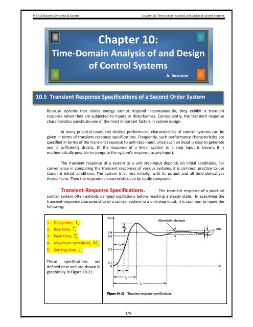
10.5 Transient Response Specifications of a Second Order System
Because systems that stores energy cannot respond instantaneously, they exhibit a transient
response when they are subjected to inputs or disturbances. Consequently, the transient response
characteristics constitute one of the most important factors in system design.
In many practical cases, the desired performance characteristics of control systems can be
given in terms of transient‐response specifications. Frequently, such performance characteristics are
specified in terms of the transient response to unit‐step input, since such an input is easy to generate
and is sufficiently drastic. (If the response of a linear system to a step input is known, it is
mathematically possible to compute the system’s response to any input).
The transient response of a system to a unit step‐input depends on initial conditions. For
convenience in comparing the transient responses of various systems, it is common practice to use
standard initial conditions: The system is at rest initially, with its output and all time derivatives
thereof zero. Then the response characteristics can be easily compared.
Transient‐Response Specifications.
The transient response of a practical
control system often exhibits damped oscillations before reaching a steady state. In specifying the
transient‐response characteristics of a control system to a unit‐step input, it is common to name the
following:
1. Delay time, T
d
2. Rise time, T
r
3. Peak time, T
p
4. Maximum overshoot, M
p
5. Settling time, T
s
These specifications are
defined next and are shown in
graphically in Figure 10‐21.
1/9

ME 413 Systems Dynamics & Control
Chapter 10: Time‐Domain Analysis and Design of Control Systems
Delay Time. The delay time T
d
is the time needed for the response to reach half of its
final value the very first time.
Rise Time. The rise time T
r
is the time required for the response to rise from 10% to
90%, 5% to 95%, or 0% to 100% of its final value. For underdamped second order systems, the 0% to
100% rise time is normally used. For overdamped systems, the 10% to 90% rise time is common.
Peak Time. The peak time T
p
is the time required for the response to reach the first peak
of the overshoot.
Maximum (percent Overshoot). The maximum percent overshoot M
p
is the
c ∞ . If
maximum peak value of the response curve [the curve of c( t ) versus t ], measured from ( )
c ( ∞ ) = 1, the maximum percent overshoot is M × 100% . If the final steady state value ( )
p
c ∞ of
the response differs from unity, then it is common practice to use the following definition of the
maximum percent overshoot:
( p ) −C( ∞)
C t
Maximum percent overshoot = × 100%
C
Settling Time. The settling time T
s
is the time required for the response curve to reach and
stay within 2% of the final value. In some cases, 5% instead of 2%, is used as the percentage of the
final value. The settling time is the largest time constant of the system.
Comments. If we specify the values of
curve is virtually fixed as shown in Figure 10.22.
T
d
,
T
r
,
T
p
,
( ∞)
T
s
and
M
p
, the shape of the response
Figure 10‐22
Specifications of transient‐response curve.
A Few Comments on Transient Response‐Specifications.
In addition of requiring a dynamic system to be stable, i.e., its response does not increase unbounded
with time (a condition that is satisfied for a second order system provided that ζ ≥ 0 , we also
require the response:
• to be fast
• does not excessively overshoot the desired value (i.e., relatively stable) and
• to reach and remain close to the desired reference value in the minimum time possible.
2/9

ME 413 Systems Dynamics & Control
Chapter 10: Time‐Domain Analysis and Design of Control Systems
Second‐Order Systems and Transient‐Response‐Specifications.
The response for a unit step input of an underdamped second order system ( 0 ζ 1)
or
ζ −ζω
t
−ζω
t
n
n
c()
t = 1− e sinω
t −e cosω
t
d
d
2
1 − ζ
⎧
−ζω
⎪ ζ
⎫
t
⎪
n
= 1− e ⎨ sinω
t + cosω
t
d
d ⎬
2
⎩⎪
1 − ζ
⎭⎪
e
< < is given by
(10‐13)
−ζω
2
1
()
t n
−
c t = 1 − sin ⎨ω
t + tan
d
⎬
(10‐14)
2
1 − ζ
⎧⎪
⎩⎪
1 − ζ ⎫⎪
ζ ⎭⎪
A family of curves c( t ) plotted against t with various values of ζ is shown in Figure 10‐24.
1.6
1.4
ζ = 0.2
Step Response
1.2
0.5
ut ( )
1
0.7
1
1
−−−−− 142 43
Input
t
s
ω
2
n
2 2
+ 2ζ ωns+
ωn
Amplitude
0.8
0.6
0.4
2
5
0.2
0
0 2 4 6 8 10 12 14 16 18 20
Output
Time (sec)
144424443
_______________
Figure 10‐24
Unit step response curves for a second order system.
Delay Time. We define the delay time by the following approximate formula:
Rise Time. We find the rise time
r
T
d
1+
07 . ζ
=
ω
n
T by letting cT ( ) 1
r
= in Equation (10‐13), or
⎧
−ζω
⎪ ζ
⎫⎪
n r
c( T)
= 1= 1− T
r
e ⎨ sinωT + cosω
d r
T
d r⎬
(10‐15)
2
⎩⎪
1 − ζ
⎭⎪
−ζωn Since e
t
≠ 0, Equation (10‐15) yields
3/9

ME 413 Systems Dynamics & Control
Chapter 10: Time‐Domain Analysis and Design of Control Systems
or
Thus, the rise
T
r
is
ζ
2
1 − ζ
sinωT + cosωT
= 0
tanω
T
d
r
d
r
d
2
1 − ζ
=−
ζ
r
r
⎛
2
−1 1 − ⎞ π −
1 ζ β
= tan −
=
ω ⎜ ζ ⎟ ω
d
⎝ ⎠
d
T (10‐16)
where β is defined in Figure 10‐25. Clearly to obtain a large value of T
r
we must have a large value
of β .
jω
ωn
2
1−
ζ
−σ
ω n
β
jω d
β = cos
σ
−1
( ζ)
( ζ )
or β = sin 1−
or
β
−1 2
⎛
1−ζ
⎞
ζ ⎟
⎠
2
−1
= tan ⎜ ⎟
⎜
⎝
ζω n
Figure 10‐25
Definition of angle β
Peak Time. We obtain the peak time T
p
by differentiating c( t ) in Equation (10‐13), with
respect to time and letting this derivative equal zero. That is,
dc ( t ) ωn
−ζωn = e
t
sinω
= 0
2
dt
dt 1−
ζ
It follows that
sinω t d
= 0
or
ω t = 0, π, 2 π, 3 π,... = n d
π, n = 0,1,2.....
Since the peak time
T corresponds to the first peak overshoot ( n = 1)
, we have ω T = π
p
π π
= =
ω
2
d ω 1−
ζ
T (10‐17)
p
n
d
p
. Then
4/9

ME 413 Systems Dynamics & Control
Chapter 10: Time‐Domain Analysis and Design of Control Systems
The peak time T
p
corresponds to one half‐cycle of the frequency damped oscillations.
Maximum Overshoot M
p
The maximum overshoot M
p
occurs at the peak
T = π ω . Thus, from Equation (10‐13),
p
d
or
⎧
⎫
n ( d )
Mp
c( Tp)
1 e ζω πω ζ − ⎪
⎪
= − = − ⎨ sinπ + cos
2
{ π ⎬
⎪ 1−ζ
1442443 = −1
⎪
⎩
⎪
= 0
⎭
⎪
p
− 1 − 2
= (10‐18)
M e πζ ζ
Since c ( ∞ ) = 1, the maximum percent overshoot is
=
− 1 − 2
×
Mp% e πζ ζ 100%
The relationship between the damping ratio ζ and the maximum percent overshoot is shown in
Figure 10‐26. Notice that no overshoot for ζ ≥ 1 and overshoot becomes negligible for ζ > 07 . .
Figure 10‐26 Relationship between the maximum percent overshoot M p
% and damping ratio ζ .
Settling Time T
s
Based on 2%criterion the settling time T
s
is defined as:
−
e ζω
nTs
= 002 .
( 002 . ) 4
ln
− ζωnTs = ln ( 002 . ) ⇒ Ts
= ≈
−ζω
ζω
n
n
5/9

ME 413 Systems Dynamics & Control
Chapter 10: Time‐Domain Analysis and Design of Control Systems
T s
4
ζω
= ( 2%Criterion)
(10‐19)
n
Similarly for 5% we can get
3
T s =
ζω
( 5%Criterion)
(10‐20)
n
REVIEW AND SUMMARY
TRANSIENT RESPONSE SPECIFICATIONS OF A SECOND ORDER SYSTEM
TABLE 1.
Useful Formulas and Step Response Specifications for the Linear
Second‐Order Model m & x&+ c x&
+ k x = f (t)
where m, c, k constants
2
− c ± c − 4mk
1. Roots
s1,2
=
2m
2. Damping ratio or ζ = c / 2 mk
3. Undamped natural frequency
ω
n
=
2
4. Damped natural frequency
ω d
= ω n
1−ζ
5. Time constant τ = 2 m / c = 1/
ζω
n
if ζ ≤ 1
k
m
6. Stability Property Stable if, and only if, both roots have negative real parts, this occurs if
and only if , m, c, and k have the same sign.
7. Maximum Percent Overshoot: The maximum % overshoot M
p
is the maximum peak value of the
response curve.
M p
= 100e
2
−πζ / 1−ζ
8. Peak time: Time needed for the response to reach the first peak of the overshoot
2
T = π / ω 1−
ζ
9. Delay time: Time needed for the response to reach 50% of its final value the first time
1+
0.
7ζ
Td
≈
ω
p
n
10. Settling time: Time needed for the response curve to reach and stay within 2% of the final value
4
Ts
=
ζω
n
11. Rise time: Time needed for the response to rise from (10% to 90%) or (0% to 100%) or (5% to 95%) of
π − β
its final value Tr
= (See Figure 10‐25)
ω
d
n
6/9

ME 413 Systems Dynamics & Control
Chapter 10: Time‐Domain Analysis and Design of Control Systems
SOLVED PROBLEMS
█ Example 1
Figure 4‐20 (for Example 1)
7/9

ME 413 Systems Dynamics & Control
Chapter 10: Time‐Domain Analysis and Design of Control Systems
█ Example 2
Figure 4‐21 (for Example 2)
█
Solution
First The transfer function of the system is
8/9

ME 413 Systems Dynamics & Control
Chapter 10: Time‐Domain Analysis and Design of Control Systems
█ Example 3 (Example 10‐2in the Textbook Page 520‐521)
T
d
,
Determine the values of
subject to a unit step input
T
r
,
T
p
,
T
s
when the control system shown in Figure 10‐28 is
Rs ( )
1
s ( s + 1)
C( s)
Figure 10‐28
Control System
█
Solution
The closed‐loop transfer function of the system is
1
C( s)
s( s+
1)
1
= =
2
R( s)
1
1+
s + s+
1
s s+
1
( )
Notice that ω
n
= 1 rad/s and ζ = 05 . for this system. So
Rise Time.
T
r
π − β
=
ω
where
−1 −
β = sin ( ω ) 1 d
ωn
= sin ( 0. 866 1)
= 1.
05rad
or
−1 −1 −
β = cos ( ζω ) cos ( ) cos
1 n
ωn
= ζ = ( 05 . )
= 105 . rad
Therfore,
π −1.05
T
r
= = 2.41 s
0.866
π π
Peak Time. Tp
= = = 363 . s
ωd
0.
866
Delay Time.
1+
0.
7ζ
1+
0. 7( 0.
5)
Td
= = = 135 . s
ω 1
n
d
ωn
ω = ω − ζ = − =
d
2
1−
ζ
Maximum Overshoot : Mp
= e e e
4 4
Settling time: Ts
= = = 8s
ζω 05 . × 1
n
−σ
n
2 2
1 1 0. 5 0.
866
ω n
β
ζω n
jω
jω d
−πζ 1−ζ 2 − π× 05 . 1−05
. 2
−181
.
= = = =
σ
0. 163 16. 3%
9/9