Performance Modeling and Benchmarking of Event-Based ... - DVS
Performance Modeling and Benchmarking of Event-Based ... - DVS
Performance Modeling and Benchmarking of Event-Based ... - DVS

Create successful ePaper yourself
Turn your PDF publications into a flip-book with our unique Google optimized e-Paper software.
42 CHAPTER 4. PERFORMANCE ENGINEERING OF EVENT-BASED SYSTEMS<br />
3XEOLVKHUS N<br />
6\VWHP<br />
[ WN [ WN<br />
[ WN<br />
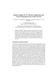
Figure 4.4: <strong>Modeling</strong> Non-Poisson <strong>Event</strong> Publications.<br />
We now show how the firing weights <strong>of</strong> the immediate transitions ϕ i for i = 1..N must be<br />
set in order to achieve the desired routing behavior. We use the notation<br />
µ : A 1 {c ′ 1 x 1 } ∧ A 2 {c ′ 2 x 2 } ∧ ... ∧ A n {c ′ n x n } → B 1 {d ′ 1 y 1 } ∧ B 2 {d ′ 2 y 2 } ∧ ... ∧ B m {d ′ m y m }<br />
to denote a transition mode µ in which c i × x i tokens are taken from place A i for i = 1..n<br />
<strong>and</strong> d j × y j tokens are deposited in place B j for j = 1..m. If an event modeled by token<br />
color x t,k visits the system node corresponding to place π i , from there it can possibly be forwarded<br />
to every node n j such that ν t,k<br />
i,j > 0. Assuming that there are m such nodes, let us<br />
denote the set <strong>of</strong> their id’s as ζ = {j 1 , j 2 , ..., j m } = {j : ν t,k<br />
i,j > 0}. For every subset <strong>of</strong> these<br />
nodes σ = {l 1 , l 2 , ..., l r } ⊆ {j 1 , j 2 , ..., j m }, we define a firing mode µ σ i <strong>of</strong> transition ϕ i as follows:<br />
µ σ i : π i {1 ′ x t,k } → π l1 {1 ′ x t,k } ∧ π l2 {1 ′ x t,k } ∧ ... ∧ π lr {1 ′ x t,k } (4.17)<br />
which means that a x t,k token is taken from place π i <strong>and</strong> a x t,k token is deposited in each<br />
<strong>of</strong> the places π l1 , π l2 , ..., π lr , as shown in Figure 4.5. This corresponds to node n i forwarding an<br />
arriving event <strong>of</strong> type e t , published by publisher p k , to nodes n l1 , n l2 , ..., n lr . In order to achieve<br />
the desired routing behavior, the firing weight ψ(µ σ i ) <strong>of</strong> the mode is set as follows:<br />
ψ(µ σ i ) = ∏ g∈σ<br />
ν t,k<br />
i,g<br />
∏<br />
g∈ζ\σ<br />
(1 − ν t,k<br />
i,g ) (4.18)<br />
To explain this, let us consider the action <strong>of</strong> node n i forwarding an arriving event to node n lh<br />
as an “event” in terms <strong>of</strong> probability theory. For h = 1..r, we have r events <strong>and</strong> their probabilities<br />
are given by ν t,k<br />
i,l h<br />
. At the same time for each g ∈ ζ \ σ we can consider the action <strong>of</strong> node n i<br />
not forwarding an event to node n g as an event. We have m − r such events in total <strong>and</strong> their<br />
probabilities are given by (1 − ν t,k<br />
i,g ). If we assume that all these events are independent, the<br />
probability <strong>of</strong> all <strong>of</strong> them occurring at the same time would be equal to the product <strong>of</strong> their<br />
probabilities. Thus, Eq. (4.18) can be interpreted as the probability <strong>of</strong> forwarding an arriving<br />
event <strong>of</strong> type e t , published by publisher p k , to nodes n lh for h = 1..r <strong>and</strong> no other nodes. Even<br />
though in reality the independence assumption might not hold, it is easy to see that by setting<br />
the firing weights as indicated above, routing behavior with equivalent resource consumption is<br />
enforced.<br />
The model we presented is focused on capturing resource contention inside the system nodes,<br />
however, it can easily be extended to also capture contention for network resources. Network<br />
links can be modeled using queueing places that event tokens visit when they are sent from one<br />
place to another. Figure 4.6 shows an example <strong>of</strong> how networks can be modeled. Nodes n i1<br />
<strong>and</strong> n i2 (represented with places π i1 <strong>and</strong> π i2 ) communicate with nodes n j1 <strong>and</strong> n j2 over a network<br />
(e.g., a LAN) modeled using queueing place χ 1 . Node n i2 communicates with node n j3 through<br />
another network modeled using queueing place χ 2 . Depending on the size <strong>of</strong> QPN models,<br />
different methods can be used for their analysis, from product-form solution methods [22] to<br />
optimized simulation techniques [127].