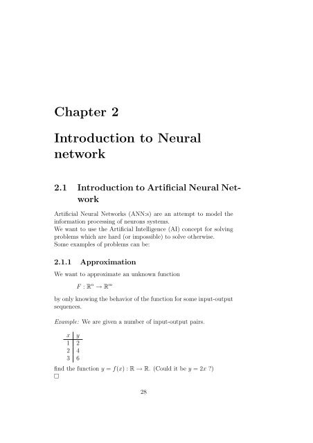
Chapter 2 Introduction to Neural network

Chapter 2
Introduction to Neural
network
2.1 Introduction to Artificial Neural Network
Artificial Neural Networks (ANN:s) are an attempt to model the
information processing of neurons systems.
We want to use the Artificial Intelligence (AI) concept for solving
problems which are hard (or impossible) to solve otherwise.
Some examples of problems can be:
2.1.1 Approximation
We want to approximate an unknown function
F : R n → R m
by only knowing the behavior of the function for some input-output
sequences.
Example: We are given a number of input-output pairs.
x y
1 2
2 4
3 6
find the function y = f(x) : R → R. (Could it be y = 2x )
□
28

Example:
¡
Many signal processing problems can be transformed to the approximation
problem. We will deal with arbitrary number of input
and output for any nonlinear function.
2.1.2 Association
The ideas is to put a finite number of items in memory (e.g. the
Latin characters) and by presenting distorted versions, we want the
item to be restored.
Example:
Input
Output
¡
□
2.1.3 Pattern classification
A number of inputs should be classified into categories.
o
¡
90 C OK
o
100 C
Error
□
2.1.4 Prediction
Given information up to present time predict the behavior in the
future.
2.1.5 Automatic control (Reglerteknik)
We want to simulate the behavior of a process so that we can control
it to fit our purposes.
29

¡¢£¤¡¢£¥ ¡ ¢£¦ § ¡¢£¤§¡¢£¥ § ¡¢£¦
¤¥¤¦ ¤ §¨¥¨¦¨§ ©
2.1.6 Beamforming
We want to create directional hearing by the use of multiple sensors.
The model
Regard the ANN as a mapping box. An input x gives an output y
The box can be feed forward (i.e. no recursions) or a recurrent
(with recursion) network. The complexity of its interior can vary
depending on the task.
The box have parameters (weights) which can be modified to suite
different tasks.
2.2 A Neuron model
Given an input signal x it create a single output value
where y = f(x T w), f : R → R, f ⊂ C 1 , any function. The vector
w = [w 1 w 2 · · · w n ] T is called the weights of the neuron. Often
w ∈ R n .
¢ ¡¢£
30

¡¢¡
¥¦¡¥¦¡¥¦¡
¡ ¤ ¢ £
£
2.3 A feedforward Network of Neurons
(3-layers)
[1]
[1]
[2] ¤ ¡¤¢¡ ¥§
[2]
[3]
[3]
[1]
¦¡¦¢¦¥
[2]
¨¢
[3]
¡¢©
Input
layer
First hidden
layer
Second hidden
layer
output
layer
[ [ [ ]] ]
⇔ y = H W [3] · G W [2] · F W [1] · x
¤ ¡¤¢¡ £¥
¤ ¡¤¢¡ §© ¨¡¨§© ¡ ¢ ¡¢£
where
F = [f 1 f 2 · · · f m ] T , G = [g 1 g 2 · · · g k ] T , H = [h 1 h 2 · · · h i ] T
and
W [1] = [w [1]
ij ] m×n, W [2] = [w [2]
ij ] k×m, W [3] = [w [3]
ij ] i×k
2.4 A recurrent Network
Z −1 -delay operator. ”The Hopfield Network”
31

2.5 Learning
Depending on the task to solve different learning paradigms (strategies)
are used.
Learning
Unsupervised
Supervised
Reinforced learning
Corrective learning
Supervised - during learning we tell the ANN what we want as
output (desired output).
corrective learning - desired signals are realvalued
reinforced learning - desired signals are true/false
Unsupervised - Only input signals are available to the ANN during
learning (e.g. signal separation)
One drawback with learning system are that it is totally lost when
facing a scenario which it has never faced during training.
32

¢¥¢¦ ¢ §¨¥¨¦¨§ ©
Chapter 3
Threshold logic
These units are neurons where the function is a shifted step function
and where the inputs are Boolean numbers (1/0). All weights are
equal to ±1
y =
{ 1 if x T w θ
0 if x T w < θ
¡¢£θ¤
¡¢£θ¤¥
θ
¢
Proposition All logical functions can be implemented with a network
of these units, since they can implement, AND, OR and NOT
function.
33

3.1 Hadamard-Walsh transform
For bipolar coding (-1/1) the Hadamard-Walsh transform converts
every Boolean function of n variables into a sum of 2 n products.
Example:
X 1 X 2 X 1 OR X 2
−1 −1 −1 f 1
−1 1 1 f 2
1 −1 1 f 3
1 1 1 f 4
The hadamard-Walsh matrix H n is defined recursively as
H n = 1 [ ]
Hn−1 H n−1
2 −H n−1 H n−1
whereby
H 1 = 1 2
[ 1 1
−1 1
]
each row/column in the matrix are orthogonal to the other rows/columns.
We want to find the coefficients a which solve the equation
by using
⎡
X 1 ORX 2 = 1 4 (a 1 + a 2 x + a 3 x 2 + a 4 x 1 x } {{ } 2 )
no. 2 2
⎢
⎣
⎡
⎢
⎣
which gives
□
a 1
a 2
.
a 2 n
⎤
⎤
a 1
a 2
a 3
a 4
⎡
⎥
⎦ = H n ⎢
⎣
⎥
⎦ = 1 4
⎡
⎢
⎣
f 1
f 2
.
f 2 n
⎤
⎥
⎦
1 1 1 1
−1 1 −1 1
−1 −1 1 1
1 −1 −1 1
⎤ ⎡
⎥ ⎢
⎦ ⎣
X 1 ORX 2 = 1 4 (2 + 2x 1 + 2x 2 − 2x 1 x 2 )
34
−1
1
1
1
⎤
⎥
⎦

¢¥¢¦ ¢ §¨¥¨¦¨§ ©
Chapter 4
The Perceptron
The perceptron is a weighted threshold logic unit.
y =
{ 1 if x T w θ
0 if x T w < θ
¡¢£θ¤
x, w ∈ R n
The perceptron can classify all input vectors belonging to linearly
separable classes.
Example:
P and N are linear separable!
□
¢£¤¥¦§ £ ¤¥¦¨ ©£ ¡
35

¢£¤¥¦§ £ ¤¥¦¨
¢¥¢¦§¡¢£¤¡¢ ¨©¢£¡£ ¡¢£ ¦£
¡¢£¢¡¡¦£
Example:
Not linear separable!
□
Example: Classification problem
©£ ¡
□
¢ ¥¢¦§
¡¢£¤¡¢
4.1 Perceptron training
¢££¦¢
Assume we have sampled the sensors when the process is OK (P)
as well as when its broken (N). We have a number of input vectors
in each class.
Start: Choose w 0 randomly, t = 0
test: Select a vector x ∈ P ∪ N
If all x correct, stop!
36

⎧
⎪⎨
⎪⎩
if x ∈ P and x T w t > 0 goto test
if x ∈ P and x T w t 0 goto add
if x ∈ N and x T w t < 0 goto test
if x ∈ N and x T w t 0 goto subtract
add: 1. w t+1 = w t + x or
w t+1 = w t − (xT w t−ε)
x , ε > 0
‖x‖ 2 2
2. t = t + 1
subtract: 1. w t+1 = w t − x or
w t+1 = w t − (xT w t +ε)
x , ε > 0
‖x‖ 2 2
2. t = t + 1
If the two sets N and P are not perfectly linear separable we want
to make a good approximation of the classification.
The pocket algorithm:
start: Initialize w 0 randomly
define the best weight vector w s = w
define h s = 0
iterate: Update w as before
Count the number h of consecutively correctly classifications.
If h > h s , set w s = w and h s = h.
Continue iterating.
37

¡ ¢£ ¤¡¤¢¤£¥¦w x
4.2 The Linear Neuron (LMS-algorithm)
Is a neuron with a linear function
Assume we have a signal x(n) which we want to transform linearly
and match a signal d(n)
¡
x
¢£ ¤¡¤¢¤£¥¦w x
TDL L
We form the error signal e(n) = d(n) − y(n). We define the instantaneous
error function
§
J = 1 2 e(n)2
We want to minimize J. we use the steepest descent approach and
calculate ∇ w J
∇ w J = ∇ w
1
2 (d(n) − wT x(n)) 2
Used the chain rule and the equation become
∇ w J = (d(n) − w T x(n)) · (−x(n)) = −e(n) · x(n)
where the −x(n) is the inner derivative. The steepest descent states
w k+1 = w k − α∇ w J
w k+1 = w k + αe(n) · x(n)
(LMS-algorithm)
38

Chapter 5
Layered Networks of
perceptrons
We have seen that a single perceptron can separate 2 linearly separable
classes. If we put several perceptrons in a multilayer network
what’s the maximum number of classification regions, i.e. what’s
the capacity of the network
Proposition Let R(m, n) denote the number of regions bounded
by m hyper-planes (of dim. n − 1) in a n-dimensional space(all
hyperplane are going through origin), then
where
Example:
R(m, n) = R(m − 1, n) + R(m − 1, n − 1)
R(1, n) = 2 , n 1
R(m, 0) = 0 , ∀m 1
(fig 6.20) R(m, n) is computed recursively.
M\N 0 1 2 3 4 5 6
1 0 2 2 2 2 2 2
2 0 2 4 4 4 4 4
3 0 2 6 8 8 8 8
4 0 2 8 14 16 16 16
5 0 2 10 22 30 32 32
6 0 2 12 32 52 62 64
39

□
A formula for R(m, n)
∑n−1
( ) m − 1
R(m, n) = 2
i
i=0
For a network with 3 hidden units with structure n−k −l −m that
is, n input nodes k first hidden nodes, l second hidden nodes and
m output nodes we get
max # regions = min{R(k, n), R(l, k), R(m, l)}
Example: Structure 3-4-2-3
Input
layer
First hidden
layer
Second hidden
layer
output
layer
The maximum of regions in 3-dimensional input space classifiable
by the network is
min{R(4, 3), R(2, 4), R(3, 2)} = min(14, 4, 6) = 4
That is the second hidden layer limits the performance ⇒ often the
hidden layers contain more units than the input and output layers.
40

¡¢£¤¥¦
¦ ¢
Chapter 6
The backpropagation
algorithm
Learning of a single neuron. Consider the following model of a neuron
¢w x+θ
¤¥¦§¤¨©¥©§©¨ ¡¢£
θ is a scalar parameter called the ”bias”. This bias gives the neuron
the possibility of shifting the function f(·) to the left or right
(positive or negative bias)
θ
Example: f(x + θ) = sign(x + θ)
¡ ¢§¤¥ ¢
¦θ=¤
We can use the same terminology as before by defining the extended
input vector ¯x = [x
θ=£¤
1 x 2 · · · x n 1] T and the extended weight
vector ¯w = [w 1 w 2 · · · w n θ] T ⇒ y = f( ¯w T ¯x)
41

Assume that we have a sequence of input vectors and a corresponding
sequence of target (desired) scalars
(¯x 1 , t 1 ), (¯x 2 , t 2 ), , · · · , (¯x N , t N )
We wish to find the weights of a neuron with a non-linear function
f(·) so that we can minimize the squared difference between the
output y n and the target t n , i.e.
min E n = min 1 2 (t n − y n ) 2 = min 1 2 e2 n
, n = 1, 2, · · · , N
We will use the steepest descent approach
¯w (n+1) = ¯w (n) − α∇ w E
We need to find ∇ w E!
1
∇ w E n = ∇ w
2 (t n − f( ¯w T ¯x } {{ n ) }
u
} {{ }
f(u)
} {{ }
h(f)
) 2
} {{ }
g(h)
The chain-rule gives ∇ w g(h(f(u))) = ∇ h g∇ f h∇ u f∇ w u
∇ h g = e n
∇ f h = t n − f(u) = −1
∇ u f = depends on the nonlinearity f(·) we choose
∇ w u = ¯x n
⇒ ¯w (n+1) = ¯w (n) + αe n ∇ u f¯x n
since f(·) is a function f : R → R, i.e. one-dimensional. We can
write ∇ u f = df
du
⇒ The neuron learning rule for general function f(·) is
¯w (n+1) = ¯w (n) + αe n
df
du¯x n
Where u = ¯w T ¯x and α is the stepsize.
OBS! If f(u) = u, that is a linear function with slope 1, the above
algorithm will become the LMS alg. for a linear neuron.
( df
du = 1 )
42

6.1 The non-linearity of the neuron
Any differentiable function f(·) can be used in the neuron. We will
use 2 different functions, bi- and unipolar sigmoid function.
6.1.1 The bipolar sigmoid function
(the tangent hyperbolic)
f(u) = tanh(γu) = 1 − e−2γu
1 + e −2γu
γ is called the slope (γ ∈ R)
Example:
tanh(γu)
1.5
1
γ = 2
γ = 1
0.5
γ = 0.25
0
0.5
1
1.5
6 4 2 0 2 4 6
u
often γ = 1.
The derivative of f(u) is
df
du = γ(1 − tanh(γu)2 ) = γ(1 − f(u) 2 )
43

6.1.2 The unipolar sigmoid function
Example:
f(u) =
1
1 + e −γu
f(u)
1.2
1
γ = 2
0.8
γ = 1
0.6
γ = 0.25
0.4
0.2
0
0.2
6 4 2 0 2 4 6
u
The derivative of f(u) is
(
)
df
du = γ 1
1
1 − = γf(u)(1 − f(u))
1 + e −γu 1 + e −γu
this gives the update formulas for the neuron
1. bipolar
¯w (n+1) = ¯w (n) − αγe n (1 − y 2 n)¯x n
y n = f(u n ) = tanh(γu n ) = tanh(γ ¯w T n ¯x n )
2. unipolar
¯w (n+1) = ¯w (n) − αγe n y n (1 − y n )¯x n
y n = f(u n ) = 1
1+e γu n
=
1
1+e γ ¯wT n ¯xn
44

6.2 The backpropagation algorithm for
a 3-layer network
[1] ©¥¡
[2]
¡[1]¢[1]¥[1]
¥£¡
¡[1]¢[1]¥[1]
¡[2]¢[2]©[2]
¡[2]¢[2]©[2]
¨©¡¡[3]¢[3]¨[3]
[3]
• ¯w [i] - is the extended weight matrix. The last column consists
of bias terms.
¤ ¡¤¢¤¥¦¢ § ¡§¢§¨ ¦¡¦©¨¡ ¢ ¡¢£
¡¢¨¡¢¨
Assume we have a set of input vectors ¯x n and a set of corresponding
target vectors t n , n = 1, 2, · · · , N (a training set)
(x 1 , t 1 ), (x 2 , t 2 ), · · · , (x N , t N )
We want to minimize the squared difference between the output y n
of the network and the target vectors t n
i.e. min
P∑
i=1
e 2 i
We first state the algorithm and then we prove it.
6.2.1 Backpropagation algorithm
Step 1. Initiate all the weight-matrices. This can be done by the
following rule. Pick values randomly in the interval (−0.5, 0.5) and
divide with fan-in, which is the number of units feeding the layer.
Example:
¯W [1] =
¯W [2] =
(rand(m, n + 1) − 0.5)
n + 1
(rand(k, m + 1) − 0.5)
m + 1
45

¯W [3] =
(rand(p, k + 1) − 0.5)
k + 1
where ”rand” is uniformly distributed in [0, 1].
Step 2. Pick a input-target pair randomly from the training set.
say (x i , t i ). Calculate the output when x i is the input according to
[
[
y i = H ¯W [3] · G[
¯W [2] · F ¯W [1]¯x ]] ]
i
where
F = [f 1 (u 1 ) [1] , f 2 (u 2 ) [1] , · · · , f m (u m ) [1] ] T
G = [g 1 (u 1 ) [2] , g 2 (u 2 ) [2] , · · · , g k (u k ) [2] ] T
H = [h 1 (u 1 ) [3] , h 2 (u 2 ) [3] , · · · , h p (u p ) [3] ] T
All functions are chosen in advance.
Step 3.
Find the weight corrections for each layer.
First define the vector e i = t i − y i .
Define the local error vector δ [s] , s = 1, 2, 3
δ [3] = diag(e) ∂H
∂u [3]
△ ¯W [3] = αδ [3] (ō [2] ) T
, α − stepsize
OBS! ō [2] is the extended vector!
( (W
δ [2] [3]
= diag
) )
T
δ
[3] ∂G
OBS! W [3] is without the biases!
△ ¯W [2] = αδ [2] (ō [1] ) T
∂u [2]
( (W
δ [1] [2]
= diag
) )
T
δ
[2] ∂F
∂u [1]
△ ¯W [1] = αδ [1]¯x T 46

(The algorithm is called backpropagation since the local error is
propagating backwards from output layer in to the hidden layers)
Step 4.Update the weight matrices.
¯W [3] = ¯W [3] + △ ¯W [3]
¯W [2] = ¯W [2] + △ ¯W [2]
¯W [1] = ¯W [1] + △ ¯W [1]
Return to step 2, stop when no changes in △ ¯w [s]
□
The partial derivative are
[
∂H
=
∂u [3]
dh 1
du [3]
1
dh 2
du [3]
2
. . .
dh m
du [3]
m
If we use the bipolar sigmoid function
∂H
∂u [3] =
and the same follows for ∂G
∂u [2]
] T
[
(1 − tanh(u [3]
1 ) 2 ) (1 − tanh(u [3]
2 ) 2 ) . . . (1 − tanh(u [3]
m ) 2 )
and ∂F
∂u [1]
6.3 The proof of the Back propagation
We first define the error function for input-target pair i ′ , i.e. (x i ′, t i ′)
E i ′ = 1 p∑
(t ji ′ − y ji ′) 2 = 1 p∑
e 2 ji
2
2
= 1 ′ 2 ‖e i ′‖2 2
j=1
that is we want to minimize the sum of the squared errors.
For every weight w [s]
ji in layer s = 1, 2, 3 we will use the steepest
descent rule to update the weight
w [s]
ji
= w [s]
ji − α ∂E i
∂w [s]
ji
j=1
= w [s]
ji + △w[s] ji
We need to find the partial derivative ∂E i ′
for every weight in every
∂w [s]
ji
layer. First we start with the outputlayer (s = 3)
− ∂E i ′
∂w [3]
ji
= − ∂E i ∂u [3]
′ j
∂u [3]
j ∂w [3]
ji
47
] T

where
u [3]
j =
p∑
i=1
w [3]
ji o[2] i
we define the local error δ [3]
j
as
δ [3]
j = − ∂E i ′
∂u [3]
j
= − ∂E i ′ ∂e ji ′
∂e ji ′
∂u [3]
j
= e ji ′
∂h j
∂u [3]
j
And we get the update rule for all weights in the output layer
(s = 3) as
w [3]
ji = w [3]
ji + αe ji ′
∂h j
∂u [3]
j
o [2]
i = w [3]
ji + αδ[3] j
Which is the same rule as for the single neuron where the input o [2]
is the output from previous layer.
We continue to derive the update for the second hidden layer (s = 2)
As before
− ∂E i ′
∂w [2]
ji
= − ∂E i ∂u [2]
′ j
∂u [2]
j ∂w [2]
ji
= δ [2]
j o[1] i
The calculation of the local error δ [2]
j
will be different
δ [2]
j = − ∂E i ′
∂u [2]
j
= − ∂E i ∂o [2]
′ j
∂o [2]
j ∂u [2]
j
o[2] i
for the second hidden layer
since o [2]
j = g j (u [2]
j ) where g j(·)- the function associated with neuron
j.
We have
δ [2]
j = − ∂E i ′ ∂g j
∂o [2]
j ∂u [2]
j
To calculate − ∂E i ′
we use the chain rule once again to express the
∂o [2]
j
derivative in terms of the local error in layer 3.
− ∂E i ′
∂o [2]
j
= −
p∑ ∂E i ′
i=1
∂u [3]
i
∂u [3]
i
∂o [2]
j
48
=
( )
p∑
− ∂E i ′
i=1
∂u [3]
i
} {{ }
=δ [3]
i
∂
∂o [2]
j
p∑ (
k=1
w [3]
ik o[3] k
)
} {{ }
u [3]
i

The sum comes from the fact that one output o j in layer 2 is connected
to all u i in layer 3.
− ∂E i ′
∂o [2]
j
=
p∑
i=1
δ [3]
i w [3]
ij
which gives the update rule for the second hidden layer
w [2]
ji = w [2]
ji + αδ[2] j
o[1] i
where
δ [2]
j
= ∂g j
∂u [2]
j
p∑
i=1
δ [3]
i w [3]
ij
In the same way the update for the first hidden layer can be derived
using the local error of the following layer
where
w [1]
ji = w [1]
δ [1]
j
= ∂f j
∂u [1]
j
ji + αδ[1] j x i
k∑
i=1
δ [2]
i w [2]
ij
Using matrix notation the algorithm is derived.□
49

6.4 The rule of the hidden layer
Consider a two layer feedforward neural network, one hidden and
one output layer, without non-linearities The output vector will
x
y
w
[1] [2]
w
then be
y = W [2] (W [1] x) ⇔ y = Wx
which means that the network con be reduced to a single layer network
with weight matrix W = W [2] W [1] .
⇒ Every multilayer feedforward network with linear neurons can
be reduced to an equivalent single layer network.
Proposition A three layer feedforward neural network with sigmoidal
functions can approximate any multivariate function, with
finite number of discontinuities, at any desired degree of accuracy.
□
Provided we have enough number of neurons.
6.5 Applications of back-propagation alg.
the solution to a set of linear equations
Ax = b
(A can be any size (m × k))
⇒ x opt = A + b
(in the LS-sense if no solution exists)
How can we use Neural networks to find the pseudo-inverse of A
We will use a single layer NN with linear neurons (no biases). Write
the matrix A as
A T = [a 1 a 2 · · · a m ]
50

x
w
y
¡¢£¤
and define the columns of a identity matrix
I m×m = [e 1 e 2 · · · e m ]
i.e.
⎡ ⎤ ⎡ ⎤ ⎡ ⎤
1 0
0
e 1 = ⎢ ⎥
⎣
0. ⎦ , e 2 = ⎢ ⎥
⎣
1. ⎦ , . . . , e m = ⎢ ⎥
⎣
0. ⎦
0 0
1
then the training set is
(a 1 , e 1 ), (a 2 , e 2 ), · · · , (a m , e m )
we use the LMS algorithm to adapt the weights W to the training
set with one modification, that is
W (k+1) = (1 − γ)W k + αex T
γ ≪ 1- leaky factor, α - stepsize, x k =input=a k and e = error vector
(remember we have linear functions, the algorithm is the MIMO-
LMS, Multiple-Input Multiple-Output)
After convergence W T = A + (Pseudoinverse of A) □
6.5.1 One more example of Backpropagation
An alternative way to find the pseudo inverse of a matrix A.
We will use a linear two layer network. We create a random sequence
of input vectors and use the same vectors as targets.
⇒ Training sequence(x 1 , x 1 ), (x 2 , x 2 ), . . . , (x N , x N )
We fix the first layer weights to A and we only update the output
layer weights W.
51

¤
A
¤
W
¢£
Since we know that for any input vector x
¡ ¡
i
¢£
we have
ˆx i = WAx i
and that backpropagation minimizes the norm of
min ‖ x i − WAx i ‖ ⇒ W = A +
6.6 Application speech synthesis-NETtalk
People in the field of linguistics have been working with rule based
speech synthesis systems for many years.
Speech synthesis is away of converting text to speech and a feedforward
neural network, NETtalk, can be trained to solve this.
Is uses a 7 character sliding window to read the text and it is trained
with backpropagation to classify the phonemes of the text’s pronunciation
(See figure 9.14).
Phonemes
26 output units
80 hidden units
u r a l _ N e
7 groups of
29 input sites
Another application is the reverse problem of listening to speech
and then convert to text. They use Hidden Markov Models trained
with Backpropagation.
6.7 Improvements to backpropagation
There are many ways to improve the convergence of backpropagation.
52

Main problem is the steepest descent algorithm. We know that
steepest descent is perpendicular to the contours of the error function.
closest path
We also know that the more elliptic the contour is the slower the
convergence will be. The ratio of the ellipses diameters are controlled
by the eigenvalues of the correlation matrix R xx (x-input).
If we decorrelate the input before the network we will get better
performance.
λ
2 λ
1
λ− eigenvalues of R xx
Decorrelation can be done by an unsupervised algorithm (The Generalized
Hebbian algorithm) by finding the Principal Components
(PCA). We will se this later in this course.
6.8 Momentum update
In order to drop faster in the error surface we use the average of
previous gradients when we update the weights
△w (k)
ij
= − ∂E + β△w (k−1)
ij
∂w ij } {{ }
momentum term, β

The backpropagation algorithm can cause the weight update to follow
a fractal pattern (fractal means it follow some rules which are
applied statistical), (see figure 8.11)
⇒ The stepsize and momentum term should decrease during training
to avoid this.
6.9 Adaptive step algorithms
These algorithms modifies the stepsize during training in order to
speed convergence. The idea is to increase the stepsize,α , if the
sign of the gradient is the same for two following updates and to
decrease if the sign change.
Example: Error function
start
increase
decrease
increase
6.10 Silva and Almeidal’s algorithms
α (k+1)
i =
{
α (k)
α (k)
i u if ∇ i E (k) ∇ i E (k−1) > 0
i d if ∇ i E (k) ∇ i E (k−1) < 0
u, d parameters (e.g. u = 1.1, d = 0.9) and index i stands for weight
no. i
□
Other similar methods are Delta-bar-delta and and Rprop.
6.11 Second order algorithms
These methods use the Newton’s algorithm instead of the steepest
descent.
[ ] ∂
w (k+1) = w (k) 2 −1
E
− ∇
∂w 2 w E
54

One can derive the updates for the network in each layer as before
but the computational complexity will increase drastically in the
training of the network.
Every neuron needs a matrix inversion!
There are good approximations to these algorithms, the so called
Pseudo-Newton’s methods, e.g. Quickprop, QRprop etc.
6.12 Relaxation methods
These methods are used to avoid calculating the gradient. They
use a trial and error approach, change the weights in any way
- if the error is dropping use the new weights otherwise try again.
6.13 Generalization
The learning process may be viewed as a ”curve-fitting” problem.
The network itself may be considered simply as a non linear inputoutput
mapping.
When training Neural Networks it is important to get a network
that has good generalization. A network is said to ”generalize” well
when the input-output mapping computed by the network is correct
(or nearly so) for test data never used in creating or training the
network.
Over-fitting is one of the biggest threats to a good generalization.
Over-fitting occurs during training when the number of free
parameters, or weights, is too large. What happens is that the error
during training is driven to a very small value, but when new
data is presented to the network the error is large. This depend on
that the networks complexity is too big which results in that the
entire training patterns is memorized and that it has big enough
degree of freedom to fit the noise perfectly. Of course this means
bad generalization to new test data. The figure tries to visualize
this problem. One solution to this problem is to reduce the number
of free parameters. This is easiest done by reducing the number of
hidden neurons. Generalization is influenced by three factors:
• The size of the training set, and how representing it is for the
environment of interest.
55

x - training data
o - generalization
- non linear mapping
x
x
o
x
x x x
x
x
o
x
x x x
x
x
Good fit but bad generalization
Bad fit but much better generalization
• The architecture of the neural network
• The physical complexity of the problem of hand.
We may view the issue of generalization from two different perspectives.
• The architecture of the network is fixed. We have to determine
the size of the training set needed for a good generalization
to occur.
• The size of the training set is fixed. We have to determine
the best architecture of the network for achieving good generalization.
6.13.1 The size of the training set
We May in generally say that for good generalization, the number
of training examples P should be larger than the ratio of the total
number of free parameters (the number of weights) in the network
to the mean square value of the estimation error.
6.13.2 Number of hidden neurons
To choose the correct number of hidden neurons is an important
aspect when designing a Neural Network. Too few hidden neurons
gives us a net that has difficulty to adapt to the training data and
too many neurons may result in a network with bad regularization.
A theoretical and a more straightforward approach on finding the
number of neurons will be discussed in the following subsections.
56

A theoretical approach
How many neurons should be used in relation to the number of
training examples Information theory suggests that the number
of input vectors should be equal to the number of weights in the
system. The number of weights, W, for a multi-layer network can
be calculated by the expression:
W = (I + 1)J + (J + 1)K (6.1)
where I is the number of inputs, J the number of hidden neurons
and K is the number of outputs. Another point of view is the
one from Widrow and Lehr (1990). They argue that the number
of training examples P should be much greater than the network
capacity, which is defined as the number of weights divided by the
number of outputs (W/K). In their paper they also refer to Baum
and Hesslers (1989) statement that the number of training examples
into a multi-layer network could be calculated as follows:
P = W (6.2)
ε
where ε is an ”accuracy parameter”. An ”accuracy parameter”
means the fraction of tests from the test set that are incorrectly
classified. A good value for ε is 0, 1, which corresponds to an accuracy
level of 90%. This gives us the rule of thumb below.
Lower bound for number of input examples, P , is P = W . And
a realistic upper bound for P is P = 10W .
This is just a rule of thumb and there is actually no upper bound
for P .
Example
Suppose we know the number of training examples P and we
would like to calculate the number of hidden neurons. The inputvector
is of length 24, I = 24, and the number of training examples
is 4760, P = 4760. The number of outputs is one, K = 1. This
gives us the following equations:
W = (24 + 1)J + (J + 1)1 ⇔ W = 26J + 1 (6.3)
Since the rule of thumb says that,
W ≤ P ≤ 10W ⇔ (26J + 1) ≤ 4760 ≤ (260J + 10) (6.4)
we get that the limitations for the hidden neurons, J.
18 ≤ J ≤ 183 (6.5)
57

6.13.3 Cross validation
A standard tool in statistics known as cross-validation provides an
appealing guiding principle. First the avalible data set is randomly
partitioned into a training set and a test set. The training set is
further partitioned into two disjoint subsets:
• Estimation subset, used to select the model.
• Validation subset, used to test or validate the model.
The motivation here is to validate the model on a data set different
from the one used for parameter estimation. In this way we
may use the training set to assess the performance of various candidate
models, and thereby choose the ”best” one. There is, however,
a distinct possibility that the model with the best-performing parameter
values so selected may end up overfitting the validation
subset. To guard against this possibility, the generalization performance
of the selected model is measured on the test set, which is
different from the validation subset.
Extremely low training error is not hard to achieve when training
Neural Networks. But a low training error does not automatically
mean that the training result is good. Two methods that
can improve generalization, regularization and early stopping, are
shortly discussed in the following subsections.
Early Stopping
The training set is used to calculate the gradients and to update
the network weights and biases. And as the number of epochs
increase the mean square error usually decrees. It is possible for
the network to end up over-fitting the training data if the training
session is not stopped at the right point. The validation set
is used to improve generalization. During training the validation
error is monitored. As long as the network shows no signs of overfitting,
the validation error is normally decreasing. The sign that
the method is waiting for is when the error goes from decreasing
to increasing, which means that the network starts to over-fit. The
training is stopped when the error has been increased for a specific
number of steps and the weights and biases at the minimum validation
error are returned.
58

Mean-
squared
error
Validation
sample
Early
stopping
point
Training
sample
Number of epochs
Regularization
There are a couple of regularization techniques to be used which
all are based on the same idea, to generate a smooth mapping that
does not fit the noise in the training data. This means that overfitting
should not be a problem, even when the network has lots of
hidden neurons.
The basic idea of regularization is that the squared error function,
or performance function, E mse is added with a penalty function
Ψ, to get a new error function E msereg . Here we define the
penalty function as the square norm of the weight vector in the
network, but there are other definition as well. The error function
is usually given by:
E mse = 1 N
N∑
(e i ) 2 (6.6)
i=1
where e i is network error and N the number of errors. The penalty
function:
Ψ = 1 n∑
(w j ) 2 (6.7)
n
j=1
where w are the weights and j the number of weights. These two
functions, together with a multiplicative constant µ can be used to
get a regularized error function:
E msereg = µE mse + (1 − µ)Ψ (6.8)
Using this error function, weights and biases will be forced to
small values which smoothes the network response and makes it
less likely to over-fit. To use a regularization method is especially
important when the amount of training data is limited.
59