Conics, Quadrics, and Projective Space - STEM2
Conics, Quadrics, and Projective Space - STEM2
Conics, Quadrics, and Projective Space - STEM2

You also want an ePaper? Increase the reach of your titles
YUMPU automatically turns print PDFs into web optimized ePapers that Google loves.
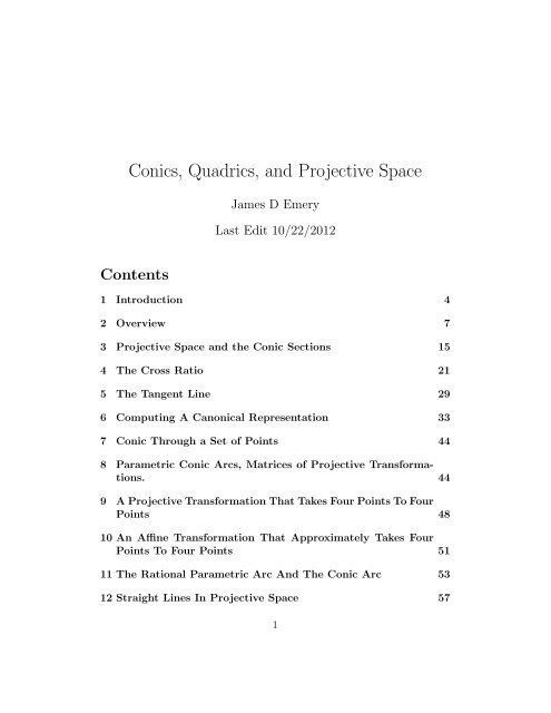
<strong>Conics</strong>, <strong>Quadrics</strong>, <strong>and</strong> <strong>Projective</strong> <strong>Space</strong><br />
James D Emery<br />
Last Edit 10/22/2012<br />
Contents<br />
1 Introduction 4<br />
2 Overview 7<br />
3 <strong>Projective</strong> <strong>Space</strong> <strong>and</strong> the Conic Sections 15<br />
4 The Cross Ratio 21<br />
5 The Tangent Line 29<br />
6 Computing A Canonical Representation 33<br />
7 Conic Through a Set of Points 44<br />
8 Parametric Conic Arcs, Matrices of <strong>Projective</strong> Transformations.<br />
44<br />
9 A <strong>Projective</strong> Transformation That Takes Four Points To Four<br />
Points 48<br />
10 An Affine Transformation That Approximately Takes Four<br />
Points To Four Points 51<br />
11 The Rational Parametric Arc And The Conic Arc 53<br />
12 Straight Lines In <strong>Projective</strong> <strong>Space</strong> 57<br />
1
13 Quadric Surfaces 59<br />
14 Quadric Surfaces And Their Matrices 60<br />
15 Transformations 63<br />
16 The Construction Of Solids 67<br />
17 Plane Image 68<br />
18 Monte Carlo Integration 68<br />
19 Stratified sampling 72<br />
20 Point Transformations <strong>and</strong> Coordinate Transformations 74<br />
21 Cross Product, Axial Vectors 75<br />
22 Angular Velocity 77<br />
23 Angular Momentum And The Inertia Tensor 79<br />
24 Surface Integrals 81<br />
25 Volume Integral 83<br />
26 Polygon Areas 84<br />
27 Perspective Projection 85<br />
28 The Tektronix Hardware Modeler: A Quadric Solid Modeler<br />
92<br />
29 References <strong>and</strong> bibliography 94<br />
2
List of Figures<br />
1 Points of projective 2-space are lines in 3-space. A 3-d linear<br />
transformation is a 2-d projective transformation. A rotation<br />
of the cone can project the circle to an ellipse, a parabola, or<br />
ahyperbola. Inthesamewaythe lines through any figure in<br />
the plane are a projective space representation of the figure.<br />
Any sequence of perspective projections of a figure onto a set<br />
of planes can be represented as a sequence of linear transformations<br />
in 3-space. The plane shown in the figure is known<br />
as the affine plane. . . . . . . . . . . . . . . . . . . . . . . . . 9<br />
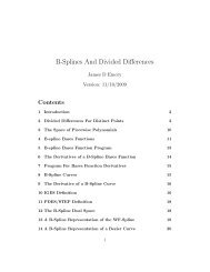
2 Let lines PQ<strong>and</strong> PRbe tangent to the ellipse. Tangent points<br />
Q <strong>and</strong> R are on the polar of P . Thus the line defined by Q<br />
<strong>and</strong> R is the polar of P . Intersection point S is on both the<br />
polar of P <strong>and</strong> the polar of P ′ .ThusthepolarofS is the line<br />
through P <strong>and</strong> P ′ . . . . . . . . . . . . . . . . . . . . . . . . . 25<br />
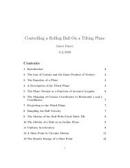
3 The parabola x − 2yz = 0 <strong>and</strong> a point at infinity Q. The line<br />
through P <strong>and</strong> Q meets the parabola at P <strong>and</strong> Q. Thepolar<br />
of a point at infinity is a diameter. The polar of Q is the line<br />
at infinity. . . . . . . . . . . . . . . . . . . . . . . . . . . . . 28<br />
4 The parabola x − 2yz = 0 <strong>and</strong> a point at infinity Q =(1, 1, 0).<br />
The line through P <strong>and</strong> Q meets the parabola at two finite<br />
points. The polar of Q is the line x = 1, which is a diameter<br />
of the parabola. The point at in finity in the diagram is<br />
represented as an arrow in the direction of the infinity point Q. 30<br />
5 Results of plotting conics with the program pltconic.ftn.<br />
(a)Ellipse with equation 10x 2 +10xy+20y 2 +3x+−4y−10 = 0,<br />
(b)Hyperbola with equation 5x 2 +10xy −7y 2 −3x+2y −1 =0,<br />
(c)Parabola with equation x 2 +6xy +9y 2 +3x − 5y − 1=0,<br />
(d)<strong>and</strong> a circle with equation 2x 2 +2y 2 + 1x − 1 y − 1=0. . 45<br />
2 5<br />
6 A conic passing through four points defined by the products of<br />
lines passing through the points (1, 1), (2, 2), (2, 1), (3, 3). The<br />
general equation of such a conic is λ(y − x)(y − x +1)+(1−<br />
λ)(y − 2)(y − 1) = 0 where λ is a parameter. Here λ =1/2.<br />
By letting points come together we can also define conics by<br />
tangent lines. . . . . . . . . . . . . . . . . . . . . . . . . . . . 46<br />
3
7 (a)Any conic arc can be obtained by mapping this parabola,<br />
which is defined by tangent lines AC <strong>and</strong> BC, <strong>and</strong> point<br />
D,where A =(0, 0),B =(1, 1),C =(0, 1/2),D =(1/4, 1/2).<br />
(b)An example of mapping the parabola to a conic representation<br />
of a circle. The intersection of the tangents is at C,<br />
which is a point at infinity. . . . . . . . . . . . . . . . . . . . 47<br />
8 A Perspective drawing showing, a building, a railroad track,<br />
<strong>and</strong> the horizon. The vanishing point at the end of the railroad<br />
tracks is at infinity in three space, yet its projection is a finite<br />
point on the two dimensional page. The figure was generated<br />
with program tracks.ftn. . . . . . . . . . . . . . . . . . . . . 86<br />
9 The intersection of the parabolic cylinder z 2 = y <strong>and</strong> the cone<br />
y 2 = xz is the union of the twisted cubic curve <strong>and</strong> the line<br />
along the x axis. This figure was generated with the solid<br />
modeling program Quadric. . . . . . . . . . . . . . . . . . . . 93<br />
1 Introduction<br />
Quadric solids are solids bounded by quadric surfaces. Quadric solids provide<br />
a rich collection of sets for constructing models of 3-dimensional objects.<br />
A large set of quadric solids may be built by combining primitive quadric<br />
solids, such as spheres, ellipsoids, blocks, cones, wedges, <strong>and</strong> cylinders. Many<br />
manufactured objects are combinations of quadric shapes. There are 17 types<br />
of quadric surfaces, including such less common surfaces as the parabolic<br />
hyperboloid.<br />
The world is full of objects built from rectangular blocks, circular cylinders,<br />
<strong>and</strong> spheres. These objects are quadric solids. Polyhedra are quite<br />
common in nature. Minerals <strong>and</strong> crystals often take a polyhedral form. Some<br />
viruses have the shape of a polyhedron. Polyhedra are quadric solids becuase<br />
they can be built from planar half spaces, <strong>and</strong> planes are quadric surfaces<br />
(pairs of planes). Essentially all objects can be approximated, to an arbitrary<br />
accuracy with polyhedra. More specifically, their surfaces may be<br />
approximated with triangles.<br />
But a polyhedron is locally flat <strong>and</strong> has no local curvature. So the planar<br />
faces of a polyhedron can not model a local curved shape exactly. An advantage<br />
of using quadric surfaces is that they can locally approximate curvature<br />
4
<strong>and</strong> shape [O’Neil p.202]. An object can be represented by a relatively small<br />
number of primitive quadric solids. If we regard atoms as tiny balls, then in a<br />
sense, all objects are built from spheres. But Avogadro’s number 6.03 × 10 23<br />
is very large, so modeling with spheres is somewhat impractical. However, in<br />
the field of scientific visualization we do model with rectangular cells defined<br />
by very large numbers of lattice points. When modeling simple manufactured<br />
parts, we are interested in finding exact models. Quadric solids can<br />
serve well in such modeling.<br />
Quadric solids by themselves do not give a full practical set of primitives<br />
for modeling. For example, surfaces of revolution are ubiquitous. But most<br />
surfaces of revolution are not quadric surfaces. Further a large number of<br />
quadrics are frequently required to get an acceptable approximation to a<br />
surface of revolution. The torus is a surface of revolution that is not a<br />
quadric surface. A torus could be approximated by a set of cylinders. But<br />
the differential geometric properties would not be approximated. Parametric<br />
free form surfaces, such as spline surfaces, are widely used in manufacturing,<br />
but are not quadric surfaces.<br />
Computations with quadric solids are simple. The calculation of a normal<br />
direction, at a point on a quadric surface, is accomplished by a matrix multiplication.<br />
The intersection points of a straight line with a primitive quadric<br />
solid require only the solution of a quadratic equation. The transformed<br />
equation of a translated or rotated quadric surface is easily found.<br />
With the advent of the computer age, there has been a renaissance of<br />
calculation. Many well known algorithms <strong>and</strong> calculating methods, while<br />
theoretically powerful, were formerly of little interest. They were two burdensome<br />
for the human computer. In the past techniques were emphasized<br />
that could be carried out easily by h<strong>and</strong>. But now those calculations, which<br />
were too lengthy for h<strong>and</strong> calculation, are proper for computer modeling <strong>and</strong><br />
computer graphics. Frequently the novice in geometric modeling <strong>and</strong> graphics<br />
does not use the proper tools. Naturally he uses the calculations taught<br />
him in the schools <strong>and</strong> colleges, which are often only the small amount of analytic<br />
geometry found in the calculus course, <strong>and</strong> deals, for example, with the<br />
simultaneous solution of a system of equations in a fixed coordinate system.<br />
A vector approach is superior for many calculations. The vector methods<br />
tend to be independent of the coordinate system. Those with scientific education<br />
are usually familiar with vectors. But they are frequently unaware of<br />
some very useful mathematics. This is the mathematics of projective geom-<br />
5
etry, projective space, <strong>and</strong> specifically the idea of homogeneous coordinates.<br />
<strong>Projective</strong> space is very important in certain advanced areas of mathematics.<br />
It is an important aspect of the field of algebraic geometry. But even<br />
among mathematicians, knowledge of projective <strong>and</strong> algebraic geometry is<br />
not universal.<br />
Often the course in projective geometry, which is offered in American<br />
universities <strong>and</strong> colleges, is designed for future teachers of high school mathematics.<br />
This course, or a course called modern geometry, is taught to show<br />
the future teacher of Euclidean geometry, that there are many geometries,<br />
<strong>and</strong> that not all of the geometries are Euclidean. Niether the course on<br />
projective geometry, nor the books designed for it, emphasize the beautiful<br />
simplifications <strong>and</strong> generalizations of calculation that come from treating<br />
points as belonging to projective space. The few pages discussing projective<br />
space in Birkhoff <strong>and</strong> MacLane (Survey of Modern Algebra), are more<br />
illuminating than the numerous pages of the elementary books on projective<br />
geometry. This is because the connection to linear algebra <strong>and</strong> vector spaces<br />
is not exploited in these books.<br />
The purpose of this report is, first to describe a modeling system which<br />
uses quadric solids as primitive objects, <strong>and</strong> second to present some elementary<br />
ideas of projective geometry which are useful for computing. These<br />
latter ideas, although elementary, are not readily available. The quadric solid<br />
modeling system is implemented in a computer program. An original version<br />
was called Quadric. A later version is called QS90.FTN. It produces<br />
views of 3-dimensional objects, calculates volumes, calculates moments, <strong>and</strong><br />
calculates inertia tensors.<br />
The idea of representing objects as primitive solids was quite fashionable<br />
in the 1980’s. Now most solid modeling systems are surface modeling systems.<br />
But primitive solid modeling still has some interest. Quadric solids<br />
are obvious c<strong>and</strong>idates for the primitives. There are several papers dealing<br />
with quadric surfaces [Leven].<br />
The modeling system described here represents objects as Boolean combinations<br />
of quadric half space primitives. An image of the model is made<br />
by scanning its surface <strong>and</strong> calculating an illumination intensity at each surface<br />
point. The 2-dimensional picture plane is scanned to construct intensity<br />
values. A surface normal is calculated at the point on the surface, where<br />
the line through the picture point pierces the object. The intensity value is<br />
determined from the inner product of the normal at the first pierce point<br />
6
with an illumination vector. Since the primitives are quadric solids, this can<br />
be done easily.<br />
A quadric surface is the set of real zeros of a quadratic form in four<br />
dimensions. Such a set of zeros is called a variety in algebraic geometry. A<br />
quadratic form is a polynomial in which each term is of the second degree.<br />
The set of points were the form takes nonpositive values is call a lower half<br />
space. An upper half space is the set where the form takes nonnegative<br />
values. A quadric form defines two quadric half spaces. Examples of half<br />
spaces are the points inside an ellipsoid, <strong>and</strong> the points outside two parallel<br />
planes.<br />
It is easy to find the intersection points of a quadric surface with a straight<br />
line. The parameters of the intersection points on the line will be the roots<br />
of a quadratic equation. Surface normals are also easily calculated.<br />
The objects are built using the st<strong>and</strong>ard set operators, union, intersection<br />
<strong>and</strong> complementation. Some modeling schemes, for example the PADL<br />
system, which was developed at the university of Rochester, uses regularized<br />
set operators. These operators guarantee that the resulting objects are<br />
topologically closed, <strong>and</strong> homogeneously three dimensional. Using st<strong>and</strong>ard<br />
operators one may get a set that is not closed. Because we have only an approximate<br />
model of the surface <strong>and</strong> do not explicitely calculate the boundary,<br />
the use of regularized operations does not seem appropriate. For intersection<br />
points which are c<strong>and</strong>idates to be on the boundary, We construct a small<br />
line segment in the direction of the normal that contains the point. If one<br />
end of the segment is inside, <strong>and</strong> the other outside, the point is a boundary<br />
point of the object.<br />
2 Overview<br />
We shall start with two-dimensional projective space. This space is easy to<br />
visualize. <strong>Projective</strong> 2-space is the set of lines in 3-dimensional space which<br />
pass through the origin. <strong>Projective</strong> 2-space is the set of one dimensional subspaces<br />
of a 3-dimensional vector space. A plane that does not pass through<br />
the origin is given a special role. It is called the affine plane. A coordinate<br />
system is usually selected so that the affine plane is the plane z =1. The<br />
idea of projective space can be illustrated by considering the intersection of<br />
a cone <strong>and</strong> a plane. The intersection curve is called a conic section. See Fig.<br />
7
1.<br />
When the cone is rotated, the conic section is transformed to a new conic<br />
section. A circle may go into a hyperbola, a parabola, or an ellipse. The<br />
lines on the cone are points of projective 2-space. The intersection of these<br />
lines with the affine plane are the representation of the points in affine space.<br />
However the projective points (i.e. lines) <strong>and</strong> the affine points are to be<br />
considered the same objects, namely 2-dimensional points. The components<br />
of any vector which lies in the subspace representing a projective point, are<br />
called the homogeneous coordinates of the point. Homogeneous coordinates<br />
are determined only up to a scalar multiple. A line in 3-space which is parallel<br />
to the affine plane meets it at infinity. The projective point in the direction<br />
of this line is called a point at infinity. Tts z coordinate will be zero. The<br />
property of being a point at infinity depends on the particular affine plane<br />
selected.<br />
In Fig. 1, if after the cone is rotated to produce an ellipse in the plane,<br />
we fix the plane to the rotated cone <strong>and</strong> then rotate the cone back to its<br />
original position, then we see that we have a perspective projection from the<br />
circle on one plane to an ellipse on a second plane. And we see that such a<br />
perspective projection is essentially the same as the 3d linear transformation,<br />
namely the original rotation of the cone. Again suppose a figure in the<br />
plane is translated in the plane with the lines joining the points of the figure<br />
following the translation. This is clearly a linear transformation of the lines<br />
or more precisely of the vectors in the direction of the lines. The plane figure<br />
would be translated the same if we were to translate the origin or cone vertex<br />
with the translation of the plane figure. So we see that the shifting of the<br />
point of perspective projection is equivalent to a linear transformation of<br />
the 3-d space. So suppose we project a figure from one plane to a second,<br />
<strong>and</strong> then from the second figure to a third figure on a third plane from a<br />
second perspective point. Then we see from what we have said before that<br />
this is equivalent to a set of linear transformations of the fixed 3-d space,<br />
namely rotations, translations <strong>and</strong> possibly a uniform scaling. So the study<br />
of these sequences of perspective projections, which were the original subject<br />
of projective geometry may be studied by considering linear transformations<br />
of one dimensional subspaces of a 3 dimensional vector space, or of a n<br />
dimension vector space in general. One can illustrate this equivalence easily<br />
in the one dimensional case by drawing sequences of perspective projections<br />
of points on lines, <strong>and</strong> then showing how the planes can be lined up parallel<br />
8
Figure 1: Points of projective 2-space are lines in 3-space. A 3-d linear<br />
transformation is a 2-d projective transformation. A rotation of the cone can<br />
project the circle to an ellipse, a parabola, or a hyperbola. In the same way<br />
the lines through any figure in the plane are a projective space representation<br />
of the figure. Any sequence of perspective projections of a figure onto a set of<br />
planes can be represented as a sequence of linear transformations in 3-space.<br />
The plane shown in the figure is known as the affine plane.<br />
9
y rotations <strong>and</strong> translations so that there is a single perspective projection<br />
point, projecting points onto a stack of parallel planes, which by scaling can<br />
be made to coincide.<br />
Now consider a 2-dimensional line. We may view it as a line lying in the<br />
affine plane. The points of this line in projective space, will be the locus of<br />
lines which pass through it <strong>and</strong> the origin. It is a plane in 3-space. Because<br />
any two planes with a point in common must coincide or meet in a line, it<br />
follows that any 2-dimensional lines in projctive space meet in a point. Two<br />
parallel lines meet at a point at infinity. Notice that 2-dimensional projective<br />
space contains more points than affine space, that is it contains the points<br />
at infinity. In two dimensional space an affine transformation is the sum<br />
of a linear transformation <strong>and</strong> a translation. If the linear transformation is<br />
orthogonal (i.e. a rotation) then the affine transformation is a rigid motion<br />
or a congruence. Now any nonsingular linear transformation maps the set of<br />
one dimensional subspaces onto itself. So we may consider such a mapping as<br />
taking 2-dimensional projective points to projective points. Such a mapping<br />
is thus called a projective transformation. These transformations distinguish<br />
euclidean, affine, <strong>and</strong> projective geometry . This is the thesis of Felix Klein.<br />
This is the essence of his famous Erlangen program. He defined a geometry<br />
to be the study of the invariants of a group of transformations. Thus the<br />
concept of angle is a property of euclidean space because angle is invariant<br />
under a rigid motion. Parallelism belongs to affine geometry because it is<br />
preserved under an affine transformation. Being a conic section is a property<br />
of projective geometry, because it is preserved under a projective transformation.<br />
Being an ellipse, however, is not a projective property. There is a<br />
projective transformation that takes an ellipse to a different type of conic<br />
section.<br />
We shall now discuss one of the major reasons for using homogeneous<br />
coordinates for calculations. An affine transformation is a special case of a<br />
projective transformation. Since a projective transformation is in essence a<br />
linear transformation in a higher dimensional space, it can be represented<br />
by a matrix, <strong>and</strong> the transformation of a point may be accomplished with<br />
matrix multiplication. An affine transformation is represented as a matrix<br />
multiplication. There many advantages to using homogeneous coordinates.<br />
<strong>Quadrics</strong> are represented homogeneously as quadratic forms, <strong>and</strong> can be<br />
represented as symmetric matrices. Perspective views are projections from<br />
projective 3-space to projective 2-space. A three dimensional vanishing point,<br />
10
that is a point at infinity, may be projected to a finite two dimensional<br />
point, i.e. the vanishing point of converging railroad tracks. The intersection<br />
point of two lines can be calculated without considering slopes, or without<br />
considering parallelism. That is, the intersection algorithm does not need<br />
to consider exceptional cases, such as the case of an infinite slope. The<br />
intersection of two parallel lines, which gives a point at infinity, does not<br />
require a special case.<br />
The idea of the polar of a point with respect to a quadric plays a large role<br />
in the theory of quadrics. A quadratic form is represented by a symmetric<br />
matrix. There is an associated bilinear form, which is a bilinear functional.<br />
This is A function from a vector product space to a scalar field. A real<br />
bilinear functional is a mapping from the cartesian product of vector spaces<br />
to the real numbers, which is linear in each variable. For a fixed point or pole<br />
p, the polar is the set of points such that the bilinear form corresponding to<br />
the quadric vanishes on any pair of points consisting of p <strong>and</strong> a point from<br />
the set. In two dimensions the polar is a line, in three dimensions it is a<br />
plane. If p is on the surface of the quadric, the polar is the tangent plane.<br />
This gives the normal vector. If p is at infinity, the polar is a diameter of the<br />
quadric.<br />
The cross ratio is an important invariant in projective geometry. It is<br />
ratio of distances between four collinear points. The cross ratio is used to<br />
prove several properties of projective space.<br />
We shall require the intersection of a line <strong>and</strong> a quadric. A line is defined<br />
by any two distinct points, including the case of points at infinity. The intersection<br />
points are determined by the roots of a quadratic equation. There<br />
are several cases: (1) There may be two intersection points, (2) There may<br />
be no real intersection points, (3) There may be a tangent point, <strong>and</strong> (4)<br />
The line may be a ruling. A ruling is a straight line that lies entirely in the<br />
surface of the, quadric. For example, bilinear interpolation on a rectangle<br />
produces a ruled quadric surface.<br />
Conic arcs have been used in various applications of geometry. For example,<br />
they are used in the APT program, which generates machine tool paths.<br />
A conic arc is simply a portion of a conic section. A projective transformation<br />
exists that takes four points to four points. Thus if we desire a given<br />
conic arc defined by four points, we construct the transformation that takes<br />
a given parabola, which is situated so that its points are a function of one<br />
parameter, to the desired arc. Then We have a parametric representation of<br />
11
the arc. One advantage is that sines <strong>and</strong> cosines do not have to be calculated<br />
for the points of a circular arc.<br />
Surface normals can be considered points at infinity. A vector field is<br />
a mapping that assigns a vector to a given point. The surface normal is a<br />
vector field defined on the surface. But this field is really only a direction<br />
field <strong>and</strong> a direction is essentially a point at infinity. Thus we may consider<br />
a surface normal as a point at infinity.<br />
Three dimensional projective space is defined in the same way as 2-<br />
dimensional space. It consists of all 1-dimensional subspaces of a 4-dimensional<br />
vector space. The affine plane becomes a 3-dimensional hyperplane. Since<br />
we can not climb into 4-dimensional space,we can not visualize projective<br />
space from outside as we did in the 2-dimensional case.<br />
Objects are constructed from quadric half-space primitives. There are<br />
only two bounded primitives, namely the sphere <strong>and</strong> the ellipsoid. We create<br />
bounded objects by suitably combining the primitives. To each set corresponds<br />
a characteristic function which takes a value of true or false (or 1 <strong>and</strong><br />
0) on each point of space. Its value at a point x is true if <strong>and</strong> only if x is in<br />
the set. The mapping which takes a set to its characteristic function, union<br />
to ”<strong>and</strong>”, intersection to ”or”, <strong>and</strong> complementation to ”not”, is a Boolean<br />
algebra isomorphism from sets to the algebra of propositional functions. The<br />
latter algebra is represented in computer programming languages. Thus in<br />
our program objects are represented as logical expressions. Actually algebraic<br />
expressions are binary trees [Knuth], so we may consider our object a<br />
binary tree with primitives at the terminal nodes <strong>and</strong> operators at the other<br />
nodes.<br />
We determine the characteristic function of a primitive from the corresponding<br />
quadratic form. Then the characteristic function of the object<br />
comes directly from the definition of the object as a logical expression. Using<br />
topology, we may show that a point is on the surface of the object only if<br />
it is on the surface of some primitive, <strong>and</strong> the normal to the surface at a point<br />
on the surface is equal to the the normal of some primitive. If the surface<br />
point lies on more than one primitive, then either the primitives are tangent,<br />
or they are not. In the former case they have the same normal, in the later<br />
case the point lies on the intersection curve <strong>and</strong> hence is on the boundary<br />
between regions where the normal belongs to one, or to the other primitive.<br />
Eeither can be assigned. Usually when a point lies on several primitives, it is<br />
not important how the normal is assigned since the intersection of the prim-<br />
12
itives will be of measure zero <strong>and</strong> so is negligible in any view or integration.<br />
a slight problem is the specification of the primitives.<br />
Although all primitives are specified by symmetric 4 by 4 matrices, it<br />
may be difficult in practice to determine the coefficients from their ordinary<br />
characterization. The primitives are most easily specified by entities such as<br />
radius, center, major axis, <strong>and</strong> orientation. We know the matrices of certain<br />
well situated primitives. For example, we know the matrix of the sphere<br />
of radius one that has its center at the origin. We may transform a simple<br />
primitive to obtain the matrix of a more complex primitive. Transformations<br />
employed are rotation, scaling, <strong>and</strong> translation. For example, by scaling, the<br />
unit sphere can be made an ellipse. It then can be rotated <strong>and</strong> translated.<br />
the new matrix of the transformed quadric can be obtained by multiplying<br />
the original matrix on the left <strong>and</strong> the right by matrices related to the<br />
transformations.<br />
The motivation for constructing the modeling system was the desire for<br />
a system that would compute the volume, center of gravity <strong>and</strong> the inertia<br />
tensor. Since the characteristic function is available, a Monte Carlo integration<br />
method is suggested. This technique consists in assigning a probability<br />
measure to a bounded space containing the object, <strong>and</strong> then obtaining the<br />
value of the integral as the expectation of some r<strong>and</strong>om variable. For example,<br />
the volume integral is defined as the expectation of the characteristic<br />
function. The expectation is estimated from a r<strong>and</strong>om sample of the r<strong>and</strong>om<br />
variable. In the case of the volume, the variance of the characteristic<br />
function is quite high. Thus a large number of samples is required so that<br />
the sample variance, which is a measure of the error of the estimated integral,<br />
is small. Stratified sampling will often decrease the sampling variance.<br />
In stratified sampling one breaks up the domain into smaller sub domains<br />
so that the variance is smaller in each subdomain. For example, if a small<br />
block is chosen completely inside the object then the variance of the characteristic<br />
function is zero. Likewise the variance of the characteristic function<br />
completely outside the function is zero. Only those blocks which contain<br />
boundary points contribute to the variance. Stratified sampling should decrease<br />
the overall variance <strong>and</strong> so fewer sample points should be required for<br />
the error to be within a given tolerance. When only one point is sampled<br />
from each subdomain we have essentially a Riemann sum for the integral.<br />
in general, the amount of work required to evaluate an integral numerically<br />
is proportional to the number of function evaluations required in one<br />
13
dimension raised to a power equal to the dimension of the space. This is<br />
true at least when the multiple integral is computed by iterated integration.<br />
Hence if 100 function evaluations are required in one dimension, 1,000,000<br />
evaluations are required in three dimensions, so it pays to reduce the dimension.<br />
By applying the divergence theorem the integral over a volume can usually<br />
be reduced to the integral over a surface; so we need a technique for<br />
calculating surface integrals. To integrate on a surface we must have some<br />
model of the surface. In this modeling system we do not have such an explicit<br />
model. We have a multiple surface patch defined by projection. When the<br />
object is projected to two dimensions, to every point in the two dimensional<br />
region corresponds a set of points where the projection line pierces the object.<br />
This defines a multiple valued function.<br />
A manifold is the mathematical generalization of a surface. It is a space<br />
together with a set of coordinate systems or surface patches. For a two<br />
dimensional manifold, a surface patch is a 1-1 mapping from the manifold to<br />
an open set in 2-dimensional euclidian space. A complete set of patches that<br />
covers the manifold is called an atlas. The projections from several projection<br />
points of an object will be a set of patches that completely cover the surface<br />
of the object. However, when we include all pierce points, these mappings are<br />
not 1-1, so are not legitimate coordinate systems. Still we can do integration<br />
on these multilayer patches, because integration is loosely an adding up of<br />
all infinitesimal surface elements, <strong>and</strong> we may add the elements in any order.<br />
We can add the elements corresponding to pierce points of a given projection<br />
line all at once. There is a difficulty, the set of patches that define a manifold<br />
are not disjoint, so that when we add the results of integrating each patch,<br />
we may well be adding a given surface element many times. We need a<br />
partition of unity. A partition of unity is a set of weighting functions applied<br />
to each patch so that the sum of the weighted patch integrals is the whole<br />
surface integral [Spivak]. When our surface patches derive from projections<br />
in the x, y, <strong>and</strong>z directions a natural partition of unity is the set of squares<br />
of the components of the surface normal vectors. The individual layers of<br />
each view must be considered as separate patches. So we have reduced our<br />
task to the calculation of a two dimensional integration over a rectangular<br />
domain. the integr<strong>and</strong> will in general be discontinuous <strong>and</strong> we must choose a<br />
suitable integration algorithm. Gaussian quadrature is not suitable because<br />
the integr<strong>and</strong> will be discontinuous. The generalized trapezoid method will<br />
14
work, but may require more calculation <strong>and</strong> give less accuracy than necessary.<br />
Because the moment of inertia about any axis can be obtained from the<br />
inertia tensor, it is economical to compute the full inertia tensor rather than<br />
just the moments of inertia. There are two different tensors that are called<br />
the inertia tensor. One definition is given in mathematics books, <strong>and</strong> another<br />
in some physics books. In order to clarify what is being calculated, I have<br />
included material concerning angular momentum, angular velocity, moment<br />
of inertia, <strong>and</strong> their relation to the inertia tensor. In the next section I will<br />
begin a more detailed treatment of the material.<br />
3 <strong>Projective</strong> <strong>Space</strong> <strong>and</strong> the Conic Sections<br />
<strong>Projective</strong> geometry is related to the theory of perspective. Perspective was<br />
developed by the Italian painters during the renaissance. To explain perspective,<br />
consider the eye as the origin in a 3-dimensional coordinate system.<br />
Let a ray go out from the eye. Suppose this ray impinges on some object at<br />
a point. In some sense, the ray represents the point. Let a picture plane be<br />
interposed between the eye <strong>and</strong> the object. Then the point where the ray<br />
intersects the picture plane is the projection of the object point to its picture<br />
image. Through this process, three dimensional space is projected to two<br />
dimensional space. The concern of the artist is to accurately represent the<br />
object as it appears to the eye. The artist is concerned with the appearance<br />
of parallel lines <strong>and</strong> vanishing points. Vanishing points are the images of<br />
points <strong>and</strong> lines that are infinitely far away. Such points are called points<br />
at infinity. Spatial points at infinity will be discussed in the section on perspective.<br />
Here we confine ourselves to the two dimensional case. the artist<br />
Albrect Durer, who dabbled a bit in geometry (see Panofsky) ,constructed a<br />
device for recording the perspective image of an object in the picture plane<br />
by recording the position on the plane of a chord stretched from a fixed point<br />
to a point on the object. This device appears in one of Durer’s works <strong>and</strong><br />
may be familiar to the reader. The idea of projective geometry is to consider,<br />
the chord, or more accurately the mathematical ray, as representing a two<br />
dimensional point.<br />
projective space is formally defined as the set of 1-dimensional subspaces<br />
of a vector space. it can be illustrated by considering those plane curves<br />
which are called conic sections. Figure 1 shows a cone with its axis in the z<br />
15
direction, <strong>and</strong> with a 90 degree vertex angle.<br />
This cone meets the plane z = 1 in a circle. A point on the surface of the<br />
cone satisfies the equation<br />
x 2 + y 2 − z 2 =0<br />
Thecircleintheplanehastheequation<br />
x 2 + y 2 − 1=0<br />
The first equation can be written as<br />
⎡<br />
[ ]<br />
x y z<br />
⎢<br />
⎣<br />
1 0 0<br />
0 1 0<br />
0 0 −1<br />
⎤ ⎡<br />
⎥ ⎢<br />
⎦ ⎣<br />
x<br />
y<br />
z<br />
⎤<br />
⎥<br />
⎦ =0<br />
P T AP =0<br />
<strong>and</strong><br />
where<br />
A =<br />
P =<br />
⎡<br />
⎢<br />
⎣<br />
⎡<br />
⎢<br />
⎣<br />
x<br />
y<br />
x<br />
⎤<br />
⎥<br />
⎦<br />
1 0 0<br />
0 1 0<br />
0 0 −1<br />
⎤<br />
⎥<br />
⎦<br />
The function Q(P )=P t AP is a quadratic form. The cone is the set<br />
S(Q) ={P : Q(P )=0}.<br />
Let L be a nonsingular linear transformation with matrix B.<br />
Then L maps the set S(Q) to<br />
L(S(Q)) = {P : Q(L −1 P )=0}<br />
= {P :(B −1 P ) T A(B −1 P )=0}<br />
16
= {P : P T (B −1 ) T A(B −1 P )=0}<br />
= {P :(B −1 P ) T A(B −1 P )=0}<br />
= {P : L(Q)P =0}.<br />
where L(Q)(P ) = Q(L −1 (p)). L(Q) is a quadratic form with symmetric<br />
matrix<br />
(B −1 ) T AB −1 .<br />
Let L be the transformation of a rotation about the x-axes by an angle a.<br />
Let cos(a) =c <strong>and</strong> sin(a) =s. Then the matrix of L is<br />
B =<br />
⎡<br />
⎢<br />
⎣<br />
1 0 0<br />
0 c s<br />
0 −s c<br />
⎤<br />
⎥<br />
⎦<br />
<strong>and</strong> B −1 = B T =<br />
⎡<br />
⎢<br />
⎣<br />
1 0 0<br />
0 c −s<br />
0 s c<br />
⎤<br />
⎥<br />
⎦<br />
Then L(Q) has matrix<br />
⎡<br />
⎢<br />
⎣<br />
1 0 0<br />
0 c<br />
0 −s c<br />
=<br />
⎡<br />
⎢<br />
⎣<br />
⎤ ⎡<br />
⎥ ⎢<br />
⎦ ⎣<br />
1 0 0<br />
0 c<br />
0 −s c<br />
=<br />
1 0 0<br />
0 1 0<br />
0 0 −1<br />
⎤ ⎡<br />
⎥ ⎢<br />
⎦ ⎣<br />
1 0 0<br />
0 c −s<br />
0 s c<br />
⎤ ⎡<br />
1 0 0<br />
⎥ ⎢<br />
⎦ ⎣ 0 c −s<br />
0 −s −c<br />
⎤<br />
1 0 0<br />
0 c 2 − s 2 ⎥<br />
−2cs ⎦<br />
0 −2cs s 2 − c 2<br />
When the angle a is 45 degrees, the matrix of L(Q) is<br />
⎡<br />
⎢<br />
⎣<br />
⎡<br />
⎢<br />
⎣<br />
1 0 0<br />
0 0 −1<br />
0 −1 0<br />
17<br />
⎤<br />
⎥<br />
⎦<br />
⎤<br />
⎥<br />
⎦<br />
⎤<br />
⎥<br />
⎦
The equation of the rotated cone is<br />
⎡<br />
[ ]<br />
x y z<br />
⎢<br />
⎣<br />
1 0 0<br />
0 0 −1<br />
0 −1 0<br />
⎤ ⎡<br />
⎥ ⎢<br />
⎦ ⎣<br />
x<br />
y<br />
z<br />
⎤<br />
⎡<br />
⎥<br />
⎦ = [ x y z ] ⎢<br />
⎣<br />
= x 2 − 2yz =0.<br />
The equation of its intersection with the plane z =1is<br />
or<br />
x 2 − 2y =0.<br />
x<br />
−z<br />
−y<br />
y = x2<br />
2 .<br />
This is the equation of a parabola.<br />
When the angle a is 90 degrees, the equation of the cone becomes<br />
⎡<br />
[ ]<br />
x y z<br />
⎢<br />
⎣<br />
1 0 0<br />
0 −1 0<br />
0 0 1<br />
⎤ ⎡<br />
⎥ ⎢<br />
⎦ ⎣<br />
= x 2 − y 2 + z 2 =0.<br />
The equation of its intersection with the plane z =1is<br />
y 2 − x 2 =1.<br />
This is the equation of a hyperbola. the plane that cuts the cone is called<br />
the affine plane. for each point in the plane there is a corresponding line<br />
which passes through the point <strong>and</strong> through the origin. The set of lines<br />
that pass through the origin is called projective space. Each line is considered<br />
a point of the space. Those points in projective space ( i.e. lines in<br />
3-dimensional Euclidean space) that are parallel to the affine plane are called<br />
points at infinity, because they meet the plane only at infinity. There are<br />
more projective points than affine points. The coordinates of any vector in<br />
the direction of a line which passes through the origin are the homogeneous<br />
coordinates of the projective point represented by the line. Because the coordinates<br />
of any scalar multiple of the vector are also homogeneous coordinates<br />
18<br />
x<br />
y<br />
z<br />
⎤<br />
⎥<br />
⎦<br />
⎤<br />
⎥<br />
⎦ .
of the projective point, homogeneous coordinates are determined only up to<br />
a scalar multiple. So (1, 2, 3) <strong>and</strong> (2, 4, 6) are homogeneous coordinates of<br />
the same point. A point at infinity has coordinates of the form (x, y, 0). If a<br />
point with coordinates (x, y, z) is not an ideal point ( e.g. a point at infinity),<br />
then its affine coordinates are (x/z, y/z).<br />
One of the properties of projective space is that every pair of distinct<br />
lines meet in exactly one point. By a line we mean the locus of points that<br />
satisfy an homogeneous equation of the form<br />
ax + by + cz =0.<br />
The corresponding affine equation is<br />
ax + by + c =0.<br />
Then lines which are parallel in the affine plane meet at a point at infinity.<br />
For example, the parallel lines with affine equations<br />
<strong>and</strong><br />
ax + by + c =0.<br />
ax + by + d =0.<br />
meet at the point, which has coordinates (−b, a, 0). Affine rotations <strong>and</strong><br />
translations are represented as linear transformations in projective space. A<br />
rotation has matrix<br />
R =<br />
⎡<br />
⎢<br />
⎣<br />
cos(a) sin(a) 0<br />
− sin(a) cos(a) 0<br />
0 0 1<br />
⎤<br />
⎥<br />
⎦<br />
Thus<br />
⎡<br />
⎢<br />
⎣<br />
cos(a) sin(a) 0 x<br />
− sin(a) cos(a) 0 y<br />
0 0 1 1<br />
⎤<br />
⎥<br />
⎦ .<br />
= [ cos(a)x +sin(a)y = − sin(a)x +cos(a)y1 ] .<br />
19
The following calculation represents an affine translation<br />
⎡<br />
⎤ ⎡ ⎤<br />
1 0 a x x + a<br />
⎢<br />
⎥ ⎢ ⎥<br />
Tp = ⎣ 0 1 b y ⎦ = ⎣ y + b ⎦ .<br />
0 0 1 1 1<br />
The product of the two matrices above then both rotates <strong>and</strong> translates.<br />
This shows how affine transformations can be calculated using homogeneous<br />
coordinates.<br />
A projective point is a set of all scalar multiples of a vector. It is a one<br />
dimensional subspace of a vector space. In general, projective n-space is<br />
the set of 1-dimensional subspaces contained in a vector space of dimension<br />
n + 1. The nonsingular linear transformations on the vector space map<br />
the set of 1-dimensional subspaces onto themselves. These linear mappings<br />
are called projective transformations when they are applied to projective<br />
space. Considering the previous example, it is easy to see that an affine<br />
transformation is a special case of a projective transformation.<br />
We now introduce quadratic forms. Let A be a symmetric matrix <strong>and</strong> let<br />
p be a coordinate vector.<br />
p =<br />
⎡<br />
⎢<br />
⎣<br />
x<br />
y<br />
z<br />
⎤<br />
⎥<br />
⎦ .<br />
Then P T AP is a quadratic form. For example, if<br />
⎡ ⎤<br />
1 2 3<br />
⎢ ⎥<br />
A = ⎣ 2 4 5 ⎦ .<br />
3 5 6<br />
Then<br />
P T AP = x 2 +4y 2 +6z 2 +4xy +6xz +10yz.<br />
All quadratic forms can be obtained in this way. Corresponding to each<br />
quadratic form is an associated bilinear form or tensor of rank two. It is a<br />
function of two vector variables <strong>and</strong> is linear in each. It is given as<br />
B(P, Q) =P T AQ.<br />
20
A conic section S is the set of zeroes of a quadratic form in 2-dimensional<br />
space. Thus<br />
S = {vP : P T AP =0}.<br />
Given a point Q, thepolarofQ with respect to a quadric represented by a<br />
matrix A is the following set.<br />
{P : B(P, Q) =0}.<br />
Since the equation is linear, the polar of a point is a line in the two dimensional<br />
case, <strong>and</strong> a plane in the three dimensional case. Directly from the<br />
definition it is seen that P is on the polar of Q if <strong>and</strong> only if Q is on the<br />
polar of P . Properties of the polar can be obtained by using the concept of<br />
the cross ratio of four collinear points.<br />
4 The Cross Ratio<br />
Given four collinear points in affine space, the cross ratio is defined in terms<br />
of the directed distances between the points. Affine space is embedded in<br />
projective space <strong>and</strong> the cross ratio can be extended to apply to the points<br />
of this space. It can be defined without the non-projective concept of distance.<br />
The importance of cross ratio is that it is invariant under projective<br />
transformations. Before we define the cross ratio a few remarks on notation<br />
are in order. a point may refer to several distinct concepts. a point may<br />
be an n + 1 dimensional vector, or it may be the span of such a vector,<br />
that is the 1-dimensional subspace generated by the vector, or it may be the<br />
corresponding affine point which is the intersection of the subspace with the<br />
affine hyperplane. To complicate things further, we must distinguish between<br />
a vector <strong>and</strong> its corresponding coordinate vector. Its coordinates depend on<br />
the chosen basis of the vector space. To distinguish all of these things would<br />
result in too many symbols. So we will use the same symbols for all of the<br />
above ideas <strong>and</strong> hope that context will give the desired meaning. For example,<br />
if we add two points, they are vectors, because addition is not defined for<br />
projective points. Division of vectors has no meaning in general, but if one<br />
vector is a multiple of another, then their quotient has an obvious meaning.<br />
We shall use this meaning below.<br />
21
Let A, B, C, <strong>and</strong> D be four collinear points. In affine space we define the<br />
cross ratio as<br />
d(C, A)/d(C, B)<br />
(AB, CD) =<br />
(d(D, A)/d(D, B) ,<br />
where d(X, Y ) is a directed distance from X to Y. Now let A, B, C, <strong>and</strong> D be<br />
vectors representing the points. Then numbers a <strong>and</strong> b can be found so that<br />
aC <strong>and</strong> bD lie on the straight line connecting A <strong>and</strong> B. Then there exists a<br />
t such that<br />
aC =(1− t)A + tB.<br />
<strong>and</strong><br />
Then<br />
It follows that if<br />
then<br />
then<br />
Similarly if<br />
So the cross ratio is<br />
aC − B =(1− t)A − (1 − t)B.<br />
d(C, A)/d(C, B) =(A − aC)/(B − aC) =−t/(1 − t).<br />
(AB, CD) =<br />
C = c 1 A + c 2 B,<br />
d(C, A)/d(C, B) =−c 2 /c 1<br />
D = d 1 A + d 1 B,<br />
d(D, A)/d(D, B) =−d 2 /d 1 .<br />
d(C, A)/d(C, B)<br />
(d(D, A)/d(D, B) =(c 2/c 1 )/(d 2 /d 1 )=(c 2 d 1 )/(c 1 d 2 ).<br />
This ratio is independent of which representative vectors are chosen for the<br />
points. For example, if A is replaced by a new vector that is a multiple of<br />
A, thenc 1 <strong>and</strong> d 1 are multiplied by the same scalar. So the cross ratio is not<br />
changed. Thus the cross ratio is defined independently of a distance function.<br />
That is it is defined independently of a metric.<br />
Therefore the distance independent projective definition of the cross ratio<br />
of points (AB, CD), of the projective points A, B, C, D, is defined in the<br />
22
following way. If A, B, C, D are any vector representations of the projective<br />
points, where<br />
C = c 1 A + c 2 B,<br />
<strong>and</strong><br />
D = d 1 A + d 1 B,<br />
then the cross ratio (AB, CD) is defined as<br />
(AB, CD) =(c 2 /c 1 )/(d 2 /d 1 )=(c 2 d 1 )/(c 1 d 2 ).<br />
The preservation of the cross ratio by a projective transformation follows<br />
because a projective transformation is a linear transformation of the vector<br />
space of dimension n +1.<br />
Proposition. A projective transformation preserves the cross ratio.<br />
Proof. Let A, B, C, <strong>and</strong> D be representative vectors of four distinct collinear<br />
points. Suppose<br />
C = c 1 A + c 2 B<br />
<strong>and</strong><br />
D = d 1 A + d 2 B.<br />
Then if L is the linear transformation corresponding to the given projective<br />
transformation we have<br />
L(C) =c 1 L(A)+c 2 L(B)<br />
<strong>and</strong><br />
L(D) =d 1 L(A)+d 2 L(B).<br />
So the points L(A),L(B),L(C), <strong>and</strong> L(D) have the same cross ratio. A set<br />
of collinear points is called a range of points. A range of four points is called<br />
a harmonic range when its cross ratio equals -1. The name harmonic range<br />
can be explained in the following way. Suppose the distance from A to C is<br />
1/3, the distance from B to C is -1/6, <strong>and</strong> the distance from B to D is 1/2.<br />
Then the cross ratio is -1, so the points constitute a harmonic range. the<br />
distance from A to D is 1,the distance from A to B is 1/2, <strong>and</strong> the distance<br />
from A to C is 1/3. Vibrating strings of these lengths produce the first,<br />
second, <strong>and</strong> third harmonic tones.<br />
ApointQ is called the harmonic conjugate of P with respect to A <strong>and</strong><br />
B when (AB, P Q) =−1.<br />
23
Proposition If a line through P meets a quadric at A <strong>and</strong> B, then the<br />
harmonic conjugate Q lies on the polar of P .<br />
Proof Suppose P = pA + pB <strong>and</strong> Q = qA + qB, thenpq = −pq, so<br />
<strong>and</strong><br />
Subtracting, we find<br />
Similarly<br />
qP = qpA + qpB<br />
pQ = pqA + pqB<br />
A =(1/2)(P/p + Q/q).<br />
B =(1/2)(P/p + Q/q).<br />
Let f be the bilinear form defied by the quadric. Since A is on the quadric,<br />
we have<br />
Similarly<br />
0=f(A, A) =(q/p)f(P, P)+2(q/p)f(P, Q)+f(Q, Q).<br />
0=(q/p)f(P, P)+2(q/p)f(P, Q)+f(Q, Q).<br />
Subtracting <strong>and</strong> noting that q/p = −q/p, we find that f(P, Q) must be zero.<br />
This means that Q is on the polar of P<br />
Corollary. If a line through P is tangent to a quadric at Q, thenQ is on<br />
the polar of P .<br />
Informal Proof. Rotate the line through P slightly, if necessary, so that<br />
it intersects the quadric in two points that are nearly equal. The harmonic<br />
conjugate of P is between these two points, <strong>and</strong> from our discussion above,<br />
it is on the polar of P. As the line approaches the tangent line, this point<br />
approaches Q.<br />
Construction. To construct a tangent to a conic from a point P , find the<br />
intersection of the conic with the polar of P.<br />
Corollary. The locus of the harmonic conjugates of p with respect to the<br />
intersection points of lines through p with the conic is the polar of P .<br />
Example.<br />
In Fig. 2 lines PQ <strong>and</strong> PR are tangent to the ellipse. We conclude that<br />
Q <strong>and</strong> R are on the polar of P Thus the line defined by Q <strong>and</strong> R is the polar<br />
24
P<br />
Q<br />
S<br />
P’<br />
R<br />
Figure 2: Let lines PQ <strong>and</strong> PR be tangent to the ellipse. Tangent points Q<br />
<strong>and</strong> R are on the polar of P . Thus the line defined by Q <strong>and</strong> R is the polar<br />
of P . Intersection point S is on both the polar of P <strong>and</strong> the polar of P ′ .<br />
Thus the polar of S is the line through P <strong>and</strong> P ′ .<br />
25
of P . It also follows that S is on both the polar of P <strong>and</strong> the polar of P ′ .<br />
Thus the polar of S is the line through P <strong>and</strong> P ′ .<br />
A diameter of a quadric is the polar of a point at infinity. thus ”diameter”<br />
is an affine idea because ”point at infinity” only makes sense when some affine<br />
hyperplane has been identified. We may represent a line through P <strong>and</strong> Q by<br />
P + tQ where the parameter t varies from minus to plus infinity. t equal to<br />
infinity corresponds to the point Q. Wemaythinkofthisasthelinethrough<br />
P in the direction Q. When a line meets a quadric in two finite intersection<br />
points R <strong>and</strong> S, the line segment from R to S is called the chord determined<br />
by the line. A diameter in the direction Q is the polar of Q where Q is a<br />
point at infinity.<br />
Consider the intersection of the line P + tQ with a quadric. There are<br />
several cases. Let the bilinear form be f. Then<br />
There are four cases:<br />
Case 1.<br />
0=f(P + tQ, P + tQ)<br />
= f(P, P)+2tf(P, Q)+t 2 f(Q, Q)<br />
P (Q, Q) =0,f(P, Q) ≠0.<br />
Q is one intersection point. The parameter of the other is<br />
Case 2.<br />
t = −f(P, P)/(2f(P, Q)).<br />
f(Q, Q) =0,f(P, Q) =0,f(P, P) ≠0.<br />
The two intersection points coincide. They equal Q.<br />
Case 3.<br />
f(Q, Q) =0,f(P, Q) =0,f(P, P) =0<br />
The line is a ruling. All points lie on the conic.<br />
Case 4.<br />
p(Q, Q) ≠0.<br />
There are two roots, which may be real or complex, <strong>and</strong> may coincide.<br />
Proposition. A diameter in the direction Q bisects all chords in the direction<br />
Q.<br />
26
Proof. Since Q is a point at infinity, <strong>and</strong> the line determines a chord with<br />
two finite intersection points R <strong>and</strong> S, from above we must have f(Q, Q)o0.<br />
For otherwise, Q would be an intersection point. Using the quadratic formula<br />
for the two roots, substituting in P + tQ, adding <strong>and</strong> dividing by two, we<br />
find<br />
(R + S)/2 =P − (f(P, Q)/f(Q, Q))Q.<br />
Then<br />
f((R + S)/2),Q)=f(P, Q) − f(P, Q)f(Q, Q)/f(Q, Q) =0<br />
So the midpoint of the chord lies on the polar of Q, which is the diameter<br />
determined by Q.<br />
Example. Consider the parabola x − 2yz =0. Let<br />
p =<br />
⎡<br />
⎢<br />
⎣<br />
x<br />
y<br />
z<br />
⎤<br />
⎥<br />
⎦ .<br />
Then P T AP is a quadratic form. For example, if<br />
⎡ ⎤<br />
1 2 3<br />
⎢ ⎥<br />
A = ⎣ 2 4 5 ⎦ .<br />
3 5 6<br />
<strong>and</strong><br />
Thematrixofthisconicis<br />
A =<br />
P =<br />
Q =<br />
⎡<br />
⎢<br />
⎣<br />
⎡<br />
⎢<br />
⎣<br />
⎡<br />
⎢<br />
⎣<br />
0<br />
0<br />
1<br />
0<br />
1<br />
0<br />
⎤<br />
⎥<br />
⎦ .<br />
⎤<br />
⎥<br />
⎦ .<br />
1 0 0<br />
0 0 −1<br />
0 −1 0<br />
⎤<br />
⎥<br />
⎦ .<br />
27
Q<br />
P<br />
Figure 3: The parabola x − 2yz = 0 <strong>and</strong> a point at infinity Q. The line<br />
through P <strong>and</strong> Q meets the parabola at P <strong>and</strong> Q. The polar of a point at<br />
infinity is a diameter. The polar of Q is the line at infinity.<br />
28
Q does not determine a chord because the line does not meet the conic in<br />
two finite intersection points. In fact Q, which is a point at infinity, lies on<br />
the conic. The polar of Q has line coordinates given by<br />
QA =(0, 0, −1).<br />
The equation of the polar of Q, which is a diameter of the parabola is<br />
−z =0<br />
This is the line at infinity.<br />
Example. Consider the same parabola as above, but let<br />
Q =<br />
⎡<br />
⎢<br />
⎣<br />
See Fig. 4. Then the polar of Q has equation x − z =0. Thus the affine<br />
equation of the diameter corresponding to Q is x =1.<br />
1<br />
1<br />
0<br />
⎤<br />
⎥<br />
⎦ .<br />
5 The Tangent Line<br />
Let P <strong>and</strong> Q be distinct points. Let P be on the conic.<br />
Proposition. P + tQ is tangent to the conic at P if <strong>and</strong> only if f(P, Q) =0.<br />
Proof. First suppose P + tQ is tangent at P. Then the intersection points<br />
coincide <strong>and</strong> they equal P, because P is on the quadric f(P, P) =0. But the<br />
intersection equation is then<br />
<strong>and</strong> its roots must be zero. So<br />
2tf(P, Q)+tf(Q, Q) =0,<br />
f(P, Q) =0.<br />
Now suppose f(P, Q) =0. It is given that f(P, P) =0. The intersection<br />
equation is<br />
tf(Q, Q) =0.<br />
29
Q<br />
P<br />
Figure 4: The parabola x−2yz = 0 <strong>and</strong> a point at infinity Q =(1, 1, 0). The<br />
line through P <strong>and</strong> Q meets the parabola at two finite points. The polar of<br />
Q is the line x = 1, which is a diameter of the parabola. The point at in<br />
finity in the diagram is represented as an arrow in the direction of the infinity<br />
point Q.<br />
30
If f(Q, Q) ≠ 0, then the roots of the equation are zero. So P is a double<br />
intersection point. If f(Q, Q) = 0, then the line is a ruling. Hence in both<br />
cases the line is the tangent line.<br />
Corollary. The tangent line P + tQ at P is the polar of P .<br />
Proof. Since the line passes through P ,wehavef(P, P) =0soP is on the<br />
polar of P .Fromabovef(P, Q) =0soQ is on the polar of P. Therefore the<br />
line through P <strong>and</strong> Q is the polar of P.<br />
We have taken the tangent line as the line that intersects the conic at<br />
two coinciding points. With this definition the tangent line does not have<br />
points on both sides of the conic curve. For consider the set of points where<br />
f(P, P) < 0, <strong>and</strong> the set where f(P, P) > 0. These sets are bounded by<br />
the conic curve. We may consider one of them the inside, <strong>and</strong> the other, the<br />
outside of the curve. Suppose P <strong>and</strong> Q are on opposite sides of the conic.<br />
then f(P, P)f(Q, Q) < 0. Then the intersection equation of the line through<br />
P <strong>and</strong> Q has positive discriminant. So the line meets the conic in two real<br />
points that do not coincide. Hence the line through P <strong>and</strong> Q is not a tangent<br />
line.<br />
If the point Q is on the polar of P ,then<br />
Suppose<br />
f(P, Q) =P T AQ =0.<br />
P T A =(a, b, c),<br />
Q =<br />
⎡<br />
⎢<br />
⎣<br />
Then the first vector is called the line coordinate vector. The equation of<br />
the polar is<br />
x<br />
y<br />
z<br />
⎤<br />
⎥<br />
⎦ .<br />
ax + by + cz =0.<br />
The 2-dimensional vector<br />
[<br />
a<br />
b<br />
]<br />
,<br />
31
<strong>and</strong><br />
is normal to the line. For if<br />
⎡<br />
⎢<br />
⎣<br />
⎡<br />
⎢<br />
⎣<br />
x 1<br />
y 1<br />
1<br />
x 2<br />
y 2<br />
1<br />
⎤<br />
⎥<br />
⎦ ,<br />
⎤<br />
⎥<br />
⎦ ,<br />
1 are on the line, then we have by subtraction<br />
(x − x)a +(y − y)b =0.<br />
Example. Consider the hyperbola<br />
x 2 − y 2 =1.<br />
Let<br />
<strong>and</strong><br />
Q =<br />
P =<br />
⎡<br />
⎢<br />
⎣<br />
⎡<br />
⎢<br />
⎣<br />
1<br />
1<br />
0<br />
0<br />
0<br />
1<br />
⎤<br />
⎥<br />
⎦ ,<br />
⎤<br />
⎥<br />
⎦ .<br />
Then<br />
f(q, q) =f(p, q) =0.<br />
The equation of the tangent line at the ideal point Q is x−y =0, because<br />
AQ =(1, −1, 0).<br />
The tangent line is an asymptote of the hyperbola.<br />
The set of centers is the intersection of all diameters. So P is a center<br />
if f(P, Q) = 0 for all ideal points Q. Thus the set of centers is the set of all<br />
points P such that<br />
32
AP =<br />
⎡<br />
⎢<br />
⎣<br />
0<br />
0<br />
1<br />
⎤<br />
⎥<br />
⎦ .<br />
If A is nonsingular, than the conic has only one center.<br />
Example. Consider the conic<br />
(x − 1) 2 + y 2 =1.<br />
Itsmatrixis<br />
A =<br />
⎡<br />
⎢<br />
⎣<br />
1 0 −1<br />
0 1 0<br />
−1 0 0<br />
⎤<br />
⎥<br />
⎦ .<br />
Hence the center is x =1,y =0,z =1.<br />
6 Computing A Canonical Representation<br />
Suppose the conic is given in matrix form as<br />
where A is a symmetric matrix<br />
E = {p : p ∗ Ap =0},<br />
⎡<br />
⎤<br />
a 11 a 12 a 13<br />
⎢<br />
⎥<br />
A = ⎣ a 21 a 22 a 23 ⎦ .<br />
a 31 a 32 a 33<br />
The computations that will be described here, are realized in program<br />
pltconic.ftn.<br />
We shall put E into canonical form by mapping the locus with a rotation<br />
through an angle θ, followed by a translation by (t 1 ,t 2 ). The combined<br />
transformation has matrix<br />
T =<br />
⎡<br />
⎢<br />
⎣<br />
c −s t 1<br />
s c t 2<br />
0 0 1<br />
33<br />
⎤<br />
⎥<br />
⎦
The inverse of T is<br />
R =<br />
⎡<br />
⎢<br />
⎣<br />
c s e<br />
−s c f<br />
0 0 1<br />
⎤<br />
⎥<br />
⎦<br />
where<br />
e = −(t 1 c + t 2 s)<br />
f = t 1 s − t 2 c<br />
The mapping of the conic locus is<br />
T (E) ={Tp : p ∗ Ap =0}<br />
= {q :(Rq) ∗ ARq =0}<br />
= {q : q ∗ R ∗ ARq =0}<br />
where B is the symmetric matrix<br />
= {q : q ∗ Bq =0},<br />
R ∗ AR.<br />
Let the determinant of A be d 3 . Let the determinant of the upper 2 by 2<br />
submatrix be d 2 . The determinants of R <strong>and</strong> R ∗ are each equal to 1, so the<br />
determinant of B is also d 3 . Also for the same reason the transformation<br />
preserves d 2 . We will show that if d 3 = 0, then the conic is degenerate, <strong>and</strong><br />
the conic locus is a line, a pair of parallel lines, a pair of intersecting lines,<br />
apoint,orisempty. Ifd 3 is not zero, then if d 2 < 0 it is a hyperbola, if<br />
d 2 = 0 it is a parabola, <strong>and</strong> if d 2 > 0<strong>and</strong>d 3 < 0, it is an ellipse. if d 2 > 0<br />
<strong>and</strong> d 3 > 0 it is the empty set.<br />
The coefficients of B are<br />
b 11 =(ca 11 − sa 12 )c − (ca 12 − sa 22 )s<br />
34
12 =(ca 11 − sa 12 )s +(ca 12 − sa 22 )c<br />
b 13 =(ca 11 − sa 12 )e +(ca 12 − sa 22 )f + ca 13 − sa 23<br />
b 22 =(sa 11 + ca 12 )s +(sa 12 + ca 22 )c<br />
b 23 =(sa 11 + ca 12 )e +(sa 12 + ca 22 )f + sa 13 + ca 23<br />
b 33 =(ea 11 + fa 12 + a 13 )e +(ea 12 + fa 22 + a 23 )f + ea 13 + fa 23 + a 33<br />
Notice that<br />
= a 11 e 2 +2a 12 ef + a 22 f 2 +2a 13 e +2a 23 f + a 33 .<br />
b 33 =(e, f, 1)A(e, f, 1) ∗ .<br />
We shall choose θ so that b 12 is zero. We have<br />
b 12 =(c 2 − s 2 )a 12 + sc(a 11 − a 22 )=0.<br />
That is<br />
0=a 12 cos(2θ)+(1/2)(a 11 − a 22 )sin(2θ).<br />
So the rotation angle is determined by<br />
tan(2θ) = 2a 12<br />
a 22 − a 11<br />
.<br />
Thus<br />
Let us write<br />
2θ = atan2(2a 12 ,a 22 − a 11 ).<br />
b 13 = c 11 e + c 12 f − g 1<br />
where<br />
b 23 = c 21 e + c 22 f − g 2 ,<br />
35
c 11 =(ca 11 − sa 12 )<br />
c 12 =(ca 12 − sa 22 )<br />
c 21 =(sa 11 + ca 12 )<br />
c 22 =(sa 12 + ca 22 )<br />
g 1 = −(ca 13 − sa 23 )<br />
g 2 = −(sa 13 + ca 23 )<br />
For purposes of classification, the transformation can be done in two steps,<br />
a pure rotation where,<br />
e =0,f =0,<br />
followed by a pure translation, where the rotation angle is zero.<br />
If the rotation angle is zero, then<br />
c 11 = a 11<br />
c 12 = a 12<br />
c 21 = a 12<br />
c 22 = a 22 )<br />
g 1 = −a 13<br />
g 2 = −a 23 .<br />
After such a pure rotation, it is easy to see the conic type from the<br />
properties of the coefficients, where the xy cross term is absent.<br />
But here let us return to the single step transformation. We can make<br />
b 13 =0<strong>and</strong>b 23 = 0, if we can find e <strong>and</strong> f so that<br />
c 11 e + c 12 f = g 1<br />
c 21 e + c 22 f = g 2 .<br />
We have a linear equation to solve for e <strong>and</strong> f.<br />
The determinant of this system is<br />
36
d 2 = a 11 a 22 − a 2 12 .<br />
Because the upper 2 by 2 subdeterminant of R <strong>and</strong> R T is 1, d 2 also equals<br />
b 11 b 22 − b 2 12 = b 11b 22 .<br />
If d 2 = 0, then the quadric is neither an ellipse nor a hyperbola.<br />
If d 2 is not zero, then using the values of e <strong>and</strong> f that make b 13 <strong>and</strong> b 23<br />
zero, we<br />
find that the matrix of the transformed canonical form is<br />
⎡<br />
⎤<br />
b 11 0 0<br />
⎢<br />
⎥<br />
B = ⎣ 0 b 22 0 ⎦ .<br />
0 0 b 33<br />
If d 2 = 0, then we can not necessarily choose the translation (e, f) sothat<br />
b 13 =0<strong>and</strong>b 23 = 0. In these cases, either b 11 or b 22 is zero.<br />
Suppose one of b 11 <strong>and</strong> b 22 is zero.<br />
In this case we have three equations<br />
b 13 = c 11 e + c 12 f − g 1<br />
b 23 = c 21 e + c 22 f − g 2<br />
b 33 =(e, f, 1)A(e, f, 1) ∗ .<br />
A related set of equations obtained by setting the b coefficients to zero is<br />
0=c 11 e + c 12 f − g 1<br />
0=c 21 e + c 22 f − g 2<br />
0=(e, f, 1)A(e, f, 1) ∗ .<br />
We claim that if b 11 is not zero, then the 1st <strong>and</strong> 3rd equation of the<br />
set have a solution. If b 22 is not zero, then the 2nd <strong>and</strong> 3rd equations of<br />
the set have a solution. This follows by examining the component transformations,<br />
by first applying the rotation, then the translation. Finding the<br />
37
translation is equivalent to completing squares. For example, it is equivalent<br />
to transforming the terms like<br />
into terms like<br />
k 1 x 2 + k 2 x<br />
k 1 (x + m 1 ) 2 + m 2 .<br />
Solving the first or second equation, simultaneously with the third equation<br />
is equivalent to finding a finite intersection point<br />
(e, f, 1)<br />
of a line <strong>and</strong> the conic.<br />
This is the intersection of the line with coordinates (c 11 ,c 12 , −g 1 ), with<br />
the conic A.<br />
Suppose b 11 is not zero, <strong>and</strong> b 22 =0.<br />
Solving the first <strong>and</strong> third equation for e <strong>and</strong> f gives us the canonical<br />
matrix<br />
⎡<br />
⎢<br />
B = ⎣<br />
b 11 0 0<br />
0 0 b 23<br />
0 b 23 0<br />
Suppose b 22 is not zero, <strong>and</strong> b 11 = 0. Solving the second <strong>and</strong> third<br />
equation for e <strong>and</strong> f gives us the canonical matrix<br />
B =<br />
⎡<br />
⎢<br />
⎣<br />
0 0 b 13<br />
0 b 22 0<br />
b 13 0 0<br />
⎤<br />
⎥<br />
⎦ .<br />
⎤<br />
⎥<br />
⎦ .<br />
So we have shown that after our transformation, the conics have four<br />
st<strong>and</strong>ard forms. They are:<br />
Form 1:<br />
⎡<br />
Form 2:<br />
B =<br />
⎢<br />
⎣<br />
⎤<br />
b 11 0 0<br />
⎥<br />
0 b 22 0 ⎦ .<br />
0 0 b 33<br />
38
⎡<br />
⎢<br />
B = ⎣<br />
b 11 0 0<br />
0 0 b 23<br />
0 b 23 0<br />
⎤<br />
⎥<br />
⎦ .<br />
Form 3:<br />
Form 4:<br />
B =<br />
⎡<br />
⎢<br />
⎣<br />
0 0 b 13<br />
0 b 22 0<br />
b 13 0 0<br />
⎤<br />
⎥<br />
⎦ .<br />
⎡<br />
⎤<br />
0 0 b 13<br />
⎢<br />
⎥<br />
B = ⎣ 0 0 b 23 ⎦ .<br />
b 13 b 23 b 33<br />
Form 4 is a degenerate case that is just a linear equation.<br />
Let us now consider the form 1 case.<br />
Ellipse.<br />
All coefficients b 11 ,b 22 <strong>and</strong> b 33 , are not zero. The coefficients b 11 <strong>and</strong> b 22<br />
have the same sign, which differs from the sign of b 22 . Then the canonical<br />
equation is<br />
<strong>and</strong><br />
x 2<br />
a + y2<br />
2 b =1, 2<br />
where the radii of the ellipse are<br />
a =<br />
b =<br />
√<br />
−b 33 /b 11<br />
√<br />
−b 33 /b 22 .<br />
In this case d 2 > 0<strong>and</strong>d 3 < 0.<br />
Hyperbola.<br />
All coefficients b 11 ,b 22 <strong>and</strong> b 33 , are not zero. The coefficients b 11 <strong>and</strong> b 22<br />
have different signs. There are two subcases: b 11 b 33 < 0<strong>and</strong>b 11 b 33 > 0. If<br />
b 11 b 33 < 0, then the canonical equation is<br />
39
<strong>and</strong><br />
where<br />
x 2<br />
a 2 − y2<br />
b 2 =1,<br />
a =<br />
b =<br />
√<br />
−b 33 /b 11<br />
√<br />
b 33 /b 22 .<br />
If we define the axis of the hyperbola to be the line of symmetry that meets<br />
the hyperbola at two points, then the axis of the original conic is at angle<br />
−θ, whereθ is the rotational angle of the canonical transformation.<br />
If b 11 b 33 > 0, then the canonical equation is<br />
<strong>and</strong><br />
where<br />
y 2<br />
a 2 − x2<br />
b 2 =1,<br />
a =<br />
b =<br />
√<br />
b 33 /b 11<br />
√<br />
−b 33 /b 22 .<br />
Then the axis of the original conic is at angle −(θ + π/2), where θ is the<br />
rotational angle of the canonical transformation.<br />
In this case d 2 < 0<strong>and</strong>d 3 < 0.<br />
Intersecting lines.<br />
If b 11 <strong>and</strong> b 22 have different signs, <strong>and</strong> b 33 = 0, then the conic has equation<br />
|b 11 |x 2 = |b 22 |y 2 ,<br />
which is equivalent to two equations of a line through the origin<br />
y = α β x,<br />
<strong>and</strong><br />
y = − α β x,<br />
where<br />
40
In this case d 2 < 0, <strong>and</strong> d 3 =0.<br />
Parallel lines or no real solution.<br />
If b 11 b 22 = 0 then the equation is<br />
√ √<br />
α = |b 11 |,β = |b 22 |<br />
or<br />
b 11 x 2 = −b 33<br />
b 22 y 2 = −b 33 .<br />
This is a pair of parallel lines, a single line , or there is no solution,<br />
depending upon signs. In this case d 2 =0<strong>and</strong>d 3 =0.<br />
Point.<br />
If b 11 <strong>and</strong> b 22 have the same signs, <strong>and</strong> b 33 = 0, then the conic has equation<br />
whose only solution is<br />
|b 11 |x 2 = −|b 22 |y 2 ,<br />
x =0,y =0.<br />
In this case d 2 > 0, <strong>and</strong> d 3 =0.<br />
No real points.<br />
If b 11 , b 22 ,<strong>and</strong>b 33 all have the same signs, then the conic has equation<br />
|b 11 |x 2 + |b 22 |y 2 = −|b 33 |,<br />
which has no real solution.<br />
In this case d 2 > 0<strong>and</strong>d 3 > 0ord 3 < 0.<br />
Let us now consider the form 2 case.<br />
Parabola.<br />
⎡<br />
⎢<br />
B = ⎣<br />
b 11 0 0<br />
0 0 b 23<br />
0 b 23 0<br />
⎤<br />
⎥<br />
⎦ .<br />
41
If b 23 is not zero, then form 2 represents a parabola. The equation is<br />
b 23 y = −b 11 x 2 ,<br />
4Fy = x 2 .<br />
The focal distance is<br />
F = − b 23<br />
.<br />
4b 11<br />
In this case d 2 =0,<strong>and</strong>d 3 < 0.<br />
Line.<br />
If b 23 is zero, form 2 represents the line<br />
In this case d 2 =0,<strong>and</strong>d 3 =0.<br />
Let us now consider the form 3 case.<br />
x =0.<br />
⎡<br />
⎤<br />
0 0 b 13<br />
⎢<br />
⎥<br />
B = ⎣ 0 b 22 0 ⎦ .<br />
b 13 0 b 33<br />
If b 13 is not zero, form 3 represents a parabola.<br />
The equation is<br />
b 13 x = −b 22 y 2 − b 33<br />
which if b 13 is not zero is a parabola.<br />
4Fx = y 2 + c<br />
F = − b 13<br />
4b 22<br />
.<br />
In this case d 2 =0,<strong>and</strong>d 3 < 0.<br />
Line.<br />
If b 13 is zero, form 3 represents the line<br />
In this case d 2 =0,<strong>and</strong>d 3 =0.<br />
Let us now consider the form 4 case.<br />
y =0.<br />
42
Line.<br />
We have the straight line<br />
2b 13 x +2b23y + b 33 =0.<br />
If an ellipse has a center C =(c x ,c y ), then the original transformation T<br />
maps it to the origin, which is given in homogeneous coordinates as<br />
(0, 0, 1) ∗<br />
Hence R, whichistheinverseofT , maps the origin to the original ellipse<br />
center.<br />
Therefore ⎡ ⎤ ⎡<br />
⎤ ⎡ ⎤ ⎡ ⎤<br />
⎢<br />
⎣<br />
c x<br />
c y<br />
1<br />
⎥<br />
⎦ =<br />
⎢<br />
⎣<br />
c s e<br />
−s c f<br />
0 0 1<br />
⎥ ⎢<br />
⎦ ⎣<br />
0<br />
0<br />
1<br />
⎥<br />
⎦ =<br />
So (e, f) is the center of the original conic, if it is an ellipse, or a hyperbola.<br />
If it is a parabola, then (e, f) is the vertex. The center of a parabola is at<br />
infinity.<br />
Alternately, for the case of the ellipse or hyperbola, the first two rows of<br />
matrix A are homogeneous coordinates of diameter lines (being the polars of<br />
points at infinity), so their intersection is the center.<br />
If the matrix A is nonsingular, then the unique center (c x ,c y )isthe<br />
solution of<br />
⎡ ⎤ ⎡ ⎤<br />
⎢<br />
A ⎣<br />
c x<br />
c y<br />
1<br />
⎥<br />
⎦ =<br />
This follows because the polar of every point at infinity<br />
⎡ ⎤<br />
x<br />
⎢ ⎥<br />
⎣ y ⎦<br />
0<br />
is a diameter given by<br />
⎢<br />
⎣<br />
[x, y, 0]A.<br />
So every diameter meets the center if <strong>and</strong> only if<br />
0<br />
0<br />
1<br />
⎥<br />
⎦<br />
⎢<br />
⎣<br />
e<br />
f<br />
1<br />
⎥<br />
⎦<br />
43
⎡<br />
⎢<br />
[x, y, 0]A ⎣<br />
c x<br />
c y<br />
1<br />
⎤<br />
⎥<br />
⎦ =0<br />
if <strong>and</strong> only if<br />
⎡<br />
⎢<br />
A ⎣<br />
c x<br />
c y<br />
1<br />
⎤<br />
⎥<br />
⎦ =<br />
⎡<br />
⎢<br />
⎣<br />
0<br />
0<br />
1<br />
⎤<br />
⎥<br />
⎦<br />
7 Conic Through a Set of Points<br />
Five points determine a conic. We can find the equation of a conic through<br />
four points as a product of lines through the points. Thus if we have points<br />
p 1 ,p 2 ,p 3 ,p 4 let the line through p i <strong>and</strong> p j be l ij ,then<br />
λl 12 l 34 +(1− λ)l 13 l 24 =0<br />
is the equation of a conic through the four points. The parameter λ can<br />
be chosen so that the conic passes through a fifth point. The discriminant<br />
can be examined to determine the type of conic. By letting the points come<br />
together we can specify tangent constraints.<br />
8 Parametric Conic Arcs, Matrices of <strong>Projective</strong><br />
Transformations.<br />
A conic arc is a portion of a conic curve. A conic arc can be expressed in<br />
parametric form. This can be done so that each coordinate is a rational<br />
function of a single variable. To construct such a function, we map a special<br />
parabola to the required arc using a projective transformation.<br />
We shall describe the mapping in a later section. First we need to prove<br />
the following proposition.<br />
Proposition. If L <strong>and</strong> M represent the same projective transformation,<br />
then L is a scalar multiple of M.<br />
44
(a)<br />
(b)<br />
(c)<br />
(d)<br />
Figure 5: Results of plotting conics with the program pltconic.ftn.<br />
(a)Ellipse with equation 10x 2 +10xy+20y 2 +3x+−4y−10 = 0, (b)Hyperbola<br />
with equation 5x 2 +10xy − 7y 2 − 3x +2y − 1 = 0, (c)Parabola with equation<br />
x 2 +6xy +9y 2 +3x − 5y − 1 = 0, (d)<strong>and</strong> a circle with equation<br />
2x 2 +2y 2 + 1x − 1y − 1=0. 2 5<br />
45
Figure 6: A conic passing through four points defined by the products of lines<br />
passing through the points (1, 1), (2, 2), (2, 1), (3, 3). The general equation of<br />
such a conic is λ(y − x)(y − x +1)+(1− λ)(y − 2)(y − 1) = 0 where λ is<br />
a parameter. Here λ =1/2. By letting points come together we can also<br />
define conics by tangent lines.<br />
46
B<br />
C<br />
D<br />
A<br />
(a)<br />
D’<br />
C’<br />
A’ B’<br />
(b)<br />
Figure 7: (a)Any conic arc can be obtained by mapping this parabola, which<br />
is defined by tangent lines AC <strong>and</strong> BC, <strong>and</strong>pointD,where A =(0, 0),B =<br />
(1, 1),C =(0, 1/2),D=(1/4, 1/2). (b)An example of mapping the parabola<br />
to a conic representation of a circle. The intersection of the tangents is at<br />
C, which is a point at infinity.<br />
47
Proof. We shall write [v] for the subspace spanned by the vector V .LetV<br />
<strong>and</strong> U be linearly independent. Let P be the given projective transformation.<br />
Then<br />
P ([U]) = [L(U)] + [M(U)].<br />
So there is a number a so that L(U) = aM(U). Similarly, there is a<br />
number b, sothatL(V )=bM(V ). Then<br />
P ([U + V ]) = [L(U)+L(V )]<br />
=[M(aU)+M(bV )]<br />
= P ([aU + bV ]).<br />
But a projective transformation is one to one. Therefore there is a c, sothat<br />
U + V = c(aU + bV ).<br />
Then by the linear independence of U <strong>and</strong> V ,wehave<br />
It follows that a = b <strong>and</strong> L = aM.<br />
ca =1=cb.<br />
9 A <strong>Projective</strong> Transformation That Takes<br />
Four Points To Four Points<br />
Now we shall show that there is a projective transformation mapping four<br />
points in the plane to four points in the plane.<br />
Proposition. Let A, B, C, <strong>and</strong> D be distinct points in the plane, no three<br />
of which are collinear. Let A ′ ,B ′ ,C ′ , <strong>and</strong> D ′ , also be distinct points in the<br />
plane, no three of which are collinear. Then there is a unique projective<br />
transformation taking the first four points to the second four points.<br />
Proof. Consider the points as coordinate vectors. Then there are numbers<br />
a, b, c so that<br />
D = aA + bB + cC.<br />
This is true because A, B, <strong>and</strong>C are a basis of the vector space. Similarly<br />
there are numbers a’, b’, c’ sothat<br />
48
D ′ = a ′ A + b ′ B + c ′ C.<br />
Define a”, b”, c” by<br />
<strong>and</strong><br />
a” =a ′ /a, b” =b ′ /b,<br />
c” =c ′ /c.<br />
None of a, b, orc are zero, because no three of the given points are collinear.<br />
Define a matrix M as a product of three by three matrices, formed from the<br />
point column vectors. Let<br />
M = [ a ′′ A ′ b ′′ B ′ c ′′ C ′ ][<br />
A B C<br />
] −1<br />
.<br />
Then the projective transformation defined by M maps the first three<br />
unprimed points to the first three primed points. Also D is mapped to D’,<br />
as we show here.<br />
MD = aMA + bMB + cMC<br />
= aa”A ′ + bb”B ′ + cc”C ′<br />
= a ′ A ′ + b ′ B ′ + c ′ C ′ = D ′ .<br />
It remains to show that the projective transformation defined by M is<br />
unique. We have<br />
<strong>and</strong><br />
MA = a”A ′ ,MB = b”B ′ ,MC = c”C ′ ,<br />
MD = D ′ .<br />
Suppose there is a matrix N <strong>and</strong> numbers a N b N ,c N , <strong>and</strong> d N ,sothat<br />
NA = a N A ′ ,NB = b N B ′ ,NC = c N C ′ ,<br />
<strong>and</strong><br />
ND = d N D ′ .<br />
49
Then ND is given by<br />
And ND is also given by<br />
ND = N(aA + bB + cC)<br />
= aa N A ′ + bb N B ′ + cc N C ′ .<br />
ND = d N D ′ .<br />
Equating these two expressions for ND, <strong>and</strong> dividing by d N ,weget<br />
But<br />
D ′ =(aa N /d N )A ′ +(bb N /d N )B ′ +(cc N /d N )C ′ .<br />
D ′ = a ′ A ′ + b ′ B ′ + c ′ C ′ ,<br />
<strong>and</strong> because A ′ ,B ′ ,C ′ are linearly independent, we must have<br />
<strong>and</strong><br />
<strong>and</strong><br />
Then<br />
aa N /d N = a ′ ,<br />
bb N /d N = b ′ ,<br />
cc N /d N = c ′ .<br />
a = d N (a ′ /a N )=d N a”,<br />
b = d N b”,<br />
c = d N c”.<br />
So matrix N is a scalar multiple of matrix M,<br />
N = d N M.<br />
Therefore N <strong>and</strong> M represent the same projective transformation.<br />
Here is a MatLab script to create this projective transformation:<br />
50
% prjtrans.m, A projective transformation taking quadrilateral a,b,c,d<br />
%to quadrilateral ap,bp,cp,dp<br />
%Reference: quadric.pdf "<strong>Conics</strong>, <strong>Quadrics</strong>, <strong>and</strong> <strong>Projective</strong> <strong>Space</strong>"<br />
%<br />
a=[20;20;1]<br />
b=[60;30;1]<br />
c=[70;60;1]<br />
d=[25;50;1]<br />
m1=[a’;b’;c’]<br />
m1=m1’<br />
m1i=inv(m1)<br />
e=m1i*d<br />
ap=[1;1;1]<br />
bp=[100;1;1]<br />
cp=[100;100;1]<br />
dp=[1;100;1]<br />
m2=[ap’;bp’;cp’]<br />
m2=m2’<br />
m2i=inv(m2)<br />
f=m2i*dp<br />
g1=f(1)/e(1)<br />
g2=f(2)/e(2)<br />
g3=f(3)/e(3)<br />
ap2=g1*ap<br />
bp2=g2*bp<br />
cp2=g3*cp<br />
m3=[ap2’;bp2’;cp2’]<br />
m3=m3’<br />
p=m3*m1i<br />
pa=p*a<br />
pb=p*b<br />
pc=p*c<br />
pd=p*d<br />
pa=(1/pa(3))*pa<br />
pb=(1/pb(3))*pb<br />
pc=(1/pc(3))*pc<br />
pd=(1/pd(3))*pd<br />
10 An Affine Transformation That Approximately<br />
Takes Four Points To Four Points<br />
Let the affine transformation acting on a point with coordinates x <strong>and</strong> y be<br />
given by<br />
x ′ = m 11 x + m 12 y + m 13 ,<br />
y ′ = m 21 x + m 22 y + m 23 .<br />
51
Four unprimed points are to be mapped to four primed points. Thus we get<br />
the following eight equations in the six matrix coefficients m ij ,<br />
m 11 x k + m 12 y k + m 13 = x ′ k<br />
m 21 x k + m 22 y k + m 23 = y ′ k<br />
for k =1, .., 4. Let C be a the six dimensional coefficient vector,<br />
The linear system becomes<br />
where<br />
<strong>and</strong><br />
⎡<br />
A =<br />
⎢<br />
⎣<br />
⎡<br />
C =<br />
⎢<br />
⎣<br />
⎤<br />
m 11<br />
m 12<br />
m 13<br />
m 21<br />
⎥<br />
m 22 ⎦<br />
m 23<br />
AC = B,<br />
x 1 y 1 1 0 0 0<br />
0 0 0 x 1 y 1 1<br />
x 2 y 2 1 0 0 0<br />
0 0 0 x 2 y 2 1<br />
.. .. .. .. .. ..<br />
x 4 y 4 1 0 0 0<br />
0 0 0 x 4 y 4 1<br />
⎡<br />
B<br />
⎢<br />
⎣<br />
x ′ 1<br />
y ′ 1<br />
x ′ 2<br />
y ′ 2<br />
...<br />
x ′ 4<br />
y ′ 4<br />
The six by six normal equation for C is<br />
⎤<br />
.<br />
⎥<br />
⎦<br />
A T AC = A T B.<br />
⎤<br />
,<br />
⎥<br />
⎦<br />
52
11 The Rational Parametric Arc And The<br />
Conic Arc<br />
We can now construct the rational parametric arc. First we shall construct<br />
the special case of the conic arc. The parabola with equation x − y 2 =0<strong>and</strong><br />
with matrix<br />
⎡<br />
⎤<br />
⎢<br />
⎣<br />
0 0 1/2<br />
0 −1 0<br />
1/2 0 0<br />
is to be mapped to the required conic arc, (see Fig. 5). If we take t = y,<br />
then<br />
⎡ ⎤<br />
t<br />
⎢<br />
⎣ t 2 ⎥<br />
⎦<br />
1<br />
⎥<br />
⎦ ,<br />
is a point on the parabola. Points A, B, <strong>and</strong>D lie on the parabola <strong>and</strong> are<br />
given as<br />
A =<br />
B =<br />
D =<br />
⎡<br />
⎢<br />
⎣<br />
⎡<br />
⎢<br />
⎣<br />
⎡<br />
⎢<br />
⎣<br />
0<br />
0<br />
1<br />
1<br />
1<br />
1<br />
⎤<br />
⎥<br />
⎦<br />
1/4<br />
1/2<br />
1<br />
C is the intersection point of the tangent lines at A <strong>and</strong> B. The tangent line<br />
at B has equation<br />
⎡<br />
[ ]<br />
x y 1<br />
⎢<br />
⎣<br />
⎤<br />
⎥<br />
⎦<br />
⎤<br />
⎥<br />
⎦<br />
0 0 1/2 1<br />
0 −1 0 1<br />
1/2 0 0 1<br />
⎤<br />
⎥<br />
⎦<br />
53
So<br />
=(1/2)x − y +1/2 =0.<br />
c =<br />
For future reference note that<br />
⎡<br />
⎢<br />
⎣<br />
0<br />
1/3<br />
1<br />
⎤<br />
⎥<br />
⎦ .<br />
D = aA + bB + cC,<br />
where a =1/4,b=1/4, <strong>and</strong> c =1/2.<br />
It takes five points to determine a conic. Here we do have five pieces of information,<br />
namely three points which lie on the conic, <strong>and</strong> two tangents. This<br />
parabola is the set {P : f(P, P) =0}. A projective transformation M maps<br />
it to the conic {P ′ : f ′ (P ′ ,P ′ )=0}, wheref ′ (P ′ ,P ′ )=f(M (P ′ ),M (P ′ )).<br />
By the construction above, let M be the projective transformation that takes<br />
the four points defining the parabola to the four primed points that defining<br />
some conic arc. From the definition of f ′ ,weseethat<br />
f ′ (C ′ ,A ′ )=f(C, A) =0.<br />
<strong>and</strong><br />
f ′ (C ′ ,B ′ )=f(C, B) =0.<br />
So C ′ is the intersection of the tangents to the conic arc at A ′ <strong>and</strong> B ′ . A<br />
parametric equation of the arc from A ′ to B ′ is given by<br />
⎡<br />
x ′ ⎤ ⎡<br />
t 2 ⎤<br />
⎢<br />
⎣ y ′ ⎥ ⎢ ⎥<br />
⎦ = M ⎣ t ⎦ ,<br />
z ′ 1<br />
for 0 ≤ t ≤ 1.<br />
Example. Letthearcbeahalfcircle.<br />
⎡<br />
A ′ =<br />
B ′ =<br />
⎢<br />
⎣<br />
⎡<br />
⎢<br />
⎣<br />
54<br />
−1<br />
0<br />
1<br />
1<br />
0<br />
1<br />
⎤<br />
⎥<br />
⎦<br />
⎤<br />
⎥<br />
⎦
D ′ =<br />
⎡<br />
⎢<br />
⎣<br />
0<br />
1<br />
1<br />
⎤<br />
⎥<br />
⎦ .<br />
For this example we see by inspection that<br />
⎡ ⎤<br />
0<br />
C ′ ⎢ ⎥<br />
= ⎣ 0 ⎦<br />
1<br />
That is, the intersection of the tangents at A ′ <strong>and</strong> B ′ ,isthepointat<br />
infinity in the direction of the y-axis. In general we may find the polars of A ′<br />
<strong>and</strong> B ′ <strong>and</strong> then calculate the cross product of their line coordinates to get<br />
C ′ . We need the coordinates a ′ ,b ′ ,c ′ of D ′ with respect to the basis A ′ ,B ′ ,C ′ .<br />
We have<br />
⎡<br />
⎢<br />
= ⎣<br />
⎡<br />
⎢<br />
⎣<br />
a ′<br />
b ′<br />
c ′<br />
⎤<br />
⎥<br />
⎦ = [ A ′ B ′ C ′ ] −1<br />
D<br />
′<br />
−1/2 0 1/2<br />
1/2 0 1/2<br />
0 1 0<br />
We know a, b, c from above, so<br />
⎤ ⎡<br />
⎥ ⎢<br />
⎦ ⎣<br />
0<br />
1<br />
1<br />
⎤<br />
⎥<br />
⎦ =<br />
⎡<br />
⎢<br />
⎣<br />
1/2<br />
1/2<br />
1<br />
⎤<br />
⎥<br />
⎦ .<br />
a” =a ′ /a =(1/2)/(1/4) = 2,b”=b ′ /b =2,c”=c ′ /c =2.<br />
Now<br />
M = [ a”A ′ b”B ′ c”C ][ A B C ] −1<br />
⎡<br />
⎢<br />
=2⎣<br />
⎡<br />
⎢<br />
=2⎣<br />
−1 1 0<br />
0 0 1<br />
1 1 1<br />
−1 1 0<br />
0 0 1<br />
1 1 1<br />
=<br />
⎡<br />
⎢<br />
⎣<br />
⎤ ⎡<br />
⎥ ⎢<br />
⎦ ⎣<br />
⎤ ⎡<br />
⎥ ⎢<br />
⎦ ⎣<br />
0 4 −2<br />
−4 4 0<br />
4 −4 2<br />
0 1 0<br />
0 1 1/2<br />
1 1 1<br />
⎤−1<br />
⎥<br />
⎦<br />
0 −2 1<br />
1 0 0<br />
−2 2 0<br />
⎤<br />
⎥<br />
⎦ .<br />
⎤<br />
⎥<br />
⎦<br />
55
Finally, we get<br />
⎡<br />
⎢<br />
⎣<br />
So in the affine plane we have<br />
x ′ ⎤<br />
y ′ ⎥<br />
x ′<br />
x ′ =<br />
⎡<br />
⎢<br />
⎦ = M ⎣<br />
t 2 t<br />
1<br />
⎤<br />
⎥<br />
⎦ .<br />
2t − 1<br />
2t 2 − 2t +1 ,<br />
<strong>and</strong><br />
y ′ 2t − 2t<br />
=<br />
2t − 2t +1 .<br />
There appears to be much calculation here. It is not as bad as it appears.<br />
There is a Fortran conic arc subroutine that is called conarc in<br />
library emerylib.ftn. The subroutine shows that the calculation can be<br />
quite simple.<br />
Here is a listing:<br />
c+ conarc parametric conic arc<br />
subroutine conarc(r0,r1,r2,p,u,x,y)<br />
implicit real*8 (a-h,o-z)<br />
c parameters<br />
c r0-start point<br />
c r1-arc is tangent to the line through r0 <strong>and</strong> r1, <strong>and</strong><br />
c tangent to the line through r1 <strong>and</strong> r2<br />
c r2-end point<br />
c p-value controls fullness of arc: if near 1 arc<br />
c is a sharp hyperbola, if 1/2 it is a parabola,<br />
c if near zero it is a flat ellipse. p must be<br />
c greater than zero <strong>and</strong> less than 1.<br />
c u-parameter, the arc is parameterized on the unit interval<br />
c x,y-point on the arc at parameter u.<br />
c Notice that if p = 1/2, this is the second degree Bezier curve.<br />
dimension r0(*),r1(*),r2(*)<br />
w0=1-p<br />
w2=1-p<br />
w1=p<br />
b0=w0*(1-u)**2<br />
56
1=2*w1*u*(1-u)<br />
b2=w2*u*u<br />
d=b0+b1+b2<br />
x=(r0(1)*b0+r1(1)*b1+r2(1)*b2)/d<br />
y=(r0(2)*b0+r1(2)*b1+r2(2)*b2)/d<br />
return<br />
end<br />
A reference for the equations that are used in the subroutine is Faux <strong>and</strong><br />
Pratt.<br />
It is advantageous to calculate the rational parametric form when points<br />
of the arc must be displayed or plotted. When we have a rational parametric<br />
form we can easily compute the x <strong>and</strong> y coordinates of any point.<br />
Some early books on aircraft construction have material on conic arcs.<br />
One such book is: Aircraft Analytic Geometry, byJ.J.Apalategui<strong>and</strong><br />
L. J. Adams, McGraw-Hill, 1944. Many of the early aircraft shapes were<br />
constructed using composite conic arcs.<br />
A classic method for finding a parameterization of an algebraic curve is<br />
given in books on Algebraic Geometry. This method uses a set of lines that<br />
are defined by a single parameter. Each line is intersected with the algebraic<br />
curve, giving each point on the curve as a function of the line parameter.<br />
Frequently one uses the set of lines through the origin: y = tx where t is the<br />
parameter. As an example one can get a simple rational parameterization of<br />
the circle<br />
(x − 1) 2 + y 2 =1,<br />
using this method.<br />
12 Straight Lines In <strong>Projective</strong> <strong>Space</strong><br />
The equation of a line is of the form<br />
ax + by + cz =0<br />
The coordinates of the line ⎡ ⎤<br />
a<br />
⎢ ⎥<br />
⎣ b ⎦<br />
c<br />
57
are perpendicular to the coordinates of the point<br />
⎡ ⎤<br />
x<br />
⎢ ⎥<br />
⎣ y ⎦<br />
z<br />
If A <strong>and</strong> B are coordinate vectors of two lines then the cross product is<br />
the coordinate vector of the intersection point because it is perpendicular to<br />
both. In the same way if X <strong>and</strong> Y are coordinate vectors of two points then<br />
their cross product is the coordinate vector of the line containing both. This<br />
is an example of duality in projective space.<br />
Example. Find the intersection point of the two lines with equations<br />
x + y =0,<br />
<strong>and</strong><br />
The cross product is<br />
2x + y =1.<br />
⎡<br />
⎢<br />
⎣<br />
2<br />
−5<br />
−1<br />
⎤<br />
⎥<br />
⎦<br />
So the affine coordinates of the intersection point are (−2, 5).<br />
Example. Find the line through the points<br />
⎡<br />
⎢<br />
⎣<br />
1<br />
1<br />
1<br />
⎤<br />
⎥<br />
⎦<br />
<strong>and</strong><br />
The cross product is<br />
⎡<br />
⎢<br />
⎣<br />
⎡<br />
⎢<br />
⎣<br />
3<br />
2<br />
1<br />
−1<br />
2<br />
−1<br />
⎤<br />
⎥<br />
⎦<br />
⎤<br />
⎥<br />
⎦<br />
58
So the equation is<br />
−x +2y =1.<br />
Example. Find the line passing through (1, 1) <strong>and</strong> making an angle of 30<br />
degrees with the x-axis. The line passes through the point at infinity given<br />
by<br />
<strong>and</strong> the point<br />
⎡<br />
⎢<br />
⎣<br />
cos(30)<br />
sin(30)<br />
0<br />
⎡<br />
⎢<br />
⎣<br />
⎤<br />
⎥<br />
⎦ =<br />
1<br />
1<br />
1<br />
⎤<br />
⎡<br />
⎢<br />
⎣<br />
⎥<br />
⎦ .<br />
3/2<br />
1/2<br />
0<br />
Taking the cross product we find the line to be<br />
x − 3y =1− 3.<br />
⎤<br />
⎥<br />
⎦ ,<br />
13 Quadric Surfaces<br />
Quadric surfaces are the analogue of conic sections in three dimensional<br />
space. This space is constructed in a four dimensional vector space so there<br />
are four coordinates for each point. Again corresponding to each quadric is<br />
a bilinear form f. The quadric surface is the set of points P where<br />
f(P, P) =0.<br />
The properties <strong>and</strong> propositions that have been treated for 2-space are essentially<br />
the same in 3-space.<br />
The equation for the intersection of a line P + tQ is still<br />
0=f(P + tQ, P + tQ) =f(P, P)+2tf(P, Q)+tf(Q, Q),<br />
<strong>and</strong> the various cases are the same as for the conics. If P is a point then<br />
(P, Q) =0.<br />
59
Is the equation of a plane, where (P, Q) is the inner product of P <strong>and</strong> Q. Q<br />
is the coordinate vector of the plane. There is a duality between points <strong>and</strong><br />
planes. For example, three points determine a plane. Dually three planes<br />
determine a point. In two dimensions, the duality was between points <strong>and</strong><br />
lines. The first three coordinates of the plane give a vector normal to the<br />
plane in affine space, where the affine hyperplane has equation w =1. The<br />
homogeneous coordinates of a point are written as x, y, z, w. IfP is a point,<br />
then the set of points Q, where<br />
f(P, Q) =0,<br />
is the polar of P . In 3-space, the polar is a plane. If A is the symmetric<br />
matrix of the quadric<br />
f(P, Q) =PAQ = QAP = f(Q, P )=(Q, AP ).<br />
If P is on the quadric surface then the polar of P is the tangent plane. This<br />
can be seen by examining the equations of intersection of lines in the tangent<br />
plane passing through P . The equation of the tangent plane is then<br />
(Q, AP )=0,<br />
<strong>and</strong> AP is the coordinate vector of this plane. The first three coordinates<br />
of AP are the coordinates of a normal vector. A diametrical plane in the<br />
direction Q, whereQ is a point at infinity, is the polar of Q. The diametrical<br />
plane is the analogue in 3-space of the diameter in 2-space. A center is a<br />
point in the intersection of all diametrical planes. points on a quadric surface<br />
are called singular points if they are centers <strong>and</strong> regular points otherwise. An<br />
example of a singular point is the apex of a cone. The statement above that<br />
the polar of a point on the surface is the tangent plane must be qualified.<br />
It holds only for regular points. obviously the apex of a cone has no well<br />
defined tangent plane.<br />
As in the two dimensional case, a diametrical plane in the direction Q<br />
bisects all chords in the direction Q. The two dimensional proof holds.<br />
14 Quadric Surfaces And Their Matrices<br />
There are 17 quadric surfaces (see Olmstead). some are complex <strong>and</strong> some<br />
are degenerate. The names, equations <strong>and</strong> matrices of some of the real<br />
nondegenerate quadric surfaces are:<br />
60
(1) Sphere:<br />
(2) Hyperbolic paraboloid:<br />
x 2 + y 2 + z 2 − w 2 =0.<br />
⎡<br />
⎤<br />
1 0 0 0<br />
0 1 0 0<br />
⎢<br />
⎥<br />
⎣ 0 0 1 0 ⎦<br />
0 0 0 −1<br />
(3) Elliptic paraboloid:<br />
(4) Parabolic cylinder:<br />
(5) Hyperbolic cylinder:<br />
(6) Intersecting planes:<br />
⎡<br />
⎢<br />
⎣<br />
x 2 − y 2 − 2wz =0.<br />
1 0 0 0<br />
0 −1 0 0<br />
0 0 0 −1<br />
0 0 −1 0<br />
⎤<br />
⎥<br />
⎦<br />
x 2 + y 2 − 2zw =0.<br />
⎡<br />
⎤<br />
1 0 0 0<br />
0 1 0 0<br />
⎢<br />
⎥<br />
⎣ 0 0 0 −1 ⎦<br />
0 0 −1 0<br />
⎡<br />
⎢<br />
⎣<br />
x 2 − 2yz =0.<br />
1 0 0 0<br />
0 0 −1 0<br />
0 −1 0 0<br />
0 0 0 0<br />
⎤<br />
⎥<br />
⎦<br />
x 2 − y 2 − w 2 =0.<br />
⎡<br />
⎤<br />
1 0 0 0<br />
0 −1 0 0<br />
⎢<br />
⎥<br />
⎣ 0 0 0 0 ⎦<br />
0 0 0 −1<br />
x 2 − y 2 =0.<br />
61
(7) Parallel planes:<br />
(8) Circular cylinder:<br />
⎡<br />
1 0 0 0<br />
0 −1 0 0<br />
⎢<br />
⎣ 0 0 0 0<br />
0 0 0 0<br />
⎤<br />
⎥<br />
⎦<br />
x 2 − w 2 =0.<br />
⎡<br />
⎤<br />
1 0 0 0<br />
0 0 0 0<br />
⎢<br />
⎥<br />
⎣ 0 0 0 0 ⎦<br />
0 0 0 −1<br />
x 2 + y 2 − w 2 =0.<br />
⎡<br />
⎤<br />
1 0 0 0<br />
0 1 0 0<br />
⎢<br />
⎥<br />
⎣ 0 0 0 0 ⎦<br />
0 0 0 −1<br />
(9) Hyperboloid of two sheets:<br />
x 2 + y 2 − z 2 + w 2 =0.<br />
⎡<br />
⎤<br />
1 0 0 0<br />
0 1 0 0<br />
⎢<br />
⎥<br />
⎣ 0 0 −1 0 ⎦<br />
0 0 0 1<br />
(10) Cone:<br />
x 2 + y 2 − z 2 =0.<br />
⎡<br />
⎤<br />
1 0 0 0<br />
0 1 0 0<br />
⎢<br />
⎥<br />
⎣ 0 0 −1 0 ⎦<br />
0 0 0 1<br />
(11) hyperboloid of one sheet:<br />
x 2 + y 2 − z 2 − w 2 =0.<br />
⎡<br />
⎤<br />
1 0 0 0<br />
0 1 0 0<br />
⎢<br />
⎥<br />
⎣ 0 0 −1 0 ⎦<br />
0 0 0 −1<br />
62
15 Transformations<br />
A one to one linear transformation maps a quadric surface to a new quadric<br />
surface. Suppose<br />
S = {P : f(P, P) ≤ 0}<br />
then<br />
LS = {LP : f(P, P) ≤ 0}<br />
= {Q : f(L −1 Q, L −1 Q) ≤ 0}<br />
= {Q :(L −1 Q, AL −1 Q) ≤ 0}<br />
= {Q :(Q, L −1T AL −1 Q)
Rotation about the x-axis:<br />
⎡<br />
⎢<br />
⎣<br />
1 0 0 0<br />
0 c −s 0<br />
0 s c 0<br />
0 0 0 1<br />
⎤<br />
⎥<br />
⎦<br />
Rotation about the y-axis:<br />
⎡<br />
⎢<br />
⎣<br />
c 0 s 0<br />
0 1 0 0<br />
−s 0 c 0<br />
0 0 0 1<br />
⎤<br />
⎥<br />
⎦<br />
Rotation about the z-axis:<br />
⎡<br />
⎢<br />
⎣<br />
c −s 0 0<br />
s c 0 0<br />
0 0 1 0<br />
0 0 0 1<br />
Now if R is a rotation matrix, then<br />
⎤<br />
⎥<br />
⎦<br />
R −1 (θ) =R(−θ).<br />
An orthogonal matrix R has the property R T<br />
transformed quadric surface is<br />
= R −1 , so the matrix of the<br />
A ′ = R(θ)AR(−θ).<br />
(3)Affine translation: The matrix<br />
⎡<br />
⎤<br />
1 0 0 a<br />
0 1 0 b<br />
⎢<br />
⎥<br />
⎣ 0 0 0 c ⎦<br />
0 0 0 1<br />
translates by<br />
⎡<br />
⎢<br />
⎣<br />
a<br />
b<br />
c<br />
⎤<br />
⎥<br />
⎦ .<br />
64
The inverse of T is<br />
⎡<br />
T −1 = ⎢<br />
⎣<br />
1 0 0 −a<br />
0 1 0 −b<br />
0 0 0 −c<br />
0 0 0 1<br />
⎤<br />
⎥<br />
⎦ .<br />
The transformed matrix is<br />
⎡<br />
A ′ = ⎢<br />
⎣<br />
1 0 0 0<br />
0 1 0 0<br />
0 0 1 0<br />
−a −b −c 1<br />
Example. Given a sphere with matrix<br />
⎡<br />
⎢<br />
⎣<br />
⎤ ⎡<br />
⎥<br />
⎦ A ⎢<br />
⎣<br />
1 0 0 0<br />
0 1 0 0<br />
0 0 1 0<br />
0 0 0 −1<br />
Then the scaling transformation matrix<br />
⎡<br />
⎢<br />
⎣<br />
2 0 0 0<br />
0 1 0 0<br />
0 0 1 0<br />
0 0 0 1<br />
Maps the sphere to an ellipse with matrix<br />
⎡<br />
⎢<br />
⎣<br />
1/2 0 0 0<br />
0 1 0 0<br />
0 0 1 0<br />
0 0 0 1<br />
⎡<br />
= ⎢<br />
⎣<br />
⎤ ⎡<br />
⎥ ⎢<br />
⎦ ⎣<br />
1/2 0 0 0<br />
0 1 0 0<br />
0 0 1 0<br />
0 0 0 1<br />
1 0 0 0<br />
0 1 0 0<br />
0 0 1 0<br />
0 0 0 −1<br />
⎤ ⎡<br />
⎥ ⎢<br />
⎦ ⎣<br />
1 0 0 −a<br />
0 1 0 −b<br />
0 0 1 −c<br />
0 0 0 −1<br />
⎤<br />
⎥<br />
⎦<br />
⎤<br />
⎥<br />
⎦<br />
⎤ ⎡<br />
⎥ ⎢<br />
⎦ ⎣<br />
⎤<br />
⎥<br />
⎦ .<br />
1/2 0 0 0<br />
0 1 0 0<br />
0 0 1 0<br />
0 0 0 1<br />
1/2 0 0 0<br />
0 1 0 0<br />
0 0 1 0<br />
0 0 0 −1<br />
⎤<br />
⎥<br />
⎦<br />
⎤<br />
⎥<br />
⎦<br />
65
⎡<br />
= ⎢<br />
⎣<br />
The translation matrix T shifts it by 2<br />
⎡<br />
⎢<br />
⎣<br />
1/4 0 0 0<br />
0 1 0 0<br />
0 0 1 0<br />
0 0 0 −1<br />
1 0 0 −2<br />
0 1 0 0<br />
0 0 1 0<br />
0 0 0 1<br />
The matrix of the shifted conic becomes<br />
⎤<br />
⎥<br />
⎦<br />
⎤<br />
⎥<br />
⎦ .<br />
(T −1 ) T (S −1 ) T AS −1 T −1<br />
⎡<br />
⎤ ⎡<br />
⎤ ⎡<br />
⎤<br />
1 0 0 0 1/4 0 0 0 1 0 0 2<br />
0 1 0 0<br />
0 1 0 0<br />
0 1 0 0<br />
= ⎢<br />
⎥ ⎢<br />
⎥ ⎢<br />
⎥<br />
⎣ 0 0 1 0 ⎦ ⎣ 0 0 1 0 ⎦ ⎣ 0 0 1 0 ⎦<br />
2 0 0 1 0 0 0 −1 0 0 0 1<br />
⎡<br />
⎤ ⎡<br />
⎤<br />
1 0 0 0 1/4 0 0 1/2<br />
0 1 0 0<br />
0 1 0 0<br />
= ⎢<br />
⎥ ⎢<br />
⎥<br />
⎣ 0 0 1 0 ⎦ ⎣ 0 0 1 0 ⎦<br />
2 0 0 1 0 0 0 −1<br />
⎡<br />
⎤<br />
1/4 0 0 1/2<br />
0 1 0 0<br />
= ⎢<br />
⎥<br />
⎣ 0 0 1 0 ⎦ .<br />
1/2 0 0 0<br />
The equation of the shifted ellipsoid is<br />
x 2 /4+y 2 + z 2 +1/2xw +1/2wx =0.<br />
Suppose we rotate about the z-axis by angle 45 degrees. The rotation matrix<br />
is<br />
⎡ √ √ ⎤<br />
√ 2/2 −<br />
√ 2/2 0 0<br />
R z (45) =<br />
2/2 2/2 0 0<br />
⎢<br />
⎣ 0 0 1 0<br />
⎥ . ⎦<br />
0 0 0 1<br />
66
The matrix of the quadric becomes<br />
This is<br />
⎡ √ √ ⎤ ⎡<br />
√ 2/2 −<br />
√ 2/2 0 0<br />
2/2 2/2 0 0<br />
⎢<br />
⎣ 0 0 1 0<br />
⎥ ⎢<br />
⎦ ⎣<br />
0 0 0 1<br />
⎡<br />
=<br />
⎢<br />
⎣<br />
R z (45)(T −1 ) T (S −1 ) T AS −1 T −1 R z (−45).<br />
√ √<br />
√ 2/2 −<br />
√ 2/2 0 0<br />
2/2 2/2 0 0<br />
0 0 1 0<br />
0 0 0 1<br />
1/4 0 0 1/2<br />
0 1 0 0<br />
0 0 1 0<br />
1/2 0 0 0<br />
⎤ ⎡<br />
⎥ ⎢<br />
⎦ ⎣<br />
The equation of the shifted rotated quadric is<br />
⎤ ⎡<br />
⎥<br />
⎦ ⎢<br />
⎣<br />
√ √<br />
√ 2/2<br />
√ 2/2 0 0<br />
2/2 2/2 0 0<br />
0 0 1 0<br />
0 0 0 1<br />
√ √ ⎤<br />
2/8 2/8 0 1/2<br />
− √ 2/2 √ 2/2 0 0<br />
√<br />
0<br />
√<br />
0 1 0 ⎥<br />
2/4 2/4 0 0<br />
(5/8)x 2 +(5/8)y 2 − (3/4)xy + z 2 + xw √ 2/2+yw √ 2/2 =0.<br />
16 The Construction Of Solids<br />
A primitive solid is the set of points ”inside” a quadric surface. If f is the<br />
bilinear form of the quadric surface the primitive solid is<br />
{P : f(P, P) ≤ 0}.<br />
A solid object is constructed by combining the primitive solids using the<br />
set operators union, intersection <strong>and</strong> complementation. The characteristic<br />
function, C S corresponding to the set S, is a logic valued function mapping<br />
points to a value true or false. The value of C S (P ) is true if P ∈ S, otherwise<br />
it is false. By definition P ∈ A ∪ B, if <strong>and</strong> only if, P ∈ A or P ∈ B. Sothe<br />
characteristic function of A ∪ B is<br />
C(A ∪ B) =C(A) ∨ C(B),<br />
where ∨ is the logical ”or” operator. Similarly<br />
C(A ∩ B) =C(A) ∧ C(B),<br />
67<br />
⎦ .<br />
⎤<br />
⎥<br />
⎦
where ∧ is the logical ”<strong>and</strong>” operator, <strong>and</strong><br />
C(A) c = ¬C(A),<br />
¬ is the negation operator. Objects are defined as logic valued functions<br />
whose domain is 3-space. These functions may be represented with logical<br />
variables of programming languages.<br />
17 Plane Image<br />
A shaded image is produced by finding the intersection of the object <strong>and</strong><br />
a line that passes through the projection point. Let L be such a line. Its<br />
intersection with each primitive surface is calculated. For each intersection<br />
point there is a surface normal. A small line segment of fixed length δl, inthe<br />
normal direction with center at the intersection point, determines when the<br />
point is on the surface of the object. It is on the object when one endpoint<br />
is inside <strong>and</strong> the other is outside the object. This is determined by the<br />
characteristic function.<br />
One or more light sources illuminate the object. The inner product of<br />
these light source vectors with the surface normal give an intensity function<br />
defining the shading. The point on the surface is projected to 2-space with<br />
the calculated shading value. The projection point may be at infinity.<br />
18 Monte Carlo Integration<br />
An integral on a three dimensional set can be evaluated by enclosing the set<br />
in a rectangular box, <strong>and</strong> then taking a uniformly distributed r<strong>and</strong>om sample<br />
in the box. Suppose the integral<br />
∫<br />
f(x)dm<br />
S<br />
is to be evaluated. Let x be a point. Let B be a rectangular hexahedron<br />
enclosing S. Let m be the volume measure (Lebesgue measure). Define a<br />
probability measure on the set B by<br />
p(S) =m(S)/m(B).<br />
68
Let χ S be the characteristic function of the set S. Ifx ∈ S then χ S (x) is<br />
1, otherwise it is 0. Let g be the product of f <strong>and</strong> χ S .Theng is a r<strong>and</strong>om<br />
variable defined on the enclosing set B. Its expectation is<br />
∫ ∫<br />
E(g) = gdp = fdp = 1 ∫<br />
fdm.<br />
B<br />
S B S<br />
∫<br />
fdm = m(B)E(g)<br />
S<br />
Let x 1 , ...., x n be a sample of independent uniformly distributed r<strong>and</strong>om variables.<br />
Then g(x 1 ), ..., g(x n ) is also independent. Let ḡ bethesamplemean<br />
ḡ =(g(x 1 )+..... + g(x n ))/n.<br />
The expectation of the sample mean is the mean of the original distribution,<br />
The variance is<br />
E(ḡ) =E(g).<br />
V (ḡ) =E((ḡ − E(g)) 2 )=E(ḡ 2 ) − E(ḡ) 2 = V (g)/n.<br />
By the central limit theorem, the r<strong>and</strong>om variable<br />
(ḡ − E(ḡ)/<br />
√<br />
V (g) =(ḡ − E(g))/<br />
√<br />
V (g)/n,<br />
has approximately, for sufficiently large n, the st<strong>and</strong>ard normal distribution.<br />
Now<br />
∫<br />
1 1.96<br />
√ exp(−x 2 /2)dx ≈ .95.<br />
2π<br />
−1.96<br />
So<br />
√<br />
P (|ḡ − E(g)| ≤1.96 V (g)/n ≈ .95.<br />
This gives a 95 percent confidence interval for the estimated value of the<br />
mean. Multiplying by m(B), we get a confidence interval for the integral.<br />
∫<br />
P (|m(B)ḡ −<br />
We are interested in the specific quantities:<br />
(1) Volume; f =1<br />
S<br />
√<br />
fdm|≤1.96m(B) V (g)/n ≈ .95.<br />
69
(2) Moments;f = x i ,i=1, 2, 3<br />
(3) Inertia tensor: f = x i x j ,i,j =1, 2, 3<br />
Example. let S be a sphere of radius a. Let B bethecubeofside2a,<br />
centered at the origin. Then m(B) =8a 3 ,<strong>and</strong>m(S) =(4/3)πa 3 .Letf =1<br />
<strong>and</strong> g = χ S . Then the expectation of g is<br />
∫<br />
∫<br />
E(g) = g(x)dp = dp = p(S) =<br />
S<br />
S<br />
The variance of g is<br />
∫<br />
v(g) =<br />
(4/3)πa 3<br />
8a 3 = π 6 .<br />
g 2 dp − E(g) 2 = E(g)(1 − E(g)).<br />
Let us choose the sample size n, so that the relative error of the estimated<br />
volume is less than 1/100. The error is<br />
√<br />
1.96m(B) E(g)(1 − E(g))/n.<br />
We can get a relative error by dividing by the volume m(B)E(g). We get<br />
√<br />
1.96 (1 − E(g))/(E(g)n)) 196 2 (6π − 1) = 34953<br />
This is a large number of samples. We must decide how to choose the block<br />
B. In the case of volume, the error is<br />
√<br />
1.96m(B) [m(S)/m(B)][1 − m(S)/m(B))]/n<br />
√<br />
1.96m(B) m(S)[m(B) − m(S)/n.<br />
We must minimize a function of the form<br />
√<br />
h(x) = c(x − c),<br />
70
where x ≥ c. The derivative is<br />
dh<br />
dx =<br />
c<br />
2<br />
√c(x − c) ,<br />
so the function is increasing. The minimum occurs at x = c. We should<br />
choose the box B to be as small as possible.<br />
Usually we do not know the variance V (g), but we can use the sample<br />
variance as an estimate. The sample variance is defined as<br />
S 2 =<br />
∑ nk=1<br />
(g(P k ) − ḡ) 2<br />
n<br />
∑ nk=1<br />
g(P k ) 2<br />
=<br />
− ḡ 2 .<br />
n<br />
An unbiased estimator of the variance of g is (p. 165 Brunk)<br />
n<br />
n − 1 S2 .<br />
So<br />
√<br />
∫<br />
S<br />
2<br />
fdm = m(B)g +1.96m(B)<br />
S<br />
n − 1 .<br />
Example. We shall calculate the x 1 moment of the sphere of the previous<br />
example. We have f = x 1 <strong>and</strong><br />
∫<br />
E(g) = gdp = 1 x<br />
B 8a<br />
∫S<br />
3 1 dm =0.<br />
By symmetry the variance is<br />
1<br />
8a 3 ∫S<br />
x 2 dm =<br />
π ∫ a<br />
x 2<br />
8a 3 1 (a2 − x 2 1 )dx<br />
−a<br />
So the error is<br />
= πa2<br />
30 .<br />
(1.96)a 4 sqrtπ √<br />
30n<br />
.<br />
71
In this case we can’t divide by the moment to get a relative error, because<br />
the moment is zero. But a moment is the product of a volume <strong>and</strong> a length,<br />
so a relative error results from dividing by a 4 .<br />
Example. We shall calculate the inertia tensor components for the sphere.<br />
When i ≠ j, by symmetry,<br />
∫<br />
x i x j dm =0.<br />
When i = j we have<br />
∫<br />
S<br />
x 2 i dm = ∫ a<br />
= π<br />
−a<br />
[ x<br />
3<br />
i a 2<br />
3<br />
x 2 i (a2 − x 2 i )dx<br />
− x5 i<br />
5<br />
] a<br />
−a<br />
=2πa 5 (1/3 − /15)<br />
= 4 15 πa5 .<br />
19 Stratified sampling<br />
It may be possible to decrease the error by doing stratified sampling. We<br />
divide the domain B into m subdomains. We introduce a probability measure<br />
p i on each B i by<br />
p i (S i )=m(S i )/m(B i ).<br />
Then<br />
∫<br />
∫<br />
fdm = m(B i ) g i dp i = E(g i )m(B i ),<br />
S∩B i B i<br />
where g i is the product of f <strong>and</strong> the characteristic function χ(S i )ofS i .Then<br />
∫<br />
S<br />
fdm =<br />
Let h i = m(B i )g i . Then, defining<br />
m∑<br />
∫<br />
i=1<br />
S∩B i<br />
m(B i )g i dp i .<br />
m∑<br />
h = h i ,<br />
i=1<br />
72
we have<br />
∫<br />
m∑<br />
fdm = E(h) = E(h i ).<br />
S<br />
i=1<br />
Also<br />
m∑<br />
v(h) = v(h i ).<br />
i=1<br />
Let h i1 , ....., h im , be an independent sample of r<strong>and</strong>om variables having the<br />
distribution of h i .Wetakek samples from each strata. Let b 2 i = v(h i)<strong>and</strong><br />
B 2 = v(h 11 )+.... + v(h mk<br />
= k(b 2 1 + ... + b2 m ).<br />
Let a i = E(h i )<strong>and</strong>A = k(a 1 + ... + a m ). Consider<br />
((h 11 − a 1 )+(h 12 − a 2 )+... +(h mk − a k ))/B<br />
= h 11 + ... + h mk − k(a 1 + .... + a m )<br />
√<br />
k(b 2 1 + ... + b 2 m<br />
= (h 11 + ... + h mk )/k − ∫ fdm<br />
√<br />
.<br />
(b 2 1 + ... + b 2 m)/k<br />
Let<br />
y k = h 11 + ... + h mk<br />
,<br />
k<br />
<strong>and</strong><br />
v(k) = b2 1 + ... + b 2 m<br />
.<br />
k<br />
The Lindeberg condition is satisfied (p.455 Eisen). As k →∞the following<br />
probability approaches a normal probability. That is,<br />
∫<br />
√ ∫ x<br />
p((y k − fdm)/v(k) ≤ x) → (1/2π) exp(−t 2 /2)dt.<br />
It follows that<br />
−∞<br />
∫<br />
p(|y k − fdm|≤1.96v(k)) ≈ .95.<br />
y k is a better estimate of the integral than m(B)ḡ, provided<br />
√<br />
v(k)
Note that there are mk samples. Suppose that either v(g i )=v(g) orelse<br />
v(g 1 )=0. Then<br />
{<br />
b 2 i = v(h i )=m(B i ) 2 m(Bi )<br />
v(g i )=<br />
2 v(g)<br />
0<br />
Suppose j of the b 2 i are not zero, <strong>and</strong> suppose the strata are equal, so that<br />
m(B i )=m(B)/m. Then<br />
√<br />
v(k) =<br />
b 2 1 + .... + b 2 k<br />
√<br />
k<br />
√<br />
= (j(m(B) 2 /m 2 )v(g)/k<br />
√<br />
√<br />
= (j/m)m(B) v(g)/(mk)<br />
√<br />
≤ m(B) v(g)/(mk).<br />
Many strata will be completely inside or completely outside the object, <strong>and</strong><br />
will have zero variance. If<br />
j
Then<br />
Thus<br />
c(P )=c ′ (TP)=Ac(TP)<br />
c(TP)=Ac(P )<br />
And<br />
c ′ (TP)=c(P )=Ac ′ (P )<br />
Hence the matrix of T is A in both bases. In summation we have shown that<br />
when an unprimed basis is transformed to a primed basis, then the matrix of<br />
the coordinate transformation from the unprimed to the primed coordinate<br />
system is the inverse of the matrix of the point transformation.<br />
21 Cross Product, Axial Vectors<br />
The cross product of two vectors in a Euclidean space is defined by its components<br />
with respect to an orthogonal coordinate system by<br />
⎡<br />
⎤ ⎡<br />
⎤<br />
u 1 u 2 u 3 a 1 a 2 a 3<br />
⎢<br />
⎥ ⎢<br />
⎥<br />
a × b = ⎣ a 1 a 2 a 3 ⎦ = ⎣ b 1 b 2 b 3 ⎦<br />
b 1 b 2 b 3 u 1 u 2 u 3<br />
= ɛ ijk a i b j u k ,<br />
where ɛ ijk is the permutation symbol <strong>and</strong> u 1 ,u 2 ,u 3 , are unit coordinate vectors.<br />
If ijk is an even permutation, the permutation symbol is 1, if ijk is odd,<br />
the permutation symbol is -1, if ijk are not distinct, then the permutation<br />
symbol is 0. The kth component of a × b is<br />
c k = ɛ ijk a i b j .<br />
Let there be a new primed coordinate system. We have<br />
The Jacobian is<br />
ɛ ijk<br />
∂x i<br />
∂x ′p ∂x j<br />
∂x ′q ∂x k<br />
∂x ′r =Det(J)ɛ pqr.<br />
J =<br />
⎡<br />
⎢<br />
⎣<br />
∂x 1<br />
∂x ′1 ∂x 2<br />
∂x ′1 ∂x 3<br />
∂x ′1<br />
∂x 1<br />
∂x ′2 ∂x 2<br />
∂x ′2 ∂x 3<br />
∂x ′3<br />
∂x 1<br />
∂x ′3 ∂x 2<br />
∂x ′3 ∂x 3<br />
∂x ′3<br />
⎤<br />
⎥<br />
⎦<br />
75
[Lass, page 8]. The definition of a × b depends on the coordinate system.<br />
But, if the coordinate systems are related by a proper orthogonal transformation,<br />
rather than by a general transformation, then the determinant of<br />
the Jacobian is 1, that is<br />
Det(J) =1.<br />
Then<br />
∂x i ∂x j ∂x k<br />
ɛ ijk<br />
∂x ′p ∂x ′q ∂x = ɛ pqr.<br />
′r<br />
So the permutation symbol transforms as a tensor. The components of a × b,<br />
are obtained by contracting the product of a tensor <strong>and</strong> two vectors, <strong>and</strong><br />
so the cross product is a Cartesian vector. A second order tensor, whose<br />
components obey<br />
c ij = −c ji ,<br />
is called antisymmetric. An antisymmetric tensor defines a Cartesian vector.<br />
The components of this vector are<br />
c ij = −(1/2)ɛ ijk c ij .<br />
These are the components of a Cartesian vector, because the vector is the<br />
contraction of a Cartesian tensor <strong>and</strong> a general tensor. We find that<br />
⎡ ⎤<br />
c 32<br />
⎢ ⎥<br />
c = ⎣ −c 31 ⎦ .<br />
c 21<br />
A vector such as c is called an axial vector. Let d r be the rth component of<br />
the cross product c × x. Then<br />
d r = ɛ pqr (−(1/2)ɛ ijp c ij )x q .<br />
We claim that<br />
We have<br />
ɛ pqr (−(1/2)ɛ ijp c ij )=c rq .<br />
−(1/2)ɛ pqr ɛ pij c ij<br />
3∑<br />
= (−1/2)ɛ pqr ɛ pij c ij<br />
p=1<br />
76
So<br />
= ∑<br />
p≠q,p≠r<br />
= ∑<br />
p≠q,p≠r<br />
= ∑<br />
p≠q,p≠r<br />
(−1/2)ɛ pqr ɛ pij c ij<br />
[(−1/2)ɛ pqr ɛ pij c ij − (−1/2)ɛ pqr ɛ pqr c rq ]<br />
[(−1/2)c qr +(1/2)c rq = c rq .<br />
d r = c rq x q .<br />
If L is the linear transformation which has components c rq , then the value<br />
to which a vector x is mapped, is given by the cross product<br />
L(x) =c × x.<br />
where c is the axial vector defined by the antisymmetric tensor with components<br />
c k . These ideas are applied to the concept of angular velocity.<br />
22 Angular Velocity<br />
Consider a rigid body, with a point at the origin fixed. Let P be a point in<br />
the body <strong>and</strong> let u 1 ,u 2 ,u 3 <strong>and</strong> u ′ 1 ,u′ 2 ,u′ 3 be two bases of a vector space. The<br />
unprimed basis is fixed in space. The primed basis is fixed in the body. Then<br />
u ′ i = R(u i ),<br />
where R is an orthogonal transformation, which varies with time. Then the<br />
coordinates of P are related by<br />
x ′ i = a ij x j .<br />
where (a ij ) is the inverse of the matrix (ā ij )ofR. By differentiating, <strong>and</strong><br />
noting that the components of P are constant in the primed system, we find<br />
that (Lass page 46)<br />
dx i<br />
dt = w ijx j ,<br />
for<br />
w ij = −ā ik<br />
da kj<br />
dt .<br />
77
By differentiating the norm of P , which is invariant, we find that (w ij )is<br />
skew symmetric, that is<br />
w ij = −w ji .<br />
So (w ij ) can be represented as an axial vector. We have<br />
c(w) =<br />
⎡<br />
⎢<br />
⎣<br />
w 32<br />
−w 31<br />
w 21<br />
⎤<br />
⎥<br />
⎦ =<br />
⎡<br />
⎢<br />
⎣<br />
⎤<br />
w 32<br />
⎥<br />
w 13 ⎦<br />
w 21<br />
<strong>and</strong><br />
v = dc(P ) = c(w) × c(P ).<br />
dt<br />
w is the angular velocity vector. It transforms like a vector under an orthogonal<br />
transformation.<br />
Example. Let rotation transformation R have matrix<br />
⎡<br />
c(t 2 ) −s(t 2 ⎤<br />
) 0<br />
⎢<br />
(ā ij )= ⎣ s(t 2 ) c(t 2 ⎥<br />
) 0 ⎦ .<br />
0 0 1<br />
<strong>and</strong><br />
So<br />
Then<br />
(a ij )=(ā ij ) T =<br />
da ij<br />
dt<br />
⎡<br />
⎢<br />
(w ij )=−2t ⎣<br />
⎡<br />
⎢<br />
=2t ⎣<br />
⎡<br />
⎢<br />
⎣<br />
c(t 2 ) −s(t 2 ) 0<br />
s(t 2 ) c(t 2 ) 0<br />
0 0 1<br />
c(t 2 ) s(t 2 ) 0<br />
−s(t 2 ) c(t 2 ) 0<br />
0 0 1<br />
−s(t 2 ) c(t 2 ) 0<br />
−c(t 2 ) −s(t 2 ) 0<br />
0 0 0<br />
⎡<br />
⎢<br />
= −2t ⎣<br />
⎤ ⎡<br />
⎥ ⎢<br />
⎦ ⎣<br />
0 1 0<br />
−1 0 0<br />
0 0 0<br />
⎤<br />
⎥<br />
⎦ .<br />
⎤<br />
⎥<br />
⎦ ,<br />
−s(t 2 ) c(t 2 ) 0<br />
−c(t 2 ) −s(t 2 ) 0<br />
0 0 0<br />
⎤<br />
⎥<br />
⎦ .<br />
⎤<br />
⎥<br />
⎦<br />
78
So<br />
c(w) =<br />
⎡<br />
⎢<br />
⎣<br />
Suppose P = u ′ 1 .Letc(P ) be the coordinate vector of P in the unprimed<br />
system <strong>and</strong> c ′ (P ) the coordinate vector in the primed system. Then<br />
Now<br />
0<br />
0<br />
2t<br />
⎤<br />
⎥<br />
⎦ .<br />
c(P )=(ā ij )c ′ (P )<br />
⎡ ⎤<br />
1<br />
⎢ ⎥<br />
=(ā ij ) ⎣ 0 ⎦<br />
0<br />
⎡<br />
c(t 2 ⎤<br />
)<br />
⎢<br />
= ⎣ s(t 2 ⎥<br />
) ⎦ .<br />
0<br />
dc(P )<br />
dt<br />
⎡<br />
⎢<br />
=2t ⎣<br />
−s(t 2 )<br />
c(t 2 )<br />
0<br />
⎤<br />
⎥<br />
⎦ .<br />
This is the velocity computed with matrices. The velocity computed with<br />
the cross product is<br />
⎡ ⎤ ⎡<br />
0 c(t 2 ⎤<br />
)<br />
⎢ ⎥ ⎢<br />
c(w) × c(P )= ⎣ 0 ⎦ × ⎣ s(t 2 ⎥<br />
) ⎦<br />
2t 0<br />
⎡<br />
⎢<br />
=2t ⎣<br />
−s(t 2 )<br />
c(t 2 )<br />
0<br />
We get the same result with either method.<br />
⎤<br />
⎥<br />
⎦ .<br />
23 Angular Momentum And The Inertia Tensor<br />
The angular momentum vector is defined as (Lass p.115)<br />
∫<br />
L = r × vdm,<br />
79
where r is the position, v the velocity <strong>and</strong> m the mass. The kth component<br />
is<br />
∫<br />
L k = ɛ ijk x i ẋ j dm.<br />
Then<br />
dL k<br />
dt<br />
∫<br />
=<br />
∫<br />
ɛ ijk x i ẍ j dm + ɛ ijk ẋ i ẋ j dm<br />
∫<br />
= ɛ ijk x i ẍ j dm.<br />
The second term vanishes because the cross product of parallel vectors is<br />
zero. The torque vector T is<br />
∫<br />
∫<br />
r × df =<br />
r × d2 r<br />
dt 2 dm.<br />
The kth component of the torque is<br />
∫<br />
T k = ɛ ijk x i ẍ j dm.<br />
Thus dL/dt = T . Because<br />
we have<br />
∫<br />
L k =<br />
ẋ j = w j p xp ,<br />
ɛ ijk x i w j px p dm = ɛ ijk<br />
∫<br />
x i x p dm<br />
= ɛ ijk wp j Iip ,<br />
where I is the inertia tensor. The components of the inertia tensor are<br />
∫<br />
I ip = x i x p dm.<br />
The moment of inertia about an arbitrary axis can be found from the<br />
inertia tensor. Given a straight line through the origin, let p be a function,<br />
whose value at a point is the distance from the point to the line. The moment<br />
of inertia about the line is then defined as (McConnel p.233)<br />
∫<br />
p 2 dm.<br />
Suppose u is a unit vector in the direction of the line. Let t be the trace.<br />
Then<br />
p 2 = x i x i − (r · u) 2<br />
80
= δ ij x i x j − (δ ij x i u j ) 2 .<br />
So the moment of inertia is<br />
= δ ij I ij − δ ij δ kp u j u p I ik<br />
= t(I) − I ik u i u k<br />
= t(I)δ ik u i u k − I ik u i u k<br />
=(t(I)δ ik − I ik )u i u k<br />
= J ik u i u k .<br />
The tensor J has components<br />
J ik = t(I)δ ik − I ik .<br />
In some books (e.g. Goldstein), J, rather than I, is called the inertia tensor.<br />
The explicit components of J are:<br />
∫<br />
J 11 = [(x 2 ) 2 +(x 3 ) 2 ]dm,<br />
∫<br />
J 22 =<br />
∫<br />
J 33 =<br />
[(x 1 ) 2 +(x 3 ) 2 ]dm,<br />
[(x 1 ) 2 +(x 2 ) 2 ]dm.<br />
When i ≠ j,<br />
∫<br />
J ij = − [(x i ) 2 +(x j ) 2 ]dm.<br />
If f is the bilinear form corresponding to the symmetric matrix J, then<br />
the moment of inertia about a unit vector u is f(u, u).<br />
24 Surface Integrals<br />
A surface area element dσ goes to ds = dσ cos(θ), when it is projected to a<br />
plane, where θ is the angle between the surface normal of the plane, <strong>and</strong> the<br />
projection direction. If u is a unit vector in the projection direction, then<br />
dσ = ds/(n · u).<br />
81
A general surface integral is<br />
∫<br />
f(x, n)dσ.<br />
f is a function of position x <strong>and</strong> normal n. Suppose p is the projection<br />
function. Then<br />
∫<br />
∫<br />
f(x, n)dσ = f(p −1 (y),n(p −1 (y))(ds/(n · u).<br />
A<br />
p(A)<br />
Now suppose A 1 , ...., A n covers the surface, <strong>and</strong> p is the plane projection from<br />
A 1 to 2-space. Suppose there are functions g i defined on the surface, where<br />
each g i vanishes outside of A i . And suppose that each g i has values between<br />
0 <strong>and</strong> 1, <strong>and</strong> suppose that the g i sum to 1. That is<br />
n∑<br />
g i (x) =1.<br />
i=1<br />
Such a set of functions is called a partition of unity, subordinate to the cover<br />
A 1 , ..., A n .Thenwehave<br />
The surface integral is<br />
∫<br />
n∑<br />
∫<br />
f(x, n)dσ =<br />
A<br />
i=1<br />
p(A i )<br />
n∑<br />
f = g i (x)f(x) =1.<br />
i=1<br />
g i (p −1 (y),n(p −1 (y))f(p −1 (y),n(p −1 (y))(ds/(n · u).<br />
When p i is the projection in the x i direction, let g i be the function whose<br />
value at a point is the square of the ith component of the unit normal vector<br />
to the surface. In general p i is a many to one function <strong>and</strong> when we define<br />
A ik to be the kth layer of the surface, which is pierced by the projecting ray,<br />
the functions<br />
f i : A ik → R,<br />
are surface patches, <strong>and</strong> the<br />
constitute a partition of unity.<br />
g i : A ik → R,<br />
82
25 Volume Integral<br />
A volume integral can be changed to a surface integral by using the divergence<br />
theorem. Define a vector field<br />
⎡ ⎤<br />
H = r 3 = 1 x<br />
⎢ ⎥<br />
⎣ y ⎦ .<br />
3<br />
z<br />
Let B be a set <strong>and</strong> ∂B its bounding surface. Then the volume of B is<br />
∫ ∫<br />
dV = ∇·HdV<br />
B B<br />
∫<br />
= H · ndS<br />
∂B<br />
= 1 ∫<br />
(xn x + yn y + zn z )dS<br />
3 ∂B<br />
Note that the integr<strong>and</strong> is the distance from the origin to the plane containing<br />
the area element dS. In particular for any plane area, say A, thevolumeof<br />
the pyramid, with vertex at the origin <strong>and</strong> base A, is<br />
V = hA 3 ,<br />
where h = n · R, is the height of the pyramid. The volume of a polyhedron<br />
consisting of k polygons, is therefore<br />
V =<br />
k∑<br />
i=1<br />
P i · n i<br />
A i ,<br />
3<br />
where A i is the area of the ith polygon, P i is some point on the polygon, <strong>and</strong><br />
n i is the outward normal to the polygon. The divergence theorem can also<br />
be used to compute moments. For example, applying the divergence theorem<br />
to the vector field<br />
⎡ ⎤<br />
G = 1 2<br />
⎢<br />
⎣<br />
x 2<br />
1<br />
1<br />
⎥<br />
⎦ ,<br />
gives a surface calculation of the x moment.<br />
m x = 1 ∫<br />
x 2 n x dS.<br />
2 ∂B<br />
83
26 Polygon Areas<br />
We shall calculate polygon areas. Let a closed curve γ have position vector<br />
r(t), 0 ≤ t ≤ 1. The area enclosed by the curve is<br />
A = 1 ∮<br />
r × dr.<br />
2 γ<br />
This of course is a vector. It is the magnetic moment of a circuit with<br />
unit current. When the curve lies in a plane, the magnitude of this integral<br />
is equal to the area enclosed by the curve. This is obvious from the definition<br />
of the cross product when the plane passes through the origin. When the<br />
plane does not pass through the origin, the vector r can be written as a sum<br />
of a constant vector normal to the plane, <strong>and</strong> a vector that lies in the plane.<br />
The constant vector is everywhere normal to the line element, <strong>and</strong> so does<br />
not make a contribution to the integral. This case reduces to the former case.<br />
As an aside, this calculation can be used to find the inner region enclosed<br />
by a plane curve. In the case that the curve lies in the xy plane, the vector<br />
integral will be in the z direction. If the component is positive then the<br />
inner region is to the left. This is obvious if the curve is the unit circle<br />
with the counterclockwise orientation. For a general proof, note that a curve<br />
which bounds an inner region can be continuously deformed to a unit circle<br />
in such a way that the area never vanishes. Thus the sign of the area must<br />
be maintained.<br />
If the sign is negative then the inner region lies to the right. The curve<br />
direction is defined by the increasing parameter value.<br />
Returning to the polygon area problem, the integral over a line segment<br />
is<br />
A = r 1 × r 2<br />
,<br />
2<br />
where r 1 <strong>and</strong> r 2 are the starting <strong>and</strong> ending points. This is true because the<br />
line element has the same direction as both r 2 − r 1 <strong>and</strong> r − r 1 . The cross<br />
product of parallel vectors is zero, so the integral is<br />
∫<br />
1<br />
2 r 1 × dr<br />
= 1 2 r 1 × (r 2 − r 1 )<br />
84
= 1 2 r 1 × r 2 .<br />
Thus the area of a closed polygon A i with m sides <strong>and</strong> m vertices equals the<br />
magnitude of<br />
1<br />
m∑<br />
r j × r j+1 ,<br />
2<br />
j=1<br />
where<br />
r m+1 = r 1 .<br />
This sum is clearly normal to the polygon, since each term is. A unit normal<br />
is obtained by dividing by the area A i .<br />
The number of cross products that need to be calculated can be reduced.<br />
Forexampleforatrianglewithm = 3 the sum of the cross products is<br />
r 1 × r 2 + r 2 × r 3 + r 3 × r 1<br />
= r 2 × r 3 − r 2 × r 2 − r 1 × r 3 + r 1 × r 2<br />
=(r 2 − r 1 ) × (r 3 − r 2 )<br />
For another example we may decompose a hexagon into 4 triangles <strong>and</strong> write<br />
the area as<br />
1<br />
3∑<br />
2 [ (r i+1 − r i ) × (r i+2 − r i+1 )+(r 3 − r 1 ) × (r 5 − r 3 )].<br />
i=1<br />
27 Perspective Projection<br />
Let Q be a point in real projective 3 <strong>Space</strong> (RP3). Q has component vector<br />
Q =(Q 1 ,Q 2 ,Q 3 ,Q 4 )=(x, y, z, w),<br />
where the components are the homogeneous coordinates of the point.<br />
Consider a plane with coordinate vector A. The equation of the plane is<br />
given as an inner product,<br />
(A, Q) =A 1 Q 1 + A 2 Q 2 + A 3 Q 3 + A 4 Q 4 =0.<br />
85
Figure 8: A Perspective drawing showing, a building, a railroad track, <strong>and</strong><br />
the horizon. The vanishing point at the end of the railroad tracks is at infinity<br />
in three space, yet its projection is a finite point on the two dimensional page.<br />
The figure was generated with program tracks.ftn.<br />
86
Let P be a projection point not in the plane.<br />
intersection of the plane with the line<br />
Let L(Q) bethepointof<br />
Then<br />
Q + tP.<br />
(A, Q + tP )=0.<br />
Solving for t, we find<br />
(A, Q)<br />
L(Q) =Q −<br />
(A, P ) P.<br />
L is a linear projection operator, i.e. L ∗ L = L. Using a rigid motion transformation,<br />
we may transform the plane to the xy plane, <strong>and</strong> the projection<br />
point to the positive z axis. Hence we consider the special case where the<br />
projection plane has equation<br />
z =0,<br />
<strong>and</strong> the projection point P is on the positive z axis. Then<br />
<strong>and</strong><br />
A =(0, 0, 1, 0) T ,<br />
P =(0, 0,p 3 ,p 4 ) T .<br />
In this special case of projection into the xy plane,we write<br />
L = L xy .<br />
Then<br />
(x ′ ,y ′ ,w ′ ) T = L xy Q =(x, y, z, w) T − z p 3<br />
(0, 0,p 3 ,p 4 ) T .<br />
L xy =<br />
⎡<br />
⎢<br />
⎣<br />
=(x, y, 0,w− z p 4<br />
p 3<br />
) T .<br />
1 0 0 0<br />
0 1 0 0<br />
0 0 −p 4 /p 3 1<br />
⎤<br />
⎥<br />
⎦ =<br />
⎡<br />
⎢<br />
⎣<br />
1 0 0 0<br />
0 1 0 0<br />
0 0 −1/d 1<br />
where d is the distance from the projection plane to the projection point.<br />
GivenaprojectionpointP <strong>and</strong> a center point C, letT 1 be an affine transformation<br />
translating C to the origin. Let P have elevation angle θ, <strong>and</strong><br />
87<br />
⎤<br />
⎥<br />
⎦ ,
azimuth angle φ. The azimuth angle gives the direction in the xy plane measured<br />
from the positive x axis. The azimuth is the rotation angle, about the<br />
z axis, that the xz plane would have to be rotated, so that it would include<br />
the projection direction. For example, the azimuth of the positive x axis is<br />
zero, <strong>and</strong> the azimuth of the positive y axis is π/2 . The elevation is the<br />
angle from the xy plane to the projection direction. We rotate the image of<br />
the projection point into the yz plane with a rotation T 2 about the z-axis<br />
by angle −φ − π/2. We rotate the image of the projection point up to the<br />
z-axis, with a rotation T 3 about the positive x axis, by an angle −(π/2 − θ).<br />
The complete perspective transformation matrix is<br />
L = L xy T 3 T 2 T 1 ,<br />
where<br />
<strong>and</strong><br />
⎡<br />
T 2 = ⎢<br />
⎣<br />
⎡<br />
T 3 = ⎢<br />
⎣<br />
⎡<br />
T 1 = ⎢<br />
⎣<br />
1 0 0 −C x<br />
0 1 0 −C y<br />
0 0 1 −C z<br />
0 0 0 1<br />
⎤<br />
⎥<br />
⎦ ,<br />
c(φ + π/2) s(φ + π/2) 0 0<br />
−s(φ + π/2) c(φ + π/2) 0 0<br />
0 0 1 0<br />
0 0 0 1<br />
⎡<br />
= ⎢<br />
⎣<br />
−s(φ) c(φ) 0 0<br />
−c(φ) −s(φ) 0 0<br />
0 0 1 0<br />
0 0 0 1<br />
⎤<br />
⎥<br />
⎦ ,<br />
1 0 0 0<br />
0 c(θ − π/2) −s(θ − π/2) 0<br />
0 s(θ − π/2) c(θ − π/2) 0<br />
0 0 0 1<br />
⎡<br />
= ⎢<br />
⎣<br />
1 0 0 0<br />
0 s(θ) c(θ 0<br />
0 −c(θ) s(θ) 0<br />
0 0 0 1<br />
⎤<br />
⎥<br />
⎦ .<br />
⎤<br />
⎥<br />
⎦<br />
⎤<br />
⎥<br />
⎦<br />
88
Example. Isometric projection. The picture plane has coordinate vector<br />
⎡ ⎤<br />
1<br />
1<br />
R = ⎢ ⎥<br />
⎣ 1 ⎦<br />
0<br />
The projection point is at infinity,<br />
Hence d = ∞, <strong>and</strong>so<br />
L xy =<br />
⎡<br />
⎢<br />
⎣<br />
⎡<br />
P = ⎢<br />
⎣<br />
1 0 0 0<br />
0 1 0 0<br />
0 0 −1/d 1<br />
1<br />
1<br />
1<br />
0<br />
⎤<br />
⎤<br />
⎥<br />
⎦<br />
⎥<br />
⎦ =<br />
The azimuth angle is φ = π/4, <strong>and</strong><br />
√<br />
2<br />
sin(φ) =<br />
2 ,<br />
√<br />
2<br />
cos(φ) =<br />
2 .<br />
The tangent of the elevation angle is<br />
tan(θ) = 1 √<br />
2<br />
.<br />
⎡<br />
⎢<br />
⎣<br />
1 0 0 0<br />
0 1 0 0<br />
0 0 0 1<br />
Then<br />
√<br />
3<br />
sin(θ) =<br />
3<br />
√<br />
6<br />
cos(θ) =<br />
3<br />
T 1 is the identity, because the center of projection is already at the origin.<br />
T 1 = I.<br />
89<br />
⎤<br />
⎥<br />
⎦
Then<br />
Then<br />
⎡<br />
− √ √ ⎤<br />
2 2<br />
0 0<br />
2 2 T 2 =<br />
− √ 2<br />
− √ 2<br />
0 0<br />
2 2 ⎢<br />
⎥<br />
⎣ 0 0 1 0<br />
, ⎦<br />
0 0 0 1<br />
⎡<br />
⎤<br />
1 0 0 0<br />
√ √ T 3 =<br />
0 3 6<br />
0<br />
3 3<br />
⎢<br />
⎣ 0 − √ √ 6 3 ⎥<br />
0<br />
.<br />
3 3 ⎦<br />
0 0 0 1<br />
⎡<br />
T 3 T 2 T 1 =<br />
⎢<br />
⎣<br />
− √ √<br />
2 2<br />
2<br />
− √ 6<br />
− √ 6<br />
√ 6 √ 6<br />
12 12<br />
6 6<br />
2<br />
0 0<br />
√<br />
6<br />
0<br />
√3 3<br />
0<br />
3<br />
0 0 0 1<br />
⎡<br />
− √ √ ⎤<br />
2 2<br />
0 0<br />
2 2<br />
L = L xy T 3 T 2 T 1 = ⎢<br />
⎣ − √ 6<br />
− √ √ 6 6<br />
0<br />
⎥<br />
6 6 3 ⎦<br />
0 0 0 1<br />
A projective transformation matrix is defined only up to a scalar multiple.<br />
Hence we can factor out √ 6/6, to get<br />
⎡<br />
⎢<br />
L = ⎣<br />
− √ 3 √ 3 0 0<br />
−1 −1 2 0<br />
0 0 0 √ 6<br />
⎤<br />
⎥<br />
⎦ .<br />
⎤<br />
⎥<br />
⎦<br />
The images of the unit points are,<br />
⎡ ⎤ ⎡<br />
1<br />
0<br />
L ⎢ ⎥<br />
⎣ 0 ⎦ = ⎢<br />
⎣<br />
1<br />
− √ 3<br />
−1<br />
0<br />
√<br />
6<br />
⎤<br />
⎥ , ⎦<br />
⎡<br />
L ⎢<br />
⎣<br />
0<br />
1<br />
0<br />
1<br />
⎤ ⎡<br />
⎥<br />
⎦ = ⎢<br />
⎣<br />
90<br />
√ ⎤<br />
3<br />
−1<br />
√<br />
0 ⎥<br />
6<br />
⎦ ,
<strong>and</strong><br />
⎡<br />
L ⎢<br />
⎣<br />
0<br />
0<br />
1<br />
1<br />
⎤ ⎡<br />
⎥<br />
⎦ = ⎢<br />
⎣<br />
⎤<br />
0<br />
2<br />
⎥<br />
√<br />
0 ⎦ .<br />
6<br />
The image of the coordinate axes are as shown in the Figure. The lengths<br />
are foreshortened by the factor 1/ √ 6. Conventional isometric drawing, true<br />
lengths are laid off along the coordinate axes, so that the matrix is<br />
⎡<br />
⎢<br />
⎣<br />
− √ 3/2 √ 3/2 0 0<br />
−1/2 −1/2 1 0<br />
0 0 0 1<br />
In perspective drawing, the horizon is defined as the intersection of the xyplane<br />
with the plane at infinity<br />
w =0.<br />
A horizon point can not be reached in 3-space, but we may ”see” its projection.<br />
A line at infinity can project to a finite line in the picture plane.<br />
Similarly the point at infinity where two parallel lines meet, may project into<br />
a finite point in 2-dimensional space. Such a point is called a vanishing point.<br />
For example, the point<br />
⎡ ⎤<br />
1<br />
1<br />
Q = ⎢ ⎥<br />
⎣ 0 ⎦<br />
0<br />
is the point at infinity, where parallel 45 degree lines in the plane meet at<br />
infinity. The vanishing point is L(Q) in the picture plane. The horizon in<br />
the picture plane is determined by two vanishing points, corresponding to<br />
two sets of parallel lines in the xy-plane. When the projection point P is<br />
at infinity, as in isometric projection, parallel lines in 3-space are mapped to<br />
parallel lines in 2-space so there are no vanishing points.<br />
If the line through P <strong>and</strong> Q is parallel to the picture plane, then the<br />
projection of Q will be a point at infinity in the picture plane.<br />
The following information is needed to construct the perspective transformation:<br />
(1)The center of the projection plane<br />
(C x ,C y ,C z ) T .<br />
91<br />
⎤<br />
⎥<br />
⎦ .
. (2)The direction of the projection point from the center, which is specified<br />
by the azimuth angle φ, <strong>and</strong> the elevation angle θ. (3)The reciprocal of the<br />
distance from the projection point to the picture plane<br />
1<br />
d ,<br />
which is zero for a projection point at infinity.<br />
Note that the usual projection from an infinite point on the z axis is<br />
specified by elevation θ = π/2, azimuth φ = −π/2, <strong>and</strong> reciprocal distance<br />
1/d =0. ThisgivesL xy .<br />
28 The Tektronix Hardware Modeler: A Quadric<br />
Solid Modeler<br />
In conjunction with the Portl<strong>and</strong> CAM-I (Computer Aided Manufacturing<br />
International) meeting, held August 3-7 1987, there was a tour of Tektronix<br />
laboratories, where A CSG (Constructive Solid Geometry) system using<br />
quadric halfspaces, with almost real time response, say three seconds for<br />
an average model, was given its first public viewing. This system consisted<br />
of both software <strong>and</strong> hardware.<br />
The method:<br />
<strong>Space</strong> is divided recursively using an octree technique. Each block is<br />
tested against each half space to determine whether it is inside, outside or<br />
on. If a given block is completely inside or completely outside the model it is<br />
discarded <strong>and</strong> not subdivided. A Taylor series expansion is used to classify<br />
a block with respect to a halfspace. When a block is sufficiently small <strong>and</strong><br />
meets the model surface it is considered a point on the surface <strong>and</strong> a normal<br />
is computed. It is mapped to the viewing plane <strong>and</strong> an intensity is computed.<br />
The voxels are searched from front to back <strong>and</strong> once a voxel is found to be<br />
”on” the object, its image on the screen, which is a rectangle is reserved<br />
<strong>and</strong> no voxels behind it need be searched. This algorithm is implemented<br />
in hardware <strong>and</strong> is very fast. The algorithm is very much faster than ray<br />
tracing. It is claimed to be of order less than n, so that the larger n is (n=<br />
number of half space primitives) the greater its advantage.<br />
Also seen at the labs was a discrete simulation system using Smalltalk,<br />
a sophisticated computer algebra system using the symbolic mathematical<br />
92
Z<br />
-Y<br />
X<br />
Figure 9: The intersection of the parabolic cylinder z 2 = y <strong>and</strong> the cone<br />
y 2 = xz is the union of the twisted cubic curve <strong>and</strong> the line along the x axis.<br />
This figure was generated with the solid modeling program Quadric.<br />
93
system Reduce as basis, a 3d terminal using a quarter wave plate, <strong>and</strong> a fast<br />
switching polarizing liquid crystal display (required 3d glasses).<br />
Arnie Karush, Tektronix GMP (CAM-I Geometric Modeling Program)<br />
representative, was formerly in charge of the Tektronix 4029 (polygon processor)<br />
development project. He says that the 4029 has advantages over the<br />
Silicon-Graphics terminal in certain cases. The 4029 must be driven by an<br />
external computer while the Silicon-Graphics can function alone.<br />
29 References <strong>and</strong> bibliography<br />
[1]Asl<strong>and</strong>er Louis And Mackenzie Robert, Introduction To Differential<br />
Manifolds, Dover N.y 1977.<br />
[2]Barnhill R E, Riesenfeld R F (Editors), Computer Aided Geometric<br />
Design, Academic Press 1974.<br />
[3]Birkhoff Garrett And Maclane Saunders, A Survey Of Modern Algebra<br />
Revised Edition, Macmillan 1953.<br />
[4]Brunk H D, Introduction To Mathematical Statistics, Blaisdell 2nd<br />
Ed. 1965.<br />
[5]Courant R, Robbins H, What Is Mathematics, Oxford University<br />
Press 1947.<br />
[6]Eisen Martin, Introduction To Mathematical Probability Theory,<br />
Prentice-hall Englewood Cliffs N.j. 1969.<br />
[7]Faux Ivor D. And Pratt Michel J., Computational Geometry For Design<br />
And Manufacture, Halsted New York 1979.<br />
[8]Goldstein Herbert, Classical Mechanics, Addison-wesley, 1950.<br />
[9]Halmos Paul R., Introduction To Hilbert <strong>Space</strong>, ChelseaNewYork<br />
2nd Ed. 1957.<br />
94
[10]Hodge W V D, Pedoe D, Methods Of Algebraic Geometry, Cambridge<br />
U. Press 1968.<br />
[11]Knuth Donald, The Art Of Computer Programming, Vol. 1 Addisonwesley<br />
2nd Ed.1973..<br />
[12]Lass Harry, Elements Of Pure And Applied Mathematics, Mcgrawhill<br />
1957..<br />
[13]Leven Joshua, A Parametric Algorithm For Drawing Pictures Of<br />
Solid Objects Composed Of Quadric Surfaces, Comm. Acm V. 19 No.<br />
10 P555 Oct 1976.<br />
[14]Mcconnell Albert J, Applications Of Tensor Calculus, Dover 1931.<br />
[15]Olmsted John M H, Solid Analytic Geometry, Appleton-centurycrofts<br />
New York 1947..<br />
[16]O’neill Barrett, Elementary Differential Geometry, AcademicPress<br />
New York 1966.<br />
[17]Panofsky Erwin, Durer As A Mathematician,InTheWorldOfMathematics,<br />
Vol. 1 James Newman Ed., Simon And Schuster New York 1956.<br />
[18]Requicha A A G, Voelker H B, Constructive Solid Geometry, Technical<br />
Memor<strong>and</strong>um 25,, Production Automation Project The University Of,<br />
Rochester Rochester N. Y.1977.<br />
[19]Sasaki Tateaki, Multidimensional Monte Carlo Integration Based<br />
On Factorized Approximation Functions, Siam Jour. Num. Analysis<br />
Vol. 15 No. 5 Oct. 1978.<br />
[20]Semple J G, Kneebone G T, Algebraic <strong>Projective</strong> Geometry, Oxford<br />
1952.<br />
[21]Smart E H, A First Course In <strong>Projective</strong> Geometry, Macmillan<br />
1913.<br />
95
[22]Spivak Michael, Calculus On Manifolds, W.a Benjamin, New York<br />
1965.<br />
[23]Struik Dirk J, Analytic And <strong>Projective</strong> Geometry, Addison-wesley<br />
Cambridge Mass. 1953.<br />
[24]Willmore T J, An Introduction To Differential Geometry, Oxford<br />
U. Press 1959.<br />
[25]Yakowitz S, Krimmel J E , Szidarouszky F, Weighted Monte Carlo<br />
Integration, Siam Jour. Num. Anal. Vol. 15, No. 6 Dec. 1978.<br />
[26] Emery James D, <strong>Projective</strong> space, Quadric surfaces, <strong>Conics</strong> And<br />
Rational Curves, rational.tex, rational.pdf, 2001.<br />
96