Topics In Linear Algebra and Its Applications - STEM2

The scalar coefficients are called the coordinates of v, and form a elementin the cartesian n-product of the scalar field F. These n-tuples of scalarsthemselves form an n dimensional vector space and are isomorphic to theoriginal vector space. Let U and V be two vector spaces. A functionis called a linear transformation ifT : U → V1. For u 1 , u 2 ∈ U, T(u 1 + u 2 ) = T(u 1 ) + T(u 2 ).2. For α ∈ F, u ∈ U, T(αu) = αT(u).A linear transformation from U to itself, is called a linear operator. Associatedwith every linear transformation is a matrix. Letbe a bases of U and let{u 1 , u 2 , u 3 , ....., u n }{v 1 , v 2 , ....., v m }a bases of V . For each u j , T(u j ) is in V , so that it may be written as a linearcombination of the basis vectors, we havem∑T(u j ) = a ij v i .i=1Now let u ∈ U and let its coordinates be x 1 , ..., x n . Vector u is representedby the coordinate vector⎡⎢⎣⎤x 1x 2⎥... ⎦x nWe haven∑ n∑T(u) = T( x j u j ) = x j T(u j )j=1 j=1n∑ ∑ m= x j a ij v ij=1 i=16

m∑ n∑= ( a ij x j )v ii=1 j=1m∑= y i v i ,i=1where the y 1 , y 2 , ..., y m are the components of the vector T(u) in vector spaceV . We have shown that the coordinate vector x of u is mapped to thecoordinate vector y of T(u) by matrix multiplication,⎡ ⎤ ⎡⎤ ⎡ ⎤y 1 a 11 ...... a 1n x 1y 2⎢ ⎥⎣ ... ⎦ = a 21 ...... a 2nx 2⎢⎥ ⎢ ⎥⎣ ... ...... ... ⎦ ⎣ ... ⎦y n a m1 ...... a mn x nandNow suppose we have two linear transformationsThe composite transformation isT : U → V,S : V → W.ST : U → W,defined by ST(u) = S(T(u)).Theorem. If A is the matrix of linear transformation S, and B is the matrixof linear transformation T, then the matrix multiplication product AB is thematrix of ST.2 Linear Transformations and Linear OperatorsExamples:Finite dimensional linear transformation⎡ ⎤ ⎡⎤ ⎡y 1 a 11 ...... a 1ny 2⎢ ⎥⎣ ... ⎦ = a 21 ...... a 2n⎢⎥ ⎢⎣ ... ...... ... ⎦ ⎣y n a m1 ...... a mn7⎤x 1x 2⎥... ⎦x n

2. Adding a multiple of one column to a second does not change the valueof the determinant. This is clear fromD(v 1 , ..., v i , ..., v j + αv i , ..., v n )= D(v 1 , ..., v i , ..., v j , ..., v n ) + αD(v 1 , ..., v i , ..., v i , ..., v n )= D(v 1 , ..., v i , ..., v j , ..., v n ) + 0.Example To compute the determinant of[2 23 4subtract the first column from the second, then three times the second fromthe first, getting[2 00 1So D(A) = 2D(I) = 2, where I is the identity matrix. Once we have amatrix in diagonal form, we see from its definition as a multilinear functional,that the determinant is equal to the product of each multiplier of each columntimes the determinant of the identity. That is, the value equals the productof the diagonal elements.Example Cramers’s Rule Suppose we have a system of n equations in nunknowns x 1 , x 2 , ..., x n written in the formWe havex 1 v 1 + x 2 v 2 + ..., x n v n = v.D(v, v 2 , v 3 , ..., v n ) = D(x 1 v 1 + x 2 v 2 + ... + x n v n , v 2 , ..., v n )So that unknown x 1 is given by= x 1 D(v 1 , v 2 , v 3 , ..., v n ).x 1 = D(v, v 2, v 3 , ..., v n )D(v 1 , v 2 , v 3 , ..., v n ) .]]9

There is clearly a similar expression for each of x 2 , ...x n .To compute a determinant we can perform permutations on the columnsand add scalar multiples of columns to other columns, to put the matrix intodiagonal form. Once in diagonal form, (or triangular form) the determinantequals the product of the diagonal elements.There is an alternate definition of the determinant involving permutations.Let a be a n by n matrix. Consider the sum∑s(σ)a 1σ(1) a 2σ(2) ...a nσ(n)σwhere σ is a permutation of the integers 1, 2, 3, 4, ..., n and s(σ) is the sign ofthe permutation. The sign of the identity permutation is one, and interchanginga pair of elements, a transposition, changes the sigh of the permutation.Notice that this is a multilinear functional, and is alternating, and furtherequals one on the identity matrix. Therefore it is the unique such functional,and so is equal to the determinant.Properties.1. D(A T ) = D(T).2. D(AB) = D(A)D(B).3. Expansion by minors about row i. Let A ij be the matrix obtained fromA by deleting row i and column j. Then4 Permutationsn∑D(A) = (−1) i+j a i,j D(A ij ).j=1See the paper Group Theory by James Emery (Document groups.tex).5 Kernel and RangeLet U be a n dimensional vector space. Let T be a linear transformationfrom U to a vector space V . Let K(T) be the kernel of T and R(T) therange of T. Thendim(K(T)) + dim(R(T)) = n10

Let u 1 , u 2 , ..., u p be a basis of the kernel of T. It can be extended to be afull basis of U. Suppose V is also n dimensional. Let A be the matrix of Twith respect to this basis. Then the first column of A must be all zeroes,so that D(A) is zero. Let U have a second basis and let S be the lineartransformation mapping the first bases to the second. Let B be the matrixof S. Then B has an inverse B −1 andD(B)D(B −1 ) = D(BB −1 ) = D(I) = 1.Then D(B) is not zero. The matrix of T with respect to the second basis isD(AB) = D(A)D(B), so that in general the determinant of the matrix of Twith respect to bases of U and V is zero if and only if the kernel of T is notzero, and this is true if and only if T has an inverse.6 Quotient Spaces7 Direct Sums8 The Inner ProductThe inner product of two vectors x and y in a complex or real vector space iswritten (x, y). The dot product of vector analysis is an inner product. Theinner product has the following properties:1. (x, y) = (y, x),2. (α 1 x 1 + α 2 x 2 , y) = α 1 (x 1 , y) + α 2 (x, y),3. (x, x) ≥ 0; (x, x) = 0, if and only if x = 0 .From these properties we get(x, αy) = (αy, x) = α(y, x) = α(y, x) = α(x, y)An example of an inner product on a vector space of complex valued continuousfunctions of a real variable, say defined on an interval [a, b] is(f, g) =∫ baf(x)ḡ(x)dx.11

9 Inner Product SpacesLet V be a vector space with an inner product (u, v) . A basis can be usedto construct an orthonormal basis (Gram-Schmidt Orthogonalization). Aninner product space is also a normed linear space with the normThe Cauchy-Schwartz inequality isThe triangle inequality isWe look more at these below.‖u‖ = (u, u) 1/2 .|(u, v)| ≤ ‖u‖‖v‖.‖u + v‖ ≤ ‖u‖ 2 + ‖v‖ 2 .10 Orthonormal VectorsA set of vectors S = {x i } is an orthonormal set if each pair is orthogonaland each vector has unit norm(x i , x j ) = 0,(x i x i ) = ‖x i ‖ = 1.If x is an arbitrary vector and S = {x i } is an orthonormal set, then thecoefficientsc i = (x, x i ),are called the Fourier coefficients of x with respect to the the set S. If xcan be expressed as a linear combination of the orthonormal vectors S, thenthere is a Fourier expansion of xn∑x = c i x i .i=1Examples of orthonormal sets include the trigonometric functions and thevarious orthogonal polynomials used widely in applied mathematics.12

11 Gram-Schmidt OrthogonalizationGiven a vector v and a vector u, the projection of v onto u has length‖v‖ cos(θ),where θ is the angle between v and u. This can be written as(v, u)‖u‖The projection of v in the direction of u, or the component of v in thedirection u is(v, u) u (v, u)=‖u‖ ‖u‖ ‖u‖ u. 2So suppose we have an orthogonal set W = w 1 , w 2 , ...w k and a vectorv, not in W. Let V be the space spanned by W and v. We can find areplacement for v, w k+1 , so that w 1 , w 2 , ...w k , w k+1 is an orthogonal basisfor V . We subtract from v its projections in the direction of each of thew 1 , w 2 , ...w k . Sow k+1 = v − (v, w 1)‖w 1 ‖ 2 w 1 − (v, w 2)‖w 2 ‖ 2 w 2 − (v, w k)‖w k ‖ 2 w kUsing this process, given a basis of a space, we can compute from this basisan orthogonal basis. See Numerical Methods, Dahlquist and Bjorck, 1974,Prentice-Hall, for the modified Gram-Schmidt process, which is an equivalentprocess with better numerical stability.12 The Pythagorean TheoremProposition If two vectors u and v in an inner product space are orthogonal,then‖u + v‖ 2 = ‖u‖ 2 + ‖v‖ 2 .Proof.‖u + v‖ 2 = (u + v, u + v) = (u, u) + (v, u) + (u, v) + (v, v) = ‖u‖ 2 + ‖v‖ 2 .13

13 Inequalities13.1 The Cauchy-Schwarz InequalityCauchy-Schwarz Inequality. If x and y are two vectors in an inner productspace, then|(x, y)| ≤ ‖x‖‖y‖,and we have equality if and only if x and y are dependent.Proof. Given two vectors x and y, we have for any real or complex numberλ0 ≤ ‖x − λy‖LetThenThe inequality becomesSosothen= (x − λy, x − λy)= (x, x) + (x, −λy) + (−λy, x) + (−λy, −λy)If x is a multiple of y, saySo we have equality.= ‖x‖ 2 − ¯λ(x, y) − λ(y, x) + |λ| 2 ‖y‖ 2 .λ =¯λ =0 ≤ ‖x‖ 2 −(x, y)(y, y)(y, x)(y, y) .|(x, y)|2‖y‖ 2 .|(x, y)| 2 ≤ ‖x‖ 2 ‖y‖ 2 ,|(x, y)| ≤ ‖x‖‖y‖.x = αy,‖(x, y)‖ = |α|‖y‖ 2 = |α|‖y‖‖y‖ = ‖x‖‖y‖.14

Conversely, if we have equality, then x is a multiple of y. For if x and yare not dependent then for any λx − λyis not zero, and so in the prove above we would start with0 < ‖x − λy‖,and carrying through the steps of the proof above we find|(x, y)| < ‖x‖‖y‖.So if we have equality, then x must be a multiple of y.Real Vector Space Proof. If we are in a real vector space, we can give analternate proof. So we obtain a quadratic function in λ as above of the formf(λ) = Aλ 2 + Bλ + C ≥ 0.Because this function is nonnegative for any λ, it does not have a pair of realroots. So the discriminateB 2 − 4ACis not positive. ThusB 2 ≤ 4ACwhich proves the Cauchy-Schwarz inequality.Another Proof Given u and v, let us perform a Gram-Schmidt orthogonalization,to get a vector w that is orthogonal to vThenw = u −u =(u, v)v‖v‖ 2(u, v)v‖v‖ 2+ wis an orthogonal decomposition of u. By the pythagorean theorem‖u‖ 2 (u, v)v= ‖‖v‖ 2 ‖2 + ‖w‖ 2 (u, v)v |(u, v)|2≥ ‖‖v‖ 2 ‖2 = ,‖v‖ 2with equality iff w = 0, that is iff u and v are dependent, that is iff u is amultiple of v.15

13.2 Bessel’s InequalityProposition If S = {x i , i = 1..n} is an orthonormal set, thenProof. We haven∑|(x, x i )| 2 ≤ ‖x‖ 2 .i=1n∑0 ≤ ‖x − (x, x i )x i ‖ 2i=1n∑n∑= (x − (x, x i )x i , x − (x, x j )x j )i=1j=1n∑n∑n∑ n∑= ‖x‖ 2 − (x, x j )(x, x j ) − (x, x i )(x i , x) + ((x, x i )(x, x j )(x i , x j )j=1i=1i=1 j=1That isn∑n∑n∑= ‖x‖ 2 − (x, x j )(x, x j ) − (x, x i )(x i , x) + ((x, x j )(x, x j )j=1i=1j=1The the coefficientsn∑= ‖x‖ 2 − (x, x i )(x i , x)i=1n∑= ‖x‖ 2 − |(x, x i )| 2i=1n∑|(x, x i )| 2 ≤ ‖x‖ 2 .i=1(x, x i )are called the Fourier coefficients of x with respect to the orthonormal set{x i , i = 1..n}. If x is a linear combination of the set S,n∑x = α i x i ,i=1then(x, x i ) = α i (x i , x i ) = α i .16

So Bessel’s inequality is an equality if and only if x is a linear combinationof elements of S.The Cauchy-Schwarz inequality can be proved from the Bessel inequality.Indeed, given x and y, letx 1 = y‖y‖ .Then the set containing just this vector is an orthonormal set, so we have bythe Bessel inequalityThus‖x‖ 2 ≥ |(x, x 1 )| 2 = |(x, y/‖y‖ 2 = |(x, y)| 2 /‖y‖ 2 .|(x, y)| ≤ ‖x‖‖y‖.13.3 The Triangle Inequality‖x + y‖ 2 = (x + y, x + y)So= ‖x‖ 2 + (x, y) + (y, x) + ‖y‖ 2= ‖x‖ 2 + 2RE(x, y) + ‖y‖ 2≤ ‖x‖ 2 + 2|(x, y)| + ‖y‖ 2≤ ‖x‖ 2 + 2‖x‖‖y‖ + ‖y‖ 2= (‖x‖ + ‖y‖) 2 .‖x + y‖ ≤ ‖x‖ + ‖y‖√So (x, x) is a norm. Alsod(x, y) = ‖x − y‖is a metric, distance function. Indeed we have‖x − y‖ = ‖x − z + z − y‖ ≤ ‖x − z‖ + ‖z − y‖.17

14 The Parallelogram LawConsider a parallelogram in the plane. Let s 1 and s 2 be vectors on the sidesof the parallelogram. Let vectors d 1 and d 2 be the diagonals. Let x and y bethe half diagonals. Thens 1 = x + y,ands 2 = x − yDraw a figure to see this. We find in general for any x and y in an innerproduct space that‖x + y‖ 2 + ‖x − y‖ 2 = 2‖x‖ 2 + 2‖y‖ 2, which follows by expanding the inner products. In the case of our parallelogram,we have‖s‖ 2 + ‖s 2 ‖ 2 = ‖d 1‖ 2 + ‖d 2 ‖ 2.2That is The sum of the squares of the sides of a parallelogram is equal to theaverage of the squares of the two diagonals. Thus the general identityis called the parallelogram law.‖x + y‖ 2 + ‖x − y‖ 2 = 2‖x‖ 2 + 2‖y‖ 215 Quadratic FormsA symmetric matrix defines a quadratic form, a homogeneous second degreealgebraic function. So if matrix M is symmetric and x is a column vector,thenq(x) = x T Mx,is a quadratic form. For example,(x 1 + 5x 2 + 2x 3 ) 2 = x 2 1 + 10x 1 x 2 + 4x 1 x 3 + 25x 2 2 + 20x 2 x 3 + 4x 2 3,is a quadratic form. Each term in the expansion is of the second degree. Asa matrix equation this is18

⎡[ ]⎢ x1 x 2 x 3 ⎣1 5 25 25 102 10 4⎤ ⎡⎥ ⎢⎦ ⎣⎤x 1⎥x 2 ⎦x 3Every quadratic form can be diagonalized. That is there is a change ofbasis so that the matrix M becomes a diagonal matrix and the quadraticform becomesn∑q(x) = a i x 2 i .i=1Quadratic forms arise in various practical applications such as in vibrationproblems and in expressions for energy. Diagonalizing corresponds to the introductionof the so called normal coordinates. The elements on the diagonalof the diagonal matrix are the eigenvalues.16 Canonical FormsWhen matrices can not be diagonalized, there exists various canonical forms,which characterize the matrices and its properties. Among these are: JordonNormal form, Rational Normal form, Triangular form, and LU decomposition.17 Upper Triangular FormFor every matrix M, there is a a matrix T so thatT −1 MTis upper triangular. One may make an eigenvector of M the first column of T,to get a partitioned matrix where the first column has zeroes below the firstelement of the first column. Then one may apply induction to the remaininglower dimensional submatrix. See Richard Bellman The Stability Theoryof Differential Equations Dover, for a simple proof.19

18 Isometries, Rotations, Orthogonal MatricesAn isometry is a transformation that preserves length.||T(v)|| = ||v||.Let T be a linear transformation that is an isometry. Let T have a matrixrepresentation M in some orthogonal basis. Then we shall show that M isan orthogonal matrix. This means that the norm of any column is one, andthat any two columns are orthogonal.We haveMv · Mv = v · vThat is, if v is a column vector, then(Mv) T (Mv) = v T M T Mv = v T v.Let v i be the column vector whose ith element is one, and all other elementsare zero. Then letting P = M T M, we see that P ii = 1. Letting v = v i + v j ,for i not j, we find that P ij = −P ji . But P is symmetric. So P ij = 0.Thus P is the identity matrix. So we have shown that the inverse of anorthogonal matrix is its transpose. This also implies that its row vectors areorthonormal. In two space or three space, a rotation matrix, representing arotation about a fixed axis, is clearly an isometry. Hence it is orthogonal.Becausedet(M) = det(M T ),the determinant must be 1, or −1. Clearly any real eigenvalue of an isometrymust be 1 or -1. This follows from the value of the determinant. Anorthogonal matrix whose determinant is 1, called proper. A proper orthogonaltransformation represents a rotation. A proper orthogonal matrix definesthree Euler angles, which explicitly shows that the matrix represents a rotation.See Nobel, Applied Linear Algebra. Also for the determination ofthe rotation axis of the matrix, which is an eigenvector, see the discussion inthe paper on rotation matrices contained in an issue of the IEEE Journal onComputational Geometry and Graphics. Also see the computer codes in theEmery Fortran and C++ libraries.20

19 Rotation MatricesSee the paper Rotations by James Emery (Document rotation.tex).20 Exponentials of Matrices and Operatorsin a Banach AlgebraSee See the paper Rotations by James Emery (Document rotation.tex).21 EigenvaluesIf a is a square matrix, andav = λvthen λ is called an eigenvalue and v the corresponding eigenvector. Forexample suppose[ ]1 2a =0 3The characteristic equation is:∣1 − λ 20 3 − λ∣ = 0= (1 − λ)(3 − λ).Eigenvalues are the roots of the characteristic equation.Eigenvalues λ 1 = 1, λ 2 = 3. Corresponding eigenvectors:[1v 1 =0][1v 2 =1]Matlab:21

a =1 20 3lambda=eig(a)lambda =13[v lambda]=eig(a)v =1.0000 0.70710 0.7071lambda =1 00 3A symmetric matrix can always be diagonalized using the eigenvaluesand the eigenvectors. The eigenvalues are the elements of the diagonal. Thisis the simplest example of what is called the spectral theorem. In vibrationtheory, this is equivalent to using normal coordinates. In quantum mechanicseigenanalysis plays a large role.22

22 The Characteristic Polynomial and the Cayley-Hamilton TheoremThe characteristic polynomial of a n by n matrix M, f(λ) is the polynomialdet(M − λI),where I is the identity matrix. The roots of the characteristic polynomialare the eigenvalues of M.The Cayley-Hamilton theorem says that a matrix is a root of its characteristicpolynomial. That is supposea 3 λ 3 + a 2 λ 2 + a 1 λ + a 0is the characteristic polynomial of a matrix M. ThenExamplea 3 M 3 + a 2 M 2 + a 1 M + a 0 I = 023 Unitary TransformationsIn a Hilbert space, a unitary transformation U has the property that(Ux, Uy) = (x, y).A complex n by n matrix M is unitary if its inverse is the conjugate transposeof M.A real orthogonal matrix M is a matrix so that the its inverse is thetranspose.A unitary transformation is24 Transpose, Trace, Self-Adjoint OperatorsThe trace of a matrix is the sum of the diagonal elements. The trace has thefollowing property. If A and B are square matrices thentrace(AB) = trace(BA).23

This follows becausen∑ n∑trace(AB) = a ij b jii=1 j=1n∑ n∑= a ij b jij=1 i=1n∑ n∑= b ji a ijj=1 i=1= trace(BA).IfM ′ = PMP −1 ,thentrace(M ′ ) = trace(PMP −1 ) = trace(P −1 PM) = trace(M).25 The SpectrumThe root word of spectrum is a word meaning appearance or image. Onemight speculate that spectrum was first used for the image of lines obtainedfrom a spectroscope. I suppose the use of spectrum in mathematical analysismust have come after the invention of quantum mechanics.A bounded linear operator T is an operator such that there exists somenumber M so that‖Tx‖ ≤ M‖x‖for all x.The spectrum of a bounded linear operator T is the set λ in which theoperatorT − λIhas an inverse. In general the spectrum may consist of several parts, thecontinuous spectrum, the residual spectrum, and the point spectrum (theeigenvalues). A finite linear transformation has only a point spectrum.24

26 The Spectral TheoremVarious versions of the spectral theorem in linear algebra show how a lineartransformation may be characterized by its eigenvalues and eigenvectors. Inthe most simple form of a symmetric matrix it is shown that the matrix maybe diagonalized by introducing a basis if eigenvectors. The eigenvectors areorthogonal to each other and the eigenvalues are real. A very good surveyof the spectral theorem, in both finite dimensional and infinite dimensionalspaces isLorch Edward R, The Spectral Theorem, In Studies in Modern AnalysisVolume I, R. C. Buck editor, MAA Studies in Mathematics, The MathematicalAssociation of America, 1962.27 TensorsA tensor is a multilinear functional. That is, it is a function defined ona cartesian product of vector spaces. It is a linear transformation in eachindividual vector space v i . Thusf(v 1 , v 2 , ..., v i + u i , ...v n ) = f(v 1 , v 2 , ..., v i , ...v n ) + f(v 1 , v 2 , ..., u i , ...v n )and so on.28 Application of Linear Algebra to VibrationTheory, Normal CoordinatesSee the document Vibration, (vibra.tex).28.1 A Simple Spring ExampleSpring force:Spring Potential Energy:F = kx.V = k x22 .25

Kinetic Energy:Lagrangian:Lagrange’s Equation:We haveSo Lagrange’s equation isTrying e αt as a solution, we findT = mẋ22L = T − V.d ∂Ldt dẋ − ∂L∂x = 0.∂Ldẋ = mẋ.d ∂Ldt dẋ = mẍ.∂L∂x = −kxmẍ + kx = 0.(mα 2 + k)e αt = 0orwhere√α = i k/m = iω,ω 2 = k m .Sox = e iωtThe differential equation can be written as∂ 2∂t 2x = −ω2 x.So x = e iωt and x = e −iωt are eigenfunctions, and −ω 2 is an eigenvalue ofthe linear operator∂ 2∂t 2.26

28.2 Decoupling EquationsConsider the equationMẌ + KX = F,where M is a square n-dimensional symmetric mass matrix, K is a squaren-dimensional symmetric stiffness matrix, and F is a n-dimensional force.Both M and K must be positive definite because they represent the kineticand strain quadratic forms. If either of them were not positive definite, therewould be a nodal displacement or a nodal displacement velocity giving anegative energy. We assume a solution of the formX = X 0 exp(iωt).Consider the homogeneous problem with F = 0. We haveLet us write X for X 0 . Then we have−Mω 2 X 0 + KX 0 = 0.(K − ω 2 M)X = 0This is a generalized eigenvalue problem. This homogeneous problem has anonzero solution if and only if the determinant is zero:|K − ω 2 M| = 0.This determinant is called the characteristic function, which is an nth degreepolynomial in the variable ω 2 . The roots are called eigenvalues. In the caseof symmetric matrices the eigenvalues are real. To show this, let the innerproduct ben∑(u, v) = u i ¯v i ,where the subscripted values are the vector components, and where the barindicates the complex conjugate. Then if λ is an eigenvalue, with eigenvectorv, because M and K are self-adjoint (real symmetric), we havei=1λ(Mv, v) = (λMv, v) = (Kv, v) = (v, ¯K T v)= (v, Kv) = (v, λMv) = ¯λ(v, Mv) = ¯λ( ¯M T v, v) = ¯λ(Mv, v).27

Thereforeλ = ¯λ,and so λ is real.In this vibration problem the eigenvalues are not only real, but positive,because the matrices are positive definite. Under certain conditions, (1) Ifthey are distinct, or (2) If one of the matrices is positive definite, then the vibrationproblem can be decoupled. Suppose that the eigenvalues are distinct.That is, the eigenfrequencies ω 1 , ..., ω n are distinct. Since the determinant ofthe matrixK − ω 2 i Mis zero for each i, its column vectors are linearly dependent, so that thereexists a nonzero vector X i such that(K − ω 2 i M)X i = 0.The vectors X 1 , ..., X n are called eigenvectors or modal vectors. Let P be amatrix which has as columns the eigenvectorsP = [X 1 |X 2 |...|X n ]By the definition of the eigenvectors, we haveK[X 1 |X 2 |...|X n ] = [ω 2 1MX 1 |ω 2 2MX 2 |...|ω 2 nMX n ]= M[X 1 |X 2 |...|X n ]Λ = MPΛ,where Λ is the diagonal matrix of eigenvalues. ThenP T KP = P T MPΛ.We will show that the eigenvectors have certain orthogonality properties. Wewill show that if ω 2 i is not equal to ω 2 j , then vector X i is perpendicular toX j . Let A be a matrix, then we write A T for the transpose. Because K andM are symmetricK T = KandM T = M28

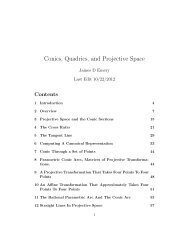
We haveOn the other handX T i KX j = X T i ω2 j MX j = ω 2 j XT i MX jSoX T i KX j = (K T X i ) T X j = (KX i ) T X j = (ω 2 i MX i ) T X j= ω 2 i X T i M T X j = ω 2 i X T i MX j .ω 2 jX T i MX j = ω 2 i X T i MX j .But ω j and ω i are not equal, so that we must haveand thenNow letX T i MX j = 0,X T i KX j = 0.X T i MX i = µ 2 i.Any multiple of an eigenvector is still an eigenvector, so we scale the eigenvectorsso that eachµ 2 i = 1ThenThen we haveP T MP = I.P T KP = P T MPΛ = IΛ = Λ.Both matrices have been diagonalized.28.3 Example: Coupled OscillatorsConsider two masses m 1 and m 2 . They can each move in a horizontal direction.Let the masses be connected with springs, k 1 , k 2 , and k 3 . Spring k 1is connected on the left with a fixed point, and on the right with mass m 1 .Spring k 2 is connected on the left with m 1 , and on the right with mass m 2 .Spring k 3 is connected on the left with m 2 , and on the right with a fixedpoint. Let u 1 and u 2 be the displacement from equilibrium of masses m 1 andm 2 respectively. The kinetic energy of the system is29

T = 1 2 m 1 ˙u 2 1 + 1 2 m 2 ˙u 2 2and the potential energy isThe Lagrangian isV = 1 2 k 1u 2 1 + 1 2 k 2(u 2 − u 1 ) 2 + 1 2 k 3u 2 2.L = T − V.The equations of motion are given by Lagrange’s equationsandWe haveandAlsoandThus Lagrange’s equations ared ∂L− ∂L = 0dt ∂ ˙u 1 ∂u 1d ∂L− ∂L = 0.dt ∂ ˙u 2 ∂u 2∂L∂ ˙u 1= ∂T∂ ˙u 1= m 1 ˙u 1∂L= ∂T = m 2 ˙u 2 .∂ ˙u 2 ∂ ˙u 2− ∂L∂u 1= ∂V∂u 1= k 1 u 1 − k 2 (u 2 − u 1 )− ∂L∂u 2= ∂V∂u 2= k 2 (u 2 − u 1 ) + k 3 u 2 .m 1 ü 1 + k 1 u 1 − k 2 (u 2 − u 1 ) = 0andm 2 ü 2 + k 2 (u 2 − u 1 ) + k 3 u 2 = 0.30

In matrix form the equations becomewhereandLetandThen[ ] [ ]ü1 u1M + K = 0ü 2 u 2K =M =[ ]m1 0,0 m 2[(k1 + k 2 ) −k 2−k 2 (k 3 + k 2 )u 1 = U 1 e iωtu 2 = U 2 e iωt .(K − ω 2 M)[u1u 2]= 0This equation has a nonzero solution if and only ifLet λ = ω 2 . The determinant isdet(K − ω 2 M) = 0.(k 1 + k 2 − λm 1 )(k 3 + k 2 − λm 2 ) − k 2 2 ,which we equate to zero to find the eigenvalues λ. Now let us specialize theproblem and set the spring constants k 1 and k 3 , to a common value k. Andalso set the two masses m 1 and m 3 , to a common value m. Let the couplingspring be a weak spring.That is, let spring constant k 2 be equal to a fraction of k. The equationfor the eigenvalues is the quadratic equation(k + k 2 − λm)(k + k 2 − λm) − k 2 2 = 0.].That is, it isAλ 2 + Bλ + C = 0,31

M1M2K1 K2 K3Figure 1: Coupled springs, With masses m 1 and m 1 . The spring constantsare k 1 , k 2 and k 3 . k 2 is the constant for the coupling spring and is muchsmaller than the other two constants.32

withandA = m 2B = −2(k + k 2 )mC = (k + k 2 ) 2 − k 2 2 = k2 + 2kk 2 .Let a = (k + k 2 − λm) and b = −k 2 . Then since the determinant is 0, wemust havea 2 = b 2So eitherora = b,a = −b.The equations for the eigenvectors areandIf a = b, then the eigenvector isaU 1 + bU 2 = 0,bU 1 + aU 2 = 0.[1−1]On the other hand, if a = −b, then the eigenvector is[11]The eigenvalues are λ 1 and λ 2 . Let a i be the value of a for eigenvalue λ i , andlet b i be the value of b for eigenvalue λ i . Now let us compute with values assignedto the constants. Let m = 1, k = 1, and k 2 = 1/10. The computationis done with a Matlab script (Octave script). Call it coupled.m:33

m=1.;k=1.;k_2=1/10;A= m*m;B= -2*(k+k_2)*m ;C= k^2 + 2 * k * k_2;lambda_1=(-B + sqrt(B*B - 4*A*C))/(2*A)omega_1=sqrt(lambda_1)a_1 = (k + k_2 - lambda_1 * m)b_1 = -k_2lambda_2=(-B - sqrt(B*B - 4*A*C))/(2*A)omega_2=sqrt(lambda_2)a_2 = (k + k_2 - lambda_2 * m)b_2 = -k_2omega=(omega_1+omega_2)/2t1=2*pi/omegaphi=(omega_1 -omega_2)/2t2=2*pi/phiThe output is:octave-3.0.0.exe:5> coupledlambda_1 = 1.2000omega_1 = 1.0954a_1 = -0.10000b_1 = -0.10000lambda_2 = 1.00000omega_2 = 1.00000a_2 = 0.10000b_2 = -0.10000omega = 1.0477t1 = 5.9970phi = 0.047723t2 = 131.66octave-3.0.0.exe:6> exitThe first eigenvalue isλ 1 = 1.234

a 1 and b 1 are equal, so the eigenvector is[1−1]The corresponding frequencies are√ω 1 = ± λ 1 = ±1.0954Hence two linearly independent solutions aree iω 1t[1−1]ande −iω 1t[1−1So any linear combination of these solutions is also a solution. That is, thespace spanned by these two solutions is a solution. But both cos(ω 1 t) andsin(ω 1 t) can be written as a linear combination of e iω 1t and e −iω 1t . Hencethis solution space is the same as the space spanned bycos(ω 1 t)][1−1.]andThe second eigenvalue is[1sin(ω 1 t)−1λ 2 = 1.0].a 2 and b 2 are not equal, so the eigenvector is[11]The corresponding frequencies are√ω 1 = ± λ 2 = ±1.035

Hence two linearly independent solutions are[ ]e iω 2t 11ande −iω 2t[11].Again the solution space is spanned by[1cos(ω 2 t)1]and[1sin(ω 2 t)1].Suppose the initial conditions areu 1 (0) = Adu 1 (0)= 0dtu 2 (0) = 0du 2 (0)dtLet the solution be[ ]1u = c 11 cos(ω 1 t) +c−1 12 sin(ω 1 t)[1−1= 0][1+c 21 cos(ω 2 t)1][1+c 22 sin(ω 2 t)1],where the constants are to be determined by the initial conditions.From the first initial condition we havec 11 + c 21 = AFrom the third initial condition we have−c 11 + c 21 = 036

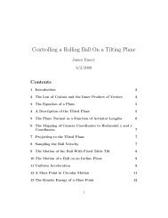
Figure 2: Coupled oscillations. The lower curve is the oscillation of mass m 1 .The upper curve is the oscillation of mass m 2 .37

Thusandc 21 = A/2c 11 = A/2.Differentiating our solution, we have[ ]du1dt = −c 11ω 1 sin(ω 1 t)−1+c 12 ω 1 cos(ω 1 t)From the second initial condition we havec 12 ω 1 + c 22 ω 2 = 0.From the forth initial condition we have[1−1−c 12 ω 1 + c 22 ω 2 = 0.Therefore c 22 = 0 and c 12 = 0. Therefore our solution is][1−c 21 ω 2 sin(ω 2 t)1][1+c 22 ω 2 cos(ω 2 t)1].u 1 = A 2 cos(ω 1t) + A 2 cos(ω 2t).u 2 = − A 2 cos(ω 1t) + A 2 cos(ω 2t).Now if ω = (ω 1 + ω 2 )/2 and φ = (ω 1 − ω 2 )/2, thencos(ω 1 t) + cos(ω 2 t) = 2 cos(ωt) cos(φt)SoSimilarlyu 1 = A cos(ωt) cos(φt).u 2 = −A sin(ωt) sin(φt).For the numbers we have used here the oscillating frequency isω = 1.0477,and the corresponding period isT 1 = 5.9970.38

The modulating frequency isφ = 0.047723,and the modulating period ist 2 = 131.66.The oscillators operate as follows. The first oscillator starts at maximumamplitude A, while the second oscillator is stopped at zero amplitude. Theamplitude of the first oscillator begins to decrease, according to the modulatingfactor cos(φt). At t = t 2 /4, the amplitude of the first oscillator hasdecreased to zero, whereas the amplitude of the second oscillator has increasedto its maximum amplitude A, according to the modulating factorsin(φt) . The energy of the first oscillator has been transferred to the second.This behavior repeats, as energy flows back and forth between the twooscillators.28.4 The General Problem of Linear VibrationThe reference for this section is:Bradbury T C, Theoretical Mechanics, John Wiley, 1968, p352.The kinetic and potential energies are given as quadratic formsT = 1 2 g ij ˙q i ˙q j ,andV = 1 2 k ijq i q j .The Lagrange equations of motion becomeg ij¨q j + k ij q j = 0.Write this as a matrix equationG ¨Q + KQ = 0,where G and K are symmetric n by n matrices. This equation has a solutionQ = X exp(ωt).39

Thenwhere(K − λG)X = 0,λ = ω 2 .This is a generalized eigenvalue problem. The quadratic forms are positivedefinite. The eigenvalues are real, and the eigenvectors (normal modes) areorthogonal. Let the rows of matrix S be constructed out of eigenvectors,which are scaled to be of unit length with metric G (S, or S T is called themodal matrix in Thomson ”Theory of Vibration.”). That is,ThenX T GX = δ ij .SGS T = I.Let Λ be a diagonal matrix of the eigenvalues. ThenDefine normal coordinates Q ′ byThen the equations of motion becomeKS T = ΛGS.Q = Q ′ S T .GS T ¨Q′ + KS T Q ′ = 0.Multiplying by S and simplifying, we get¨Q ′ + ΛQ ′ = 0.The problem could also be solved by diagonalizing the original energy quadraticforms. Any two positive definite quadratic forms can be simultaneously diagonalized.See for example, D. E. Littlewood A University Algebra, 2nded. 1958 Dover, p53.40

29 Polynomial Roots, The Frobenius CompanionMatrixThe roots of a polynomial p(x) can be computed as the eigenvalues of theFrobenious companion matric. This is because p(x) is the characteristic polynomialof the companion matrix, which can be proved using mathematicalinduction. See MatLab help for the polynomial roots function, called roots.For example if p(x) is a third degee polynomial, thenp(x) = c 0 + c 1 x + c 2 x 2 + x 3 ,Then the companion matrix is the following 3 × 3 matrix:⎡ ⎤0 0 −c 0⎢ ⎥⎣ 1 0 −c 1 ⎦0 1 −c 2The characteristic polynomial is−λ 0 −c 01 −λ −c 1∣ 0 1 −c 2 − λ ∣= −λ∣−λ −c 11 −c 2 − λ∣ − c 0∣= −c 0 − λ(c 1 + c 2 λ + λ 2 )= −c 0 − c 1 λ − c 2 λ 2 − λ 3 ,1 −λ0 1by induction. And so it goes.Notice that if n is odd then the characteristic equation computed fromthe companion matrix gives−(c 0 + c 1 λ + c 2 λ 2 + ... + λ n )whereas if n is even then the characteristic equation computed from thecompanion matrix givesc 0 + c 1 λ + c 2 λ 2 + ... + λ n ,which takes care of the alternating signs in Cramers rule in the inductionstep.41∣

were rational we could write √32 = n m ,30 Projection OperatorsA projection operator is a linear operator P that has the property thatP(P(v)) = P(v).So for example in the simple geometric case of projecting a 3-d vector to a2-d subspace, that is to a plane, the projection then lies in the plane, henceprojecting it again to the plane does not alter it because it is already in theplane.31 Functional AnalysisWhen our vector spaces are infinite dimensional, for example consider thevector space of all continuous functions on an interval [a, b], we enter therealm of functional analysis. This area of mathematics arose out of the problemsof solving differential and integral equations, and in such areas as FourierAnalysis. So one studies Hilbert Spaces, which are complete inner productspaces, and Banach Spaces, which are complete normed linear spaces. In afurther increase in abstraction one studies Topological Vector spaces in whichthere may be no inner product or norm.32 Hamel BasisHamel constructed a basis for the vector space of real numbers over therational field. He did this using Zorn’s Lemma. So for example the vectors√2 and√3 are linearly independent. Otherwise√32would be a rational number.For if we assumed that √3242

where n and m have no common factor. Then32 = n2m 2,3m 2 = 2n 2 ,so n 2 and thus n must have a factor of 3. Hence m 2 and hence m must havea factor of 3. This contradicts our assumption.See Angus Taylor Introduction to Functional Analysis for a treatmentof Hamel basis.33 Numerical Linear AlgebraSee Golub and Van Loan, and books on Matlab.34 Quantum MechanicsQuantum Mechanics was treated by John Von Neumann in terms of HilbertSpaces and Linear Operators in Hilbert Space, and involving eigenvalues andeigenvectors of such spaces of functions. One runs into things like delta functions,which are approximations to functions, but not actually functions atall. Thus we use mathematical objects called distributions. These distributionsare functionals and not to be confused with probability distributions.Von Neumann made great contributions to the study of Banach Algebras.35 The Schrodinger Wave EquationFrom the photoelectric effect, the energy of a photon isE = hν,where h is Planck’s constant, and ν is the frequency of the photon. Fromrelativity theory, the energy of a particle is given by the equationE 2 = p 2 v 2 + m 2 c 4 ,43

where v is the particle velocity and m is its mass. For a photon the velocityis the velocity of light c, and the mass is zero. Thus for a photonThis implies that the wavelength isE 2 = p 2 c 2 .λ = c/ν = E/pE/h = h/p.Let k be the wave number vector. By definitionkλ = 2π.We havewhereA plane wave takes the formp = khkλ = ¯hk,¯h = h2π .e i(k·r−ωt) = e (i/¯h)(p·r−Et)A wave packet is represented as a sum of such plane waves, written as theFourier transformψ(r, t) = √ 1 ∫a(p)e (i/¯h)(p·r−Et) dp.2πhThis wave function satisfies the equation(¯h 2 /2m)∇ 2 ψ − (¯h/i)∂ψ/∂t = 0,because p 2 /(2m) − E = 0. It is called the Schrodinger wave equation. Thegroup velocity of the wave packet isv g = dωdk = dEdp .44

UsingandE =p =mc 2√1 − v 2 /c 2,mv√1 − v 2 /c 2.We find thatdEdp = pc2E = v.Thus the group velocity of the wave packet corresponds to the particle velocity.|ψ 2 | is proportional to the probability density function for the locationof the particle. This is the Born postulate.36 The Postulates of Quantum MechanicsThe dynamical variables of a mechanical system are interpreted as operators,operating on wave functions which are elements of a Hilbert space. Theidentification with classical mechanics is done somewhat in the manner ofthe mathematical theory of distributions. The expected values of a variable(i.e. the measured values) form a discrete set which is the set of eigenvaluesof the operator.37 The Bra and Ket Notation of DiracA ket v > vector is an element of a Hilbert space (a complete complex innerproduct space). A bra vector < u is an element of the dual space, that is, itis a linear operator. Thus the value of u on v isu(v) =< u|v >,which also may be interpreted as an inner product.In another way of looking at it, a bra vector < v is a row matrix ofcomponents with respect to some basis, of a vector v, that is ifn∑v = v i b ii=145

thenv >= [ v 1 v 2 ... v n]and a ket vector v > is the conjugate transpose, and thus a column vectorof components.From a mathematical point of view, this bra and ket business seems rathercomplicated, confused, and is not clearly necessary.Chapter VII in Messiah outlines some linear algebra in this bra ket notation.Section 2.3 of Shankar gives another explanation of this notation.38 Example: The Hydrogen AtomSchrodinger’s equation is a partial differential equation and can be solved bythe method of separation of variable. That is a solution can be written asa product, where each product function uses independent variables. Thenusually the partial differential equation becomes a set of ordinary differentialequations and eigenvalue problems. These eigenvalues than characterizequantum energy levels. In the case of the hydrogen atom,39 The Relation Between Linear Algebra, FunctionalAnalysis, and Abstract Solutions toProblemsUltimately the solution of applied problems must involve a finite set of numbersrather than an abstract infinite theoretical solution. But the abstractsolution can define properties of the solution and indeed existence of a solutionand uniqueness. This is important, for finite approximations of a solutionthat does not exist will fail. So finally we typically will use the resultsof linear algebra to find arbitrary close approximations to applied problems.Specifically we require results from numerical linear algebra. That is we needalgorithms that are robust, accurate, and render roundoff and truncation errorsmall.46

40 BibliographyThe number of books written on linear algebra and functional analysis ishuge. So I list here some favorites of mine.[1] Lange Serge, Linear Algebra Addison Wesley, 1968[2]Lawson and Hanson, Solving Linear Least Squares Problems, (JEL),1974, (least squares, singular value decomposition).[3]Stoker J J, Nonlinear Vibrations, (JEL).[4]Akhiezer N I, Glazman I M, Theory of Linear Operators in HilbertSpace, V I 1961, V II 1963, (two volumes Dover 1993).[5]Halmos Paul R, Finite-Dimensional Vector Spaces, Springer-Verlag,1974.[6]Halmos Paul R, Introduction to Hilbert Space and the Theory ofSpectral Multiplicity, 2nd ed., Chelsea, 1951.[7]Herstein I N, Topics in Algebra, Blaisdell, 1964., (Frobenius Theoremon Division Algebras, Quaternions).[8]Strang Gilbert, Linear Algebra and Its Applications, Academic Press,1980, 2nd Edition..[9]Fausett Laurene V, Applied Numerical Analysis Using Matlab, Prentice-Hall, 1999..[10]Golub Gene H, Van Loan Charles F, Matrix Computations, John HopkinsUniversity Press, 1989.[11]Lorch Edward R, The Spectral Theorem, In Studies in Modern AnalysisVolume I, R. C. Buck editor, MAA Studies in Mathematics, The MathematicalAssociation of America, 1962.[12]Taylor Angus E, Introduction to Functional Analysis, John Wiley,1967.[13]Courant Richard, Hilbert David, Methods of Mathematical Physics,Volumes I and 2, Wiley, Springer , 1937.[14]Bamberg Paul, Sternberg Shlomo, A Course in Mathematics for Studentsof Physics,, volumes 1 and 2 , Cambridge University Press, 1988..[15]Yosida Kosaku, Functional Analysis, 2nd Edition, 1968, Springer-Verlag.[16]Reed Michael, Simon Barry, 1972,, Methods of Modern MathematicalPhysics, Part 1. Functional Analysis, 1972, Academic Press.[17]Banach Stefan, Theorie Des Operations Lineares, Chelsea, 1932.[18]Banach Stefan, Theory of Linear Operations, English translation by47

F. Jellett, 1987, Elsevier..[19]Noble Ben, Applied Linear Algebra, Prentice-Hall 1969.[20]Nering Evar D, Linear Algebra and Matrix Theory, John Wiley,1963.[21]Powell John L, Crasemann Bernd Quantum Mechanics Addison-Wesley,1965.48