Math 2040 Matrix Theory and Linear Algebra II sample midterm ...
Math 2040 Matrix Theory and Linear Algebra II sample midterm ...
Math 2040 Matrix Theory and Linear Algebra II sample midterm ...

You also want an ePaper? Increase the reach of your titles
YUMPU automatically turns print PDFs into web optimized ePapers that Google loves.
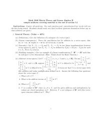
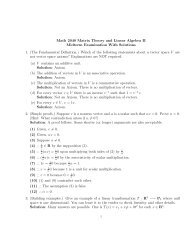
<strong>Math</strong> <strong>2040</strong> <strong>Matrix</strong> <strong>Theory</strong> <strong>and</strong> <strong>Linear</strong> <strong>Algebra</strong> <strong>II</strong><br />
<strong>sample</strong> <strong>midterm</strong> covering material to the end of section 5.1<br />
Instructions: Answer all questions. For each question part, parenthesized key words tell you<br />
the idea being tested. (Students should work very hard on these questions themselves before any in<br />
class solutions are given.)<br />
1. General <strong>Theory</strong>. (Value = 40%)<br />
(a) (Definitions.) Give the definition of a subspace of a vector space.<br />
Solution: A subspace of a vector space V is a nonempty subset W of V such that W is<br />
closed under the operations of addition <strong>and</strong> scalar multiplication on V .<br />
(b) (Axiom consequences.) Prove the cancellation law for addition in a vector space; that<br />
u + v = u + w implies v = w for all vectors u, v <strong>and</strong> w.<br />
Solution:<br />
(1) u + v = u + w by assumption.<br />
(2) ∴ −u + (u + v) = −u + (u + w) upon adding −u to both sides of (1).<br />
(3) ∴ (−u + u) + v = (−u + u) + w because addition of vectors is associative.<br />
(4) ∴ 0 + v = 0 + w because −u + u = 0, −u being the additive inverse of u.<br />
(5) ∴ v = w because 0 is a unit for vector addition.<br />
(c) (<strong>Linear</strong>ity.) Let T 1 : V 1 −→ V 2 <strong>and</strong> T 2 : V 1 −→ V 2 be two linear transformations between<br />
vector spaces V 1 <strong>and</strong> V 2 . Let T 3 : V 1 −→ V 2 be defined by T 3 (v) = 2T 1 (v) − T 2 (v) for each<br />
v ∈ V 1 . Prove T 3 is linear.<br />
Solution: Let u, w ∈ V 1 <strong>and</strong> let α, β ∈ R. We will show T 3 (αu + βw) = αT 3 (u) + βT 3 (w).<br />
(1) T 3 (αu + βw) = 2T 1 (αu + βw) − T 2 (αu + βw) by the definition of T 3 .<br />
(2) ∴ T 3 (αu + βw) = 2αT 1 (u) + 2βT 2 (w) − αT 2 (u) − βT 2 (w) because T 1 <strong>and</strong> T 2 are linear,<br />
<strong>and</strong> because 2 is a scalar (so, multiplication by 2 distributes over addition).<br />
(3) ∴ T 3 (αu + βw) = 2αT 1 (u) − αT 2 (u)) + 2βT 2 (w) − βT 2 (w) by a simple rearrangement<br />
of terms using commutativity of addition.<br />
(4) ∴ T 3 (αu+βw) = α(2T 1 (u)−T 2 (u)))+β(2T 2 (w)−T 2 (w)) because scalar multiplications<br />
by α <strong>and</strong> β distribute over vector additions.<br />
(5) ∴ T 3 (αu + βw) = αT 3 (u) + βT 3 (w) as required.<br />
(d) (Building examples.) Give an example of a linear transformation T : R 3 −→ R 3 such that<br />
its null space is two dimensional. (Hint: Think about the Rank Theorem.)<br />
Solution: There are many possibilities. Any 3 × 3 matrix with rank 1 will do, say, the<br />
matrix [e 1 e 1 e 1 ].<br />
1
[ ]<br />
[ ]<br />
r1<br />
x1<br />
(e) (Abstract vector spaces.) Let V = { | r<br />
r 1 +r 2 = 1 <strong>and</strong> r 1 , r 2 ∈ R}. For any ∈ V ,<br />
2 x<br />
[ ]<br />
[ ] [ ]<br />
[ 2<br />
]<br />
y1<br />
x1 y1<br />
x1 + y<br />
∈ V , <strong>and</strong> α ∈ R, suppose + in V is defined to be<br />
1 − 1<br />
<strong>and</strong><br />
y 2 x 2 y 2 x 2 + y<br />
[ ]<br />
[ ]<br />
2<br />
x1<br />
αx1 + (1 − α)<br />
α in V is defined to be<br />
. It turns out that V is a vector space with<br />
x 2 αx 2<br />
this addition <strong>and</strong> scalar multiplication defined on it. Answer the following four questions<br />
about the vector space V .<br />
i. What is 0 ∈ V [<br />
]<br />
1<br />
Solution: 0 = in V .<br />
0<br />
[ ]<br />
4<br />
ii. What is the additive inverse of in V <br />
−3<br />
[ ]<br />
[ ] [ ]<br />
−2 4<br />
1<br />
Solution: , since adding this to results in .<br />
3<br />
−3<br />
0<br />
[ ]<br />
4<br />
iii. What is 5 in V <br />
−3<br />
[ ] [ ]<br />
5(4) + (1 − 5)<br />
16<br />
Solution:<br />
; that is, .<br />
5(−3)<br />
−15<br />
iv. V is a subset of R 2 , there is a 0 ∈ V , <strong>and</strong> the given addition <strong>and</strong> multiplication by<br />
scalars are closed operations on V . However, V a not subspace of R 2 with this vector<br />
space structure defined on [ V . Why ]<br />
0<br />
Solution: The 0 ∈ R 2 is , but this is not in V . Also, the addition <strong>and</strong> scalar<br />
0<br />
multiplication given for V does not correspond to addition <strong>and</strong> scalar multiplication<br />
inherited from R 2 .<br />
2. Representations. (Value = 40%)<br />
Let B = {b 1 , b 2 , b 3 } be a basis of a vector space V . Let<br />
c 1 = b 1 + b 2 ,<br />
c 2 = b 2 + b 3 , <strong>and</strong><br />
c 3 = b 1 + b 3 .<br />
Let C = {c 1 , c 2 , c 3 }.<br />
(a) (Coordinates.) If [x] B =<br />
⎡<br />
⎣ −1 1<br />
−2<br />
⎤<br />
⎦, then what is x<br />
Solution: x = −b 1 + b 2 − 2b 3<br />
2
(b) (Basis <strong>and</strong> isomorphism.) Prove C is a basis of V by considering {[c 1 ] B , [c 2 ] B , [c 3 ] B } in R 3 .<br />
What about P B allows this consideration<br />
Solution: P B : R 3 → V is an isomorphism of vector spaces, so C is a basis of V ⎡if <strong>and</strong> ⎤<br />
only if {[c 1 ] B , [c 2 ] B , [c 3 ] B } is a basis of R 3 . [c 1 ] B = [b 1 + b 2 ] B = [b 1 + b 2 + 0b 3 ] B = ⎣ 1 1<br />
0<br />
⎡ ⎤<br />
⎡<br />
⎦.<br />
⎤<br />
Similarly, by inspection of the given equations, we have [c 2 ] B = ⎣ 0 1 ⎦, <strong>and</strong> [c 3 ] B = ⎣ 1 0 ⎦.<br />
1<br />
1<br />
{[c ⎡ 1 ] B , [c 2 ] B , [c 3 ] B } is a basis of R 3 since an easy row reduction shows the 3 × 3 matrix<br />
⎣ 1 0 1<br />
⎤<br />
1 1 0 ⎦ has 3 pivot columns. Therefore, C is a basis of V as required.<br />
0 1 1<br />
(c) (Change of coordinates.) Calculate the change-of-coordinate matrix P C←B from B represented<br />
vectors to C represented vectors. (Hint: Think about P B←C instead <strong>and</strong> its relationship<br />
to P C←B .)<br />
Solution. P B←C = [[c 1 ] B [c 2 ] B [c 3 ] B }] =<br />
⎡<br />
⎡<br />
⎣ 1 0 1<br />
1 1 0<br />
0 1 1<br />
⎤<br />
⎤<br />
⎦. P C←B = P −1<br />
B←C<br />
, so it is simply a matter<br />
of computing the inverse of ⎣ 1 0 1<br />
1 1 0 ⎦. I will not waste time doing this as I am sure all<br />
0 1 1<br />
M<strong>2040</strong> students can calculate the inverse.<br />
(d) (<strong>Linear</strong>ity.) Let T : V −→ V be a linear transformation <strong>and</strong> [T ] B ⎡be the ⎤ representation<br />
of T relative to the basis B. Assume, the first column of [T ] B is<br />
T (2b 2 ) = 2b 1 + 4b 2 + 2b 3 <strong>and</strong> [T ] B<br />
⎡<br />
⎣ 1 1<br />
1<br />
i. What is the second column of [T ] B <br />
ii. What is the third column of [T ] B <br />
⎤<br />
⎦ =<br />
⎡<br />
⎣ 1 0<br />
3<br />
⎤<br />
⎦.<br />
⎣ 1 0<br />
6<br />
⎦. Also, suppose<br />
Solution. By linearity, T (b 2 ) = b 1 + 2b 2 + b 3 . So now⎡the ⎤second column of [T ] B is<br />
[T ] B e 2 = (P −1<br />
B<br />
T P B)e 2 = P −1<br />
B<br />
T (b) 2 = P −1<br />
B (b 1 + 2b 2 + b 3 ) =<br />
⎣ 1 2<br />
1<br />
⎦.<br />
3
Next, [T ] B<br />
⎡<br />
⎣ 1 1<br />
1<br />
⎤<br />
[T ] B (e 3 ). Therefore,<br />
[T ] B (e 3 ) =<br />
⎡<br />
⎣ −1<br />
−2<br />
−4<br />
⎦ = [T ] B (e 1 + e 2 + e 3 ) = [T ] B (e 1 ) + [T ] B (e 2 ) + [T ] B (e 3 ) =<br />
⎤<br />
⎦.<br />
⎡<br />
⎣ 1 0<br />
3<br />
⎤<br />
⎦ =<br />
⎡<br />
⎣ 1 0<br />
6<br />
⎤<br />
⎦ +<br />
⎡<br />
⎣ 1 2<br />
1<br />
⎤<br />
⎡<br />
⎣ 1 0<br />
6<br />
⎤<br />
⎦ +<br />
⎡<br />
⎣ 1 2<br />
1<br />
⎤<br />
⎦ +<br />
⎦ + [T ] B (e 3 ) <strong>and</strong> this gives us the third column,<br />
(e) (Diagram chasing.) Let T be as in the last part d) above. For 7 test points, write a matrix<br />
equation expressing [T ] C in terms of the symbols P C←B , [T ] B , <strong>and</strong> P B←C . For 1 test point,<br />
use this equation to find the matrix [T ] C .<br />
Solution. [T ] C = P C←B [T ] B P B←C . I won’t bother with the matrix multiplications which I<br />
am confident all M<strong>2040</strong> students can do.<br />
3. Eigenvalues <strong>and</strong> Eigenvectors. ⎡<br />
(Value = 20%)<br />
Let A be the matrix ⎣ 4 −1 6<br />
⎤<br />
2 1 6 ⎦.<br />
2 −1 8<br />
(a) (Eigenvalues.) Show⎡λ = 2 is an eigenvalue of A (do not use the characteristic polynomial).<br />
Solution. A − 2I = ⎣ 2 −1 6<br />
⎤ ⎡<br />
2 −1 6 ⎦ ∼ ⎣ 2 −1 0<br />
⎤<br />
0 0 1 ⎦, so Nul(A − 2I), the eigenspace of A<br />
2 −3 8 0 0 0<br />
corresponding to λ = 2, is nontrivial. Therefore, λ = 2 is an eigenvalue of A.<br />
(b) (Eigenvalues.) Show λ = 1 is not an eigenvalue of A (again, do not use the characteristic<br />
polynomial).<br />
⎡<br />
Solution. A − I = ⎣ 3 −1 6<br />
⎤ ⎡<br />
⎤<br />
1 0 2<br />
2 0 6 ⎦ ∼ ⎣ 0 1 0 ⎦, so Nul(A − 2I), the eigenspace of A<br />
2 −3 7 0 0 1<br />
corresponding to λ = 2, is trivial. Therefore, λ = 2 is an eigenvalue of A.<br />
⎡ ⎤<br />
(c) (Eigenvectors.) Is ⎣ 1 1 ⎦ an eigenvector of A If so, then what is its corresponding eigenvalue<br />
<strong>and</strong>, if not, ⎡then⎤<br />
why ⎡not<br />
1<br />
⎤<br />
Solution. Yes, A<br />
⎣ 1 1<br />
1<br />
⎦ = 8<br />
⎣ 1 1<br />
1<br />
⎦, so the corresponding eigenvalue is λ = 8<br />
4
⎡<br />
⎤<br />
(d) (Eigenvectors.) Is ⎣ 1 1 ⎦ an eigenvector of A If so, then what is its corresponding eigenvalue<br />
<strong>and</strong>, if not, ⎡then ⎤ why ⎡ not ⎤ ⎡<br />
0<br />
⎤<br />
Solution. No, A<br />
⎣ 1 1<br />
0<br />
⎦ =<br />
⎣ 3 3<br />
12<br />
⎦ ≠ λ<br />
⎣ 1 1<br />
0<br />
⎦ for any λ ∈ R 2 .<br />
(e) (Eigenspace.) Find a basis of the ⎡ eigenspace corresponding to λ = 2.<br />
Solution. Nul(A − 2I) = Nul( ⎣ 1 −1/2 0<br />
⎤ ⎡<br />
0 0 1 ⎦) = Span{ ⎣ 1/2 ⎤<br />
1 ⎦}. Therefore, a basis of<br />
0 0 0<br />
0<br />
⎡ ⎤<br />
the eigenspace of λ = 2 is { ⎣ 1 2<br />
0<br />
⎦}.<br />
End Midterm.<br />
5