A two-fluid model of turbulent two-phase flow for simulating turbulent ...

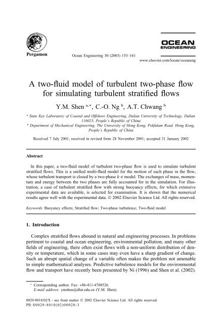
Ocean Engineering 30 (2003) 153–161
www.elsevier.com/locate/oceaneng
A two-fluid model of turbulent two-phase flow
for simulating turbulent stratified flows
Y.M. Shen a,∗ , C.-O. Ng b , A.T. Chwang b
a
State Key Laboratory of Coastal and Offshore Engineering, Dalian University of Technology, Dalian
116023, People’s Republic of China
b
Department of Mechanical Engineering, The University of Hong Kong, Pokfulam Road, Hong Kong,
People’s Republic of China
Received 7 July 2001; received in revised form 28 November 2001; accepted 31 January 2002
Abstract
In this paper, a two-fluid model of turbulent two-phase flow is used to simulate turbulent
stratified flows. This is a unified multi-fluid model for the motion of each phase in the flow,
whose turbulent transport is closed by a two-phase k–e model. The exchanges of mass, momentum
and energy between the two phases are fully accounted for in the simulation. For illustration,
a case of turbulent stratified flow with strong buoyancy effects, for which extensive
experimental data are available, is selected for examination. It is shown that the numerical
results agree well with the experimental data. © 2002 Elsevier Science Ltd. All rights reserved.
Keywords: Buoyancy effects; Stratified flow; Two-phase turbulence; Two-fluid model
1. Introduction
Complex stratified flows abound in natural and engineering processes. In problems
pertinent to coastal and ocean engineering, environmental pollution, and many other
fields of engineering, there often exist flows with a non-uniform distribution of density
or temperature, which in some cases may even have a sharp gradient of change.
Such an abrupt spatial change of a variable often makes the problem not amenable
to simple mathematical analyses. Predictive turbulence models for the environmental
flow and transport have recently been presented by Ni (1996) and Shen et al. (2002).
∗
Corresponding author. Fax: +86-411-4708526.
E-mail address: ymshen@dlut.edu.cn (Y.M. Shen).
0029-8018/02/$ - see front matter © 2002 Elsevier Science Ltd. All rights reserved.
PII: S 00 29 -8018(02)00020-3

154 Y.M. Shen et al. / Ocean Engineering 30 (2003) 153–161
Nomenclature
C 1
C 2
C m
F
g
k
K f
K m
P
R
t
U
X
e
m
m e
m t
ρ
s k
s e
s
a turbulence coefficient constant
a turbulence coefficient constant
a turbulence coefficient constant
time-averaged frictional force
gravitational acceleration
turbulent kinetic energy
an empirical constant
an empirical constant
time-averaged pressure
a generic variable
time
time-averaged velocity
Cartesian coordinate
turbulent kinetic energy dissipation rate
dynamic viscosity
effective dynamic viscosity
dynamic eddy viscosity
substance density
a turbulence coefficient constant
a turbulence coefficient constant
a turbulence coefficient constant
time-averaged volume fraction
Subscripts
1 first phase
2 second phase
i component in the i direction
k phase k
l phase l
r ambient fluid
rel relative value
These models have made some success. However they do not account for the mixing
structure of a flow field in sufficiently fine detail. A problem that is characterized
by appreciable phase exchanges of mass, momentum and energy can be too complicated
to be accurately simulated by a simple turbulence closure model. It is of practical
importance if a model is able to distinguish the various components of a flow
field in the course of simulation. Spalding (1984) proposed a two-fluid model of

Y.M. Shen et al. / Ocean Engineering 30 (2003) 153–161
155
turbulence (see also Markatos, 1985), which was later improved by Fan (1988). A
distinct feature of the model is to treat a general phase as a substance that can be
distinguished by a property parameter such as temperature, pressure, velocity, density,
and so on. Based on the framework of the two-fluid model, it is the intention
of this work to present a two-fluid model of turbulent two-phase flow for the simulation
of turbulent stratified flows. Computational results are shown to agree well
with some published experimental data.
2. Physical concepts
A central part of the two-fluid model of turbulent two-phase flow is to consider
such flow being composed of the interacting turbulent motions of two fluids, which
coexist in time and space but possess different volume fractions. These two fluids
in turbulent motion can be regarded as interpenetrating continua, which obey their
own governing differential equations. The two fluids can have exchanges of mass,
momentum and energy with each other. For identification, each fluid carries a distinct
phasal mark that remains invariant throughout the flow. Let k 1 and k 2be
used to mark the two different fluids in the flow. Then the related properties of such
atwo-fluid model can be expressed in the following sections.
2.1. Mixture parameters of two-phase flow
Any parameter for a mixture of two phases can be obtained by taking a weighted
average of the corresponding parameters for each phase. The volume-average and
mass-average are the two typical ways of deriving the parameters of the mixture,
which are defined as follows:
Volume-average:
R 1 R 1 2 R 2 (1)
Mass-average:
R ( 1 r 1 R 1 2 r 2 R 2 )/r (2)
r 1 r 1 2 r 2 (3)
where 1 and 2 are respectively the volume fractions of the first and second phases,
r 1 and r 2 are the respective substance densities of the two phases, and R is a generic
variable that can be the velocity, turbulence properties, and so on.
2.2. Pressure of two-phase flow
There are two alternative ways of defining the mixture pressure of two-phase flow.
By the first definition, the mixture pressure is assumed to be composed of partial
pressures due to individual phases. It is further assumed that the partial pressure of
a phase amounts to the total pressure multiplied by the phase volume fraction k .

156 Y.M. Shen et al. / Ocean Engineering 30 (2003) 153–161
This concept is parallel to that of a gas mixture. The phase pressure P k and the total
pressure P are therefore related by:
P k
P k (P k P k ) (4)
Alternatively, the same pressure is assumed for each phase and the mixture, i.e.
P k (k 1,2) P. The phasal pressure gradient in the momentum equation is, however,
the pressure gradient weighted by the volume fraction. These two ways of
defining the mixture pressure are related to each other if the contribution to the
pressure gradient is expressed as:
d Pi a P P ∂ k ∂P
∂X
k (5)
i ∂X i
When a P 1, d Pi ∂(P k )/∂X i ∂P k /∂X i , which is the former way. When
a P 0, then d Pi k ∂P/∂X i , which corresponds to the latter way. For convenience,
the second way of defining the mixture pressure is adopted in this paper,
i.e. a P 0.
3. Mathematical model
On applying the Reynolds decomposition and averaging to the instantaneous Navier–Stokes
equations, while modeling the correlation terms with a gradient-flux closure,
we obtain the governing equations that describe the transport of averaged parameters
in a turbulent two-phase flow system.
The time-averaged continuity equation (volume fraction equation) for phase k is
∂
∂t (r k k ) ∂ (r
∂X k k U kj ) ∂
j
∂X j l
s k
k
m el
m ek
The time-averaged momentum equation for phase k is
s l ∂ k
∂X j S k,l m k,l (6)
∂
∂t (r k k U ki ) ∂
∂X j
(r k k U kj U ki ) ∂
∂X j m ek
s kU kj
∂ k
∂X i
U ki
∂ k
∂X j (7)
∂
∂X j k m ek ∂U ki
∂X j
∂U kj
∂X i k
∂R
∂X i
k (r k r r )g i F ki
The transport equation of turbulent kinetic energy for phase k is
∂
∂t (r k k k k ) ∂
∂X j
(r k k U kj k k ) ∂
∂X j m ek
s kk
k
∂k k
∂X j ∂
∂X j m ek
s k
k k
∂ k
∂X j (8)
r k k e k G k B k a f m ek∂U ki
m el∂U li
s Uk ∂X i s Ul ∂X i

Y.M. Shen et al. / Ocean Engineering 30 (2003) 153–161
157
The transport equation of turbulent kinetic energy dissipation rate for phase k is
where
∂
∂t (r k k e k ) ∂
∂X j
(r k k U kj e k ) ∂
∂X j m ek
s ek
k
∂e k
∂X j ∂
∂X j m ek
s k
e k
∂ k
∂X j (9)
e k
k k
(C 1 G k C 2 r k k e k )2a f re k
F ki K f r k l |U ki U li |(U ki U li )e/k 1.5 (10)
S k,l E K m r k l |U ki U li |e/k 1.5 (11)
m k,l m el
s l
m ek
s k ∂ k
∂ l
(12)
∂X j ∂X j
G k ∂U ki
∂X j m ek
s k
U kj
∂ k
∂X i
m ek k ∂U ki
∂X j
∂U kj
∂X i (13)
B k m ek
s k r kr r
∂ k
g
∂X i (14)
i
r k
a f 1 r K fE (15)
k 2 k
m tk r k C m
e k
(16)
m ek m k m tk (17)
In the equations presented above, the symbols have the following meanings: t is
time; subscripts k and l are the fluid marks which may be either 1 or 2 (but k l);
F ki is the component of the time-averaged frictional force of phase k in the i direction;
U ki and U li are the components of the time-averaged velocity of phases k and l in
the i direction, respectively; k and l are the time-averaged volume fractions of
phases k and l, respectively; r, k and e are the density, turbulent kinetic energy and
turbulent kinetic energy dissipation rate of mixture, respectively; P is the time-averaged
pressure of the mixture; m k , m tk and m ek are the dynamic viscosity, dynamic
eddy viscosity and effective dynamic viscosity of phase k, respectively; r k is the
substance density of phase k; r r is the substance density of ambient fluid; s k is the
turbulent Schmidt number of phase k (which is constant in general, but strongly
influenced by buoyancy effects that can be accounted for with the Munk–Anderson
empirical formula, Rodi, 1993); g i is the component of gravitational acceleration in
the i direction; K f , K m , s kk , s ek , C 1 , C 2 and C m are all empirical constants for which
the following values are chosen: K f 0.05, K m 0.1, s kk 1.0, s ek
1.3, C 1 1.44, C 2 1.92 and C m 0.09.

158 Y.M. Shen et al. / Ocean Engineering 30 (2003) 153–161
4. Numerical computation and discussion on results
Atwo-fluid model system is obviously much more complex to compute than a
one-fluid system. For one thing, the number of differential equations for a two-fluid
model is twice that for a one-fluid model. Also, the non-linearity and coupling of
the equations are much stronger owing to interactions between the two fluids. The
equations are coupled not only within those for the same phase, but also among
those for different phases. On the other hand, the solution to the coupled equations
is highly sensitive to the initial values. Numerical efficiency is also strongly affected
by the methods for discretization and iteration, and the way of relaxation. These
computational difficulties can be mitigated only through taking good care of the nonlinearity
and coupling. In this regard, the numerical method that approaches the twofluid
system from a no-slip one-fluid system is used.
A unified multi-fluid model is adopted here, and the two-phase flow can be computed
by finite differences in a unified Eulerian field. In this work, the second-order
implicit SIMPLE scheme is extended to the two-phase flow. The pressure correction
equations are obtainable from the continuity equation for the mixture. By treating a
two-fluid system from the approach of a no-slip one-fluid system, the two-phase
coupling system is numerically solved with an under-relaxation iterative scheme.
4.1. Numerical example
The two-fluid model described above is applied to a problem as shown in Fig. 1,
for which the extensive data available from Uittenbogaard (1988) can be used for
comparison. In the experiment, a turbulent mixing layer was created between two
streams of water, initially separated by a splitter plate, having different velocities
and salinity concentrations. The two streams were maintained at a constant (and
equal) temperature but with a density difference of 15 kg/m 3 . The denser stream was
below the lighter one, a condition that gives rise to stable stratification leading to
suppression of turbulent mixing. This flow problem was adopted as a test case for
‘The Fourteenth Meeting of the IAHR Working Group on Refined Flow Modelling’
(Scheuerer, 1989).
The boundary conditions at the inlet cross-section, comprising profiles of the
dependent variables, were specified in the experiment, while at the exit the flow was
already fully developed. The top was a slip plane (rigid-lid approximation) and the
Fig. 1.
Flow geometry and coordinate system.

Y.M. Shen et al. / Ocean Engineering 30 (2003) 153–161
159
Fig. 2.
Computed and measured profiles of velocity of the mixture.
Fig. 3.
Computed profiles of velocities of the two fluids.
bottom was a smooth wall where the velocity follows a standard log-law and turbulence
is in local equilibrium.
4.2. Computational results and discussion
Comparisons between the computed and the measured profiles of velocity U, turbulent
kinetic energy k, and relative density r rel (rr 1 )/(r 2 r 1 ) for the mixture
are presented in Figs. 2, 4 and 6. The computed profiles of velocity U and turbulent
kinetic energy k for the two fluids are shown in Figs. 3 and 5. These profiles are
located at 5, 10 and 40 m downstream of the splitter plate. Clearly, the predictions
for the velocity and relative density are in very close agreement with the data in all
stages of the flow development. It is reproduced in the computation that the initially
Fig. 4.
Computed and measured profiles of turbulent kinetic energy of the mixture.

160 Y.M. Shen et al. / Ocean Engineering 30 (2003) 153–161
Fig. 5.
Computed profiles of turbulent kinetic energy of the two fluids.
Fig. 6.
Computed and measured profiles of the relative density.
distinct boundary layers that were developed on either side of the splitter plate have
almost merged into a single shear layer akin to a boundary layer developing over
the flume’s bed. The predictions also clearly show that the turbulent kinetic energy
has completely collapsed in the outer part of the shear layer under the influence of
strong stable stratification.
It is also apparent from the velocity and relative density profiles that the presence
of buoyancy makes the phase coupling to be of the ‘check type’, i.e. the phase
coupling does not tend to make the distribution of parameters uniform but tends to
make the parameters maintain their own identity. The upper lighter stream flows
forward while attempting to diffuse into the lower layer. On the other hand, the
lower denser stream holds out against the lighter one to restrain it from descending.
The density stratification is hence developed and sustained, although the turbulent
entrainment between the two phases continues to take place. The intensity of
entrainment decreases with an increase in density difference between the two
streams. The profiles of the averaged parameters obviously provide a comprehensive
description of the complex internal process. Therefore the two-fluid model can not
only simulate the phenomenal movement of a fluid, but also reveal fine details of
the internal processes resulting from the complex movement of the fluid. This is in
sharp contrast to a one-fluid model.

Y.M. Shen et al. / Ocean Engineering 30 (2003) 153–161
161
5. Summary and concluding remarks
(a) The two-fluid model of turbulent two-phase flow is capable of not only simulating
the phenomenal movement of a fluid, but also revealing details of the
internal processes of the mixing in a two-phase flow. One-fluid models fall
short in doing so.
(b) A two-fluid model has twice the number of differential equations as that for
a one-fluid model. The interactions between the two fluids lead to stronger
non-linearity and the coupling of equations. To circumvent these difficulties,
the numerical method that approaches the two-fluid system from a no-slip onefluid
system is used.
(c) The SIMPLE numerical procedure is extended to the two-phase flow in this
paper. An iterative under-relaxation method of pressure correction for solving
the system of difference equations of the two-fluid model of turbulent twophase
flow has been developed.
(d) The two-fluid model of turbulent two-phase flow has a great potential for
further development. In particular, the establishment of a more rational mathematical
model that can correctly relate the exchanges of mass, momentum
and energy between two fluids is highly desirable.
6. Acknowledgments
This research is sponsored by the Hong Kong SAR Research Grants Council under
Grant No. NSFC/HKU 8, the National Science Fund for Distinguished Young Scholars
under Grant No. 50125924, the National Natural Science Foundation of China
under Grant No. 49910161985, and the Research Fund for the Doctoral program of
Higher Education under Grant No. 2000014112.
References
Fan, W.C., 1988. A two-fluid model of turbulence and its modifications. Science in China (Series A) 31
(1), 79–86.
Markatos, N.C., 1985. Computer simulation techniques for turbulent flows. Encyclopaedia of Fluid Mechanics
6 (1), 1259–1275.
Ni, H.Q., 1996. Current status and development trends of turbulence modelling. Advances in Mechanics
26 (2), 145–165.
Rodi, W., 1993. Turbulence models and their application in hydraulics, 3rd ed. Balkema, Rotterdam
(IAHR Monograph).
Scheuerer, G., 1989. Compilation of results for stably stratified mixing layer. In: Proceedings of the 14th
Meeting of the IAHR Working Group on Refined Flow Modelling, Munich.
Shen, Y.M., Zheng, Y.H., Komatsu, T., Kohashi, N., 2002. A three-dimensional numerical model of
hydrodynamics and water quality in Hakata Bay. Ocean Engineering 29 (4), 461–473.
Spalding, D.B., 1984. Two-fluid models of turbulence. In: NASA Langley Workshop on Theoretical
Approaches to Turbulence, Hampton (VA).
Uittenbogaard, R.E., 1988, Measurement of turbulence fluxes in a steady, stratified mixing layer. In:
Proceedings of the Third International Symposium on Refined Flow Modelling and Turbulence
Measurements, Tokyo, Japan, pp. 725–732.