HYDRUS Lecture.pdf
HYDRUS Lecture.pdf
HYDRUS Lecture.pdf

You also want an ePaper? Increase the reach of your titles
YUMPU automatically turns print PDFs into web optimized ePapers that Google loves.
Advanced Modeling of Water Flow and<br />
Solute Transport in the Vadose Zone<br />
Using <strong>HYDRUS</strong> models<br />
Agricultural<br />
Applications<br />
Jirka Simunek<br />
Department of Environmental Sciences<br />
University of California Riverside<br />
George E. Brown, Jr. Salinity Laboratory, USDA, ARS<br />
Riverside, CA<br />
University of California, Davis<br />
May 26, 2003<br />
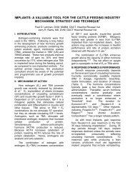
Industrial and Environmental Applications<br />
<strong>HYDRUS</strong> models - Governing Equations<br />
Source Zone<br />
Observation wells<br />
Control Planes<br />
Variably-Saturated Water Flow (Richards Equation)<br />
∂θ<br />
∂ ∂h<br />
= [ Kh ( ) −Kh ( )] −S<br />
∂t ∂z ∂z<br />
Heat Movement<br />
∂Cp( θ ) T ∂ ∂T ∂qT<br />
= [ λθ ( ) ] −Cw<br />
−CwST<br />
∂t ∂z ∂z ∂z<br />
Solute Transport<br />
∂( ρs) ∂( θ c)<br />
∂ ∂c<br />
+ = ( θD<br />
−qc)<br />
−φ<br />
∂t ∂t ∂z ∂z<br />
The <strong>HYDRUS</strong> Software Packages<br />
Variably-Saturated Flow (Richards Eq.)<br />
Root Water Uptake (water, salinity stress)<br />
Multiple Solutes (decay chains, ADE)<br />
Nonlinear Sorption<br />
Two-Site Nonequilibrium Sorption<br />
Mobile-Immobile Water<br />
Heat Transport<br />
Pedotransfer Functions (hydraulic properties)<br />
Parameter Estimation<br />
Interactive Graphics-Based Interface<br />
<strong>HYDRUS</strong> - References<br />
Šimunek, J., M. Šejna, and M. Th. van Genuchten, The <strong>HYDRUS</strong>-1D<br />
software package for simulating one-dimensional movement of water, heat,<br />
and multiple solutes in variably saturated media. Version 2.0, IGWMC - TPS<br />
- 70, International Ground Water Modeling Center, Colorado School of<br />
Mines, Golden, Colorado, 202pp., 1998.<br />
Šimunek, J., M. Šejna, and M. Th. van Genuchten, The <strong>HYDRUS</strong>-2D<br />
software package for simulating two-dimensional movement of water, heat,<br />
and multiple solutes in variably saturated media. Version 2.0, IGWMC - TPS<br />
- 53, International Ground Water Modeling Center, Colorado School of<br />
Mines, Golden, Colorado, 251pp., 1999.<br />
E-mail: igwmc@mines.edu<br />
http://www.mines.edu/igwmc<br />
http://www.ussl.ars.usda.gov/models/hydrus2d.HTM<br />
http://www.pc-progress.cz
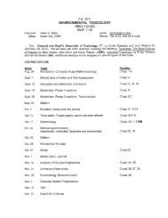
<strong>HYDRUS</strong>-2D - History of Development<br />
Israel: Neuman [1972] - UNSAT<br />
U. of Arizona: Davis and Neuman [1983]<br />
Agr. U. in Wageningen:<br />
Feddes et al. [1978]<br />
Vogel [1987] - SWMII<br />
USSL - SWMS-2D<br />
Šimunek et al. [1992]<br />
USSL - <strong>HYDRUS</strong>-2D (1.0)<br />
Šimunek et al. [1996]<br />
Princeton U.:<br />
van Genuchten [1978]<br />
MIT:<br />
Celia et al. [1990]<br />
USSL - CHAIN-2D<br />
Šimunek et al. [1994]<br />
USSL - <strong>HYDRUS</strong>-2D (2.0)<br />
Šimunek et al. [1999]<br />
<strong>HYDRUS</strong>-2D - History (References)<br />
Neuman, S. P., Finite element computer programs for flow in saturated-unsaturated<br />
porous media, Second Annual Report, Part 3, Project No. A10-SWC-77, 87 p.<br />
Hydraulic Engineering Lab., Technion, Haifa, Israel, 1972.<br />
Davis, L. A., and S. P. Neuman, Documentation and user's guide: UNSAT2 -Variably<br />
saturated flow model, Final Report, WWL/TM-1791-1, Water, Waste & Land, Inc., Ft.<br />
Collins, Colorado, 1983.<br />
van Genuchten, Mass transport in saturated-unsaturated media: One-dimensional<br />
solution, Research Rep. No. 78-WR-11, Water Resources Program, Princeton Univ.,<br />
Princeton, NJ, 1978.<br />
Celia, M. A., and E. T. Bouloutas, R. L. Zarba, A general mass-conservative numerical<br />
solution for the unsaturated flow equation, Water Resour. Res., 26(7), 1483-1496, 1990.<br />
Vogel, T. SWMII - Numerical model of two-dimensional flow in a variably saturated<br />
porous medium, Research Report No. 87, Dept. of Hydraulics and Catchment<br />
Hydrology, Agricultural Univ., Wageningen, The Netherlands, 1987.<br />
Šimunek, J., T. Vogel, and M. Th. van Genuchten. The SWMS_2D code for simulating<br />
water flow and solute transport in two-dimensional variably saturated media, Version<br />
1.1. Research Report No. 126, 169 p., U.S. Salinity Laboratory, USDA, ARS,<br />
Riverside, California, 1992.<br />
<strong>HYDRUS</strong> –Modular Structure<br />
<strong>HYDRUS</strong> Graphical Interface<br />
Input, Output, Meshgen<br />
Water Flow<br />
Solute Transport<br />
Heat Transport<br />
<strong>HYDRUS</strong> – Main Module<br />
Soil Hydraulic Properties<br />
Pedotransfer Functions<br />
Root Uptake<br />
Equation Solvers<br />
Inverse Optimization<br />
The <strong>HYDRUS</strong> Software Packages<br />
Variably-Saturated Flow (Richards Eq.)<br />
Root Water Uptake (water, salinity stress)<br />
Multiple Solutes (decay chains, ADE)<br />
Nonlinear Sorption<br />
Two-Site Nonequilibrium Sorption<br />
Mobile-Immobile Water<br />
Heat Transport<br />
Pedotransfer Functions (hydraulic properties)<br />
Parameter Estimation<br />
Interactive Graphics-Based Interface<br />
Water Flow - Richards’ Equation<br />
The governing flow equation for two-dimensional isothermal<br />
Darcian flow in a variably saturated isotropic rigid porous medium:<br />
∂ θ ∂<br />
=<br />
∂ t ∂ x<br />
i<br />
⎡<br />
⎢ K ( K<br />
⎢⎣<br />
A<br />
ij<br />
∂ h<br />
∂ x<br />
j<br />
+ K<br />
A<br />
iz<br />
θ - volumetric water content [L 3 L -3 ]<br />
h - pressure head [L]<br />
K - unsaturated hydraulic conductivity [LT -1 ]<br />
K ijA - components of a anisotropy tensor [-]<br />
x i - spatial coordinates [L]<br />
z - vertical coordinate positive upward [L]<br />
t - time [T]<br />
S - root water uptake [T -1 ]<br />
⎤<br />
) ⎥ − S<br />
⎥⎦<br />
Richards Equation - Assumptions<br />
Effect of air phase is neglected<br />
Darcy’s equation is valid at very low and very high<br />
velocities<br />
Osmotic gradients in the soil water potential are negligible<br />
Fluid density is independent of solute concentration<br />
Matrix and fluid compressibilities are relatively small
Soil Hydraulic Properties<br />
Retention Curve, θ(h)<br />
(Soil-water characteristic curve)<br />
- characterizes the energy status of the soil water<br />
|Pressure head| [cm]<br />
500<br />
400<br />
300<br />
200<br />
100<br />
0<br />
Loam<br />
Sand<br />
Clay<br />
0 0.1 0.2 0.3 0.4 0.5<br />
Water Content [-]<br />
Soil Hydraulic Properties<br />
Hydraulic Conductivity Function, K(h)<br />
- resistance of porous media to water flow<br />
log (Hydraulic Conductivity [cm/d])<br />
4<br />
2<br />
0<br />
-2<br />
-4<br />
-6<br />
-8<br />
-10<br />
0 1 2 3 4 5<br />
log (|Pressure Head| [cm])<br />
Loam<br />
Sand<br />
Clay<br />
Soil Hydraulic Properties<br />
Hydraulic Conductivity Function, K(θ)<br />
log (Hydraulic Conductivity [cm/d])<br />
4<br />
2<br />
0<br />
-2<br />
-4<br />
-6<br />
Loam<br />
Sand<br />
-8<br />
Clay<br />
-10<br />
0 0.1 0.2 0.3 0.4 0.5<br />
Water Content [-]<br />
Retention Curve<br />
Brooks and Corey [1964]:<br />
van Genuchten [1980]:<br />
Kosugi [1996]:<br />
θ s - saturated water content [-]<br />
θ r - residual water content [-]<br />
α, n, h 0 , σ - empirical parameters [L -1 ], [-], [L], [-]<br />
S e - effective water content [-]<br />
-n<br />
⎧ | α h|<br />
h < -1/ α<br />
S e = ⎨<br />
⎩ 1 h ≥ -1/ α<br />
S 1<br />
= e 1 1/<br />
(1 α h<br />
n −<br />
+ )<br />
n<br />
( h h0<br />
)<br />
σ<br />
1 ⎧ln / ⎫<br />
Se<br />
= erfc⎨ ⎬<br />
2 ⎩ 2 ⎭<br />
θ −θr<br />
Se<br />
=<br />
θ −θ<br />
s<br />
r<br />
Hydraulic Conductivity Function<br />
Brooks and Corey [1964]:<br />
Kh ( ) = K s S<br />
2/ n + l + 2<br />
e<br />
Soil Water Retention Curve, 2(h)<br />
van Genuchten [1980]:<br />
(Mualem [1976])<br />
1/ m<br />
( )<br />
l<br />
K( h) = K S ⎡ 1− 1−<br />
S<br />
⎢⎣<br />
S e e<br />
m<br />
⎤<br />
⎥⎦<br />
2<br />
Kosugi [1996]:<br />
(Mualem [1976])<br />
θ s - saturated water content [-]<br />
θ r - residual water content [-]<br />
α, n, h 0 , σ, l - empirical parameters [L -1 ], [-], [L], [-], [-]<br />
S e - effective water content [-]<br />
Κ S - saturated hydraulic conductivity [LT -1 ]<br />
( h h0<br />
)<br />
σ<br />
⎧<br />
l ⎪1<br />
⎡ln / ⎤⎫⎪<br />
Kh ( ) = KS<br />
s e⎨<br />
erfc⎢<br />
+ σ ⎥⎬<br />
⎪⎩2 ⎣ 2 ⎦⎪⎭<br />
θ −θr<br />
Se<br />
=<br />
θ −θ<br />
s<br />
r<br />
2
Hydraulic Conductivity Function, K(2)<br />
Richards Equation - Complications<br />
Hysteresis in the soil water retention function<br />
Extreme nonlinearity of the hydraulic functions<br />
Lack of accurate and cheap methods for measuring<br />
the hydraulic properties<br />
Extreme heterogeneity of the subsurface<br />
Inconsistencies between scale at which the<br />
hydraulic and solute transport parameters are<br />
measured, and the scale at which the models are<br />
being applied<br />
Soil Water Hysteresis<br />
Boundary Conditions: System-Independent<br />
Pressure head (Dirichlet type) boundary conditions:<br />
h(<br />
x, z, t)<br />
= ψ ( x, z, t)<br />
for ( x, z)<br />
ε<br />
Flux (Neumann type) boundary conditions:<br />
Γ D<br />
∂h<br />
- [ K ( K + K )] n = σ ( x, z, t) for ( x, z)<br />
ε Γ<br />
∂x<br />
j<br />
A<br />
A<br />
ij iz i 1<br />
N<br />
Gradient boundary conditions:<br />
A ∂h<br />
A<br />
( K ij + K iz ) n i = σ 2 ( x,<br />
z,<br />
t)<br />
for ( x,<br />
z)<br />
ε Γ<br />
∂ x j<br />
G<br />
Boundary Conditions: System-Dependent<br />
Atmospheric boundary condition:<br />
∂h<br />
| -K -K| ≤ E hA≤h<br />
≤hS<br />
∂x<br />
Ponding<br />
0<br />
-20<br />
-20<br />
-25<br />
-30<br />
-40<br />
-35<br />
Boundary Conditions: System-Dependent<br />
Seepage face (free draining lysimeter, dike)<br />
if(h q=0<br />
if(h=0) => q=<br />
Tile drains<br />
1D soil profile<br />
Soil surface<br />
Groundwater table<br />
-60<br />
-80<br />
-100<br />
0 0.025 0.05 0.075 0.1<br />
Time [days]<br />
-40<br />
-45<br />
-50<br />
-55<br />
0.00 0.05 0.10 0.15 0.20<br />
Time [days]<br />
Tile drain<br />
Impermeable layer
The <strong>HYDRUS</strong> Software Packages<br />
Variably-Saturated Flow (Richards Eq.)<br />
Root Water Uptake (water, salinity stress)<br />
Multiple Solutes (decay chains, ADE)<br />
Nonlinear Sorption<br />
Two-Site Nonequilibrium Sorption<br />
Mobile-Immobile Water<br />
Heat Transport<br />
Pedotransfer Functions (hydraulic properties)<br />
Parameter Estimation<br />
Interactive Graphics-Based Interface<br />
Root Water Uptake<br />
Bresler et al. [1982]<br />
S( z,t ) = - b ( z) K( )[ h -h( z,t) ]<br />
1 θ<br />
Feddes et al. [1978]<br />
S( z,t ) = - b 2( z) α 1( h( z,t )) T p<br />
r<br />
1<br />
van Genuchten (1987):<br />
Y / Ym<br />
1 ( c/ c50)<br />
= + p<br />
The <strong>HYDRUS</strong> Software Packages<br />
Variably-Saturated Flow (Richards Eq.)<br />
Root Water Uptake (water, salinity stress)<br />
Multiple Solutes (decay chains, ADE)<br />
Nonlinear Sorption<br />
Two-Site Nonequilibrium Sorption<br />
Mobile-Immobile Water<br />
Heat Transport<br />
Pedotransfer Functions (hydraulic properties)<br />
Parameter Estimation<br />
Interactive Graphics-Based Interface<br />
General structure of the system of solutes:<br />
Products<br />
Products<br />
µ g,1 µ w,1 µ s,1 µ g,2 µ w,2 µ s,2<br />
A µ w,1 B µ w,2 C ...<br />
g 1 c 1 s 1 µ s,1 g 2 c 2 s 2 µ s,2<br />
k g,1 k s,1<br />
µ g,1<br />
k g,2 k s,2<br />
µ g,2<br />
γ g,1 γ w,1 γ s,1 γ g,2 γ w,2 γ s,2<br />
Products<br />
Products<br />
Typical examples of sequential<br />
first-order chains:<br />
Radionuclides [van Genuchten, 1985]<br />
238<br />
Pu<br />
234<br />
U<br />
230<br />
Th<br />
226<br />
Ra<br />
c 1 s 1 c 2 s 2 c 3 s 3 c 4 s 4<br />
Nitrogen [Tillotson et al., 1980]<br />
g2 N 2<br />
(NH 2 ) 2 CO NH<br />
+ 4 NO<br />
- 2 NO<br />
- 3<br />
c 1 s 1 c 2 s 2 c 3 c 4 N 2 O
Typical examples of sequential firstorder<br />
chains: Pesticides [Wagenet and Hutson, 1987]<br />
Uninterrupted chain - one reaction path:<br />
Gas<br />
Parent Daughter Daughter<br />
pesticide product 1 product 2 Products<br />
c 1 s 1 c 2 s 2 c 3 s 3<br />
Product Product Product<br />
(aldicarb, oxime) (sulfone, sulfone oxime) (sulfoxide, sulfoxide oxime)<br />
Interrupted chain - two independent reaction paths:<br />
Gas<br />
Gas<br />
Typical examples of sequential firstorder<br />
chains: Organic Hydrocarbons<br />
Dechlorination of chlorinated ethenes<br />
[Schaerlaekens et al., 1999; Casey and Simunek, 2002]<br />
t-DCE<br />
PCE TCE c-DCE VC ethylene<br />
1,2-DCE<br />
Parent Daughter Parent<br />
pesticide 1 product 1 Products pesticide 2 Products<br />
c 1 s 1 c 2 s 2 c 3 s 3 c 4 s 4<br />
Product Product Product<br />
Perchloroethylene<br />
trichloroethylene dichloroethylene vinylchloride<br />
Typical Examples of Sequential Firstorder<br />
Chains: Pharmaceuticals and Explosives<br />
Pharmaceuticals, hormones (Estrogen, Testosterone):<br />
Estradiol Estrone Estriol<br />
Explosives (TNT, RDX HMX)<br />
4ADNT<br />
TNT<br />
2ADNT<br />
4ADNT<br />
4ADNT<br />
TAT<br />
2,4,6 trinitrotoluene 2-amino-4,6-dinitrotoluene 4-amino-2,6-dinitrotoluene 2,4,6-triminotoulene<br />
Governing Solute Transport Equations<br />
∂θc ∂ρs ∂ag ∂ ∂c<br />
∂ ∂g ∂qc<br />
+ + = ( θ ) + ( a )- -<br />
∂ ∂ ∂ ∂ ∂ ∂ ∂ ∂<br />
-( µ + µ ) -( µ + µ ) -( µ + µ ) a + +<br />
−µ<br />
(2, )<br />
k k k w k g k i k<br />
Dij,k<br />
Dij,k<br />
t t t xi x j xi x j xi<br />
' ' ' '<br />
θ<br />
w,k w,k ck ρ<br />
s,k s,k sk g,k g,k<br />
g µ<br />
k w,k −1θck-1<br />
'<br />
'<br />
s,k −1<br />
ρ sk −1 -µ g,k −1 a g<br />
k−1+ γ<br />
w,kθ+ γ<br />
s,kρ+ γ<br />
g,ka−Scr , k<br />
kε<br />
ns<br />
w, s, g subscripts corresponding with the liquid, solid and gaseous phases,<br />
respectively<br />
c, s, g concentration in liquid, solid, and gaseous phase, respectively<br />
2,4DANT; 2,6DANT; 2,4DNT; 2,6DNT<br />
Governing Solute Transport Equations<br />
q i i-th component of the volumetric flux<br />
ρ soil bulk density<br />
a air content<br />
S sink term in the water flow equation<br />
c r concentration of the sink term<br />
D ijw ,D<br />
g<br />
ij dispersion coefficient tensor for the liquid and gaseous phase, respectively<br />
k subscript representing the kth chain number<br />
µ w , µ s , µ g first-order rate constants for solutes in the liquid, solid, and gaseous phases,<br />
respectively<br />
γ w , γ s , γ g zero-order rate constants for the liquid, solid, and gaseous phases,<br />
respectively<br />
µ w ', µ s ', µ g ' first-order rate constants for solutes in the liquid, solid and gaseous phases,<br />
respectively; these rate constants provide connections between the individual<br />
chain species.<br />
number of solutes involved in the chain reaction<br />
n s<br />
The <strong>HYDRUS</strong> Software Packages<br />
Variably-Saturated Flow (Richards Eq.)<br />
Root Water Uptake (water, salinity stress)<br />
Multiple Solutes (decay chains, ADE)<br />
Nonlinear Sorption<br />
Two-Site Nonequilibrium Sorption<br />
Mobile-Immobile Water<br />
Heat Transport<br />
Pedotransfer Functions (hydraulic properties)<br />
Parameter Estimation<br />
Interactive Graphics-Based Interface
3<br />
3<br />
Interactions Among Phases<br />
Linear Adsorption<br />
s =<br />
∂ Rθ<br />
c<br />
∂ t<br />
Steady-State<br />
∂<br />
R<br />
c ∂ t<br />
kc<br />
∂<br />
⎛<br />
∂<br />
⎞<br />
⎜ c<br />
= θ<br />
⎟<br />
+ φ<br />
∂ ⎜<br />
D − q c<br />
x<br />
ij<br />
∂ x<br />
i ⎟<br />
i ⎝<br />
j ⎠<br />
2<br />
∂ c ∂ c<br />
= D − v<br />
2<br />
∂ z ∂ z<br />
Nonlinear Equilibrium Adsorption<br />
+ k c<br />
Equation Model Reference<br />
s=kc+k 1<br />
Linear Lapidus and Amundson [1952]<br />
2<br />
Lindstrom et al. [1967]<br />
s=k 1 c k 2 Freundlich Freundlich [1909]<br />
k c<br />
Langmuir Langmuir [1918]<br />
1<br />
s =<br />
1 + k c 2<br />
k<br />
k c<br />
Freundlich-Langmuir Sips [1950]<br />
1<br />
s =<br />
1<br />
k + k 2 c<br />
k 1 c<br />
1 1 + k 4 c<br />
k 3 c<br />
Double Langmuir Shapiro and Fried [1959]<br />
s=<br />
2<br />
c<br />
s=k c k<br />
1<br />
2 / k 3 Extended Freundlich Sibbesen [1981]<br />
k c<br />
Gunary Gunary [191970]<br />
1<br />
s =<br />
1 + k 2 c + k 3 c<br />
k 2<br />
s=kc 1 - k<br />
Fitter-Sutton Fitter and Sutton [1975]<br />
3<br />
s=k - + k c k 3<br />
1 1 k 4<br />
{ [ ] } Barry Barry [1992]<br />
1 2<br />
2<br />
RT ln( ) Temkin Bache and Williams [1971]<br />
s =<br />
k c<br />
k 1<br />
s=k 1cexp( -2<br />
k 2s) Lindstrom et al. [1971]<br />
van Genuchten et al. [1974]<br />
s<br />
=<br />
c<br />
modified Kielland Lai and Jurinak [1971]<br />
sT [ c+ k1( cT −c)exp{ k2( cT−2c)}]<br />
Interactions Among Phases<br />
Equilibrium interactions between the solution (c)<br />
and gaseous (g) concentrations (Henry’s law)<br />
Nonequilibrium interactions between the solution<br />
(c) and adsorbed (s) concentrations<br />
A generalized nonlinear empirical equation<br />
β<br />
kc<br />
d<br />
s=<br />
1 + c<br />
β<br />
η<br />
k d , η , β<br />
empirical constants<br />
The <strong>HYDRUS</strong> Software Packages<br />
Variably-Saturated Flow (Richards Eq.)<br />
Root Water Uptake (water, salinity stress)<br />
Multiple Solutes (decay chains, ADE)<br />
Nonlinear Sorption<br />
Two-Site Nonequilibrium Sorption<br />
Mobile-Immobile Water<br />
Heat Transport<br />
Pedotransfer Functions (hydraulic properties)<br />
Parameter Estimation<br />
Interactive Graphics-Based Interface<br />
Non-Equilibrium Adsorption Equations<br />
Nonequilibrium two-site adsorption model<br />
[1952]<br />
Equation Model Reference<br />
∂s<br />
∂t Linear Lapidus and Amundson<br />
1 2<br />
Oddson et al. [1970]<br />
∂ s<br />
k 2<br />
= α ( kc -s)<br />
Freundlich Hornsby and Davidson [1973]<br />
1<br />
∂ t van Genuchten et al. [1974]<br />
∂s<br />
⎛ ⎞<br />
⎜<br />
k1c<br />
= α - s⎟<br />
∂t<br />
⎝1+k<br />
2c<br />
⎠<br />
Langmuir Hendricks [1972]<br />
∂s<br />
⎛ k3<br />
⎞<br />
⎜<br />
k1c<br />
= α - s<br />
⎟<br />
Freundlich- Šimunek and van Genuchten [1994]<br />
∂t<br />
k3<br />
⎝1+k<br />
2c<br />
⎠<br />
Langmuir<br />
∂s<br />
⎛ s - s ⎞<br />
⎜ T ⎟<br />
Fava and Eyring [42]<br />
= α ( s -s)sinh<br />
T ∂<br />
⎜<br />
k1<br />
t<br />
s - ⎟<br />
⎝ T si<br />
⎠<br />
∂s<br />
∂t α exp( k s ){ k c exp( -2 k s ) -s }<br />
Lindstrom et al. [1971]<br />
∂s<br />
∂t = c k<br />
s k<br />
α Leenheer and Ahlrichs [1971]<br />
1 2<br />
Enfield et al. [1976]<br />
s<br />
e k<br />
s<br />
k k<br />
f<br />
s k= s e k+ sk k<br />
Type - 1 sites with instantaneous sorption<br />
Type - 2 sites with kinetic sorption<br />
e<br />
∂ sk<br />
∂ sk<br />
= f<br />
∂t<br />
∂t<br />
k<br />
β<br />
∂s<br />
⎡<br />
k<br />
k<br />
ks,k<br />
c ⎤<br />
k k k<br />
= αk<br />
⎢( 1-<br />
f<br />
k)<br />
- µ γ<br />
β<br />
sk⎥ -<br />
s,k sk<br />
+ (1 - f )<br />
∂t<br />
1+<br />
η<br />
k<br />
⎣<br />
kck<br />
⎦<br />
fraction of exchange sites assumed to be at equilibrium<br />
s,k
The <strong>HYDRUS</strong> Software Packages<br />
Variably-Saturated Flow (Richards Eq.)<br />
Root Water Uptake (water, salinity stress)<br />
Multiple Solutes (decay chains, ADE)<br />
Nonlinear Sorption<br />
Two-Site Nonequilibrium Sorption<br />
Mobile-Immobile Water<br />
Heat Transport<br />
Pedotransfer Functions (hydraulic properties)<br />
Parameter Estimation<br />
Interactive Graphics-Based Interface<br />
Two-Region Physical Nonequilibrium Transport<br />
∂<br />
∂ ∂<br />
+f k c = D c m<br />
( θ m ρ D) m ( θ m m -qc )-α( c -c )-( θµ + fρ k µ ) c<br />
∂t<br />
∂ z ∂z m m im l,m D s,m m<br />
∂cim<br />
[ θ im + ( 1- f) ρkD] = α( c - c )-[ θ µ + ( 1- f) ρ k µ ] c<br />
∂t<br />
m im im l,im D s,im im<br />
Interaction among phases<br />
Liquid - Gas: a linear relation<br />
g = k gc<br />
k g,k empirical constant equal to (K H RT A ) -1<br />
K H<br />
R<br />
T A<br />
Henry's Law constant<br />
universal gas constant<br />
absolute temperature<br />
Volatilization<br />
∂( ρs) ∂( θc) ∂( ) ∂ ∂ ∂<br />
+ + ag = ( θD c ) φ<br />
∂t<br />
∂t<br />
∂t<br />
∂ x ∂x +aD g w<br />
a w a<br />
ij<br />
ij<br />
-qi<br />
c-qi<br />
g +<br />
∂x Steady-State:<br />
i<br />
g = kH<br />
c<br />
j<br />
i<br />
j<br />
j<br />
w<br />
i<br />
⎛ ρ k ak ⎞<br />
2 q q<br />
D H c w a a c +<br />
⎜<br />
∂ ⎛<br />
⎞ ∂<br />
1 + + ⎟ = ⎜D<br />
+ D k ⎟ -<br />
θ θ<br />
∂t<br />
ij ij H<br />
⎝<br />
⎠ ⎝ θ ⎠ ∂x<br />
∂x<br />
θ<br />
a<br />
k<br />
i H<br />
∂c<br />
∂x<br />
i<br />
Temperature Dependence of Transport<br />
and Reaction Coefficients<br />
Most of the diffusion (D w , D g ), distribution (k s , k g ), and reaction<br />
rate (γ w , γ s , γ g , µ w ', µ s ', µ g ', µ w , µ s , and µ g ) coefficients are<br />
strongly temperature dependent. <strong>HYDRUS</strong>_2D assumes that<br />
this dependency can be expressed by an Arrhenius equation<br />
[Stumm and Morgan, 1981].<br />
A A<br />
⎡ E(<br />
T - T r ) ⎤<br />
aT<br />
= ar<br />
exp⎢<br />
A A ⎥<br />
⎣ RT T r ⎦<br />
a r ,a T coefficient values at a reference absolute temperature,<br />
T rA , and absolute temperature, T A , respectively<br />
E activation energy of the reaction or process<br />
Solute Transport - Dispersion Coefficient<br />
Bear [1972]:<br />
q<br />
j<br />
q<br />
θ D ij = D<br />
T<br />
| q | δ ij + ( D<br />
L<br />
- D<br />
T<br />
)<br />
| q |<br />
i<br />
+ θ D<br />
D d - ionic or molecular diffusion coefficient in free water [L 2 T -1 ]<br />
τ - tortuosity factor [-]<br />
δ ij - Kronecker delta function (δ ij =1 if i=j, and δ ij =0 otherwise)<br />
D L , D T - longitudinal and transverse dispersivities [L]<br />
2<br />
2<br />
q<br />
x<br />
q<br />
z<br />
θ D xx = D L + DT<br />
+ θ Dd<br />
τ<br />
| q | | q |<br />
2<br />
2<br />
q<br />
z<br />
q<br />
x<br />
θ D zz = D L + DT<br />
+ θ Dd<br />
τ<br />
| q | | q |<br />
q<br />
x<br />
q<br />
z<br />
θ D xz = ( D L - DT)<br />
| q |<br />
d<br />
τ δ<br />
ij
Solute Transport - Boundary Conditions<br />
First-type (or Dirichlet type) boundary conditions<br />
c( x, z, t ) = c 0( x, z, t ) for( x, z ) ε Γ D<br />
Third-type (Cauchy type) boundary conditions<br />
∂ c<br />
- θ Dij<br />
ni + qinic = qi0 nic0<br />
for ( x, z ) ε Γ<br />
∂ x j<br />
Second-type (Neumann type) boundary conditions<br />
∂ c<br />
θ Dij<br />
ni<br />
= 0 for ( x, z ) ε Γ<br />
∂ x j<br />
C<br />
N<br />
Dispersivity as a function of scale<br />
The <strong>HYDRUS</strong> Software Packages<br />
Variably-Saturated Flow (Richards Eq.)<br />
Root Water Uptake (water, salinity stress)<br />
Multiple Solutes (decay chains, ADE)<br />
Nonlinear Sorption<br />
Two-Site Nonequilibrium Sorption<br />
Mobile-Immobile Water<br />
Heat Transport<br />
Pedotransfer Functions (hydraulic properties)<br />
Parameter Estimation<br />
Interactive Graphics-Based Interface<br />
Governing Heat Transport Equation<br />
Sophocleous [1979]<br />
∂T<br />
C<br />
t = ∂ ∂T<br />
x x - ∂<br />
( θ) [ λ C q T ij( θ) ] w i<br />
∂ ∂ i ∂ j ∂ xi<br />
λ ij (θ) apparent thermal conductivity of the soil<br />
C(θ), C w volumetric heat capacities of the porous medium and the liquid phase,<br />
respectively<br />
de Vries [1963]<br />
C ( θ ) = C θ + C θ + C θ + C a<br />
n n o o w g<br />
θ volumetric fraction<br />
n, o, g, w subscripts representing solid phase, organic matter, gaseous phase, and<br />
liquid phase, respectively.<br />
Thermal Conductivity<br />
j i<br />
λ ij ( θ ) = λT C w |q| δ ij + ( λ L -λT ) C q q<br />
w + λ0( θ ) δ ij<br />
|q|<br />
λ 0 (θ) thermal conductivity of the porous medium (solid plus water)<br />
in the absence of flow<br />
λ L , λ T longitudinal and transverse thermal dispersivities,<br />
respectively<br />
Chung and Horton [1987]<br />
b 1 , b 2 , b 3<br />
( ) = b + b + b<br />
05 .<br />
λ 0 θ 1 2θ w 3θ<br />
w<br />
empirical parameters.<br />
The <strong>HYDRUS</strong> Software Packages<br />
Variably-Saturated Flow (Richards Eq.)<br />
Root Water Uptake (water, salinity stress)<br />
Multiple Solutes (decay chains, ADE)<br />
Nonlinear Sorption<br />
Two-Site Nonequilibrium Sorption<br />
Mobile-Immobile Water<br />
Heat Transport<br />
Pedotransfer Functions (hydraulic properties)<br />
Parameter Estimation<br />
Interactive Graphics-Based Interface
Pedotransfer Functions: Rosetta<br />
Schaap et al. (2001)<br />
Model<br />
Input Data<br />
TXT<br />
Textural Class<br />
SSC Sand, Silt, Clay %<br />
SSCBD<br />
Same + Bulk Density<br />
SSCBD + 2 33<br />
SSCBD + 2 at 33 kPa<br />
SSCBD + 2 33 + 2 1500 Same + 2 at 1500 kPa<br />
Estimation of Soil Hydraulic Properties With<br />
Artificial Neural Networks<br />
Log Suction [cm]<br />
4<br />
3<br />
2<br />
1<br />
0<br />
Sand<br />
Retention<br />
Clay<br />
0.2 0.4 0.6<br />
Water Content [cm 3 /cm 3 ]<br />
Sand Clay<br />
Sand % 79 28<br />
Silt % 13 29<br />
Clay % 8 43<br />
Bulk d. 1.45 1.44<br />
Probability<br />
Saturated Conductivity<br />
0.25<br />
0.2<br />
0.15<br />
Sand<br />
0.1 Clay<br />
0.05<br />
Log K(h) [cm/day]<br />
0<br />
Log(K s ) [cm/day ]<br />
Unsaturated Conductivity<br />
2<br />
0<br />
-2<br />
-4<br />
-6<br />
Clay<br />
1 2 3 4<br />
Sand<br />
1 2 3 4<br />
Log Suction [cm]<br />
The <strong>HYDRUS</strong> Software Packages<br />
Variably-Saturated Flow (Richards Eq.)<br />
Root Water Uptake (water, salinity stress)<br />
Multiple Solutes (decay chains, ADE)<br />
Nonlinear Sorption<br />
Two-Site Nonequilibrium Sorption<br />
Mobile-Immobile Water<br />
Heat Transport<br />
Pedotransfer Functions (hydraulic properties)<br />
Parameter Estimation<br />
Interactive Graphics-Based Interface<br />
Parameter Estimation in <strong>HYDRUS</strong><br />
Parameter Estimation:<br />
- Soil hydraulic parameters<br />
- Solute transport and reaction parameters<br />
- Heat transport parameters<br />
Sequence:<br />
- Independently<br />
- Simultaneously<br />
- Sequentially<br />
Method:<br />
- Marquardt-Levenberg optimization<br />
Objective Function<br />
Φ ( b , q , p ) =<br />
m q n q j<br />
*<br />
∑ v j ∑ w i, j [ q<br />
j<br />
j = 1 i = 1<br />
m p n p j<br />
*<br />
∑ v j ∑ w i, j<br />
[ p<br />
j<br />
j = 1 i = 1<br />
n b<br />
* 2<br />
∑ vˆ<br />
j [ b j - b j ]<br />
j = 1<br />
( x, t i)<br />
- q<br />
( θ ) -<br />
i<br />
( x, t i , b ) ] +<br />
p ( θ , b ) ] +<br />
1st term: deviations between measured and calculated space-time<br />
variables<br />
2nd term: differences between independently measured, p j* , and<br />
predicted , p j , soil hydraulic properties<br />
3rd term: penalty function for deviations between prior knowledge<br />
of the soil hydraulic parameters, b j* , and their final<br />
estimates, b j .<br />
j<br />
j<br />
i<br />
2<br />
2<br />
The <strong>HYDRUS</strong> Software Packages<br />
Variably-Saturated Flow (Richards Eq.)<br />
Root Water Uptake (water, salinity stress)<br />
Multiple Solutes (decay chains, ADE)<br />
Nonlinear Sorption<br />
Two-Site Nonequilibrium Sorption<br />
Mobile-Immobile Water<br />
Heat Transport<br />
Pedotransfer Functions (hydraulic properties)<br />
Parameter Estimation<br />
Interactive Graphics-Based Interface
Furrow Irrigation – Pressure Heads<br />
Dike – Pressure Heads<br />
Dike - Velocity Vectors<br />
Finite Element Mesh – Cut-off Wall<br />
Solute Plume Under Dam<br />
Capillary Barrier - Material Distributions
Capillary Barrier - Velocity Vectors<br />
Mesh Generator<br />
Tunnel - Spectral Color Maps<br />
Tunnel - Velocity Vectors<br />
Plume Movement in a Transect with Stream<br />
<strong>HYDRUS</strong> - Existing Applications<br />
Agricultural:<br />
Irrigation management (FREP, LINK , Bristow et al., 2002)<br />
Drip irrigation design (FREP, LINK, Bristow et al., 2002)<br />
Sprinkler irrigation design (FREP, LINK)<br />
Tile drainage design and performance (Mohanty et al., 1998, do Vos et al., 2000)<br />
Studies of root and crop growth (Vrugt et al., 2001, 2002)<br />
Salinization and reclamation processes (Šimůnek and Suarez, 1998)<br />
Nitrogen dynamics and leaching (Ventrella et al., 2001; Jacques et al., 2002)<br />
Transport of pesticides and degradation products (Wang et al., 1998)<br />
Non-point source pollution<br />
Seasonal simulation of water flow and plant response<br />
. . .
<strong>HYDRUS</strong> - Existing Applications<br />
Non-Agricultural:<br />
Leaching from radioactive waste sites at the Nevada test Site (DRI, DOE)<br />
Flow around nuclear subsidence craters at the Nevada test site (Pohll et al., 1996;<br />
Wilson et al., 2000)<br />
Capillary barrier at Texas low-level radioactive waste disposal site (Scanlon, 1998)<br />
Evaluation of approximate analytical analysis of capillary barriers (Morris and<br />
Stormont, 1997; Kampf and Montenegro, 1997; Heiberger, 1998)<br />
Landfill covers with and without vegetation (Abbaspour et al, 1997; Albright, 1997; Gee et al.,<br />
1999, Scanlon et al., 2002)<br />
Risk analysis of contaminant plumes from landfills<br />
Seepage of wastewater from land treatment systems<br />
Tunnel design - flow around buried objects (Knight, 1999)<br />
Highway design - road construction - seepage (de Haan, 2002)<br />
Stochastic analyses of solute transport in heterogeneous media (Tseng and Jury, 1993;<br />
Roth, 1995; Roth and Hammel, 1996; Kasteel et al. 1999; Hammel et al., 1999; Roth et al., 1999; Vanderborght et<br />
al., 1998, 1999)<br />
Lake basin recharge analysis (Lee, 2000)<br />
<strong>HYDRUS</strong> - Existing Applications<br />
Non-Agricultural:<br />
Stream-aquifer interactions<br />
Environmental impact of the drawdown of shallow water tables<br />
Analysis of cone permeameter and tension infiltrometer experiments (Gribb et al.,<br />
1996; Kodesova et al., 1998, 1999; Šimůnek et al., 1997, 1998, 1999)<br />
Virus and bacteria transport (Shijven and Šimůnek, 2002, Bradford et al., 2002a,b, Yates et al., 2000)<br />
Hill-slope analyses<br />
Transport of TCE and its degradation products (Scharlaekens et al., 2000; Casey and<br />
Simunek, 2002)<br />
Multicomponent geochemical transport (Jacques and Šimůnek, 2002)<br />
Analyses of riparian systems (Whitaker, 2000)<br />
Fluid flow and chemical migration within the capillary fringe (Silliman et al., 2002)<br />
Flow in historical monuments (Ishizaki et al., 2001)<br />
Flow and transport around land mines (Das et al., 2001; Šimůnek et al., 2001)<br />
Analyses of Chloride profiles in deep vadose zones to evaluate historical fluxes<br />
(Scanlon et al., 2003)<br />
Current and Future Development<br />
Coupled movement of water and energy,<br />
including vapor transport<br />
Modified Richards Equation:<br />
∂θ<br />
∂ ⎡ ∂<br />
Lh<br />
( ) ∂<br />
K h K<br />
Lh<br />
( h) K<br />
LT<br />
( h)<br />
T ∂<br />
K h ∂ T ⎤<br />
= + + +<br />
vh<br />
+ KvT<br />
− S<br />
∂t ∂z ⎢<br />
⎣ ∂z ∂z ∂z ∂z<br />
⎥<br />
⎦<br />
K Lh - hydraulic conductivity for liquid phase fluxes due to gradient in h<br />
K LT - hydraulic conductivity for liquid phase fluxes due to gradient in T<br />
K vh - isothermal vapor hydraulic conductivity<br />
K vT - thermal vapor hydraulic conductivity<br />
Energy Transport:<br />
∂ C T p ∂<br />
v<br />
T<br />
l v v<br />
L ∂ ⎡ ∂ ⎤ ∂<br />
0<br />
λ( θ ) C qT ∂ q ∂<br />
+ = − qT<br />
w<br />
−CwST − L0<br />
−Cv<br />
∂t ∂t ∂z ⎣<br />
⎢ ∂z ⎦<br />
⎥ ∂z ∂z ∂z<br />
(1) (2) (3) (4) (5)<br />
(1) Soil heat flow by conduction<br />
(2) Convection of sensible heat by water flow<br />
(3) Heat removed by root water uptake<br />
(4) Transfer of latent heat by diffusion of water vapor<br />
(5) Transfer of sensible heat by diffusion of water vapor<br />
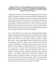
Coupled Movement of Water and Energy<br />
Coupled movement of water and energy<br />
-1000 -500 0<br />
0 1000 2000 3000 4000 5000<br />
0<br />
5<br />
0 yrs<br />
Central<br />
10 1 kyr<br />
5 kyr High Plains<br />
15 9 kyr<br />
Field<br />
20<br />
Amargosa Desert<br />
0<br />
10<br />
20<br />
0 yrs 10 kyr<br />
30<br />
5 kyr 16 kyr<br />
40 Field Lab<br />
50<br />
1 kyr<br />
5 kyr<br />
9 kyr<br />
Measured<br />
0 2000 4000 6000 8000 10000<br />
5 kyr<br />
10 kyr<br />
16 kyr<br />
Measured<br />
Depth [cm]<br />
10<br />
8<br />
6<br />
4<br />
2<br />
T=0<br />
t=0.25 d<br />
t=1<br />
t=5<br />
t=25<br />
10<br />
8<br />
6<br />
4<br />
2<br />
10<br />
T=0<br />
t=0.25 d<br />
t=1 8<br />
t=5<br />
t=25<br />
6<br />
4<br />
2<br />
T=0<br />
t=0.25 d<br />
t=1<br />
t=5<br />
t=25<br />
10<br />
8<br />
6<br />
4<br />
2<br />
T=0<br />
t=0.25 d<br />
t=1<br />
t=5<br />
t=25<br />
0<br />
5<br />
10<br />
15<br />
20<br />
Eagle Flat<br />
0 yrs<br />
5 kyr<br />
12 kyr<br />
Field<br />
Field - OP<br />
0 2000 4000 6000 8000 10000<br />
5 kyr<br />
12 kyr<br />
Measured<br />
0<br />
0<br />
0<br />
0<br />
0 0.05 0.1 0.15 0.2 0 0.02 0.04 0.06 0 10 20 30 0 2 4 6 8 10<br />
Water Content [-]<br />
Total Flux [cm/d]<br />
Temperature [C]<br />
Concentration [-]<br />
Hueco Bolson<br />
0<br />
5<br />
10 0 yrs 10 kyr<br />
15<br />
5 kyr 13 kyr<br />
Field<br />
20<br />
0 5000 10000 15000 20000<br />
5 kyr<br />
10 kyr<br />
13 kyr<br />
Measured<br />
Simulated matric potentials and chloride<br />
concentrations from wet initial conditions<br />
(pluvial period) to different times of<br />
upward flow. (Scanlon et al. 2003)<br />
Total flux=water flux+vapor flux
Coupled movement of water and energy,<br />
freezing/thawing cycle<br />
Modified Richards Equation:<br />
∂θ<br />
ρi<br />
∂θi<br />
∂ ⎡ ∂h ∂T ∂h ∂T<br />
⎤<br />
+ = K<br />
Lh<br />
( h) + K<br />
Lh<br />
( h) + K<br />
LT<br />
( h)<br />
+ Kvh + KvT<br />
− S<br />
∂t ρ<br />
w<br />
∂t ∂z ⎢<br />
⎣ ∂z ∂z ∂z ∂z<br />
⎥<br />
⎦<br />
K Lh - hydraulic conductivity for liquid phase fluxes due to gradient in h<br />
K LT - hydraulic conductivity for liquid phase fluxes due to gradient in T<br />
K vh - isothermal vapor hydraulic conductivity<br />
- thermal vapor hydraulic conductivity<br />
K vT<br />
Energy Transport:<br />
∂C T p v i<br />
T<br />
l v v<br />
L θ<br />
0<br />
L<br />
f<br />
ρ<br />
∂ ⎡ ∂ ⎤<br />
+ −<br />
i<br />
= λ( θ ) −C ∂qT q qT<br />
w<br />
−CwST − L 0<br />
−C<br />
∂<br />
v<br />
∂t ∂t ∂t ∂z ⎢<br />
⎣ ∂z ⎥<br />
⎦ ∂z ∂z ∂z<br />
(6) (1) (2) (3) (4) (5)<br />
(1) Soil heat flow by conduction<br />
(2) Convection of sensible heat by water flow<br />
(3) Heat removed by root water uptake<br />
(4) Transfer of latent heat by diffusion of water vapor<br />
(5) Transfer of sensible heat by diffusion of water vapor<br />
(6) Freezing/thawing term<br />
Coupled Movement of Water and Energy,<br />
Freezing/thawing Cycle<br />
Apparent Capacity [Jm -3 K -1 ]<br />
Apparent Capacity [Jm -3 K -1 ]<br />
1.00E+12<br />
1.00E+11<br />
1.00E+10<br />
1.00E+09<br />
1.00E+08<br />
1.00E+07<br />
1.00E+06<br />
0.02<br />
1.00E+12<br />
1.00E+11<br />
1.00E+10<br />
1.00E+09<br />
1.00E+08<br />
1.00E+07<br />
1.00E+06<br />
0.50<br />
0.00<br />
0.00<br />
-0.02 -0.04 -0.06<br />
Temperature [ o C]<br />
-0.50 -1.00<br />
Temperature [ o C]<br />
-0.08<br />
Silty clay<br />
Loam<br />
Sand<br />
-1.50<br />
Silty clay<br />
Loam<br />
Sand<br />
-0.10<br />
-2.00<br />
Apparent heat capacity<br />
for different textures<br />
Coupled movement of water and energy<br />
Freezing/thawing cycle<br />
Silty Clay<br />
Depths (cm):<br />
0, 0.5. 1, 2, 3.5, 5, 10<br />
4<br />
2<br />
0<br />
-2<br />
0<br />
-20000<br />
-40000<br />
Heterogeneity,<br />
Layering<br />
-4<br />
-60000<br />
-6<br />
-0.5 0.0 0.5 1.0 1.5 2.0<br />
Time [days]<br />
-80000<br />
-0.5 0.0 0.5 1.0 1.5 2.0<br />
Time [d ays]<br />
0.36<br />
0.34<br />
0.32<br />
0.30<br />
0.28<br />
0.26<br />
0.24<br />
-0.5 0.0 0.5 1.0 1.5 2.0<br />
Time [days]<br />
1.5<br />
1.4<br />
1.3<br />
1.2<br />
1.1<br />
1.0<br />
0.9<br />
0.8<br />
0.7<br />
-0.5 0.0 0.5 1.0 1.5 2.0<br />
Time [d ays]<br />
Nonequilibrium and Preferential Flow and Transport<br />
Dual-porosity approach (Richards eq. for water, mobileimmobile<br />
concept for solute)<br />
Dual-porosity approach (mobile-immobile concept for both<br />
water and solute)<br />
Dual-permeability approach (two overlapping porous media, one<br />
for matrix flow, one for preferential flow) [Gerke and van<br />
Genuchten, 1993]<br />
Kinematic wave approach for flow in macropores [Jarvis, 1991]<br />
Simplified first-order approach [Ross and Smettem, 2000]<br />
∂ θ<br />
θe<br />
−θ<br />
= f( θθ ,<br />
e) =<br />
∂t<br />
τ<br />
Dual-porosity hydraulic property models [Durner, 1994]<br />
Design experiments that would provide parameters for above<br />
models
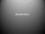
Dual-permeability Approach<br />
Gerke and van Genuchten [1993]: (two overlapping porous<br />
media, one for matrix flow, one for preferential flow)<br />
Flux [cm/d]<br />
60<br />
50<br />
40<br />
30<br />
20<br />
10<br />
0<br />
Fracture Flux<br />
Matrix Flux<br />
Mass Transfer<br />
Mass Transfer (-25%)<br />
Mass Transfer (+25%)<br />
0 0.02 0.04 0.06 0.08 0.1<br />
Time [d]<br />
Depth [cm]<br />
0<br />
5<br />
10<br />
15<br />
20<br />
t = 0.01 d<br />
25<br />
t = 0.04 d<br />
t = 0.08 d<br />
30<br />
t = 0.08 d (-25%)<br />
35<br />
t = 0.08 d (+25%)<br />
40<br />
0.25 0.3 0.35 0.4 0.45 0.5<br />
Water Content [-]<br />
Depth [cm]<br />
0<br />
5<br />
t = 0.01 d<br />
10<br />
t = 0.04 d<br />
t = 0.08 d<br />
15<br />
t = 0.08 d (-25%)<br />
t = 0.08 d (+25%)<br />
20<br />
25<br />
30<br />
35<br />
40<br />
0 0.005 0.01 0.015 0.02 0.025<br />
Water Content [-]<br />
Infiltration and mass exchange fluxes (a), water contents in the matrix<br />
(b) and fracture (c) domains<br />
Multicomponent solute transport:<br />
Coupling <strong>HYDRUS</strong> and PHREEQC [Parkhurst and<br />
Appelo, 1999])<br />
Available chemical reactions:<br />
Aqueous complexation<br />
Redox reactions<br />
Ion exchange (Gains-Thomas)<br />
Surface complexation – diffuse double-layer model and nonelectrostatic<br />
surface complexation model<br />
Precipitation/dissolution<br />
Chemical kinetics<br />
Biological reactions<br />
Verification of <strong>HYDRUS</strong>-PHREEQC<br />
Transport and Cation Exchange (major ions and heavy metals):<br />
(cations - Ca, Mg, Na, K, Cd, Pb, Zn; anions – Cl, Br, Al)<br />
a) Initially the 8-cm column contains a solution (with heavy metals) in equilibrium with the<br />
cation exchanger.<br />
b) The column is then flushed with three pore volumes of solution without heavy metals.<br />
Parameters:<br />
q=2 cm/d, λ=0.2 cm, CEC=11 mmol/cell.<br />
Initial concentrations: Al=0.5, Br=11.9, K=2, Na=6, Mg=0.75, Cd=0.09, Pb=0.1, Zn=0.25<br />
mmol/L.<br />
Boundary concentration: Al= 0.1, Br=3.7, Cl=10, Ca=5, Mg=1 mmol/L.<br />
Species and Complexes: Al 3+ , Al(OH) 2+ , Al(OH) 2+ , Al(OH) 3 , Al(OH) 4- , Br - ,Cl - , Ca 2+ ,<br />
Ca(OH) + , Cd 2+ , Cd(OH) + , Cd(OH) 2 , Cd(OH) 3- , Cd(OH) 2-<br />
4 , CdCl + ,<br />
CdCl 2 , CdCl 3- , K + , KOH, Na + ,NaOH, Mg 2+ , Mg(OH) + , Pb 2+ ,<br />
Pb(OH) + , Pb(OH) 2 , Pb(OH) 3- , Pb(OH) 2-<br />
4 ,PbCl + , PbCl 2 , PbCl 3- ,<br />
PbCl 2-<br />
4 , Zn 2+ , Zn(OH) + , Zn(OH) 2 , Zn(OH) 3- , Zn(OH) 2-<br />
4 , ZnCl + ,<br />
ZnCl 2 , ZnCl 3- , ZnCl 2<br />
4<br />
Exchange Species: AlX 3 , AlOHX 2 , CaX 2 , CdX 2 , KX, NaX, MgX 2 , PbX 2 , ZnX 2<br />
Verification of <strong>HYDRUS</strong>-PHREEQC<br />
Transport and cation<br />
exchange of major cations<br />
and heavy metals<br />
Concentration (mol/l)<br />
Concentration (mol/l)<br />
0.01<br />
0.008<br />
0.006<br />
0.004<br />
0.002<br />
0<br />
0.005<br />
0.004<br />
0.003<br />
0.002<br />
0.001<br />
0<br />
Na<br />
Al<br />
Cl<br />
Ca<br />
0 3 6 9 12 15<br />
Time (days)<br />
ZnX 2<br />
CdX 2<br />
CaX 2<br />
0 3 6 9 12 15<br />
Time (days)<br />
Concentration (mol/l)<br />
8E-004<br />
6E-004<br />
4E-004<br />
2E-004<br />
0E+000<br />
Relative mass balance errors (%)<br />
1.5<br />
1.2<br />
0.9<br />
0.6<br />
0.3<br />
0<br />
Pb<br />
Cd<br />
Zn<br />
0 3 6 9 12 15<br />
Time (days)<br />
Cl<br />
Ca<br />
Al<br />
Cd<br />
Zn<br />
0 3 6 9 12 15<br />
Time (days)<br />
Verification of <strong>HYDRUS</strong>-PHREEQC<br />
Kinetic biodegradation of NTA (nitrylotriacetate), cell growth,<br />
complexation with Co, and kinetic sorption<br />
Processes:<br />
Bacterially mediated degradation of an organic substrate<br />
Bacterial cell growth and death<br />
Aqueous speciation including metal-ligand complexation<br />
Kinetic sorption of Co and CoNTA<br />
Convective dispersive transport<br />
Parameters: L=10m, θ s =0.4 m, ρ=1.5 kg/m 3 , v=1 m/h, , λ=0.05 m.<br />
Iinitial Cond.: O 2 =3.125e-5, Na=0.001, Cl=0.001 mol/L, Biomass=0.000136g/L<br />
Boundary Cond.: O 2 =3.125e-5, Co=5.23e-6, NTA=5.23e-6, Na=0.001, Cl=0.001<br />
mol/L<br />
Verification of <strong>HYDRUS</strong>-PHREEQC<br />
Kinetic biodegradation of NTA, cell growth, complexation with Co, and kinetic sorption<br />
Rate equations:<br />
NTA degradation:<br />
RHNTA = −qm<br />
X<br />
2−<br />
[ HNTA ] [ O2<br />
]<br />
2−<br />
K<br />
s<br />
+ [ HNTA ] Ka<br />
+ [ O2<br />
]<br />
m<br />
2−<br />
Biomass production:<br />
R<br />
cell<br />
= −YR<br />
2 −<br />
HNTA<br />
Kinetic sorption (Co 2+ ,CoNTA - ):<br />
⎛ Z<br />
[ ] ⎟ ⎞<br />
R<br />
⎜<br />
Z<br />
= −k<br />
m<br />
Z −<br />
⎝ K<br />
d ⎠<br />
X m –biomass<br />
K s , K a – half-saturation constants<br />
Z – species concentration<br />
− bX<br />
m<br />
Concentrations [mol/g]<br />
1.6E-09<br />
1.2E-09<br />
8.0E-10<br />
4.0E-10<br />
0.0E+00<br />
Sorbed Co - PHREEQC<br />
Sorbed CoNta<br />
Sorbed Co - <strong>HYDRUS</strong><br />
Sorbed CoNta<br />
Biomass<br />
Biomass<br />
0 10 20 30 40 50 60 70 80<br />
Time [hours]<br />
4.0E-04<br />
3.0E-04<br />
2.0E-04<br />
1.0E-04<br />
0.0E+00<br />
Biomass [g/L]
Verification of <strong>HYDRUS</strong>-PHREEQC<br />
Kinetic biodegradation of NTA, cell growth, complexation with Co, and kinetic sorption<br />
Concentration [mol/kg]<br />
0.000004<br />
0.0000035<br />
0.000003<br />
0.0000025<br />
0.000002<br />
0.0000015<br />
0.000001<br />
0.0000005<br />
0<br />
CoNTA<br />
HNTA<br />
Co<br />
CoNTA<br />
HNTA<br />
Co<br />
pH<br />
pH<br />
0 10 20 30 40 50 60 70 80<br />
Time [hours]<br />
8<br />
7<br />
6<br />
5<br />
4<br />
3<br />
2<br />
1<br />
0<br />
Ph<br />
Constructed Wetlands<br />
12 Components:<br />
Dissolved oxygen O 2<br />
Organic matter: readily biodegradable, slowly biodegradable, inert<br />
Nitrogen: NH 4+ , NO 2- , NO 3- , N 2<br />
Inorganic phosphorus<br />
Heterotrophic micro-organisms<br />
Autotropic micro-organisms: Nitrosomonas & Nitrobacter<br />
9 Processes:<br />
Heterotrophic Organisms<br />
Hydrolysis<br />
Aerobic growth of heterotrophs on readily biodegradable OM<br />
NO 3 -growth of heterotrophs on readily biodegradable OM<br />
NO 2 -growth of heterotrophs on readily biodegradable OM<br />
Lysis<br />
Nitrosomonas<br />
Aerobic growth of N.somonas on NH 4<br />
Lysis of n-somonas<br />
Aerobic growth of N.bacter on NO 2<br />
Lysis of N.bacter<br />
Nitrobacter<br />
Overland Flow<br />
Kinematic wave equation:<br />
∂h ∂Q + = qxt ( , ) Q= αh<br />
∂t<br />
∂x<br />
h - unit storage of water (or mean depth),<br />
Q -discharge per unit width,<br />
q(x,t) - rate of local input, or lateral inflows (precipitation - infiltration)<br />
Manning hydraulic resistance law:<br />
1/2<br />
S<br />
α = 1.49 and m = 5/ 3<br />
n<br />
n - Manning’s roughness coefficient for overland flow<br />
S -slope<br />
m<br />
100*0.5 m<br />
<strong>HYDRUS</strong>-3D - Preview<br />
<strong>HYDRUS</strong>-3D - Preview<br />
<strong>HYDRUS</strong> Web Site – FAQ
<strong>HYDRUS</strong> Web Site – Tutorials<br />
<strong>HYDRUS</strong> Web Site – Discussion Forum<br />
<strong>HYDRUS</strong>-2D – User Manual<br />
David Rassam, Jirka Šimůnek and<br />
Rien Van Genuchten<br />
Introductory examples<br />
1. A Journey Through <strong>HYDRUS</strong> Windows<br />
1.1. Pre-Processing<br />
1.2. Post-Processing<br />
2. <strong>HYDRUS</strong> Output Files<br />
3. Root Water Uptake<br />
4. Example Application<br />
5. Inverse Solution<br />
6. Trouble Shooting<br />
Appendices:<br />
I. Soil Hydraulic Properties<br />
II. Concept Related to Modelling Evaporation<br />
III. Root Water Uptake<br />
IV. Scaling Factors<br />
V. Inverse Solution<br />
VI. Alphabetical Index for <strong>HYDRUS</strong> Windows