Flow Over a Cylinder - PhilonNet Engineering Solutions

Flow Over a Cylinder
Abstract—In this exercise, the flow over a cylinder is modeled. The cylinder is represented in two dimensions by
a circle, and a flow domain is created surrounding the circle. The diameter of the cylinder can be specified, and the
flow domain is adjusted based on these dimensions. Coarse, medium, and fine mesh types are available. Material
properties (density and viscosity), approach velocity, and physical models (inviscid and viscous) can be specified
within limits. Both steady and unsteady flow fields can be modeled. Static and total pressure, velocity at the outlet,
drag coefficient, and average shear stress are reported. Plots of pressure coefficient, pressure distribution, friction
coefficient, wall shear stress, and x-velocity distribution are available. Contours of static pressure, total pressure,
velocity, and stream function can be displayed. A velocity vector plot is also available.
1 Introduction
Flow over a cylinder is a fundamental fluid mechanics problem of practical importance. The flow field
over the cylinder is symmetric at low values of Reynolds number. As the Reynolds number increases, flow
begins to separate behind the cylinder causing vortex shedding which is an unsteady phenomenon. You can
apply either a steady state or an unsteady (time dependent) solver to capture these effects, as appropriate.
Drag forces acting on the walls of the cylinder are highly dependent upon Reynolds number. The effects of
viscosity and flow separation upon pressure distribution can be observed.
This exercise demonstrates that the drag coefficient and wall-shear stress depend upon the Reynolds number.
Additionally, the concept of dynamic similarity can be explored by comparing different combinations of
cylinder diameter and flow field velocity, while maintaining a constant Reynolds number.
Plots of pressure distribution and pressure coefficients along the surface of the cylinder demonstrate the
effects of flow separation on these parameters. It is also possible to animate the contour and vector plots
to visualize vortex shedding.
2 Modeling Details
The flow field around the cylinder is modeled in two dimensions with the axis of the cylinder perpendicular
to the direction of flow. The cylinder is modeled as a circle and a square flow domain is created around the
cylinder (Figure 2.1). A uniform velocity at the inlet of the flow domain can be specified. The procedure
for solving the problem is:
1. Create the geometry (cylinder and the flow domain).
2. Set the material properties and boundary conditions.
3. Mesh the domain.
FlowLab creates the geometry and mesh, and exports the mesh to FLUENT. The boundary conditions
and flow properties are set through parameterized case files. FLUENT converges the problem until the
convergence limit is met or the number of specified iterations is achieved.
1

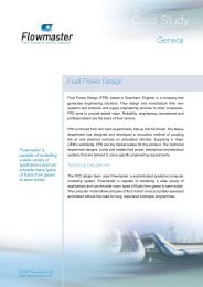
2.1 Geometry
Figure 2.1: Flow Domain
A flow domain is created surrounding the cylinder. The upstream length is 15 times the radius of the
cylinder, and the downstream length is 40 times the radius of the cylinder. The width of the flow domain is
50 times the radius of the cylinder. To facilitate meshing, a square with a side length of six times the radius
of the cylinder is created around the cylinder. The square is split into four pieces as shown in Figure 2.1.
2.2 Mesh
Coarse, medium, and fine mesh types are available. Mesh density varies based upon the assigned Refinement
Factor.
The Refinement Factor values for the mesh densities are given in Table 2.1.
Mesh Density Refinement Factor
Fine 1
Medium 1.3
Coarse 1.69
Table 2.1: Refinement Factor
2 c○ Fluent Inc. [FlowLab 1.2], April 16, 2007

Using the Refinement Factor, First Cell Height is calculated with the following formula:
F irst Cell Height = Refinement F actor
� Y plus × (Characteristic Length 0.125 × V iscosity 0.875 )
(0.199 × V elocity 0.875 × Density 0.875 )
Reynolds number is used to determine Yplus. Yplus values for turbulent flow conditions are summarized
in Table 2.2.
Reynolds Number Flow Regime Yplus/First Cell Height
Re < 1000 Laminar First Cell Height = Cylinder Radius/24
1000 ≤ Re ≤ 20000 Turbulent, Enhanced Wall Treatment Yplus < 10
Re > 20000 Turbulent, Standard Wall Functions Yplus > 30
Table 2.2: Flow Regime Vs. Reynolds Number
The number of intervals along each edge is determined using geometric progression and the following equation:
⎡
Intervals = INT ⎣ Log
� Edge length×(Growth ratio−1)
F irst Cell Height
Log(Growth ratio)
�
(2-1)
�⎤
+ 1.0
⎦ (2-2)
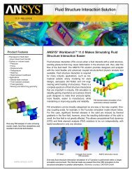
A boundary layer with 10 rows is placed at the cylinder wall using the calculated value of First Cell Height.
The edges are meshed using the First Cell Height and the calculated number of intervals. The entire domain
is meshed using a map scheme (Figure 2.2).
Figure 2.2: Mesh Generated by FlowLab
c○ Fluent Inc. [FlowLab 1.2], April 16, 2007 3

2.3 Physical Models for FLUENT
The user interface updates based upon whether the steady or unsteady solver is selected. The time step
size, the number of iterations per time step, the total number of time steps, and the convergence limit for
each time step must be specified if the unsteady solver is used. The total number of iterations and the
convergence limit must be specified if the steady solver is used.
Based on the Reynolds number, the following physical models are recommended:
Re < 1000 Laminar flow
1000 ≤ Re ≤ 10000 Low Reynolds number k − ɛ model
Re > 10000 k − ɛ model
Table 2.3: Physical Models Based on Reynolds Number
If turbulence is selected in the Physics form of the Operation menu, the appropriate turbulence model and
wall treatment is applied based upon the Reynolds number.
2.4 Material Properties
The default fluid material is water. The following material properties can be specified:
• Density
• Viscosity
Other materials such as Air, Glycerin, and a User Defined fluid can also be selected.
2.5 Boundary Conditions
The following boundary conditions can be specified:
• Inlet velocity
• Wall roughness *
* To be specified only when the flow is modeled as turbulent.
The following boundary conditions are assigned in FLUENT.
Boundary Assigned As
Cylinder Wall
Inlet Velocity inlet
Side boundaries Periodic
Outlet Pressure outlet
Table 2.4: Boundary Conditions Assigned in FLUENT
4 c○ Fluent Inc. [FlowLab 1.2], April 16, 2007

2.6 Solution
The mesh is exported to FLUENT along with the physical properties and the initial conditions specified.
The material properties and the initial conditions are read through the case file. The frequency at which
the results file (neutral file) is saved is written in the journal file file for the unsteady solver using the
execute command. When the solution is converged or the specified number of iterations is met, FLUENT
writes the case and data files. GAMBIT reads the neutral and .xy plot files for postprocessing.
3 Scope and Limitations
FlowLab automatically sets the time step size such that 50 time iterations are performed in one shedding
cycle. Increasing the time step size may lead to incorrect predictions. It is recommended to use at least 20
time iterations for one cycle of vortex shedding.
Enhanced wall treatment is used for turbulent flow conditions to predict the drag coefficient accurately for
Reynold’s numbers between 1000 to 5000. For a Reynolds number higher than 5000, the cell count and the
simulation run time increases exponentially. To reduce simulation run time at higher Reynold’s numbers,
standard wall functions were imposed at Reynolds number greater than 20000. However, standard wall
functions may lead to inaccurate drag predictions at these higher Reynolds numbers.
Difficulty in obtaining convergence or poor accuracy may result if input values are used outside the upper
and lower limits suggested in the problem overview.
4 Exercise Results
4.1 Reports
The following reports are available:
• Static pressure difference
• Total pressure difference
• Average velocity at the outlet
• Total drag coefficient on the cylinder
• Average shear stress on the cylinder *
* Available only for viscous flow.
4.2 XY Plots
The plots reported by FlowLab include:
• Residuals
• Pressure coefficient distribution over cylinder
• Pressure distribution over cylinder
• X-velocity distribution along center line
• Friction coefficient distribution *
• CD history
c○ Fluent Inc. [FlowLab 1.2], April 16, 2007 5

• CL history
• X-wall shear distribution over cylinder *
• Wall Yplus distribution **
* Available only for viscous flow.
** Available only when the flow is modeled as turbulent.
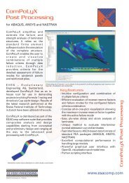
Figure 4.1 represents the distribution of pressure coefficient over the cylinder.
4.3 Contour Plots
Figure 4.1: Pressure Coefficient Distribution at Re = 150
Contours of static pressure, total pressure, velocity, and stream function can be displayed. A velocity vector
plot is also available. All contour plots can be animated if the time dependent solver was used to converge
a solution. Contours of velocity magnitude, x-velocity, y-velocity, turbulence intensity and dissipation rate,
stream function, and temperature can be displayed.
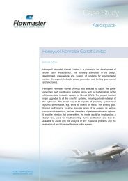
Figure 4.2 represents velocity contours at a Reynolds number of 150, showing a time dependent solution.
6 c○ Fluent Inc. [FlowLab 1.2], April 16, 2007

5 Verification of Results
Figure 4.2: Velocity Contours for Re = 150 at time = 4000 s
Table 5.1 represents predicted drag coefficient as a function of Reynolds number. These results were obtained
using default settings for geometry and material properties with the fine mesh option. The desired Reynolds
number was obtained by varying the inlet velocity.
Re Computed Drag Experimental
Coefficient Results [1]
1 14.87 13.0
40 1.715 1.8
150 1.33 1.5
500 1.35 1.2
1000 1.115 0.9
5000 1.021 0.98
1e06 0.27 0.25
Table 5.1: Computed Vs. Experimental Values Drag Coefficient
The frequency of vortex shedding behind the cylinder is characterized by the Strouhal number, given by:
St = fD
U∞
c○ Fluent Inc. [FlowLab 1.2], April 16, 2007 7
(5-1)

where,
f = frequency of vortex shedding
U∞ = approach velocity of the fluid
D = diameter of the cylinder
Strouhal number verification has been performed for a Reynolds number of 150 with a cylinder diameter
0.1 m and an inlet velocity of 0.0015 m/s. For a Reynolds number of 150, the experimentally value of the
Strouhal number is approximately 0.172 [2]. The time period of the flow oscillation predicted by FlowLab
is approximately 385 s, which is evaluated by plotting the lift history over the cylinder (Figure 5.1). The
numerically predicted value of Strouhal number for this case is 0.173, which differs by 0.64% from the
experimentally determined value.
6 Sample Problems
6.1 Inviscid Case
Figure 5.1: Time History of Lift Coefficient
1. Run time dependent cases using the inviscid option for several velocity values.
2. Plot pressure coefficient versus position and compare with theory.
3. Explain how and why the local pressure varies around the sides of the cylinder.
4. What is the drag force acting on the cylinder? How is it determined?
8 c○ Fluent Inc. [FlowLab 1.2], April 16, 2007

6.2 Viscous (Viscid) Case
1. Set the Reynolds number to 150 and run a time dependent case using the viscous flow option.
2. Compare predicted drag coefficient with the corresponding theoretical value.
3. How does pressure coefficient distribution vary between the viscid and inviscid cases?
4. Plot velocity vectors and evaluate the flow pattern around the cylinder.
5. Compare the drag coefficient values with experimental data or correlation over a Reynolds number
range of 1 to 1.0e+6.
6. Observe velocity vectors as Reynolds number increases.
7. Explain why the pressure distribution profile flattens out at the back of the cylinder, and compare
the pressure distribution profile with the velocity vector field assessing the region of flow separation.
8. Animate the velocity contour results and review vortex shedding behavior.
7 Reference
[1] Anderson, J.D., “Fundamentals of Aerodynamics”, 2 nd Ed., Ch. 3: pp. 229.
[2] Shames, I. H., “Mechanics of Fluid”, 3 rd Ed., Ch. 13: pp. 669-675.
c○ Fluent Inc. [FlowLab 1.2], April 16, 2007 9