Derivatives - Pauls Online Math Notes

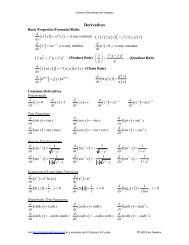
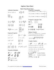
Calculus Cheat Sheet
Derivatives
Definition and Notation
If y = f ( x)
then the derivative is defined to be f ( x)
If y = f ( x)
then all of the following are
equivalent notations for the derivative.
df dy d
f¢ ( x) = y¢
= = = f ( x)
= Df x
dx dx dx
If y = f ( x)
then,
1. m f¢
( a)
( ) ( )
= is the slope of the tangent
line to y = f ( x)
at x = aand the
equation of the tangent line at x = a is
y = f a + f¢
a x- a .
given by ( ) ( )( )
If f ( x ) and ( )
¢ ¢
1. ( cf ) = cf ( x)
( + ) - ( )
¢ = .
h
h ® 0
f
lim
x h f x
If y = f ( x)
all of the following are equivalent
notations for derivative evaluated at x = a.
df dy
f¢ ( a) = y¢
= = = Df ( a)
x=
a
dx dx
x= a x=
a
Interpretation of the Derivative
f¢ a is the instantaneous rate of
2. ( )
change of f ( x ) at x = a.
3. If f ( x ) is the position of an object at
time x then f¢ ( a)
is the velocity of
the object at x = a.
Basic Properties and Formulas
g x are differentiable functions (the derivative exists), c and n are any real numbers,
¢ ¢ ¢
2. ( f ± g) = f ( x) ± g ( x)
3. ( )
fg ¢ = f¢ g+ fg¢
– Product Rule
æ f ö
¢
f¢ g-
fg¢
4. ç =
2
g
÷
– Quotient Rule
è ø g
d
( x ) = 1
dx
d
( sinx)
= cos x
dx
d
( cosx)
=- sin x
dx
d
2
( tanx)
= sec x
dx
d
( secx)
= secxtan
x
dx
d
dx
d x
n nx
n-
= – Power Rule
dx
d
( f ( g x )) = f¢ g( x)
g¢
x
dx
This is the Chain Rule
5. ( c ) = 0
Common Derivatives
d
( cscx)
=- cscxcot
x
dx
d
2
( cotx)
=- csc x
dx
d -1
1
( sin x)
=
dx
2
1-
x
d -1
1
( cos x)
=-
dx
2
1-x
d -1
1
( tan x)
2
dx 1 x
6. ( )
1
7. ( )
( ) ( )
d a a a
x x
( ) = ln( )
dx
d x x
( e ) = e
dx
d 1
( ( x)
) x
dx x
d 1
( x ) = x¹
dx x
d
1
= ( a ( x)
)
+
ln = , > 0
ln , 0
log = , x > 0
dx xlna
Calculus Cheat Sheet
Chain Rule Variants
The chain rule applied to some specific functions.
d
n
n-1
d
1. ( éf ( x)
ù ) = né f ( x) ù f¢
( x)
dx
ë û ë û
5. ( coséf ( x)
) f ( x) sin f ( x)
dx
ë ùû =- ¢ éë ùû
d f ( x)
f ( x)
d
2
2. ( e ) = f¢
( x)
e
6. ( tanéf ( x)
) f ( x) sec f ( x)
dx
dx
ë ùû = ¢ éë ùû
d
f¢
( x)
d
3. ( ln éf
( x)
ù)
=
dx
ë û
7. sec[ f ( x) ] = f ¢ ( x) sec f ( x) tan f ( x)
f ( x)
dx
d
d 1
f ( x)
4. ( sinéf ( x)
ù) = f¢
( x) cos éf ( x)
ù
8. ( tan
- éf
( x)
)
¢
2
dx
ë û ë û dx
ë ùû
=
1+éëf ( x)
ùû
( ) [ ] [ ]
Higher Order Derivatives
The Second Derivative is denoted as
The n th Derivative is denoted as
2
n
( 2
( ) ) d f
( n
f¢¢ x = f ( x)
= and is defined as
) d f
f
2
( x)
= and is defined as
n
dx
dx
f¢¢ ( x) = ( f¢
( x ))
¢ , i.e. the derivative of the
( n ) ( n- 1
( )
) ¢
f x = ( f ( x)
), i.e. the derivative of
first derivative, f¢ ( x)
.
the (n-1) st n-1
derivative, f x .
( )
( )
Implicit Differentiation
+ xy = sin y + 11x
y = y x here, so products/quotients of x and y
2x-9y
3 2
Find y¢ if e ( ) . Remember ( )
will use the product/quotient rule and derivatives of y will use the chain rule. The “trick” is to
differentiate as normal and every time you differentiate a y you tack on a y¢ (from the chain rule).
After differentiating solve for y¢ .
e
( - y¢ ) +
e
x y + xyy¢ = ( y)
y¢
+
( )
-
x- y
e - ( ) ¢ = -
x-
y
e -
2x-9y
2 2 3
2 9 3 2 cos 11
- y¢ + xy + xyy¢ = y y¢ + Þ y¢
=
2x-9y 2x-9y
2 2 3
2e
9 3 2 cos 11
( )
2xy 9 cos y y 11 2 3xy
3 2 9 2 9 2 2
Critical Points
x c
= is a critical point of f ( )
1. f¢ ( c) = 0 or 2. f ( c)
Increasing/Decreasing – Concave Up/Concave Down
¢ doesn’t exist.
x provided either
Increasing/Decreasing
1. If f¢ ( x) > 0 for all x in an interval I then
f ( x ) is increasing on the interval I.
¢ < for all x in an interval I then
2. If f ( x) 0
f ( x ) is decreasing on the interval I.
¢ = for all x in an interval I then
3. If f ( x) 0
f ( x ) is constant on the interval I.
2x-9y
2 2
11-2e
-3x y
3 2x-9y
2xy-9e
-cos
( y)
Concave Up/Concave Down
f¢¢ x > for all x in an interval I then
1. If ( ) 0
f ( x ) is concave up on the interval I.
¢¢ < for all x in an interval I then
2. If f ( x) 0
f ( x ) is concave down on the interval I.
Inflection Points
x c
= is a inflection point of f ( )
concavity changes at x = c.
x if the
Visit http://tutorial.math.lamar.edu for a complete set of Calculus notes.
© 2005 Paul Dawkins
Visit http://tutorial.math.lamar.edu for a complete set of Calculus notes.
© 2005 Paul Dawkins

Absolute Extrema
1. x c
= is an absolute maximum of f ( x )
if f ( c) ³ f ( x)
for all x in the domain.
= is an absolute minimum of f ( x )
2. x c
if f ( c) £ f ( x)
for all x in the domain.
Fermat’s Theorem
f x has a relative (or local) extrema at
If ( )
x = c, then x c
= is a critical point of ( )
Calculus Cheat Sheet
f x .
Extreme Value Theorem
f x is continuous on the closed interval
If ( )
[ ab , ] then there exist numbers c and d so that,
£ £ , 2. f ( c ) is the abs. max. in
1. a cd , b
[ ab , ] , 3. ( )
f d is the abs. min. in [ , ]
ab .
Finding Absolute Extrema
To find the absolute extrema of the continuous
ab , use the
function f ( x ) on the interval [ ]
following process.
1. Find all critical points of f ( x ) in [ ab , ] .
2. Evaluate f ( x ) at all points found in Step 1.
3. Evaluate f ( a ) and f ( b ) .
4. Identify the abs. max. (largest function
value) and the abs. min.(smallest function
value) from the evaluations in Steps 2 & 3.
Extrema
Relative (local) Extrema
1. x = c is a relative (or local) maximum of
f c ³ f x for all x near c.
f ( x ) if ( ) ( )
2. x = c is a relative (or local) minimum of
f c £ f x for all x near c.
f ( x ) if ( ) ( )
1 st Derivative Test
If x c
= is a critical point of ( )
1. a rel. max. of f ( x ) if f ( x) 0
f x then x = c is
¢ > to the left
of x = c and f¢ ( x) < 0 to the right of x = c.
2. a rel. min. of f ( x ) if f ( x) 0
¢ < to the left
of x = cand f¢ ( x) > 0to the right of x = c.
¢ is
3. not a relative extrema of f ( x ) if f ( x)
the same sign on both sides of x = c.
2 nd Derivative Test
If x c
Mean Value Theorem
,
= is a critical point of f ( x ) such that
f¢ ( c) = 0 then x = c
1. is a relative maximum of f ( x ) if f¢¢ ( c) < 0 .
2. is a relative minimum of f ( x ) if f¢¢ ( c) > 0 .
3. may be a relative maximum, relative
minimum, or neither if f¢¢ ( c) = 0 .
Finding Relative Extrema and/or
Classify Critical Points
1. Find all critical points of f ( x ) .
2. Use the 1 st derivative test or the 2 nd
derivative test on each critical point.
If f ( x ) is continuous on the closed interval [ ab ] and differentiable on the open interval ( ab , )
f ( b) - f ( a)
then there is a number a< c < b such that f¢ ( c)
=
.
b-
a
Newton’s Method
If x
n
is the n th guess for the root/solution of f ( x ) = 0 then (n+1) st guess is
provided f¢ ( x n ) exists.
x
x
f
= - n+ 1 n
¢
f
( xn
)
( x )
n
Calculus Cheat Sheet
Related Rates
Sketch picture and identify known/unknown quantities. Write down equation relating quantities
and differentiate with respect to t using implicit differentiation (i.e. add on a derivative every time
you differentiate a function of t). Plug in known quantities and solve for the unknown quantity.
Ex. A 15 foot ladder is resting against a wall.
The bottom is initially 10 ft away and is being
pushed towards the wall at 1 ft/sec. How fast
4
is the top moving after 12 sec
x¢ is negative because x is decreasing. Using
Pythagorean Theorem and differentiating,
2 2 2
x + y = 15 Þ 2xx¢ + 2yy¢
= 0
1
After 12 sec we have ( )
x = 10- 12 = 7and
so y =
2 2
15 - 7 = 176 . Plug in and solve
for y¢ .
1
7
7( -
4 ) + 176 y¢ = 0 Þ y¢
= ft/sec
4 176
4
Ex. Two people are 50 ft apart when one
starts walking north. The angleθ changes at
0.01 rad/min. At what rate is the distance
between them changing when θ = 0.5 rad
We have θ¢ = 0.01 rad/min. and want to find
x¢ . We can use various trig fcns but easiest is,
x
x¢
secθ = Þ secθ tanθθ¢
=
50 50
We knowθ = 0.05 so plug in θ¢ and solve.
x¢
sec( 0.5) tan( 0.5)( 0.01)
=
50
x¢ = 0.3112 ft/sec
Remember to have calculator in radians!
Optimization
Sketch picture if needed, write down equation to be optimized and constraint. Solve constraint for
one of the two variables and plug into first equation. Find critical points of equation in range of
variables and verify that they are min/max as needed.
Ex. We’re enclosing a rectangular field with
2
Ex. Determine point(s) on y = x + 1 that are
500 ft of fence material and one side of the closest to (0,2).
field is a building. Determine dimensions that
will maximize the enclosed area.
Maximize A= xy subject to constraint of
x+ 2y
= 500 . Solve constraint for x and plug
into area.
A= y( 500-2y)
x = 500-2y
Þ
=
2
500y
- 2y
Differentiate and find critical point(s).
A¢ = 500-4y Þ y = 125
By 2 nd deriv. test this is a rel. max. and so is
the answer we’re after. Finally, find x.
x = 500- 2125 = 250
( )
The dimensions are then 250 x 125.
2 2
2
Minimize f d ( x 0) ( y 2)
= = - + - and the
2
constraint is y = x + 1. Solve constraint for
2
x and plug into the function.
2 2
x y f x y
2
( )
( )
= -1 Þ = + -2
2 2
= y- 1+ y- 2 = y - 3y+
3
Differentiate and find critical point(s).
3
f¢ = 2y-3
Þ y =
2
By the 2 nd derivative test this is a rel. min. and
so all we need to do is find x value(s).
2 3 1 1
x = - 1= Þ x =±
2 2 2
1 3
The 2 points are then ( , 2 2 ) and ( - 1
, 3
2 2 )
Visit http://tutorial.math.lamar.edu for a complete set of Calculus notes.
© 2005 Paul Dawkins
Visit http://tutorial.math.lamar.edu for a complete set of Calculus notes.
© 2005 Paul Dawkins