TEAM FLY - Cromatina

TEAMFLY

BIOINFORMATICS 

SECOND EDITION

METHODS OF 

BIOCHEMICAL ANALYSIS 

Volume 43

BIOINFORMATICS 

A Practical Guide to the 

Analysis of Genes and Proteins 

SECOND EDITION 

Andreas D. Baxevanis 

Genome Technology Branch 

National Human Genome Research Institute 

National Institutes of Health 

Bethesda, Maryland 

USA 

B. F. Francis Ouellette 

Centre for Molecular Medicine and Therapeutics 

Children’s and Women’s Health Centre of British Columbia 

University of British Columbia 

Vancouver, British Columbia 

Canada 

A JOHN WILEY & SONS, INC., PUBLICATION 

New York • Chichester • Weinheim • Brisbane • Singapore • Toronto

Designations used by companies to distinguish their products are often claimed as trademarks. In all instances 

where John Wiley & Sons, Inc., is aware of a claim, the product names appear in initial capital or ALL CAPITAL 

LETTERS. Readers, however, should contact the appropriate companies for more complete information regarding 

trademarks and registration. 

Copyright 2001 by John Wiley & Sons, Inc. All rights reserved. 

No part of this publication may be reproduced, stored in a retrieval system or transmitted in any form or by any means, 

electronic or mechanical, including uploading, downloading, printing, decompiling, recording or otherwise, except as permitted 

under Sections 107 or 108 of the 1976 United States Copyright Act, without the prior written permission of the Publisher. 

Requests to the Publisher for permission should be addressed to the Permissions Department, John Wiley & Sons, Inc., 605 

Third Avenue, New York, NY 10158-0012, (212) 850-6011, fax (212) 850-6008, E-Mail: PERMREQ@WILEY.COM. 

This publication is designed to provide accurate and authoritative information in regard to the 

subject matter covered. It is sold with the understanding that the publisher is not engaged in 

rendering professional services. If professional advice or other expert assistance is required, the 

services of a competent professional person should be sought. 

This title is also available in print as ISBN 0-471-38390-2 (cloth) and ISBN 0-471-38391-0 (paper). 

For more information about Wiley products, visit our website at www.Wiley.com.

ADB dedicates this book to his Goddaughter, Anne Terzian, for her constant kindness, good 

humor, and love—and for always making me smile. 

BFFO dedicates this book to his daughter, Maya. Her sheer joy and delight in the simplest of 

things lights up my world everyday.

CONTENTS 

Foreword ........................................................................................ xiii 

Preface ........................................................................................... xv 

Contributors ................................................................................... xvii 

1 BIOINFORMATICS AND THE INTERNET 1 


Internet Basics .......................................................................... 2 

Connecting to the Internet .......................................................... 4 

Electronic Mail ......................................................................... 7 

File Transfer Protocol ................................................................ 10 

The World Wide Web ................................................................ 13 

Internet Resources for Topics Presented in Chapter 1 .................... 16 

References ................................................................................ 17 

2 THE NCBI DATA MODEL 19 

James M. Ostell, Sarah J. Wheelan, and Jonathan A. Kans 

Introduction .............................................................................. 19 

PUBs: Publications or Perish ...................................................... 24 

SEQ-Ids: What’s in a Name ...................................................... 28 

BIOSEQs: Sequences ................................................................. 31 

BIOSEQ-SETs: Collections of Sequences ..................................... 34 

SEQ-ANNOT: Annotating the Sequence ...................................... 35 

SEQ-DESCR: Describing the Sequence ....................................... 40 

Using the Model ....................................................................... 41 

Conclusions .............................................................................. 43 

References ................................................................................ 43 

3 THE GENBANK SEQUENCE DATABASE 45 

Ilene Karsch-Mizrachi and B. F. Francis Ouellette 

Introduction .............................................................................. 45 

Primary and Secondary Databases ............................................... 47 

Format vs. Content: Computers vs. Humans ................................. 47 

The Database ............................................................................ 49 

vii

viii 

CONTENTS 

The GenBank Flatfile: A Dissection ............................................. 49 

Concluding Remarks .................................................................. 58 


References ................................................................................ 59 

Appendices ............................................................................... 59 

Appendix 3.1 Example of GenBank Flatfile Format .................. 59 

Appendix 3.2 Example of EMBL Flatfile Format ...................... 61 

Appendix 3.3 Example of a Record in CON Division ............... 63 

4 SUBMITTING DNA SEQUENCES TO THE DATABASES 65 

Jonathan A. Kans and B. F. Francis Ouellette 

Introduction .............................................................................. 65 

Why, Where, and What to Submit ............................................. 66 

DNA/RNA ................................................................................ 67 

Population, Phylogenetic, and Mutation Studies ............................ 69 

Protein-Only Submissions ........................................................... 69 

How to Submit on the World Wide Web ...................................... 70 

How to Submit with Sequin ....................................................... 70 

Updates .................................................................................... 77 

Consequences of the Data Model ................................................ 77 

EST/STS/GSS/HTG/SNP and Genome Centers ............................. 79 


Contact Points for Submission of Sequence Data to 

DDBJ/EMBL/GenBank ........................................................... 80 


References ................................................................................ 81 

5 STRUCTURE DATABASES 83 

Christopher W. V. Hogue 

Introduction to Structures ........................................................... 83 

PDB: Protein Data Bank at the Research Collaboratory for 

Structural Bioinformatics (RCSB) ............................................ 87 

MMDB: Molecular Modeling Database at NCBI .......................... 91 

Stucture File Formats ................................................................. 94 

Visualizing Structural Information ............................................... 95 

Database Structure Viewers ........................................................ 100 

Advanced Structure Modeling ..................................................... 103 

Structure Similarity Searching ..................................................... 103 


Problem Set .............................................................................. 107 

References ................................................................................ 107 

6 GENOMIC MAPPING AND MAPPING DATABASES 111 

Peter S. White and Tara C. Matise 

Interplay of Mapping and Sequencing ......................................... 112 

Genomic Map Elements ............................................................. 113

CONTENTS 

ix 

Types of Maps .......................................................................... 115 

Complexities and Pitfalls of Mapping .......................................... 120 

Data Repositories ...................................................................... 122 

Mapping Projects and Associated Resources ................................. 127 

Practical Uses of Mapping Resources .......................................... 142 


Problem Set .............................................................................. 148 

References ................................................................................ 149 

7 INFORMATION RETRIEVAL FROM BIOLOGICAL 

DATABASES 155 


Integrated Information Retrieval: The Entrez System ..................... 156 

LocusLink ................................................................................ 172 

Sequence Databases Beyond NCBI ............................................. 178 

Medical Databases ..................................................................... 181 


Problem Set .............................................................................. 184 

References ................................................................................ 185 

8 SEQUENCE ALIGNMENT AND DATABASE SEARCHING 187 

Gregory D. Schuler 

Introduction .............................................................................. 187 

The Evolutionary Basis of Sequence Alignment ............................ 188 

The Modular Nature of Proteins .................................................. 190 

Optimal Alignment Methods ....................................................... 193 

Substitution Scores and Gap Penalties ......................................... 195 

Statistical Significance of Alignments .......................................... 198 

Database Similarity Searching ..................................................... 198 

FASTA ..................................................................................... 200 

BLAST .................................................................................... 202 

Database Searching Artifacts ....................................................... 204 

Position-Specific Scoring Matrices .............................................. 208 

Spliced Alignments .................................................................... 209 

Conclusions .............................................................................. 210 


References ................................................................................ 212 

9 CREATION AND ANALYSIS OF PROTEIN MULTIPLE 

SEQUENCE ALIGNMENTS 215 

Geoffrey J. Barton 

Introduction .............................................................................. 215 

What is a Multiple Alignment, and Why Do It ........................... 216 

Structural Alignment or Evolutionary Alignment ......................... 216 

How to Multiply Align Sequences ............................................... 217

x 

CONTENTS 

Tools to Assist the Analysis of Multiple Alignments ..................... 222 

Collections of Multiple Alignments ............................................. 227 


Problem Set .............................................................................. 229 

References ................................................................................ 230 

10 PREDICTIVE METHODS USING DNA SEQUENCES 233 


GRAIL ..................................................................................... 235 

FGENEH/FGENES .................................................................... 236 

MZEF ...................................................................................... 238 

GENSCAN ............................................................................... 240 

PROCRUSTES ......................................................................... 241 

How Well Do the Methods Work .............................................. 246 

Strategies and Considerations ...................................................... 248 

Internet Resources for Topics Presented in Chapter 10 .................. 250 

Problem Set .............................................................................. 251 

References ................................................................................ 251 

11 PREDICTIVE METHODS USING PROTEIN SEQUENCES 253 

Sharmila Banerjee-Basu and Andreas D. Baxevanis 

Protein Identity Based on Composition ........................................ 254 

Physical Properties Based on Sequence ........................................ 257 

Motifs and Patterns .................................................................... 259 

Secondary Structure and Folding Classes ..................................... 263 

Specialized Structures or Features ............................................... 269 

Tertiary Structure ....................................................................... 274 


Problem Set .............................................................................. 278 

References ................................................................................ 279 

TEAMFLY 

12 EXPRESSED SEQUENCE TAGS (ESTs) 283 

Tyra G. Wolfsberg and David Landsman 

What is an EST ....................................................................... 284 

EST Clustering .......................................................................... 288 

TIGR Gene Indices .................................................................... 293 

STACK .................................................................................... 293 

ESTs and Gene Discovery .......................................................... 294 

The Human Gene Map .............................................................. 294 

Gene Prediction in Genomic DNA .............................................. 295 

ESTs and Sequence Polymorphisms ............................................ 296 

Assessing Levels of Gene Expression Using ESTs ........................ 296 


Problem Set .............................................................................. 298 

References ................................................................................ 299 

Team-Fly ®

CONTENTS 

xi 

13 SEQUENCE ASSEMBLY AND FINISHING METHODS 303 

Rodger Staden, David P. Judge, and James K. Bonfield 

The Use of Base Cell Accuracy Estimates or Confidence Values .... 305 

The Requirements for Assembly Software .................................... 306 

Global Assembly ....................................................................... 306 

File Formats ............................................................................. 307 

Preparing Readings for Assembly ................................................ 308 

Introduction to Gap4 .................................................................. 311 

The Contig Selector ................................................................... 311 

The Contig Comparator .............................................................. 312 

The Template Display ................................................................ 313 

The Consistency Display ............................................................ 316 

The Contig Editor ..................................................................... 316 

The Contig Joining Editor .......................................................... 319 

Disassembling Readings ............................................................. 319 

Experiment Suggestion and Automation ....................................... 319 



Problem Set .............................................................................. 322 

References ................................................................................ 322 

14 PHYLOGENETIC ANALYSIS 323 

Fiona S. L. Brinkman and Detlef D. Leipe 

Fundamental Elements of Phylogenetic Models ............................ 325 

Tree Interpretation—The Importance of Identifying Paralogs 

and Orthologs ........................................................................ 327 

Phylogenetic Data Analysis: The Four Steps ................................ 327 

Alignment: Building the Data Model ........................................... 329 

Alignment: Extraction of a Phylogenetic Data Set ........................ 333 

Determining the Substitution Model ............................................ 335 

Tree-Building Methods ............................................................... 340 

Distance, Parsimony, and Maximum Likelihood: What’s the 

Difference ............................................................................ 345 

Tree Evaluation ......................................................................... 346 

Phylogenetics Software .............................................................. 348 

Internet-Accessible Phylogenetic Analysis Software ...................... 354 

Some Simple Practical Considerations ......................................... 356 


References ................................................................................ 357 

15 COMPARATIVE GENOME ANALYSIS 359 

Michael Y. Galperin and Eugene V. Koonin 

Progress in Genome Sequencing ................................................. 360 

Genome Analysis and Annotation ................................................ 366 

Application of Comparative Genomics—Reconstruction of 

Metabolic Pathways ............................................................... 382 

Avoiding Common Problems in Genome Annotation ..................... 385

xii 

CONTENTS 

Conclusions .............................................................................. 387 


Problems for Additional Study .................................................... 389 

References ................................................................................ 390 

16 LARGE-SCALE GENOME ANALYSIS 393 

Paul S. Meltzer 

Introduction .............................................................................. 393 

Technologies for Large-Scale Gene Expression ............................. 394 

Computational Tools for Expression Analysis ............................... 399 

Hierarchical Clustering ............................................................... 407 

Prospects for the Future ............................................................. 409 


References ................................................................................ 410 

17 USING PERL TO FACILITATE BIOLOGICAL ANALYSIS 413 

Lincoln D. Stein 

Getting Started .......................................................................... 414 

How Scripts Work ..................................................................... 416 

Strings, Numbers, and Variables .................................................. 417 

Arithmetic ................................................................................ 418 

Variable Interpolation ................................................................. 419 

Basic Input and Output .............................................................. 420 

Filehandles ............................................................................... 422 

Making Decisions ...................................................................... 424 

Conditional Blocks .................................................................... 427 

What is Truth .......................................................................... 430 

Loops ....................................................................................... 430 

Combining Loops with Input ...................................................... 432 

Standard Input and Output ......................................................... 433 

Finding the Length of a Sequence File ........................................ 435 

Pattern Matching ....................................................................... 436 

Extracting Patterns ..................................................................... 440 

Arrays ...................................................................................... 441 

Arrays and Lists ........................................................................ 444 

Split and Join ............................................................................ 444 

Hashes ..................................................................................... 445 

A Real-World Example .............................................................. 446 

Where to Go From Here ............................................................ 449 


Suggested Reading .................................................................... 449 

Glossary .......................................................................................... 451 

Index ............................................................................................... 457

FOREWORD 

I am writing these words on a watershed day in molecular biology. This morning, a 

paper was officially published in the journal Nature reporting an initial sequence and 

analysis of the human genome. One of the fruits of the Human Genome Project, the 

paper describes the broad landscape of the nearly 3 billion bases of the euchromatic 

portion of the human chromosomes. 

In the most narrow sense, the paper was the product of a remarkable international 

collaboration involving six countries, twenty genome centers, and more than a thousand 

scientists (myself included) to produce the information and to make it available 

to the world freely and without restriction. 

In a broader sense, though, the paper is the product of a century-long scientific 

program to understand genetic information. The program began with the rediscovery 

of Mendel’s laws at the beginning of the 20th century, showing that information was 

somehow transmitted from generation to generation in discrete form. During the first 

quarter-century, biologists found that the cellular basis of the information was the 

chromosomes. During the second quarter-century, they discovered that the molecular 

basis of the information was DNA. During the third quarter-century, they unraveled 

the mechanisms by which cells read this information and developed the recombinant 

DNA tools by which scientists can do the same. During the last quarter-century, 

biologists have been trying voraciously to gather genetic information-first from 

genes, then entire genomes. 

The result is that biology in the 21st century is being transformed from a purely 

laboratory-based science to an information science as well. The information includes 

comprehensive global views of DNA sequence, RNA expression, protein interactions 

or molecular conformations. Increasingly, biological studies begin with the study of 

huge databases to help formulate specific hypotheses or design large-scale experiments. 

In turn, laboratory work ends with the accumulation of massive collections 

of data that must be sifted. These changes represent a dramatic shift in the biological 

sciences. 

One of the crucial steps in this transformation will be training a new generation 

of biologists who are both computational scientists and laboratory scientists. This 

major challenge requires both vision and hard work: vision to set an appropriate 

agenda for the computational biologist of the future and hard work to develop a 

curriculum and textbook. 

James Watson changed the world with his co-discovery of the double-helical 

structure of DNA in 1953. But, he also helped train a new generation to inhabit that 

new world in the 1960s and beyond through his textbook, The Molecular Biology 

of the Gene. Discovery and teaching go hand-in-hand in changing the world. 

xiii

xiv 

FOREWORD 

In this book, Andy Baxevanis and Francis Ouellette have taken on the tremendously 

important challenge of training the 21st century computational biologist. Toward 

this end, they have undertaken the difficult task of organizing the knowledge 

in this field in a logical progression and presenting it in a digestible form. And, they 

have done an excellent job. This fine text will make a major impact on biological 

research and, in turn, on progress in biomedicine. We are all in their debt. 

February 15, 2001 

Cambridge, Massachusetts 

Eric S. Lander

PREFACE 

With the advent of the new millenium, the scientific community marked a significant 

milestone in the study of biology—the completion of the ‘‘working draft’’ of the 

human genome. This work, which was chronicled in special editions of Nature and 

Science in early 2001, signals a new beginning for modern biology, one in which 

the majority of biological and biomedical research would be conducted in a 

‘‘sequence-based’’ fashion. This new approach, long-awaited and much-debated, 

promises to quickly lead to advances not only in the understanding of basic biological 

processes, but in the prevention, diagnosis, and treatment of many genetic and genomic 

disorders. While the fruits of sequencing the human genome may not be 

known or appreciated for another hundred years or more, the implications to the 

basic way in which science and medicine will be practiced in the future are staggering. 

The availability of this flood of raw information has had a significant effect 

on the field of bioinformatics as well, with a significant amount of effort being spent 

on how to effectively and efficiently warehouse and access these data, as well as on 

new methods aimed at mining this warehoused data in order to make novel biological 

discoveries. 

This new edition of Bioinformatics attempts to keep up with the quick pace of 

change in this field, reinforcing concepts that have stood the test of time while 

making the reader aware of new approaches and algorithms that have emerged since 

the publication of the first edition. Based on our experience both as scientists and 

as teachers, we have tried to improve upon the first edition by introducing a number 

of new features in the current version. Five chapters have been added on topics that 

have emerged as being important enough in their own right to warrant distinct and 

separate discussion: expressed sequence tags, sequence assembly, comparative genomics, 

large-scale genome analysis, and BioPerl. We have also included problem 

sets at the end of most of the chapters with the hopes that the readers will work 

through these examples, thereby reinforcing their command of the concepts presented 

therein. The solutions to these problems are available through the book’s Web site, 

at www.wiley.com/bioinformatics. We have been heartened by the large number of 

instructors who have adopted the first edition as their book of choice, and hope that 

these new features will continue to make the book useful both in the classroom and 

at the bench. 

There are many individuals we both thank, without whose efforts this volume 

would not have become a reality. First and foremost, our thanks go to all of the 

authors whose individual contributions make up this book. The expertise and professional 

viewpoints that these individuals bring to bear go a long way in making 

this book’s contents as strong as it is. That, coupled with their general good- 

xv

xvi 

PREFACE 

naturedness under tight time constraints, has made working with these men and 

women an absolute pleasure. 

Since the databases and tools discussed in this book are unique in that they are 

freely shared amongst fellow academics, we would be remiss if we did not thank all 

of the people who, on a daily basis, devote their efforts to curating and maintaining 

the public databases, as well as those who have developed the now-indispensible 

tools for mining the data contained in those databases. As we pointed out in the 

preface to the first edition, the bioinformatics community is truly unique in that the 

esprit de corps characterizing this group is one of openness, and this underlying 

philosophy is one that has enabled the field of bioinformatics to make the substantial 

strides that it has in such a short period of time. 

We also thank our editor, Luna Han, for her steadfast patience and support 

throughout the entire process of making this new edition a reality. Through our 

extended discussions both on the phone and in person, and in going from deadline 

to deadline, we’ve developed a wonderful relationship with Luna, and look forward 

to working with her again on related projects in the future. We also would like to 

thank Camille Carter and Danielle Lacourciere at Wiley for making the entire copyediting 

process a quick and (relatively) painless one, as well as Eloise Nelson for 

all of her hard work in making sure all of the loose ends came together on schedule. 

BFFO would like to acknowledge the continued support of Nancy Ryder. Nancy 

is not only a friend, spouse, and mother to our daughter Maya, but a continuous 

source of inspiration to do better, and to challenge; this is something that I try to do 

every day, and her love and support enables this. BFFO also wants to acknowledge 

the continued friendship and support from ADB throughout both of these editions. 

It has been an honor and a privilege to be a co-editor with him. Little did we know 

seven years ago, in the second basement of the Lister Hill Building at NIH where 

we shared an office, that so many words would be shared between our respective 

computers. 

ADB would also like to specifically thank Debbie Wilson for all of her help 

throughout the editing process, whose help and moral support went a long way in 

making sure that this project got done the right way the first time around. I would 

also like to extend special thanks to Jeff Trent, who I have had the pleasure of 

working with for the past several years and with whom I’ve developed a special 

bond, both professionally and personally. Jeff has enthusiastically provided me the 

latitude to work on projects like these and has been a wonderful colleague and friend, 

and I look forward to our continued associations in the future. 


B. F. Francis Ouellette

CONTRIBUTORS 

Sharmila Banerjee-Basu, Genome Technology Branch, National Human Genome 

Research Institute, National Institutes of Health, Bethesda, Maryland 

Geoffrey J. Barton, European Molecular Biology Laboratory, European Bioinformatics 

Institute, Wellcome Trust Genome Campus, Hinxton, Cambridge, United 

Kingdom 

Andreas D. Baxevanis, Genome Technology Branch, National Human Genome Research 

Institute, National Institutes of Health, Bethesda, Maryland 

James K. Bonfield, Medical Research Council, Laboratory of Molecular Biology, 

Cambridge, United Kingdom 

Fiona S. L. Brinkman, Department of Microbiology and Immunology, University 

of British Columbia, Vancouver, British Columbia, Canada 

Michael Y. Galperin, National Center for Biotechnology Information, National Library 

of Medicine, National Institutes of Health, Bethesda, Maryland 

Christopher W. V. Hogue, Samuel Lunenfeld Research Institute, Mount Sinai Hospital, 

Toronto, Ontario, Canada 

David P. Judge, Department of Biochemistry, University of Cambridge, Cambridge, 

United Kingdom 

Jonathan A. Kans, National Center for Biotechnology Information, National Library 


Ilene Karsch-Mizrachi, National Center for Biotechnology Information, National 

Library of Medicine, National Institutes of Health, Bethesda, Maryland 

Eugene V. Koonin, National Center for Biotechnology Information, National Library 


David Landsman, Computational Biology Branch, National Center for Biotechnology 

Information, National Library of Medicine, National Institutes of Health, Bethesda, 

Maryland 

Detlef D. Leipe, National Center for Biotechnology Information, National Library 


Tara C. Matise, Department of Genetics, Rutgers University, New Brunswick, New 

Jersey 

xvii

xviii 

CONTRIBUTORS 

Paul S. Meltzer, Cancer Genetics Branch, National Human Genome Research Institute, 

National Institutes of Health, Bethesda, Maryland 

James M. Ostell, National Center for Biotechnology Information, National Library 


B. F. Francis Ouellette, Centre for Molecular Medicine and Therapeutics, Children’s 

and Women’s Health Centre of British Columbia, The University of British Columbia, 

Vancouver, British Columbia, Canada 

Gregory D. Schuler, National Center for Biotechnology Information, National Library 


Rodger Staden, Medical Research Council, Laboratory of Molecular Biology, Cambridge, 

United Kingdom 

Lincoln D. Stein, The Cold Spring Harbor Laboratory, Cold Spring Harbor, New 

York 

Sarah J. Wheelan, National Center for Biotechnology Information, National Library 

of Medicine, National Institutes of Health, Bethesda, Maryland and Department 

of Molecular Biology and Genetics, The Johns Hopkins School of Medicine, Baltimore, 

Maryland 

Peter S. White, Department of Pediatrics, University of Pennsylvania, Philadelphia, 

Pennsylvania 

Tyra G. Wolfsberg, Genome Technology Branch, National Human Genome Research 

Institute, National Institutes of Health, Bethesda, Maryland

1 

BIOINFORMATICS AND 

THE INTERNET 






Bioinformatics represents a new, growing area of science that uses computational 

approaches to answer biological questions. Answering these questions requires that 

investigators take advantage of large, complex data sets (both public and private) in 

a rigorous fashion to reach valid, biological conclusions. The potential of such an 

approach is beginning to change the fundamental way in which basic science is done, 

helping to more efficiently guide experimental design in the laboratory. 

With the explosion of sequence and structural information available to researchers, 

the field of bioinformatics is playing an increasingly large role in the study of 

fundamental biomedical problems. The challenge facing computational biologists 

will be to aid in gene discovery and in the design of molecular modeling, site-directed 

mutagenesis, and experiments of other types that can potentially reveal previously 

unknown relationships with respect to the structure and function of genes and proteins. 

This challenge becomes particularly daunting in light of the vast amount of 

data that has been produced by the Human Genome Project and other systematic 

sequencing efforts to date. 

Before embarking on any practical discussion of computational methods in solving 

biological problems, it is necessary to lay the common groundwork that will 

enable users to both access and implement the algorithms and tools discussed in this 

book. We begin with a review of the Internet and its terminology, discussing major 

Internet protocol classes as well, without becoming overly engaged in the engineering 

1

2 BIOINFORMATICS AND THE INTERNET 

minutiae underlying these protocols. A more in-depth treatment on the inner workings 

of these protocols may be found in a number of well-written reference books intended 

for the lay audience (Rankin, 1996; Conner-Sax and Krol, 1999; Kennedy, 1999). 

This chapter will also discuss matters of connectivity, ranging from simple modem 

connections to digital subscriber lines (DSL). Finally, we will address one of the 

most common problems that has arisen with the proliferation of Web pages throughout 

the world—finding useful information on the World Wide Web. 

INTERNET BASICS 

Despite the impression that it is a single entity, the Internet is actually a network of 

networks, composed of interconnected local and regional networks in over 100 countries. 

Although work on remote communications began in the early 1960s, the true 

origins of the Internet lie with a research project on networking at the Advanced 

Research Projects Agency (ARPA) of the US Department of Defense in 1969 named 

ARPANET. The original ARPANET connected four nodes on the West Coast, with 

the immediate goal of being able to transmit information on defense-related research 

between laboratories. A number of different network projects subsequently surfaced, 

with the next landmark developments coming over 10 years later. In 1981, BITNET 

(‘‘Because It’s Time’’) was introduced, providing point-to-point connections between 

universities for the transfer of electronic mail and files. In 1982, ARPA introduced 

the Transmission Control Protocol (TCP) and the Internet Protocol (IP); TCP/IP 

allowed different networks to be connected to and communicate with one another, 

creating the system in place today. A number of references chronicle the development 

of the Internet and communications protocols in detail (Quarterman, 1990; Froehlich 

and Kent, 1991; Conner-Sax and Krol, 1999). Most users, however, are content to 

leave the details of how the Internet works to their systems administrators; the relevant 

fact to most is that it does work. 

Once the machines on a network have been connected to one another, there 

needs to be an unambiguous way to specify a single computer so that messages and 

files actually find their intended recipient. To accomplish this, all machines directly 

connected to the Internet have an IP number. IP addresses are unique, identifying 

one and only one machine. The IP address is made up of four numbers separated by 

periods; for example, the IP address for the main file server at the National Center 

for Biotechnology Information (NCBI) at the National Institutes of Health (NIH) is 

130.14.25.1. The numbers themselves represent, from left to right, the domain 

(130.14 for NIH), the subnet (.25 for the National Library of Medicine at NIH), and 

the machine itself (.1). The use of IP numbers aids the computers in directing data; 

however, it is obviously very difficult for users to remember these strings, so IP 

addresses often have associated with them a fully qualified domain name (FQDN) 

that is dynamically translated in the background by domain name servers. Going 

back to the NCBI example, rather than use 130.14.25.1 to access the NCBI 

computer, a user could instead use ncbi.nlm.nih.gov and achieve the same 

result. Reading from left to right, notice that the IP address goes from least to most 

specific, whereas the FQDN equivalent goes from most specific to least. The name 

of any given computer can then be thought of as taking the general form computer.domain, 

with the top-level domain (the portion coming after the last period in 

the FQDN) falling into one of the broad categories shown in Table 1.1. Outside the 


Team-Fly ®

INTERNET BASICS 3 

T A B L E 1.1. Top-Level Doman Names 

TOP-LEVEL DOMAIN NAMES 

.com 

.edu 

.gov 

.mil 

.net 

.org 

Commercial site 

Educational site 

Government site 

Military site 

Gateway or network host 

Private (usually not-for-profit) organizations 

EXAMPLES OF TOP-LEVEL DOMAIN NAMES USED OUTSIDE THE UNITED STATES 

.ca 

.ac.uk 

.co.uk 

Canadian site 

Academic site in the United Kingdom 

Commercial site in the United Kingdom 

GENERIC TOP-LEVEL DOMAINS PROPOSED BY IAHC 

.firm 

.shop 

.web 

.arts 

.rec 

.info 

.nom 

Firms or businesses 

Businesses offering goods to purchase (stores) 

Entities emphasizing activities relating to the World Wide Web 

Cultural and entertainment organizations 

Recreational organizations 

Information sources 

Personal names (e.g., yourlastname.nom) 

A complete listing of domain suffixes, including country codes, can be found at http://www.currents.net/ 

resources/directory/noframes/nf.domains.html. 

United States, the top-level domain names may be replaced with a two-letter code 

specifying the country in which the machine is located (e.g., .ca for Canada and .uk 

for the United Kingdom). In an effort to anticipate the needs of Internet users in the 

future, as well as to try to erase the arbitrary line between top-level domain names 

based on country, the now-dissolved International Ad Hoc Committee (IAHC) was 

charged with developing a new framework of generic top-level domains (gTLD). 

The new, recommended gTLDs were set forth in a document entitled The Generic 

Top Level Domain Memorandum of Understanding (gTLD-MOU); these gTLDs are 

overseen by a number of governing bodies and are also shown in Table 1.1. 

The most concrete measure of the size of the Internet lies in actually counting 

the number of machines physically connected to it. The Internet Software Consortium 

(ISC) conducts an Internet Domain Survey twice each year to count these machines, 

otherwise known as hosts. In performing this survey, ISC considers not only how 

many hostnames have been assigned, but how many of those are actually in use; a 

hostname might be issued, but the requestor may be holding the name in abeyance 

for future use. To test for this, a representative sample of host machines are sent a 

probe (a ‘‘ping’’), with a signal being sent back to the originating machine if the 

host was indeed found. The rate of growth of the number of hosts has been phenomenal; 

from a paltry 213 hosts in August 1981, the Internet now has more than 

60 million ‘‘live’’ hosts. The doubling time for the number of hosts is on the order 

of 18 months. At this time, most of this growth has come from the commercial 

sector, capitalizing on the growing popularity of multimedia platforms for advertising 

and communications such as the World Wide Web.


CONNECTING TO THE INTERNET 

Of course, before being able to use all the resources that the Internet has to offer, 

one needs to actually make a physical connection between one’s own computer and 

‘‘the information superhighway.’’ For purposes of this discussion, the elements of 

this connection have been separated into two discrete parts: the actual, physical 

connection (meaning the ‘‘wire’’ running from one’s computer to the Internet backbone) 

and the service provider, who handles issues of routing and content once 

connected. Keep in mind that, in practice, these are not necessarily treated as two 

separate parts—for instance, one’s service provider may also be the same company 

that will run cables or fibers right into one’s home or office. 

Copper Wires, Coaxial Cables, and Fiber Optics 

Traditionally, users attempting to connect to the Internet away from the office had 

one and only one option—a modem, which uses the existing copper twisted-pair 

cables carrying telephone signals to transmit data. Data transfer rates using modems 

are relatively slow, allowing for data transmission in the range of 28.8 to 56 kilobits 

per second (kbps). The problem with using conventional copper wire to transmit data 

lies not in the copper wire itself but in the switches that are found along the way 

that route information to their intended destinations. These switches were designed 

for the efficient and effective transfer of voice data but were never intended to handle 

the high-speed transmission of data. Although most people still use modems from 

their home, a number of new technologies are already in place and will become more 

and more prevalent for accessing the Internet away from hardwired Ethernet networks. 

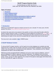
The maximum speeds at which each of the services that are discussed below 

can operate are shown in Figure 1.1. 

The first of these ‘‘new solutions’’ is the integrated services digital network or 

ISDN. The advent of ISDN was originally heralded as the way to bring the Internet 

into the home in a speed-efficient manner; however, it required that special wiring 

be brought into the home. It also required that users be within a fixed distance from 

a central office, on the order of 20,000 feet or less. The cost of running this special, 

dedicated wiring, along with a per-minute pricing structure, effectively placed ISDN 

out of reach for most individuals. Although ISDN is still available in many areas, 

this type of service is quickly being supplanted by more cost-effective alternatives. 

In looking at alternatives that did not require new wiring, cable television providers 

began to look at ways in which the coaxial cable already running into a 

substantial number of households could be used to also transmit data. Cable companies 

are able to use bandwidth that is not being used to transmit television signals 

(effectively, unused channels) to push data into the home at very high speeds, up to 

4.0 megabits per second (Mbps). The actual computer is connected to this network 

through a cable modem, which uses an Ethernet connection to the computer and a 

coaxial cable to the wall. Homes in a given area all share a single cable, in a wiring 

scheme very similar to how individual computers are connected via the Ethernet in 

an office or laboratory setting. Although this branching arrangement can serve to 

connect a large number of locations, there is one major disadvantage: as more and 

more homes connect through their cable modems, service effectively slows down as 

more signals attempt to pass through any given node. One way of circumventing

CONNECTING TO THE INTERNET 5 

35 

30 

25 

Maximum Speed (Mbps) 

Time to Download 20 GB 

GenBank File (days) 

33.3 

20 

15 

14.5 

14.5 

10 

10 

7.1 

5 

0 

Ethernet 

0.2 

ADSL 

0.3 

4 

0.5 

Cable modem 

1.544 

1.2 

T1 

0.4 

4.6 

Satellite 

0.120 

ISDN 

0.120 

0.050 

Cellular wireless 

Telephone modem 

Figure 1.1. Performance of various types of Internet connections, by maximum throughput. 

The numbers indicated in the graph refer to peak performance; often times, the actual 

performance of any given method may be on the order of one-half slower, depending on 

configurations and system conditions. 

this problem is the installation of more switching equipment and reducing the size 

of a given ‘‘neighborhood.’’ 

Because the local telephone companies were the primary ISDN providers, they 

quickly turned their attention to ways that the existing, conventional copper wire 

already in the home could be used to transmit data at high speed. The solution here 

is the digital subscriber line or DSL. By using new, dedicated switches that are 

designed for rapid data transfer, DSL providers can circumvent the old voice switches 

that slowed down transfer speeds. Depending on the user’s distance from the central 

office and whether a particular neighborhood has been wired for DSL service, speeds 

are on the order of 0.8 to 7.1 Mbps. The data transfers do not interfere with voice 

signals, and users can use the telephone while connected to the Internet; the signals 

are ‘‘split’’ by a special modem that passes the data signals to the computer and a 

microfilter that passes voice signals to the handset. There is a special type of DSL 

called asynchronous DSL or ADSL. This is the variety of DSL service that is becoming 

more and more prevalent. Most home users download much more information 

than they send out; therefore, systems are engineered to provide super-fast 

transmission in the ‘‘in’’ direction, with transmissions in the ‘‘out’’ direction being 

5–10 times slower. Using this approach maximizes the amount of bandwidth that 

can be used without necessitating new wiring. One of the advantages of ADSL over 

cable is that ADSL subscribers effectively have a direct line to the central office, 

meaning that they do not have to compete with their neighbors for bandwidth. This, 

of course, comes at a price; at the time of this writing, ADSL connectivity options 

were on the order of twice as expensive as cable Internet, but this will vary from 

region to region. 

Some of the newer technologies involve wireless connections to the Internet. 

These include using one’s own cell phone or a special cell phone service (such as


Ricochet) to upload and download information. These cellular providers can provide 

speeds on the order of 28.8–128 kbps, depending on the density of cellular towers 

in the service area. Fixed-point wireless services can be substantially faster because 

the cellular phone does not have to ‘‘find’’ the closest tower at any given time. Along 

these same lines, satellite providers are also coming on-line. These providers allow 

for data download directly to a satellite dish with a southern exposure, with uploads 

occuring through traditional telephone lines. Along the satellite option has the potential 

to be among the fastest of the options discussed, current operating speeds are 

only on the order of 400 kbps. 

Content Providers vs. ISPs 

Once an appropriately fast and price-effective connectivity solution is found, users 

will then need to actually connect to some sort of service that will enable them to 

traverse the Internet space. The two major categories in this respect are online services 

and Internet service providers (ISPs). Online services, such as America Online 

(AOL) and CompuServe, offer a large number of interactive digital services, including 

information retrieval, electronic mail (E-mail; see below), bulletin boards, and 

‘‘chat rooms,’’ where users who are online at the same time can converse about any 

number of subjects. Although the online services now provide access to the World 

Wide Web, most of the specialized features and services available through these 

systems reside in a proprietary, closed network. Once a connection has been made 

between the user’s computer and the online service, one can access the special features, 

or content, of these systems without ever leaving the online system’s host 

computer. Specialized content can range from access to online travel reservation 

systems to encyclopedias that are constantly being updated—items that are not available 

to nonsubscribers to the particular online service. 

Internet service providers take the opposite tack. Instead of focusing on providing 

content, the ISPs provide the tools necessary for users to send and receive 

E-mail, upload and download files, and navigate around the World Wide Web, finding 

information at remote locations. The major advantage of ISPs is connection speed; 

often the smaller providers offer faster connection speeds than can be had from the 

online services. Most ISPs charge a monthly fee for unlimited use. 

The line between online services and ISPs has already begun to blur. For instance, 

AOL’s now monthly flat-fee pricing structure in the United States allows 

users to obtain all the proprietary content found on AOL as well as all the Internet 

tools available through ISPs, often at the same cost as a simple ISP connection. The 

extensive AOL network puts access to AOL as close as a local phone call in most 

of the United States, providing access to E-mail no matter where the user is located, 

a feature small, local ISPs cannot match. Not to be outdone, many of the major 

national ISP providers now also provide content through the concept of portals. 

Portals are Web pages that can be customized to the needs of the individual user 

and that serve as a jumping-off point to other sources of news or entertainment on 

the Net. In addition, many national firms such as Mindspring are able to match AOL’s 

ease of connectivity on the road, and both ISPs and online providers are becoming 

more and more generous in providing users the capacity to publish their own Web 

pages. Developments such as this, coupled with the move of local telephone and 

cable companies into providing Internet access through new, faster fiber optic net-

ELECTRONIC MAIL 7 

works, foretell major changes in how people will access the Net in the future, 

changes that should favor the end user in both price and performance. 

ELECTRONIC MAIL 

Most people are introduced to the Internet through the use of electronic mail or 

E-mail. The use of E-mail has become practically indispensable in many settings 

because of its convenience as a medium for sending, receiving, and replying to 

messages. Its advantages are many: 

• It is much quicker than the postal service or ‘‘snail mail.’’ 

• Messages tend to be much clearer and more to the point than is the case for 

typical telephone or face-to-face conversations. 

• Recipients have more flexibility in deciding whether a response needs to be 

sent immediately, relatively soon, or at all, giving individuals more control 

over workflow. 

• It provides a convenient method by which messages can be filed or stored. 

• There is little or no cost involved in sending an E-mail message. 

These and other advantages have pushed E-mail to the forefront of interpersonal 

communication in both industry and the academic community; however, users should 

be aware of several major disadvantages. First is the issue of security. As mail travels 

toward its recipient, it may pass through a number of remote nodes, at any one of 

which the message may be intercepted and read by someone with high-level access, 

such as a systems administrator. Second is the issue of privacy. In industrial settings, 

E-mail is often considered to be an asset of the company for use in official communication 

only and, as such, is subject to monitoring by supervisors. The opposite 

is often true in academic, quasi-academic, or research settings; for example, the 

National Institutes of Health’s policy encourages personal use of E-mail within the 

bounds of certain published guidelines. The key words here are ‘‘published guidelines’’; 

no matter what the setting, users of E-mail systems should always find out 

their organization’s policy regarding appropriate use and confidentiality so that they 

may use the tool properly and effectively. An excellent, basic guide to the effective 

use of E-mail (Rankin, 1996) is recommended. 

Sending E-Mail. E-mail addresses take the general form user@computer. 

domain, where user is the name of the individual user and computer.domain specifies 

the actual computer that the E-mail account is located on. Like a postal letter, an 

E-mail message is comprised of an envelope or header, showing the E-mail addresses 

of sender and recipient, a line indicating the subject of the E-mail, and information 

about how the E-mail message actually traveled from the sender to the recipient. 

The header is followed by the actual message, or body, analogous to what would go 

inside a postal envelope. Figure 1.2 illustrates all the components of an E-mail 

message. 

E-mail programs vary widely, depending on both the platform and the needs of 

the users. Most often, the characteristics of the local area network (LAN) dictate 

what types of mail programs can be used, and the decision is often left to systems

Delivery details 

(Envelope) 


Header 

Body 

Received: from dodo.cpmc.columbia.edu (dodo.cpmc.columbia.edu 

[156.111.190.78]) by members.aol.com (8.9.3/8.9.3) with 

ESMTP id RAA13177 for ; Sun, 2 Jan 2000 

17:55:22 -0500 (EST) 

Received: (from phd@localhost) by dodo.cpmc.columbia.edu 

(980427.SGI.8.8.8/980728.SGI.AUTOCF) id RAA90300 for 

scienceguy1@aol.com; Sun, 2 Jan 2000 17:51:20 -0500 (EST) 

Date: Sun, 2 Jan 2000 17:51:20 -0500 (EST) 

Message-ID: 

From: phd@dodo.cpmc.columbia.edu (PredictProtein) 

To: scienceguy1@aol.com 

Subject: PredictProtein 

PredictProtein Help 

PHDsec, PHDacc, PHDhtm, PHDtopology, TOPITS, MaxHom, EvalSec 

Burkhard Rost 

Table of Contents for PP help 

Sender, Recipient, 

and Subject 

1. Introduction 

1. What is it 

2. How does it work 

3. How to use it 

Figure 1.2. Anatomy of an E-mail message, with relevant components indicated. This message 

is an automated reply to a request for help file for the PredictProtein E-mail server. 

administrators rather than individual users. Among the most widely used E-mail 

packages with a graphical user interface are Eudora for the Macintosh and both 

Netscape Messenger and Microsoft Exchange for the Mac, Windows, and UNIX 

platforms. Text-based E-mail programs, which are accessed by logging in to a UNIXbased 

account, include Elm and Pine. 

Bulk E-Mail. As with postal mail, there has been an upsurge in ‘‘spam’’ or 

‘‘junk E-mail,’’ where companies compile bulk lists of E-mail addresses for use in 

commercial promotions. Because most of these lists are compiled from online registration 

forms and similar sources, the best defense for remaining off these bulk 

E-mail lists is to be selective as to whom E-mail addresses are provided. Most 

newsgroups keep their mailing lists confidential; if in doubt and if this is a concern, 

one should ask. 

E-Mail Servers. Most often, E-mail is thought of a way to simply send messages, 

whether it be to one recipient or many. It is also possible to use E-mail as a 

mechanism for making predictions or retrieving records from biological databases. 

Users can send E-mail messages in a format defining the action to be performed to 

remote computers known as servers; the servers will then perform the desired operation 

and E-mail back the results. Although this method is not interactive (in that 

the user cannot adjust parameters or have control over the execution of the method 

in real time), it does place the responsibility for hardware maintenance and software 

upgrades on the individuals maintaining the server, allowing users to concentrate on 

their results instead of on programming. The use of a number of E-mail servers is 

discussed in greater detail in context in later chapters. For most of these servers, 

sending the message help to the server E-mail address will result in a detailed set 

of instructions for using that server being returned, including ways in which queries 

need to be formatted.

ELECTRONIC MAIL 9 

Aliases and Newsgroups. In the example in Figure 1.2, the E-mail message 

is being sent to a single recipient. One of the strengths of E-mail is that a single 

piece of E-mail can be sent to a large number of people. The primary mechanism 

for doing this is through aliases; a user can define a group of people within their 

mail program and give the group a special name or alias. Instead of using individual 

E-mail addresses for all of the people in the group, the user can just send the E-mail 

to the alias name, and the mail program will handle broadcasting the message to 

each person in that group. Setting up alias names is a tremendous time-saver even 

for small groups; it also ensures that all members of a given group actually receive 

all E-mail messages intended for the group. 

The second mechanism for broadcasting messages is through newsgroups. This 

model works slightly differently in that the list of E-mail addresses is compiled and 

maintained on a remote computer through subscriptions, much like magazine subscriptions. 

To participate in a newsgroup discussions, one first would have to subscribe 

to the newsgroup of interest. Depending on the newsgroup, this is done either 

by sending an E-mail to the host server or by visiting the host’s Web site and using 

a form to subscribe. For example, the BIOSCI newsgroups are among the most highly 

trafficked, offering a forum for discussion or the exchange of ideas in a wide variety 

of biological subject areas. Information on how to subscribe to one of the constituent 

BIOSCI newsgroups is posted on the BIOSCI Web site. To actually participate in 

the discussion, one would simply send an E-mail to the address corresponding to 

the group that you wish to reach. For example, to post messages to the computational 

biology newsgroup, mail would simply be addressed to comp-bio@net.bio. 

net, and, once that mail is sent, everyone subscribing to that newsgroup would 

receive (and have the opportunity to respond to) that message. The ease of reaching 

a large audience in such a simple fashion is both a blessing and a curse, so many 

newsgroups require that postings be reviewed by a moderator before they get disseminated 

to the individual subscribers to assure that the contents of the message 

are actually of interest to the readers. 

It is also possible to participate in newsgroups without having each and every 

piece of E-mail flood into one’s private mailbox. Instead, interested participants can 

use news-reading software, such as NewsWatcher for the Macintosh, which provides 

access to the individual messages making up a discussion. The major advantage is 

that the user can pick and choose which messages to read by scanning the subject 

lines; the remainder can be discarded by a single operation. NewsWatcher is an 

example of what is known as a client-server application; the client software (here, 

NewsWatcher) runs on a client computer (a Macintosh), which in turn interacts with 

a machine at a remote location (the server). Client-server architecture is interactive 

in nature, with a direct connection being made between the client and server 

machines. 

Once NewsWatcher is started, the user is presented with a list of newsgroups 

available to them (Fig. 1.3). This list will vary, depending on the user’s location, as 

system administrators have the discretion to allow or to block certain groups at a 

given site. From the rear-most window in the figure, the user double-clicks on the 

newsgroup of interest (here, bionet.genome.arabidopsis), which spawns the window 

shown in the center. At the top of the center window is the current unread message 

count, and any message within the list can be read by double-clicking on that particular 

line. This, in turn, spawns the last window (in the foreground), which shows 

the actual message. If a user decides not to read any of the messages, or is done


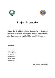
Figure 1.3. Using NewsWatcher to read postings to newsgroups. The list of newsgroups 

that the user has subscribed to is shown in the Subscribed List window (left). The list of 

new postings for the highlighted newsgroup (bionet.genome.arabidopsis) is shown in the 

center window. The window in the foreground shows the contents of the posting selected 

from the center window. 

reading individual messages, the balance of the messages within the newsgroup (center) 

window can be deleted by first choosing Select All from the File menu and then 

selecting Mark Read from the News menu. Once the newsgroup window is closed, 

the unread message count is reset to zero. Every time NewsWatcher is restarted, it 

will automatically poll the news server for new messages that have been created 

since the last session. As with most of the tools that will be discussed in this chapter, 

news-reading capability is built into Web browsers such as Netscape Navigator and 

Microsoft Internet Explorer. 

FILE TRANSFER PROTOCOL 

Despite the many advantages afforded by E-mail in transmitting messages, many 

users have no doubt experienced frustration in trying to transmit files, or attachments, 

along with an E-mail message. The mere fact that a file can be attached to an 

E-mail message and sent does not mean that the recipient will be able to detach, 

decode, and actually use the attached file. Although more cross-platform E-mail 

packages such as Microsoft Exchange are being developed, the use of different E- 

mail packages by people at different locations means that sending files via E-mail 

is not an effective, foolproof method, at least in the short term. One solution to this

FILE TRANSFER PROTOCOL 11 

problem is through the use of a file transfer protocol or FTP. The workings of 

FTP are quite simple: a connection is made between a user’s computer (the client) 

and a remote server, and that connection remains in place for the duration of the 

FTP session. File transfers are very fast, at rates on the order of 5–10 kilobytes per 

second, with speeds varying with the time of day, the distance between the client 

and server machines, and the overall traffic on the network. 

In the ordinary case, making an FTP connection and transferring files requires 

that a user have an account on the remote server. However, there are many files and 

programs that are made freely available, and access to those files does not require 

having an account on each and every machine where these programs are stored. 

Instead, connections are made using a system called anonymous FTP. Under this 

system, the user connects to the remote machine and, instead of entering a username/ 

password pair, types anonymous as the username and enters their E-mail address 

in place of a password. Providing one’s E-mail address allows the server’s system 

administrators to compile access statistics that may, in turn, be of use to those actually 

providing the public files or programs. An example of an anonymous FTP session 

using UNIX is shown in Figure 1.4. 

Although FTP actually occurs within the UNIX environment, Macintosh and PC 

users can use programs that rely on graphical user interfaces (GUI, pronounced 

Figure 1.4. Using UNIX FTP to download a file. An anonymous FTP session is established 

with the molecular biology FTP server at the University of Indiana to download the CLUSTAL 

W alignment program. The user inputs are shown in boldface.


‘‘gooey’’) to navigate through the UNIX directories on the FTP server. Users need 

not have any knowledge of UNIX commands to download files; instead, they select 

from pop-up menus and point and click their way through the UNIX file structure. 

The most popular FTP program on the Macintosh platform for FTP sessions is Fetch. 

A sample Fetch window is shown in Figure 1.5 to illustrate the difference between 

using a GUI-based FTP program and the equivalent UNIX FTP in Figure 1.4. In the 

figure, notice that the Automatic radio button (near the bottom of the second window 

under the Get File button) is selected, meaning that Fetch will determine the appropriate 

type of file transfer to perform. This may be manually overridden by selecting 

either Text or Binary, depending on the nature of the file being transferred. As a 

rule, text files should be transferred as Text, programs or executables as Binary, and 

graphic format files such as PICT and TIFF files as Raw Data. 


Figure 1.5. Using Fetch to download a file. An anonymous FTP session is established with 

the molecular biology FTP server at the University of Indiana (top) to download the 

CLUSTAL W alignment program (bottom). Notice the difference between this GUI-based 

program and the UNIX equivalent illustrated in Figure 1.4. 

Team-Fly ®

THE WORLD WIDE WEB 13 

THE WORLD WIDE WEB 

Although FTP is of tremendous use in the transfer of files from one computer to 

another, it does suffer from some limitations. When working with FTP, once a user 

enters a particular directory, they can only see the names of the directories or files. 

To actually view what is within the files, it is necessary to physically download the 

files onto one’s own computer. This inherent drawback led to the development of a 

number of distributed document delivery systems (DDDS), interactive client-server 

applications that allowed information to be viewed without having to perform a 

download. The first generation of DDDS development led to programs like Gopher, 

which allowed plain text to be viewed directly through a client-server application. 

From this evolved the most widely known and widely used DDDS, namely, the 

World Wide Web. The Web is an outgrowth of research performed at the European 

Nuclear Research Council (CERN) in 1989 that was aimed at sharing research data 

between several locations. That work led to a medium through which text, images, 

sounds, and videos could be delivered to users on demand, anywhere in the world. 

Navigation on the World Wide Web 

Navigation on the Web does not require advance knowledge of the location of the 

information being sought. Instead, users can navigate by clicking on specific text, 

buttons, or pictures. These clickable items are collectively known as hyperlinks. Once 

one of these hyperlinks is clicked, the user is taken to another Web location, which 

could be at the same site or halfway around the world. Each document displayed on 

the Web is called a Web page, and all of the related Web pages on a particular server 

are collectively called a Web site. Navigation strictly through the use of hyperlinks 

has been nicknamed ‘‘Web surfing.’’ 

Users can take a more direct approach to finding information by entering a 

specific address. One of the strengths of the Web is that the programs used to view 

Web pages (appropriately termed browsers) can be used to visit FTP and Gopher 

sites as well, somewhat obviating the need for separate Gopher or FTP applications. 

As such, a unified naming convention was introduced to indicate to the browser 

program both the location of the remote site and, more importantly, the type of 

information at that remote location so that the browser could properly display the 

data. This standard-form address is known as a uniform resource locator, or URL, 

and takes the general form protocol://computer.domain, where protocol specifies the 

type of site and computer.domain specifies the location (Table 1.2). The http used 

for the protocol in World Wide Web URLs stands for hypertext transfer protocol, 

the method used in transferring Web files from the host computer to the client. 

T A B L E 1.2. Uniform Resource Locator (URL) Format 

for Each Type of Transfer Protocol 

General form 

FTP site 

Gopher site 

Web site 

protocol://computer.domain 

ftp://ftp.ncbi.nlm.nih.gov 

gopher://gopher.iubio.indiana.edu 

http://www.nhgri.nih.gov


Browsers 

Browsers, which are used to look at Web pages, are client-server applications that 

connect to a remote site, download the requested information at that site, and display 

the information on a user’s monitor, then disconnecting from the remote host. The 

information retrieved from the remote host is in a platform-independent format 

named hypertext markup language (HTML). HTML code is strictly text-based, and 

any associated graphics or sounds for that document exist as separate files in a 

common format. For example, images may be stored and transferred in GIF format, 

a proprietary format developed by CompuServe for the quick and efficient transfer 

of graphics; other formats, such as JPEG and BMP, may also be used. Because of 

this, a browser can display any Web page on any type of computer, whether it be a 

Macintosh, IBM compatible, or UNIX machine. The text is usually displayed first, 

with the remaining elements being placed on the page as they are downloaded. With 

minor exception, a given Web page will look the same when the same browser is 

used on any of the above platforms. The two major players in the area of browser 

software are Netscape, with their Communicator product, and Microsoft, with Internet 

Explorer. As with many other areas where multiple software products are available, 

the choice between Netscape and Internet Explorer comes down to one of 

personal preference. Whereas the computer literati will debate the fine points of 

difference between these two packages, for the average user, both packages perform 

equally well and offer the same types of features, adequately addressing the Webbrowser 

needs of most users. 

It is worth mentioning that, although the Web is by definition a visually-based 

medium, it is also possible to travel through Web space and view documents without 

the associated graphics. For users limited to line-by-line terminals, a browser called 

Lynx is available. Developed at the University of Kansas, Lynx allows users to use 

their keyboard arrow keys to highlight and select hyperlinks, using their return key 

the same way that Netscape and Internet Explorer users would click their mouse. 

Internet vs. Intranet 

The Web is normally thought of as a way to communicate with people at a distance, 

but the same infrastructure can be used to connect people within an organization. 

Such intranets provide an easily accessible repository of relevant information, capitalizing 

on the simplicity of the Web interface. They also provide another channel 

for broadcast or confidential communication within the organization. Having an intranet 

is of particular value when members of an organization are physically separated, 

whether in different buildings or different cities. Intranets are protected: that 

is, people who are not on the organization’s network are prohibited from accessing 

the internal Web pages; additional protections through the use of passwords are also 

common. 

Finding Information on the World Wide Web 

Most people find information on the Web the old-fashioned way: by word of mouth, 

either using lists such as those preceding the References in the chapters of this book 

or by simply following hyperlinks put in place by Web authors. Continuously clicking 

from page to page can be a highly ineffective way of finding information, though,

THE WORLD WIDE WEB 15 

especially when the information sought is of a very focused nature. One way of 

finding interesting and relevant Web sites is to consult virtual libraries, which are 

curated lists of Web resources arranged by subject. Virtual libraries of special interest 

to biologists include the WWW Virtual Library, maintained by Keith Robison at 

Harvard, and the EBI BioCatalog, based at the European Bioinformatics Institute. 

The URLs for these sites can be found in the list at the end of this chapter. 

It is also possible to directly search the Web by using search engines. A search 

engine is simply a specialized program that can perform full-text or keyword searches 

on databases that catalog Web content. The result of a search is a hyperlinked list 

of Web sites fitting the search criteria from which the user can visit any or all of the 

found sites. However, the search engines use slightly different methods in compiling 

their databases. One variation is the attempt to capture most or all of the text of 

every Web page that the search engine is able to find and catalog (‘‘Web crawling’’). 

Another technique is to catalog only the title of each Web page rather than its entire 

text. A third is to consider words that must appear next to each other or only relatively 

close to one another. Because of these differences in search-engine algorithms, the 

results returned by issuing the same query to a number of different search engines 

can produce wildly different results (Table 1.3). The other important feature of Table 

1.3 is that most of the numbers are exceedingly large, reflecting the overall size of 

the World Wide Web. Unless a particular search engine ranks its results by relevance 

(e.g., by scoring words in a title higher than words in the body of the Web page), 

the results obtained may not be particularly useful. Also keep in mind that, depending 

on the indexing scheme that the search engine is using, the found pages may actually 

no longer exist, leading the user to the dreaded ‘‘404 Not Found’’ error. 

Compounding this problem is the issue of coverage—the number of Web pages 

that any given search engine is actually able to survey and analyze. A comprehensive 

study by Lawrence and Giles (1998) indicates that the coverage provided by any of 

the search engines studied is both small and highly variable. For example, the HotBot 

engine produced 57.5% coverage of what was estimated to be the size of the ‘‘indexable 

Web,’’ whereas Lycos had only 4.41% coverage, a full order of magnitude 

less than HotBot. The most important conclusion from this study was that the extent 

of coverage increased as the number of search engines was increased and the results 

from those individual searches were combined. Combining the results obtained from 

the six search engines examined in this study produced coverage approaching 100%. 

To address this point, a new class of search engines called meta-search engines 

have been developed. These programs will take the user’s query and poll anywhere 

from 5–10 of the ‘‘traditional’’ search engines. The meta-search engine will then 

T A B L E 1.3. Number of Hits Returned for Four Defined Search Queries on Some of the More 

Popular Search and Meta-Search Engines 

Search Term 

Search Engine 

HotBot Excite Infoseek Lycos 

Google 

Meta-Search Engine 

MetaCrawler SavvySearch 

Genetic mapping 

Human genome 

Positional cloning 

Prostate cancer 

478 

13,213 

279 

14,044 

1,040 

34,760 

735 

53,940 

4,326 

15,980 

1,143 

24,376 

9,395 

19,536 

666 

33,538 

7,043 

19,797 

3,987 

23,100 

62 

42 

40 

0 

58 

54 

52 

57


collect the results, filter out duplicates, and return a single, annotated list to the user. 

One big advantage is that the meta-search engines take relevance statistics into account, 

returning much smaller lists of results. Although the hit list is substantially 

smaller, it is much more likely to contain sites that directly address the original 

query. Because the programs must poll a number of different search engines, searches 

conducted this way obviously take longer to perform, but the higher degree of confidence 

in the compiled results for a given query outweighs the extra few minutes 

(and sometimes only seconds) of search time. Reliable and easy-to-use meta-search 

engines include MetaCrawler and Savvy Search. 

INTERNET RESOURCES FOR TOPICS PRESENTED IN CHAPTER 1 

DOMAIN NAMES 

gTLD-MOU 

Internet Software Consortium 

http://www.gtld-mou.org 

http://www.isc.org 

ELECTRONIC MAIL AND NEWSGROUPS 

BIOSCI Newsgroups 

http://www.bio.net/docs/biosci.FAQ.html 

Eudora 

http://www.eudora.com 

Microsoft Exchange 

http://www.microsoft.com/exchange/ 

NewsWatcher 

ftp://ftp.acns.nwu.edu/pub/newswatcher/ 

FILE TRANSFER PROTOCOL 

Fetch 3.0/Mac 

LeechFTP/PC 

INTERNET ACCESS 

America Online 

AT&T 

Bell Atlantic 

Bell Canada 

CompuServe 

Ricochet 

Telus 

Worldcom 

VIRTUAL LIBRARIES 

EBI BioCatalog 

Amos’ WWW Links Page 

NAR Database Collection 

WWW Virtual Library 

WORLD WIDE WEB BROWSERS 

Internet Explorer 

Lynx 

Netscape Navigator 

http://www.dartmouth.edu/pages/softdev/fetch.html 

http://stud.fh-heilbronn.de/j˜debis/leechftp/ 

http://www.aol.com 

http://www.att.com/worldnet 

http://www.verizon.net 

http://www.bell.ca 

http://www.compuserve.com 

http://www.ricochet.net 

http://www.telus.net 

http://www. worldcom.com 

http://www.ebi.ac.uk/biocat/biocat.html 

http://www.expasy.ch/alinks.html 

http://www.nar.oupjournals.org 

http://mcb.harvard.edu/BioLinks.html 

http://explorer.msn.com/home.htm 

ftp://ftp2.cc.ukans.edu/pub/lynx 

http://home.netscape.com 

WORLD WIDE WEB SEARCH ENGINES 

AltaVista 

http://www.altavista.com 

Excite 

http://www.excite.com 

Google 

http://www.google.com

REFERENCES 17 

HotBot 

Infoseek 

Lycos 

Northern Light 

http://hotbot.lycos.com 

http://infoseek.go.com 

http://www.lycos.com 

http://www.northernlight.com 

WORLD WIDE WEB META-SEARCH ENGINES 

MetaCrawler 

http://www.metacrawler.com 

Savvy Search 

http://www.savvysearch.com 

REFERENCES 

Conner-Sax, K., and Krol, E. (1999). The Whole Internet: The Next Generation (Sebastopol, 

CA: O’Reilly and Associates). 

Froehlich, F., and Kent, A. (1991). ARPANET, the Defense Data Network, and Internet. In 

Encyclopedia of Communications (New York: Marcel Dekker). 

Kennedy, A. J. (1999). The Internet: Rough Guide 2000 (London: Rough Guides). 

Lawrence, S., and Giles, C. L. (1998). Searching the World Wide Web. Science 280, 98–100. 

Quarterman, J. (1990). The Matrix: Computer Networks and Conferencing Systems Worldwide 

(Bedford, MA: Digital Press). 

Rankin, B. (1996). Dr. Bob’s Painless Guide to the Internet and Amazing Things You Can 

Do With E-mail (San Francisco: No Starch Press).

2 

THE NCBI DATA MODEL 

James M. Ostell 

National Center for Biotechnology Information 

National Library of Medicine 



Sarah J. Wheelan 

Department of Molecular Biology and Genetics 

The Johns Hopkins School of Medicine 

Baltimore, Maryland 

Jonathan A. Kans 





INTRODUCTION 

Why Use a Data Model 

Most biologists are familiar with the use of animal models to study human diseases. 

Although a disease that occurs in humans may not be found in exactly the same 

form in animals, often an animal disease shares enough attributes with a human 

counterpart to allow data gathered on the animal disease to be used to make inferences 

about the process in humans. Mathematical models describing the forces involved 

in musculoskeletal motions can be built by imagining that muscles are combinations 

of springs and hydraulic pistons and bones are lever arms, and, often times, 

19

20 THE NCBI DATA MODEL 

such models allow meaningful predictions to be made and tested about the obviously 

much more complex biological system under consideration. The more closely and 

elegantly a model follows a real phenomenon, the more useful it is in predicting or 

understanding the natural phenomenon it is intended to mimic. 

In this same vein, some 12 years ago, the National Center for Biotechnology 

Information (NCBI) introduced a new model for sequence-related information. This 

new and more powerful model made possible the rapid development of software and 

the integration of databases that underlie the popular Entrez retrieval system and on 

which the GenBank database is now built (cf. Chapter 7 for more information on 

Entrez). The advantages of the model (e.g., the ability to move effortlessly from the 

published literature to DNA sequences to the proteins they encode, to chromosome 

maps of the genes, and to the three-dimensional structures of the proteins) have been 

apparent for years to biologists using Entrez, but very few biologists understand the 

foundation on which this model is built. As genome information becomes richer and 

more complex, more of the real, underlying data model is appearing in common 

representations such as GenBank files. Without going into great detail, this chapter 

attempts to present a practical guide to the principles of the NCBI data model and 

its importance to biologists at the bench. 

Some Examples of the Model 

The GenBank flatfile is a ‘‘DNA-centered’’ report, meaning that a region of DNA 

coding for a protein is represented by a ‘‘CDS feature,’’ or ‘‘coding region,’’ on the 

DNA. A qualifier (/translation=“MLLYY”) describes a sequence of amino 

acids produced by translating the CDS. A limited set of additional features of the 

DNA, such as mat peptide, are occasionally used in GenBank flatfiles to describe 

cleavage products of the (possibly unnamed) protein that is described by a 

/translation, but clearly this is not a satisfactory solution. Conversely, most 

protein sequence databases present a ‘‘protein-centered’’ view in which the connection 

to the encoding gene may be completely lost or may be only indirectly referenced 

by an accession number. Often times, these connections do not provide the 

exact codon-to-amino acid correspondences that are important in performing mutation 

analysis. 

The NCBI data model deals directly with the two sequences involved: a DNA 

sequence and a protein sequence. The translation process is represented as a link 

between the two sequences rather than an annotation on one with respect to the 

other. Protein-related annotations, such as peptide cleavage products, are represented 

as features annotated directly on the protein sequence. In this way, it becomes very 

natural to analyze the protein sequences derived from translations of CDS features 

by BLAST or any other sequence search tool without losing the precise linkage back 

to the gene. A collection of a DNA sequence and its translation products is called a 

Nuc-prot set, and this is how such data is represented by NCBI. The GenBank flatfile 

format that many readers are already accustomed to is simply a particular style of 

report, one that is more ‘‘human-readable’’ and that ultimately flattens the connected 

collection of sequences back into the familiar one-sequence, DNA-centered view. 

The navigation provided by tools such as Entrez much more directly reflects the 

underlying structure of such data. The protein sequences derived from GenBank 

translations that are returned by BLAST searches are, in fact, the protein sequences 

from the Nuc-prot sets described above.

INTRODUCTION 21 

The standard GenBank format can also hide the multiple-sequence nature of 

some DNA sequences. For example, three genomic exons of a particular gene are 

sequenced, and partial flanking, noncoding regions around the exons may also be 

available, but the full-length sequences of these intronic sequences may not yet be 

available. Because the exons are not in their complete genomic context, there would 

be three GenBank flatfiles in this case, one for each exon. There is no explicit 

representation of the complete set of sequences over that genomic region; these three 

exons come in genomic order and are separated by a certain length of unsequenced 

DNA. In GenBank format there would be a Segment line of the form SEGMENT 1 

of 3 in the first record, SEGMENT 2 of 3 in the second, and SEGMENT 3 of 3 in 

the third, but this only tells the user that the lines are part of some undefined, ordered 

series (Fig. 2.1A). Out of the whole GenBank release, one locates the correct Segment 

records to place together by an algorithm involving the LOCUS name. All segments 

that go together use the same first combination of letters, ending with the numbers 

appropriate to the segment, e.g., HSDDT1, HSDDT2, and HSDDT3. Obviously, this 

complicated arrangement can result in problems when LOCUS names include numbers 

that inadvertently interfere with such series. In addition, there is no one sequence 

record that describes the whole assembled series, and there is no way to describe 

the distance between the individual pieces. There is no segmenting convention in 

the EMBL sequence database at all, so records derived from that source or distributed 

in that format lack even this imperfect information. 

The NCBI data model defines a sequence type that directly represents such a 

segmented series, called a ‘‘segmented sequence.’’ Rather than containing the letters 

A, G, C, and T, the segmented sequence contains instructions on how it can be built 

from other sequences. Considering again the example above, the segmented sequence 

would contain the instructions ‘‘take all of HSDDT1, then a gap of unknown length, 

then all of HSDDT2, then a gap of unknown length, then all of HSDDT3.’’ The 

segmented sequence itself can have a name (e.g., HSDDT), an accession number, 

features, citations, and comments, like any other GenBank record. Data of this type 

are commonly stored in a so-called ‘‘Seg-set’’ containing the sequences HSDDT, 

HSDDT1, HSDDT2, HSDDT3 and all of their connections and features. When the 

GenBank release is made, as in the case of Nuc-prot sets, the Seg-sets are broken 

up into multiple records, and the segmented sequence itself is not visible. However, 

GenBank, EMBL, and DDBJ have recently agreed on a way to represent these 

constructed assemblies, and they will be placed in a new CON division, with CON 

standing for ‘‘contig’’ (Fig. 2.1B). In the Entrez graphical view of segmented sequences, 

the segmented sequence is shown as a line connecting all of its component 

sequences (Fig. 2.1C). 

An NCBI segmented sequence does not require that there be gaps between the 

individual pieces. In fact the pieces can overlap, unlike the case of a segmented 

series in GenBank format. This makes the segmented sequence ideal for representing 

large sequences such as bacterial genomes, which may be many megabases in length. 

This is what currently is done within the Entrez Genomes division for bacterial 

genomes, as well as other complete chromosomes such as yeast. The NCBI Software 

Toolkit (Ostell, 1996) contains functions that can gather the data that a segmented 

sequence refers to ‘‘on the fly,’’ including constituent sequence and features, and this 

information can automatically be remapped from the coordinates of a small, individual 

record to that of a complete chromosome. This makes it possible to provide 

graphical views, GenBank flatfile views, or FASTA views or to perform analyses on



Team-Fly ®

INTRODUCTION 23 

whole chromosomes quite easily, even though data exist only in small, individual 

pieces. This ability to readily assemble a set of related sequences on demand for any 

region of a very large chromosome has already proven to be valuable for bacterial 

genomes. Assembly on demand will become more and more important as larger and 

larger regions are sequenced, perhaps by many different groups, and the notion that 

an investigator will be working on one huge sequence record becomes completely 

impractical. 

What Does ASN.1 Have to Do With It 

The NCBI data model is often referred to as, and confused with, the ‘‘NCBI ASN.1’’ 

or ‘‘ASN.1 Data Model.’’ Abstract Syntax Notation 1 (ASN.1) is an International 

Standards Organization (ISO) standard for describing structured data that reliably 

encodes data in a way that permits computers and software systems of all types to 

reliably exchange both the structure and the content of the entries. Saying that a data 

model is written in ASN.1 is like saying a computer program is written in C or 

FORTRAN. The statement identifies the language; it does not say what the program 

does. The familiar GenBank flatfile was really designed for humans to read, from a 

DNA-centered viewpoint. ASN.1 is designed for a computer to read and is amenable 

to describing complicated data relationships in a very specific way. NCBI describes 

and processes data using the ASN.1 format. Based on that single, common format, 

a number of human-readable formats and tools are produced, such as Entrez, 

GenBank, and the BLAST databases. Without the existence of a common format 

such as this, the neighboring and hard-link relationships that Entrez depends on 

would not be possible. This chapter deals with the structure and content of the NCBI 

data model and its implications for biomedical databases and tools. Detailed discussions 

about the choice of ASN.1 for this task and its overall form can be found 

elsewhere (Ostell, 1995). 

What to Define 

We have alluded to how the NCBI data model defines sequences in a way that 

supports a richer and more explicit description of the experimental data than can be 

< 

Figure 2.1. (A) Selected parts of GenBank-formatted records in a segmented sequence. 

GenBank format historically indicates merely that records are part of some ordered series; 

it offers no information on what the other components are or how they are connected. 

To see the complete view of these records, see http://www.ncbi.nlm.nih.gov/htbin-post/Entrez/queryuid=6849043&form=6&db=n&Dopt=g. 

(B) Representation of segmented sequences 

in the new CON (contig) division. A new extension of GenBank format allows the 

details of the construction of segmented records to be presented. The CONTIG line can 

include individual accessions, gaps of known length, and gaps of unknown length. The 

individual components can still be displayed in the traditional form, although no features 

or sequences are present in this format. (C) Graphical representation of a segmented sequence. 

This view displays features mapped to the coordinates of the segmented sequence. 

The segments include all exonic and untranslated regions plus 20 base pairs of sequence 

at the ends of each intron. The segment gaps cover the remaining intronic sequence.


obtained with the GenBank format. The details of the model are important, and will 

be expanded on in the ensuing discussion. At this point, we need to pause and briefly 

describe the reasoning and general principles behind the model as a whole. 

There are two main reasons for putting data on a computer: retrieval and discovery. 

Retrieval is basically being able to get back out what was put in. Amassing 

sequence information without providing a way to retrieve it makes the sequence 

information, in essence, useless. Although this is important, it is even more valuable 

to be able to get back from the system more knowledge than was put in to begin 

with—that is, to be able to use the information to make biological discoveries. 

Scientists can make these kinds of discoveries by discerning connections between 

two pieces of information that were not known when the pieces were entered separately 

into the database or by performing computations on the data that offer new 

insight into the records. In the NCBI data model, the emphasis is on facilitating 

discovery; that means the data must be defined in a way that is amenable to both 

linkage and computation. 

A second, general consideration for the model is stability. NCBI is a US Government 

agency, not a group supported year-to-year by competitive grants. Thus, the 

NCBI staff takes a very long-term view of its role in supporting bioinformatics 

efforts. NCBI provides large-scale information systems that will support scientific 

inquiry well into the future. As anyone who is involved in biomedical research 

knows, many major conceptual and technical revolutions can happen when dealing 

with such a long time span. Somehow, NCBI must address these changing views 

and needs with software and data that may have been created years (or decades) 

earlier. For that reason, basic observations have been chosen as the central data 

elements, with interpretations and nomenclature (elements more subject to change) 

being placed outside the basic, core representation of the data. 

Taking all factors into account, NCBI uses four core data elements: bibliographic 

citations, DNA sequences, protein sequences, and three-dimensional structures. In 

addition, two projects (taxonomy and genome maps) are more interpretive but nonetheless 

are so important as organizing and linking resources that NCBI has built a 

considerable base in these areas as well. 

PUBs: PUBLICATIONS OR PERISH 

Publication is at the core of every scientific endeavor. It is the common process 

whereby scientific information is reviewed, evaluated, distributed, and entered into 

the permanent record of scientific progress. Publications serve as vital links between 

factual databases of different structures or content domains (e.g., a record in a sequence 

database and a record in a genetic database may cite the same article). They 

serve as valuable entry points into factual databases (‘‘I have read an article about 

this, now I want to see the primary data’’). 

Publications also act as essential annotation of function and context to records 

in factual databases. One reason for this is that factual databases have a structure 

that is essential for efficient use of the database but may not have the representational 

capacity to set forward the full biological, experimental, or historical context of a 

particular record. In contrast, the published paper is limited only by language and 

contains much fuller and more detailed explanatory information than will ever be in 

a record in a factual database. Perhaps more importantly, authors are evaluated by

PUBs: PUBLICATIONS OR PERISH 25 

their scientific peers based on the content of their published papers, not by the content 

of the associated database records. Despite the best of intentions, scientists move on 

and database records become static, even though the knowledge about them has 

expanded, and there is very little incentive for busy scientists to learn a database 

system and keep records based on their own laboratory studies up to date. 

Generally, the form and content of citations have not been thought about carefully 

by those designing factual databases, and the quality, form, and content of 

citations can vary widely from one database to the next. Awareness of the importance 

of having a link to the published literature and the realization that bibliographic 

citations are much less volatile than scientific knowledge led to a decision that a 

careful and complete job of defining citations was a worthwhile endeavor. Some 

components of the publication specification described below may be of particular 

interest to scientists or users of the NCBI databases, but a full discussion of all the 

issues leading to the decisions governing the specifications themselves would require 

another chapter in itself. 

Authors 

Author names are represented in many formats by various databases: last name only, 

last name and initials, last name-comma-initials, last name and first name, all authors 

with initials and the last with a full first name, with or without honorifics (Ph.D.) 

or suffixes (Jr., III), to name only a few. Some bibliographic databases (such as 

MEDLINE) might represent only a fixed number of authors. Although this inconsistency 

is merely ugly to a human reader, it poses severe problems for database systems 

incorporating names from many sources and providing functions as simple as looking 

up citations by author last name, such as Entrez does. For this reason, the specification 

provides two alternative forms of author name representation: one a simple 

string and the other a structured form with fields for last name, first name, and so 

on. When data are submitted directly to NCBI or in cases when there is a consistent 

format of author names from a particular source (such as MEDLINE), the structured 

form is used. When the form cannot be deciphered, the author name remains as a 

string. This limits its use for retrieval but at least allows data to be viewed when the 

record is retrieved by other means. 

Even the structured form of author names must support diversity, since some 

sources give only initials whereas others provide a first and middle name. This is 

mentioned to specifically emphasize two points. First, the NCBI data model is designed 

both to direct our view of the data into a more useful form and to accommodate 

the available existing data. (This pair of functions can be confusing to people 

reading the specification and seeing alternative forms of the same data defined.) 

Second, software developers must be aware of this range of representations and 

accommodate whatever form had to be used when a particular source was being 

converted. In general, NCBI tries to get as much of the data into a uniform, structured 

form as possible but carries the rest in a less optimal way rather than losing it 

altogether. 

Author affiliations (i.e., authors’ institutional addresses) are even more complicated. 

As with author names, there is the problem of supporting both structured forms 

and unparsed strings. However, even sources with reasonably consistent author name 

conventions often produce affiliation information that cannot be parsed from text into 

a structured format. In addition, there may be an affiliation associated with the whole


author list, or there may be different affiliations associated with each author. The 

NCBI data model allows for both scenarios. At the time of this writing only the first 

form is supported in either MEDLINE or GenBank, both types may appear in published 

articles. 

Articles 

The most commonly cited bibliographic entity in biological science is an article in 

a journal; therefore, the citation formats of most biological databases are defined 

with that type in mind. However, ‘‘articles’’ can also appear in books, manuscripts, 

theses, and now in electronic journals as well. The data model defines the fields 

necessary to cite a book, a journal, or a manuscript. An article citation occupies one 

field; other fields display additional information necessary to uniquely identify the 

article in the book, journal, or manuscript—the author(s) of the article (as opposed 

to the author or editor of the book), the title of the article, page numbers, and so on. 

There is an important distinction between the fields necessary to uniquely identify 

a published article from a citation and those necessary to describe the same 

article meaningfully to a database user. The NCBI Citation Matching Service takes 

fields from a citation and attempts to locate the article to which they refer. In this 

process, a successful match would involve only correctly matching the journal title, 

the year, the first page of the article, and the last name of an author of the article. 

Other information (e.g., article title, volume, issue, full pages, author list) is useful 

to look at but very often is either not available or outright incorrect. Once again, the 

data model must allow the minimum information set to come in as a citation, be 

matched against MEDLINE, and then be replaced by a citation having the full set 

of desired fields obtained from MEDLINE to produce accurate, useful data for consumption 

by the scientific public. 

Patents 

With the advent of patented sequences it became necessary to cite a patent as a 

bibliographic entity instead of an article. The data model supports a very complete 

patent citation, a format developed in cooperation with the US Patent Office. In 

practice, however, patented sequences tend to have limited value to the scientific 

public. Because a patent is a legal document, not a scientific one, its purpose is to 

present and support the claims of the patent, not to fully describe the biology of the 

sequence itself. It is often prepared in a lawyer’s office, not by the scientist who did 

the research. The sequences presented in the patent may function only to illustrate 

some discreet aspect of the patent, rather than being the focus of the document. 

Organism information, location of biological features, and so on may not appear at 

all if they are not germane to the patent. Thus far, the vast majority of sequences 

appearing in patents also appear in a more useful form (to scientists) in the public 

databases. 

In NCBI’s view, the main purpose of listing patented sequences in GenBank is 

to be able to retrieve sequences by similarity searches that may serve to locate patents 

related to a given sequence. To make a legal determination in the case, however, one 

would still have to examine the full text of the patent. To evaluate the biology of 

the sequence, one generally must locate information other than that contained in the 

patent. Thus, the critical linkage is between the sequence and its patent number.

PUBs: PUBLICATIONS OR PERISH 27 

Additional fields in the patent citation itself may be of some interest, such as the 

title of the patent and the names of the inventors. 

Citing Electronic Data Submission 

A relatively new class of citations comprises the act of data submission to a database, 

such as GenBank. This is an act of publication, similar but not identical to the 

publication of an article in a journal. In some cases, data submission precedes article 

publication by a considerable period of time, or a publication regarding a particular 

sequence may never appear in press. Because of this, there is a separate citation 

designed for deposited sequence data. The submission citation, because it is indeed 

an act of publication, may have an author list, showing the names of scientists who 

worked on the record. This may or may not be the same as the author list on a 

subsequently published paper also cited in the same record. In most cases, the scientist 

who submitted the data to the database is also an author on the submission 

citation. (In the case of large sequencing centers, this may not always be the case.) 

Finally, NCBI has begun the practice of citing the update of a record with a submission 

citation as well. A comment can be included with the update, briefly describing 

the changes made in the record. All the submission citations can be retained 

in the record, providing a history of the record over time. 

MEDLINE and PubMed Identifiers 

Once an article citation has been matched to MEDLINE, the simplest and most 

reliable key to point to the article is the MEDLINE unique identifier (MUID). This 

is simply an integer number. NCBI provides many services that use MUID to retrieve 

the citation and abstract from MEDLINE, to link together data citing the same article, 

or to provide Web hyperlinks. 

Recently, in concert with MEDLINE and a large number of publishers, NCBI 

has introduced PubMed. PubMed contains all of MEDLINE, as well as citations 

provided directly by the publishers. As such, PubMed contains more recent articles 

than MEDLINE, as well as articles that may never appear in MEDLINE because of 

their subject matter. This development led NCBI to introduce a new article identifier, 

called a PubMed identifier (PMID). Articles appearing in MEDLINE will have both 

a PMID and an MUID. Articles appearing only in PubMed will have only a PMID. 

PMID serves the same purpose as MUID in providing a simple, reliable link to the 

citation, a means of linking records together, and a means of setting up hyperlinks. 

Publishers have also started to send information on ahead-of-print articles to 

PubMed, so this information may now appear before the printed journal. A new 

project, PubMed Central, is meant to allow electronic publication to occur in lieu 

of or ahead of publication in a traditional, printed journal. PubMed Central records 

contain the full text of the article, not just the abstract, and include all figures and 

references. 

The NCBI data model stores most citations as a collection called a Pub-equiv, 

a set of equivalent citations that includes a reliable identifier (PMID or MUID) and 

the citation itself. The presence of the citation form allows a useful display without 

an extra retrieval from the database, whereas the identifier provides a reliable key 

for linking or indexing the same citation in the record.


SEQ-IDs: WHAT’S IN A NAME 

The NCBI data model defines a whole class of objects called Sequence Identifiers 

(Seq-id). There has to be a whole class of such objects because NCBI integrates 

sequence data from many sources that name sequence records in different ways and 

where, of course, the individual names have different meanings. In one simple case, 

PIR, SWISS-PROT, and the nucleotide sequence databases all use a string called an 

‘‘accession number,’’ all having a similar format. Just saying ‘‘A10234’’ is not 

enough to uniquely identify a sequence record from the collection of all these databases. 

One must distinguish ‘‘A10234’’ in SWISS-PROT from ‘‘A10234’’ in PIR. 

(The DDBJ/EMBL/GenBank nucleotide databases share a common set of accession 

numbers; therefore, ‘‘A12345’’ in EMBL is the same as ‘‘A12345’’ in GenBank or 

DDBJ.) To further complicate matters, although the sequence databases define their 

records as containing a single sequence, PDB records contain a single structure, 

which may contain more than one sequence. Because of this, a PDB Seq-id contains 

a molecule name and a chain ID to identify a single unique sequence. The subsections 

that follow describe the form and use of a few commonly used types of Seq-ids. 

Locus Name 

The locus appears on the LOCUS line in GenBank and DDBJ records and in the ID 

line in EMBL records. These originally were the only identifier of a discrete 

GenBank record. Like a genetic locus name, it was intended to act both as a unique 

identifier for the record and as a mnemonic for the function and source organism of 

the sequence. Because the LOCUS line is in a fixed format, the locus name is restricted 

to ten or fewer numbers and uppercase letters. For many years in GenBank, 

the first three letters of the name were an organism code and the remaining letters 

a code for the gene (e.g., HUMHBB was used for ‘‘human -globin region’’). However, 

as with genetic locus names, locus names were changed when the function of 

a region was discovered to be different from what was originally thought. This 

instability in locus names is obviously a problem for an identifier for retrieval. In 

addition, as the number of sequences and organisms represented in GenBank increased 

geometrically over the years, it became impossible to invent and update such 

mnemonic names in an efficient and timely manner. At this point, the locus name is 

dying out as a useful name in GenBank, although it continues to appear prominently 

on the first line of the flatfile to avoid breaking the established format. 

Accession Number 

Because of the difficulties in using the locus/ID name as the unique identifier for a 

nucleotide sequence record, the International Nucleotide Sequence Database Collaborators 

(DDBJ/EMBL/GenBank) introduced the accession number. It intentionally 

carries no biological meaning, to ensure that it will remain (relatively) stable. It 

originally consisted of one uppercase letter followed by five digits. New accessions 

consist of two uppercase letters followed by six digits. The first letters were allocated 

to the individual collaborating databases so that accession numbers would be unique 

across the Collaboration (e.g., an entry beginning with a ‘‘U’’ was from GenBank). 

The accession number was an improvement over the locus/ID name, but, with 

use, problems and deficiencies became apparent. For example, although the accession

SEQ-IDs: WHAT’S IN A NAME 29 

is stable over time, many users noticed that the sequence retrieved by a particular 

accession was not always the same. This is because the accession identifies the whole 

database record. If the sequence in a record was updated (say by the insertion of 

1000 bp at the beginning), the accession number did not change, as it was an updated 

version of the same record. If one had analyzed the original sequence and recorded 

that at position 100 of accession U00001 there was a putative protein-binding site, 

after the update a completely different sequence would be found at position 100! 

The accession number appears on the ACCESSION line of the GenBank record. 

The first accession on the line, called the ‘‘primary’’ accession, is the key for retrieving 

this record. Most records have only this type of accession number. However, 

other accessions may follow the primary accession on the ACCESSION line. These 

‘‘secondary’’ accessions are intended to give some notion of the history of the record. 

For example, if U00001 and U00002 were merged into a single updated record, then 

U00001 would be the primary accession on the new record and U00002 would 

appear as a secondary accession. In standard practice, the U00002 record would be 

removed from GenBank, since the older record had become obsolete, and the secondary 

accessions would allow users to retrieve whatever records superseded the old 

one. It should also be noted that, historically, secondary accession numbers do not 

always mean the same thing; therefore, users should exercise care in their interpretations. 

(Policies at individual databases differed, and even shifted over time in a 

given database.) The use of secondary accession numbers also caused problems in 

that there was still not enough information to determine exactly what happened and 

why. Nonetheless, the accession number remains the most controlled and reliable 

way to point to a record in DDBJ/EMBL/GenBank. 

gi Number 

In 1992, NCBI began assigning GenInfo Identifiers (gi) to all sequences processed 

into Entrez, including nucleotide sequences from DDBJ/EMBL/GenBank, the protein 

sequences from the translated CDS features, protein sequences from SWISS-PROT, 

PIR, PRF, PDB, patents, and others. The gi is assigned in addition to the accession 

number provided by the source database. Although the form and meaning of the 

accession Seq-id varied depending on the source, the meaning and form of the gi is 

the same for all sequences regardless of the source. 

The gi is simply an integer number, sometimes referred to as a GI number. Itis 

an identifier for a particular sequence only. Suppose a sequence enters GenBank 

and is given an accession number U00001. When the sequence is processed internally 

at NCBI, it enters a database called ID. ID determines that it has not seen U00001 

before and assigns it a gi number—for example, 54. Later, the submitter might 

update the record by changing the citation, so U00001 enters ID again. ID, recognizing 

the record, retrieves the first U00001 and compares its sequence with the new 

one. If the two are completely identical, ID reassigns gi 54 to the record. If the 

sequence differs in any way, even by a single base pair, it is given a new gi number, 

say 88. However, the new sequence retains accession number U00001 because of 

the semantics of the source database. At this time, ID marks the old record (gi 54) 

with the date it was replaced and adds a ‘‘history’’ indicating that it was replaced 

by gi 88. ID also adds a history to gi 88 indicating that it replaced gi 54. 

The gi number serves three major purposes:


• It provides a single identifier across sequences from many sources. 

• It provides an identifier that specifies an exact sequence. Anyone who analyzes 

gi 54 and stores the analysis can be sure that it will be valid as long as U00001 

has gi 54 attached to it. 

• It is stable and retrievable. NCBI keeps the last version of every gi number. 

Because the history is included in the record, anyone who discovers that gi 

54 is no longer part of the GenBank release can still retrieve it from ID through 

NCBI and examine the history to see that it was replaced by gi 88. Upon 

aligning gi 54 to gi 88 to determine their relationship, a researcher may decide 

to remap the former analysis to gi 88 or perhaps to reanalyze the data. This 

can be done at any time, not just at GenBank release time, because gi 54 will 

always be available from ID. 

For these reasons, all internal processing of sequences at NCBI, from computing 

Entrez sequence neighbors to determining when new sequence should be processed 

or producing the BLAST databases, is based on gi numbers. 

Accession.Version Combined Identifier 

Recently, the members of the International Nucleotide Sequence Database Collaboration 

(GenBank, EMBL, and DDBJ) introduced a ‘‘better’’ sequence identifier, one 

that combines an accession (which identifies a particular sequence record) with a 

version number (which tracks changes to the sequence itself). It is expected that this 

kind of Seq-id will become the preferred method of citing sequences. 

Users will still be able to retrieve a record based on the accession number alone, 

without having to specify a particular version. In that case, the latest version of the 

record will be obtained by default, which is the current behavior for queries using 

Entrez and other retrieval programs. 

Scientists who are analyzing sequences in the database (e.g., aligning all alcohol 

dehydrogenase sequences from a particular taxonomic group) and wish to have their 

conclusions remain valid over time will want to reference sequences by accession 

and the given version number. Subsequent modification of one of the sequences by 

its owner (e.g., 5 extension during a study of the gene’s regulation) will result in 

the version number being incremented appropriately. The analysis that cited accession 

and version remains valid because a query using both the accession and version 

will return the desired record. 

Combining accession and version makes it clear to the casual user that a sequence 

has changed since an analysis was done. Also, determining how many times 

a sequence has changed becomes trivial with a version number. The accession.version 

number appears on the VERSION line of the GenBank flatfile. For sequence retrieval, 

the accession.version is simply mapped to the appropriate gi number, which remains 

the underlying tracking identifier at NCBI. 

Accession Numbers on Protein Sequences 

The International Sequence Database Collaborators also started assigning accession.version 

numbers to protein sequences within the records. Previously, it was 

difficult to reliably cite the translated product of a given coding region feature, except

BIOSEQs: SEQUENCES 31 

by its gi number. This limited the usefulness of translated products found in BLAST 

results, for example. These sequences will now have the same status as protein 

sequences submitted directly to the protein databases, and they have the benefit of 

direct linkage to the nucleotide sequence in which they are encoded, showing up as 

a CDS feature’s /protein id qualifier in the flatfile view. Protein accessions in 

these records consist of three uppercase letters followed by five digits and an integer 

indicating the version. 

Reference Seq-id 

The NCBI RefSeq project provides a curated, nonredundant set of reference sequence 

standards for naturally occurring biological molecules, ranging from chromosomes 

to transcripts to proteins. RefSeq identifiers are in accession.version form but are 

prefixed with NC (chromosomes), NM (mRNAs), NP (proteins), or NT (constructed 

genomic contigs). The NG prefix will be used for genomic regions or gene 

clusters (e.g., immunoglobulin region) in the future. RefSeq records are a stable 

reference point for functional annotation, point mutation analysis, gene expression 

studies, and polymorphism discovery. 

General Seq-id 

The General Seq-id is meant to be used by genome centers and other groups as a 

way of identifying their sequences. Some of these sequences may never appear in 

public databases, and others may be preliminary data that eventually will be submitted. 

For example, records of human chromosomes in the Entrez Genomes division 

contain multiple physical and genetic maps, in addition to sequence components. 

The physical maps are generated by various groups, and they use General Seq-ids 

to identify the proper group. 

Local Seq-id 

The Local sequence identifier is most prominently used in the data submission tool 

Sequin (see Chapter 4). Each sequence will eventually get an accession. 

version identifier and a gi number, but only when the completed submission has 

been processed by one of the public databases. During the submission process, Sequin 

assigns a local identifier to each sequence. Because many of the software tools 

made by NCBI require a sequence identifier, having a local Seq-id allows the use 

of these tools without having to first submit data to a public database. 

BIOSEQs: SEQUENCES 

The Bioseq, or biological sequence, is a central element in the NCBI data model. It 

comprises a single, continuous molecule of either nucleic acid or protein, thereby 

defining a linear, integer coordinate system for the sequence. A Bioseq must have at 

least one sequence identifier (Seq-id). It has information on the physical type of 

molecule (DNA, RNA, or protein). It may also have annotations, such as biological 

features referring to specific locations on specific Bioseqs, as well as descriptors.


Descriptors provide additional information, such as the organism from which the 

molecule was obtained. Information in the descriptors describe the entire Bioseq. 

However, the Bioseq isn’t necessarily a fully sequenced molecule. It may be a 

segmented sequence in which, for example, the exons have been sequenced but not 

all of the intronic sequences have been determined. It could also be a genetic or 

physical map, where only a few landmarks have been positioned. 

Sequences are the Same 

All Bioseqs have an integer coordinate system, with an integer length value, even if 

the actual sequence has not been completely determined. Thus, for physical maps, 

or for exons in highly spliced genes, the spacing between markers or exons may be 

known only from a band on a gel. Although the coordinates of a fully sequenced 

chromosome are known exactly, those in a genetic or physical map are a best guess, 

with the possibility of significant error from the ‘‘real’’ coordinates. 

Nevertheless, any Bioseq can be annotated with the same kinds of information. 

For example, a gene feature can be placed on a region of sequenced DNA or at a 

discrete location on a physical map. The map and the sequence can then be aligned 

on the basis of their common gene features. This greatly simplifies the task of writing 

software that can display these seemingly disparate kinds of data. 

Sequences are Different 


Despite the benefits derived from having a common coordinate system, the different 

Bioseq classes do differ in the way they are represented. The most common classes 

(Fig. 2.2) are described briefly below. 

Virtual Bioseq. In the virtual Bioseq, the molecule type is known, and its 

length and topology (e.g., linear, circular) may also be known, but the actual sequence 

is not known. A virtual Bioseq can represent an intron in a genomic molecule 

in which only the exon sequences have been determined. The length of the putative 

sequence may be known only by the size of a band on an agarose gel. 

> 

Figure 2.2. Classes of Bioseqs. All Bioseqs represent a single, continuous molecule of nucleic 

acid or protein, although the complete sequence may not be known. In a virtual 

Bioseq, the type of molecule is known, but the sequence is not known, and the precise 

length may not be known (e.g., from the size of a band on an electrophoresis gel). A raw 

Bioseq contains a single contiguous string of bases or residues. A segmented Bioseq points 

to its components, which are other raw or virtual Bioseqs (e.g., sequenced exons and undetermined 

introns). A constructed sequence takes its original components and subsumes 

them, resulting in a Bioseq that contains the string of bases or residues and a ‘‘history’’ of 

how it was built. A map Bioseq places genes or physical markers, rather than sequence, on 

its coordinates. A delta Bioseq can represent a segmented sequence but without the requirement 

of assigning identifiers to each component (including gaps of known length), 

although separate raw sequences can still be referenced as components. The delta sequence 

is used for unfinished high-throughput genome sequences (HTGS) from genome centers 

and for genomic contigs. 

Team-Fly ®

BIOSEQs: SEQUENCES 33


Raw Bioseq. This is what most people would think of as a sequence, a single 

contiguous string of bases or residues, in which the actual sequence is known. The 

length is obviously known in this case, matching the number of bases or residues in 

the sequence. 

Segmented Bioseq. A segmented Bioseq does not contain raw sequences but 

instead contains the identifiers of other Bioseqs from which it is made. This type of 

Bioseq can be used to represent a genomic sequence in which only the exons are 

known. The ‘‘parts’’ in the segmented Bioseq would be the individual, raw Bioseqs 

representing the exons and the virtual Bioseqs representing the introns. 

Delta Bioseq. Delta Bioseqs are used to represent the unfinished high-throughput 

genome sequences (HTGS) derived at the various genome sequencing centers. 

Using delta Bioseqs instead of segmented Bioseqs means that only one Seq-id is 

needed for the entire sequence, even though subregions of the Bioseq are not known 

at the sequence level. Implicitly, then, even at the early stages of their presence in 

the databases, delta Bioseqs maintain the same accession number. 

Map Bioseq. Used to represent genetic and physical maps, a map Bioseq is 

similar to a virtual Bioseq in that it has a molecule type, perhaps a topology, and a 

length that may be a very rough estimate of the molecule’s actual length. This information 

merely supplies the coordinate system, a property of every Bioseq. Given 

this coordinate system for a genetic map, we estimate the positions of genes on it 

based on genetic evidence. The table of the resulting gene features is the essential 

data of the map Bioseq, just as bases or residues constitute the raw Bioseq’s data. 

BIOSEQ-SETs: COLLECTIONS OF SEQUENCES 

A biological sequence is often most appropriately stored in the context of other, 

related sequences. For example, a nucleotide sequence and the sequences of the 

protein products it encodes naturally belong in a set. The NCBI data model provides 

the Bioseq-set for this purpose. 

A Bioseq-set can have a list of descriptors. When packaged on a Bioseq, a 

descriptor applies to all of that Bioseq. When packaged on a Bioseq-set, the descriptor 

applies to every Bioseq in the set. This arrangement is convenient for attaching 

publications and biological source information, which are expected on all sequences 

but frequently are identical within sets of sequences. For example, both the DNA 

and protein sequences are obviously from the same organism, so this descriptor 

information can be applied to the set. The same logic may apply to a publication. 

The most common Bioseq-sets are described in the sections that follow. 

Nucleotide/Protein Sets 

The Nuc-prot set, containing a nucleotide and one or more protein products, is the 

type of set most frequently produced by a Sequin data submission. The component 

Bioseqs are connected by coding sequence region (CDS) features that describe how 

translation from nucleotide to protein sequence is to proceed. In a traditional nucleotide 

or protein sequence database, these records might have cross-references to each

SEQ-ANNOT: ANNOTATING THE SEQUENCE 35 

other to indicate this relationship. The Nuc-prot set makes this explicit by packaging 

them together. It also allows descriptive information that applies to all sequences 

(e.g., the organism or publication citation) to be entered once (see Seq-descr: Describing 

the Sequence, below). 

Population and Phylogenetic Studies 

A major class of sequence submissions represent the results of population or phylogenetic 

studies. Such research involves sequencing the same gene from a number 

of individuals in the same species (population study) or in different species (phylogenetic 

study). An alignment of the individual sequences may also be submitted (see 

Seq-align: Alignments, below). If the gene encodes a protein, the components of the 

Population or Phylogenetic Bioseq-set may themselves be Nuc-prot sets. 

Other Bioseq-sets 

A Seg set contains a segmented Bioseq and a Parts Bioseq-set, which in turn contains 

the raw Bioseqs that are referenced by the segmented Bioseq. This may constitute 

the nucleotide component of a Nuc-prot set. 

An Equiv Bioseq-set is used in the Entrez Genomes division to hold multiple 

equivalent Bioseqs. For example, human chromosomes have one or more genetic 

maps, physical maps derived by different methods and a segmented Bioseq on which 

‘‘islands’’ of sequenced regions are placed. An alignment between the various Bioseqs 

is made based on references to any available common markers. 

SEQ-ANNOT: ANNOTATING THE SEQUENCE 

A Seq-annot is a self-contained package of sequence annotations or information that 

refers to specific locations on specific Bioseqs. It may contain a feature table, a set 

of sequence alignments, or a set of graphs of attributes along the sequence. 

Multiple Seq-annots can be placed on a Bioseq or on a Bioseq-set. Each Seqannot 

can have specific attribution. For example, PowerBLAST (Zhang and Madden, 

1997) produces a Seq-annot containing sequence alignments, and each Seq-annot is 

named based on the BLAST program used (e.g., BLASTN, BLASTX, etc.). The 

individual blocks of alignments are visible in the Entrez and Sequin viewers. 

Because the components of a Seq-annot have specific references to locations on 

Bioseqs, the Seq-annot can stand alone or be exchanged with other scientists, and it 

need not reside in a sequence record. The scope of descriptors, on the other hand, 

does depend on where they are packaged. Thus, information about Bioseqs can be 

created, exchanged, and compared independently of the Bioseq itself. This is an 

important attribute of the Seq-annot and of the NCBI data model. 

Seq-feat: Features 

A sequence feature (Seq-feat) is a block of structured data explicitly attached to a 

region of a Bioseq through one or two sequence locations (Seq-locs). The Seq-feat 

itself can carry information common to all features. For example, there are flags to 

indicate whether a feature is partial (i.e., goes beyond the end of the sequence of


the Bioseq), whether there is a biological exception (e.g., RNA editing that explains 

why a codon on the genomic sequence does not translate to the expected amino 

acid), and whether the feature was experimentally determined (e.g., an mRNA was 

isolated from a proposed coding region). 

A feature must always have a location. This is the Seq-loc that states where on 

the sequence the feature resides. A coding region’s location usually starts at the ATG 

and ends at the terminator codon. The location can have more than one interval if 

it is on a genomic sequence and mRNA splicing occurs. In cases of alternative 

splicing, separate coding region features are created, with one multi-interval Seq-loc 

for each isolated molecular species. 

Optionally, a feature may have a product. For a coding region, the product Seqloc 

points to the resulting protein sequence. This is the link that allows the data 

model to separately maintain the nucleotide and protein sequences, with annotation 

on each sequence appropriate to that molecule. An mRNA feature on a genomic 

sequence could have as its product an mRNA Bioseq whose sequence reflects the 

results of posttranscriptional RNA editing. Features also have information unique to 

the kind of feature. For example, the CDS feature has fields for the genetic code 

and reading frame, whereas the tRNA feature has information on the amino acid 

transferred. 

This design completely modularizes the components required by each feature 

type. If a particular feature type calls for a new field, no other field is affected. A 

new feature type, even a very complex one, can be added without changing the 

existing features. This means that software used to display feature locations on a 

sequence need consider only the location field common to all features. 

Although the DDBJ/EMBL/GenBank feature table allows numerous kinds of 

features to be included (see Chapter 3), the NCBI data model treats some features 

as ‘‘more equal’’ than others. Specifically, certain features directly model the central 

dogma of molecular biology and are most likely to be used in making connections 

between records and in discovering new information by computation. These features 

are discussed next. 

Genes. A gene is a feature in its own right. In the past, it was merely a qualifier 

on other features. The Gene feature indicates the location of a gene, a heritable region 

of nucleic acid sequence that confers a measurable phenotype. That phenotype may 

be achieved by many components of the gene being studied, including, but not 

limited to, coding regions, promoters, enhancers, and terminators. The Gene feature 

is meant to approximately cover the region of nucleic acid considered by workers 

in the field to be the gene. This admittedly fuzzy concept has an appealing simplicity, 

and it fits in well with higher-level views of genes such as genetic maps. It has 

practical utility in the era of large genomic sequencing when a biologist may wish 

to see just the ‘‘xyz gene’’ and not a whole chromosome. The Gene feature may also 

contain cross-references to genetic databases, where more detailed information on 

the gene may be found. 

RNAs. An RNA feature can describe both coding intermediates (e.g., mRNAs) 

and structural RNAs (e.g., tRNAs, rRNAs). The locations of an mRNA and the 

corresponding coding region (CDS) completely determine the locations of 5 and 3 

untranslated regions (UTRs), exons, and introns.


Coding Regions. A Coding Region (CDS) feature in the NCBI data model 

can be thought of as ‘‘instructions to translate’’ a nucleic acid into its protein product, 

via a genetic code (Fig. 2.3). A coding region serves as a link between the nucleotide 

and protein. It is important to note that several situations can provide exceptions to 

the classical colinearity of gene and protein. Translational stuttering (ribosomal slippage), 

for example, merely results in the presence of overlapping intervals in the 

feature’s location Seq-loc. 

The genetic code is assumed to be universal unless explicitly given in the Coding 

Region feature. When the genetic code is not followed at specific positions in the 

sequence—for example, when alternative initiation codons are used in the first position, 

when suppressor tRNAs bypass a terminator, or when selenocysteine is added 

—the Coding Region feature allows these anomalies to be indicated. 

Proteins. A Protein feature names (or at least describes) a protein or proteolytic 

product of a protein. A single protein Bioseq may have many Protein features on it. 

It may have one over its full length describing a pro-peptide, the primary product of 

translation. (The name in this feature is used for the /product qualifier in the 

CDS feature that produces the protein.) It may have a shorter protein feature describing 

the mature peptide or, in the case of viral polyproteins, several mature 

peptide features. Signal peptides that guide a protein through a membrane may also 

be indicated. 

Figure 2.3. The Coding Region (CDS) feature links specific regions on a nucleotide sequence 

with its encoded protein product. All features in the NCBI data model have a ‘‘location’’ 

field, which is usually one or more intervals on a sequence. (Multiple intervals on 

a CDS feature would correspond to individual exons.) Features may optionally have a ‘‘product’’ 

field, which for a CDS feature is the entirety of the resulting protein sequence. The 

CDS feature also contains a field for the genetic code. This appears in the GenBank flat 

file as a /transl table qualifier. In this example, the Bacterial genetic code (code 11) is 

indicated. A CDS may also have translation exceptions indicating that a particular residue 

is not what is expected, given the codon and the genetic code. In this example, residue 

196 in the protein is selenocysteine, indicated by the /transl except qualifier. NCBI 

software includes functions for converting between codon locations and residue locations, 

using the CDS as its guide. This capability is used to support the historical conventions of 

GenBank format, allowing a signal peptide, annotated on the protein sequence, to appear 

in the GenBank flat file with a location on the nucleotide sequence.


Others. Several other features are less commonly used. A Region feature provides 

a simple way to name a region of a chromosome (e.g., ‘‘major histocompatibility 

complex’’) or a domain on a polypeptide. A Bond feature annotates a bond 

between two residues in a protein (e.g., disulfide). A Site feature annotates a known 

site (e.g., active, binding, glycosylation, methylation, phosphorylation). 

Finally, numerous features exist in the table of legal features, covering many 

aspects of biology. However, they are less likely than the above-mentioned features 

to be used for making connections between records or for making discoveries based 

on computation. 

Seq-align: Alignments 

Sequence alignments simply describe the relationships between biological sequences 

by designating portions of sequences that correspond to each other. This correspondence 

can reflect evolutionary conservation, structural similarity, functional similarity, 

or a random event. An alignment can be generated algorithmically by software 

(e.g., BLAST produces a Seq-annot containing one or more Seq-aligns) or directly 

by a scientist (e.g., one who is submitting an aligned population study using a favorite 

alignment tool and a submission program like Sequin; cf. Chapter 4). The 

Seq-align is designed to capture the final result of the process, not the process itself. 

Aligned regions can be given scores according to the probability that the alignment 

is a chance occurrence. 

Regardless of how or why an alignment is generated or what its biological 

significance may be, the data model records, in a condensed format, which regions 

of which sequences are said to correspond. The fundamental unit of an alignment is 

a segment, which is defined as an unbroken region of the alignment. In these segments, 

each sequence is present either without gaps or is not present at all (completely 

gapped). The alignment below has four segments, delineated by vertical lines: 

MRLTLLC-------EGEEGSELPLCASCGQRIELKYKPECYPDVKNSLHV 

MRLTLLCCTWREERMGEEGSELPVCASCGQRLELKYKPECFPDVKNSIHA 

MRLTCLCRTWREERMGEEGSEIPVCASCGQRIELKYKPE----------- 

| | | | | 

Note that mismatches do not break a segment; only a gap opening or closing event 

will force the creation of a new segment. 

By structuring the alignment in this fashion, it can be saved in condensed form. 

The data representation records the start position in sequence coordinates for each 

sequence in a segment and the length of the segment. If a sequence is gapped in a 

segment, its start position is-1. Note that this representation is independent of the 

actual sequence; that is, nucleotide and protein alignments are represented the same 

way, and only the score of an alignment gives a clue as to how many matches and 

mismatches are present in the data. 

The Sequence Is Not the Alignment 

Note that the gaps in the alignment are not actually represented in the Bioseqs as 

dashes. A fundamental property of the genetic code is that it is ‘‘commaless’’ (Crick 

et al., 1961). That is, there is no ‘‘punctuation’’ to distinguish one codon from the


next or to keep translation in the right frame. The gene is a contiguous string of 

nucleotides. We remind the reader that sequences themselves are also ‘‘gapless.’’ 

Gaps are shown only in the alignment report, generated from the alignment data; 

they are used only for comparison. 

Classes of Alignments 

Alignments can exist by themselves or in sets and can therefore represent quite 

complicated relationships between sequences. A single alignment can only represent 

a continuous and linear correspondence, but a set of alignments can denote a continuous, 

discontinuous, linear, or nonlinear relationship among sequences. Alignments 

can also be local, meaning that only portions of the sequences are included 

in the alignment, or they can be global, so that the alignment completely spans all 

the sequences involved. 

A continuous alignment does not have regions that are unaligned; that is, for 

each sequence in the alignment, each residue between the lowest-numbered and 

highest-numbered residues of the alignment is also contained in the alignment. More 

simply put, there are no pieces missing. Because such alignments are necessarily 

linear, they can be displayed with one sequence on each line, with gaps representing 

deletions or insertions. To show the differences from a ‘‘master’’ sequence, one of 

the sequences can be displayed with no gaps and no insertions; the remaining sequences 

can have gaps or inserted segments (often displayed above or below the rest 

of the sequence), as needed. If pairwise, the alignment can be displayed in a square 

matrix as a squiggly line traversing the two sequences. 

A discontinuous alignment contains regions that are unaligned. For example, the 

alignment below is a set of two local alignments between two protein sequences. 

The regions in between are simply not aligned at all: 

12 MA-TLICCTWREGRMG 26 45 KPECFPDVKNSIHV 58 

15 MRLTLLCCTWREERMG 30 35 KPECFPDAKNSLHV 48 

This alignment could be between two proteins that have two matching (but not 

identical) structural domains linked by a divergent segment. There is simply no 

alignment for the regions that are not shown above. A discontinuous alignment can 

be linear, like the one in the current example, so that the sequences can still be 

shown one to a line without breaking the residue order. More complicated discontinuous 

alignments may have overlapping segments, alignments on opposite strands 

(for nucleotides), or repeated segments, so that they cannot be displayed in linear 

order. These nonlinear alignments are the norm and can be displayed in square 

matrices (if pairwise), in lists of aligned regions, or by complex shading schemes. 

Data Representations of Alignments 

A continuous alignment can be represented as a single list of coordinates, as described 

above. Depending on whether the alignment spans all of the sequences, it 

can be designated global or local. 

Discontinuous alignments must be represented as sets of alignments, each of 

which is a single list of coordinates. The regions between discontinuous alignments 

are not represented at all in the data, and, to display these regions, the missing pieces


must be calculated. If the alignment as a whole is linear, the missing pieces can be 

fairly simply calculated from the boundaries of the aligned regions. A discontinuous 

alignment is usually local, although if it consists of several overlapping pieces it 

may in fact represent a global correspondence between the sequences. 

Seq-graph: Graphs 

Graphs are the third kind of annotation that can go into Seq-annots. A Seq-graph 

defines some continuous set of values over a defined interval on a Bioseq. It can be 

used to show properties like G + Ccontent, surface potential, hydrophobicity,or base 

accuracy over the length of the sequence. 

SEQ-DESCR: DESCRIBING THE SEQUENCE 

A Seq-descr is meant to describe a Bioseq (or Bioseq-set) and place it in its biological 

and/or bibliographic context. Seq-descrs apply to the whole Bioseq or to the whole 

of each Bioseq in the Bioseq-set to which the Seq-descr is attached. 

Descriptors were introduced in the NCBI data model to reduce redundant information 

in records. For example, the protein products of a nucleotide sequence should 

always be from the same biological source (organism, tissue) as the nucleotide itself. 

And the publication that describes the sequencing of the DNA in many cases also 

discusses the translated proteins. By placement of these items as descriptors at the 

Nuc-prot set level, only one copy of each item is needed to properly describe all the 

sequences. 

BioSource: The Biological Source 

The BioSource includes information on the source organism (scientific name and 

common name), its lineage in the NCBI integrated taxonomy, and its nuclear and (if 

appropriate) mitochondrial genetic code. It also includes information on the location 

of the sequence in the cell (e.g., nuclear genome or mitochondrion) and additional 

modifiers (e.g., strain, clone, isolate, chromosomal map location). 

A sequence record for a gene and its protein product will typically have a single 

BioSource descriptor at the Nuc-prot set level. A population or phylogenetic study, 

however, will have BioSource descriptors for each component. (The components can 

be nucleotide Bioseqs or they can themselves be Nuc-prot sets.) The BioSources in 

a population study will have the same organism name and usually will be distinguished 

from each other by modifier information, such as strain or clone name. 

MolInfo: Molecule Information 

The MolInfo descriptor indicates the type of molecule [e.g., genomic, mRNA (usually 

isolated as cDNA), rRNA, tRNA, or peptide], the technique with which it was sequenced 

(e.g., standard, EST, conceptual translation with partial peptide sequencing 

for confirmation), and the completeness of the sequence [e.g., complete, missing the 

left (5 or amino) end, missing both ends]. Each nucleotide and each protein should 

get its own MolInfo descriptor. Normally, then, this descriptor will not appear at-

USING THE MODEL 41 

tached at the Nuc-prot set level. (It may go on a Seg set, since all parts of a segmented 

Bioseq should be of the same type.) 

USING THE MODEL 

There are a number of consequences of using the NCBI data model for building 

databases and generating reports. Some of these are discussed in the remainder of 

this section. 

GenBank Format 

GenBank presents a ‘‘DNA-centered’’ view of a sequence record. (GenPept presents 

the equivalent ‘‘protein-centered’’ view.) To maintain compatibility with these historical 

views, some mappings are performed between features on different sequences 

or between overlapping features on the same sequence. 

In GenBank format, the protein product of a coding region feature is displayed 

as a /translation qualifier, not as a sequence that can have its own features. 

The largest protein feature on the product Bioseq is used as the /product qualifier. 

Some of the features that are actually annotated on the protein Bioseq in the NCBI 

data model, such as mature peptide or signal peptide, are mapped onto the DNA 

coordinate system (through the CDS intervals) in GenBank format. 

The Gene feature names a region on a sequence, typically covering anything 

known to affect that gene’s phenotype. Other features contained in this region will 

pick up a /gene qualifier from the Gene feature. Thus, there is no need to separately 

annotate the /gene qualifier on the other features. 

FASTA Format 

FASTA format contains a definition line and sequence characters and may be used 

as input to a variety of analysis programs (see Chapter 3). The definition line starts 

with a right angle bracket (>) and is usually followed by the sequence identifiers in 

a parsable form, as in this example: 

>gi|2352912|gb|AF012433.1|HSDDT2 

The remainder of the definition line, which is usually a title for the sequence, 

can be generated by software from features and other information in a Nuc-prot set. 

For a segmented Bioseq, each raw Bioseq part can be presented separately, with 

a dash separating the segments. (The regular BLAST search service uses this method 

for producing search databases, so that the resulting ‘‘hits’’ will map to individual 

GenBank records.) The segmented Bioseq can also be treated as a single sequence, 

in which case the raw components will be catenated. (This form is used for generating 

the BLAST neighbors in Entrez; see Chapter 7.) 

BLAST 

The Basic Local Alignment Search Tool (BLAST; Altschul et al., 1990) is a popular 

method of ascertaining sequence similarity. The BLAST program takes a query se-


quence supplied by the user and searches it against the entire database of sequences 

maintained at NCBI. The output for each ‘‘hit’’ is a Seq-align, and these are combined 

into a Seq-annot. (Details on performing BLAST searches can be found in 

Chapter 8.) 

The resulting Seq-annot can be used to generate the traditional BLAST printed 

report, but it is much more useful when viewed with software tools such as Entrez 

and Sequin. The viewer in these programs is now designed to display alignment 

information in useful forms. For example, the Graphical view shows only insertions 

and deletions relative to the query sequence, whereas the Alignment view fetches 

the individual sequences and displays mismatches between bases or residues in 

aligned regions. The Sequence view shows the alignment details at the level of 

individual bases or residues. This ability to zoom in from an overview to fine details 

makes it much easier to see the relationships between sequences than with a single 

report. 

Finally, the Seq-annot, or any of its Seq-aligns, can be passed to other tools 

(such as banded or gapped alignment programs) for refinement. The results may then 

be sent back into a display program. 

Entrez 

The Entrez sequence retrieval program (Schuler et al., 1996; cf. Chapter 7) was 

designed to take advantage of connections that are captured by the NCBI data model. 

For example, the publication in a sequence record may contain a MEDLINE UID 

or PubMed ID. These are direct links to the PubMed article, which Entrez can 

retrieve. In addition, the product Seq-loc of a Coding Region feature points to the 

protein product Bioseq, which Entrez can also retrieve. The links in the data model 

allow retrieval of linked records at the touch of a button. The Genomes division in 

Entrez takes further advantage of the data model by providing ‘‘on the fly’’ display 

of certain regions of large genomes, as is the case when one hits the ProtTable button 

in Web Entrez. 


Sequin 

Sequin is a submission tool that takes raw sequence data and other biological information 

and assembles a record (usually a Bioseq-set) for submission to one of the 

DDBJ/EMBL/GenBank databases (Chapter 4). It makes full use of the NCBI data 

model and takes advantage of redundant information to validate entries. For example, 

because the user supplies both the nucleotide and protein sequences, Sequin can 

determine the coding region location (one or more intervals on the nucleotide that, 

through the genetic code, produce the protein product). It compares the translation 

of the coding region to the supplied protein and reports any discrepancy. It also 

makes sure that each Bioseq has BioSource information applied to it. This requirement 

can be satisfied for a nucleotide and its protein products by placing a single 

BioSource descriptor on the Nuc-prot set. 

Sequin’s viewers are all interactive, in that double-clicking on an existing item 

(shown as a GenBank flatfile paragraph or a line in the graphical display of features 

on a sequence) will launch an editor for that item (e.g., feature, descriptor, or sequence 

data). 

Team-Fly ®

REFERENCES 43 

LocusLink 

LocusLink is an NCBI project to link information applicable to specific genetic loci 

from several disparate databases. Information maintained by LocusLink includes official 

nomenclature, aliases, sequence accessions (particularly RefSeq accessions), 

phenotypes, Enzyme Commission numbers, map information, and Mendelian Inheritance 

in Man numbers. Each locus is assigned a unique identification number, which 

additional databases can then reference. LocusLink is described in greater detail in 

Chapter 7. 

CONCLUSIONS 

The NCBI data model is a natural mapping of how biologists think of sequence 

relationships and how they annotate these sequences. The data that results can be 

saved, passed to other analysis programs, modified, and then displayed, all without 

having to go through multiple format conversions. The model definition concentrates 

on fundamental data elements that can be measured in a laboratory, such as the 

sequence of an isolated molecule. As new biological concepts are defined and understood, 

the specification for data can be easily expanded without the need to change 

existing data. Software tools are stable over time, and only incremental changes are 

needed for a program to take advantage of new data fields. Separating the specification 

into domains (e.g., citations, sequences, structures, maps) reduces the complexity 

of the data model. Providing neighbors and links between individual records 

increases the richness of the data and enhances the likelihood of making discoveries 

from the databases. 

REFERENCES 

Altschul, S. F., Gish, W., Miller, W., Meyers, E. W., and Lipman, D. J. (1990). Basic Local 

Alignment Search Tool. J. Mol. Biol. 215, 403–410. 

Crick, F. H. C., Barnett, L., Brenner, S., and Watts-Tobin, R. J. (1961). General nature of the 

genetic code for proteins. Nature 192, 1227–1232. 

Ostell, J. M. (1995). Integrated access to heterogeneous biomedical data from NCBI. IEEE 

Eng. Med. Biol. 14, 730–736. 

Ostell, J. M. (1996). The NCBI software tools. In Nucleic Acid and Protein Analysis: A 

Practical Approach, M. Bishop and C. Rawlings, Eds. (IRL Press, Oxford), p. 31–43. 

Schuler, G. D., Epstein, J. A., Ohkawa, H., and Kans, J. A. (1996). Entrez: Molecular biology 

database and retrieval system. Methods Enzymol. 266, 141–162. 

Zhang, J., and Madden, T. L. (1997). Power BLAST: A new network BLAST application for 

interactive or automated sequence analysis and annotation. Genome Res. 7, 649–656.

3 

THE GENBANK 

SEQUENCE DATABASE 

Ilene Karsch-Mizrachi 










INTRODUCTION 

Primary protein and nucleic acid sequence databases are so pervasive to our way of 

thinking in molecular biology that few of us stop to wonder how these ubiquitous 

tools are built. Understanding how the these databases are put together will allow 

us to move forward in our understanding of biology and in fully harvesting the 

abstracted information present in these records. 

GenBank, the National Institutes of Health (NIH) genetic sequence database, is 

an annotated collection of all publicly available nucleotide and protein sequences. 

The records within GenBank represent, in most cases, single, contiguous stretches 

of DNA or RNA with annotations. GenBank files are grouped into divisions; some 

of these divisions are phylogenetically based, whereas others are based on the technical 

approach that was used to generate the sequence information. Presently, all 

records in GenBank are generated from direct submissions to the DNA sequence 

45

46 THE GENBANK SEQUENCE DATABASE 

databases from the original authors, who volunteer their records to make the data 

publicly available or do so as part of the publication process. GenBank, which is 

built by the National Center for Biotechnology Information (NCBI), is part of the 

International Nucleotide Sequence Database Collaboration, along with its two partners, 

the DNA Data Bank of Japan (DDBJ, Mishima, Japan) and the European Molecular 

Biology Laboratory (EMBL) nucleotide database from the European Bioinformatics 

Institute (EBI, Hinxton, UK). All three centers provide separate points of 

data submission, yet all three centers exchange this information daily, making the 

same database (albeit in slightly different format and with different information systems) 

available to the community at-large. 

This chapter describes how the GenBank database is structured, how it fits into 

the realm of the protein databases, and how its various components are interpreted 

by database users. Numerous works have dealt with the topic of sequence databases 

(Bairoch and Apweiller, 2000; Baker et al., 2000; Barker et al., 2000; Benson et al., 

2000; Mewes et al., 2000; Tateno et al., 1997). These publications emphasize the 

great rate at which the databases have grown, and they suggest various ways of 

utilizing such vast biological resources. From a practical scientific point of view, as 

well as from a historical perspective, the sequence data have been separated into 

protein and nucleotide databases. The nucleotides are the primary entry points to the 

databases for both protein and nucleotide sequences, and there appears to be a migration 

toward having the nucleotide databases also involved in ‘‘managing’’ the 

protein data sets, as will be illustrated below. This is not a surprising development, 

since submitters are encouraged to provide annotation for the coding sequence (CDS) 

feature, the feature that tells how a translation product is produced. This trend toward 

the comanagement of protein and nucleotide sequences is apparent from the nucleotide 

sequences available through Entrez (cf. Chapter 7) as well as with GenBank 

and the formatting of records in the GenPept format. It is also apparent at EBI, where 

SWISS-PROT and TREMBL are being comanaged along with EMBL nucleotide 

databases. Nonetheless, the beginnings of each database set are distinct. Also implicit 

in the discussion of this chapter is the underlying data model described in Chapter 

2. 

Historically, the protein databases preceded the nucleotide databases. In the early 

1960s, Dayhoff and colleagues collected all of the protein sequences known at that 

time; these sequences were catalogued as the Atlas of Protein Sequences and Structures 

(Dayhoff et al., 1965). This printed book laid the foundation for the resources 

that the entire bioinformatics community now depends on for day-to-day work in 

computational biology. A data set, which in 1965 could easily reside on a single 

floppy disk (although these did not exist then), represented years of work from a 

small group of people. Today, this amount of data can be generated in a fraction of 

a day. The advent of the DNA sequence databases in 1982, initiated by EMBL, led 

to the next phase, that of the explosion in database sequence information. Joined 

shortly thereafter by GenBank (then managed by the Los Alamos National Laboratory), 

both centers were contributing to the input activity, which consisted mainly of 

transcribing what was published in the printed journals to an electronic format more 

appropriate for use with computers. The DNA Data Bank of Japan (DDBJ) joined 

the data-collecting collaboration a few years later. In 1988, following a meeting of 

these three groups (now referred to as the International Nucleotide Sequence Database 

Collaboration), there was an agreement to use a common format for data elements 

within a unit record and to have each database update only the records that

FORMAT VS. CONTENT: COMPUTERS VS. HUMANS 47 

were directly submitted to it. Now, all three centers are collecting direct submissions 

and distributing them so that each center has copies of all of the sequences, meaning 

that they can act as a primary distribution center for these sequences. However, each 

record is owned by the database that created it and can only be updated by that 

database, preventing ‘‘update clashes’’ that are bound to occur when any database 

can update any record. 

PRIMARY AND SECONDARY DATABASES 

Although this chapter is about the GenBank nucleotide database, GenBank is just 

one member of a community of databases that includes three important protein databases: 

SWISS-PROT, the Protein Information Resource (PIR), and the Protein 

DataBank (PDB). PDB, the database of nucleic acid and protein structures, is described 

in Chapter 5. SWISS-PROT and PIR can be considered secondary databases, 

curated databases that add value to what is already present in the primary databases. 

Both SWISS-PROT and PIR take the majority of their protein sequences from nucleotide 

databases. A small proportion of SWISS-PROT sequence data is submitted 

directly or enters through a journal-scanning effort, in which the sequence is (quite 

literally) taken directly from the published literature. This process, for both SWISS- 

PROT and PIR, has been described in detail elsewhere (Bairoch and Apweiller, 2000; 

Barker et al., 2000.) 

As alluded to above, there is an important distinction between primary (archival) 

and secondary (curated) databases. The most important contribution that the sequence 

databases make to the scientific community is making the sequences themselves 

accessible. The primary databases represent experimental results (with some interpretation) 

but are not a curated review. Curated reviews are found in the secondary 

databases. GenBank nucleotide sequence records are derived from the sequencing of 

a biological molecule that exists in a test tube, somewhere in a lab. They do not 

represent sequences that are a consensus of a population, nor do they represent some 

other computer-generated string of letters. This framework has consequences in the 

interpretation of sequence analysis. In most cases, all a researcher will need is a 

given sequence. Each such DNA and RNA sequence will be annotated to describe 

the analysis from experimental results that indicate why that sequence was determined 

in the first place. One common type of annotation on a DNA sequence record 

is the coding sequence (CDS). A great majority of the protein sequences have not 

been experimentally determined, which may have downstream implications when 

analyses are performed. For example, the assignment of a product name or function 

qualifier based on a subjective interpretation of a similarity analysis can be very 

useful, but it can sometimes be misleading. Therefore, the DNA, RNA, or protein 

sequences are the ‘‘computable’’ items to be analyzed and represent the most valuable 

component of the primary databases. 

FORMAT VS. CONTENT: COMPUTERS VS. HUMANS 

Database records are used to hold raw sequence data as well as an array of ancillary 

annotations. In a survey of the various database formats, we can observe that, although 

different sets of rules are applied, it is still possible in many cases to inter-


change data among formats. The best format for a human to read may not be the 

most efficient for a computer program. The simplicity of the flat file, which does 

lend itself to simple tools that are available to all, is in great part responsible for the 

popularity of the EMBL and GenBank flatfile formats. In its simplest form, a DNA 

sequence record can be represented as a string of nucleotides with some tag or 

identifier. Here is a nucleotide file as represented in a FASTA (or Pearson format) 

file: 

>L04459 

GCAGCGCACGACAGCTGTGCTATCCCGGCGAGCCCGTGGCAGAGGACCTCGCTTGCGAAAGCATCGAGTACC 

GCTACAGAGCCAACCCGGTGGACAAACTCGAAGTCATTGTGGACCGAATGAGGCTCAATAACGAGATTAGCG 

ACCTCGAAGGCCTGCGCAAATATTTCCACTCCTTCCCGGGTGCTCCTGAGTTGAACCCGCTTAGAGACTCCG 

AAATCAACGACGACTTCCACCAGTGGGCCCAGTGTGACCGCCACACTGGACCCCATACCACTTCTTTTTGTT 

ATTCTTAAATATGTTGTAACGCTATGTAATTCCACCCTTCATTACTAATAATTAGCCATTCACGTGATCTCA 

GCCAGTTGTGGCGCCACACTTTTTTTTCCATAAAAATCCTCGAGGAAAAGAAAAGAAAAAAATATTTCAGTT 

ATTTAAAGCATAAGATGCCAGGTAGATGGAACTTGTGCCGTGCCAGATTGAATTTTGAAAGTACAATTGAGG 

CCTATACACATAGACATTTGCACCTTATACATATAC 

Similarly, for a protein record, the FASTA record would appear as follows: 

>P31373 

MTLQESDKFATKAIHAGEHVDVHGSVIEPISLSTTFKQSSPANPIGTYEYSRSQNPNRENLERAVAALENAQ 

YGLAFSSGSATTATILQSLPQGSHAVSIGDVYGGTHRYFTKVANAHGVETSFTNDLLNDLPQLIKENTKLVW 

IETPTNPTLKVTDIQKVADLIKKHAAGQDVILVVDNTFLSPYISNPLNFGADIVVHSATKYINGHSDVVLGV 

LATNNKPLYERLQFLQNAIGAIPSPFDAWLTHRGLKTLHLRVRQAALSANKIAEFLAADKENVVAVNYPGLK 

THPNYDVVLKQHRDALGGGMISFRIKGGAEAASKFASSTRLFTLAESLGGIESLLEVPAVMTHGGIPKEARA 

SGVFDDLVRISVGIEDTDDLLEDIKQALKQATN 

The FASTA format is used in a variety of molecular biology software suites. In 

its simplest incarnation (as shown above) the ‘‘greater than’’ character (>) designates 

the beginning of a new file. An identifier (L04459 in the first of the preceding 

examples) is followed by the DNA sequence in lowercase or uppercase letters, usually 

with 60 characters per line. Users and databases can then, if they wish, add a 

certain degree of complexity to this format. For example, without breaking any of 

the rules just outlined, one could add more information to the FASTA definition line, 

making the simple format a little more informative, as follows: 

>gi|171361|gb|L04459|YSCCYS3A Saccharomyces cerevisiae cystathionine gamma-lyase 

(CYS3) gene, complete cds. 

GCAGCGCACGACAGCTGTGCTATCCCGGCGAGCCCGTGGCAGAGGACCTCGCTTGCGAAAGCATCGAGTACC 

GCTACAGAGCCAACCCGGTGGACAAACTCGAAGTCATTGTGGACCGAATGAGGCTCAATAACGAGATTAGCG 

ACCTCGAAGGCCTGCGCAAATATTTCCACTCCTTCCCGGGTGCTCCTGAGTTGAACCCGCTTAGAGACTCCG 

AAATCAACGACGACTTCCACCAGTGGGCCCAGTGTGACCGCCACACTGGACCCCATACCACTTCTTTTTGTT 

ATTCTTAAATATGTTGTAACGCTATGTAATTCCACCCTTCATTACTAATAATTAGCCATTCACGTGATCTCA 

GCCAGTTGTGGCGCCACACTTTTTTTTCCATAAAAATCCTCGAGGAAAAGAAAAGAAAAAAATATTTCAGTT 

ATTTAAAGCATAAGATGCCAGGTAGATGGAACTTGTGCCGTGCCAGATTGAATTTTGAAAGTACAATTGAGG 

CCTATACACATAGACATTTGCACCTTATACATATAC 

This modified FASTA file now has the gi number (see below and Chapter 2), 

the GenBank accession number, the LOCUS name, and the DEFINITION line from 

the GenBank record. The record was passed from the underlying ASN.1 record (see 

Appendix 3.2), which NCBI uses to actually store and maintain all its data.

THE GENBANK FLATFILE: A DISSECTION 49 

Over the years, many file formats have come and gone. Tools exist to convert 

the sequence itself into the minimalist view of one format or another. NCBI’s asn2ff 

(ASN.1 to flatfile) will convert an ASN.1 file into a variety of flatfiles. The asn2ff 

program will generate GenBank, EMBL, GenPept, SWISS-PROT, and FASTA formats 

and is available from the NCBI Toolkit. READSEQ is another tool that has 

been widely used and incorporated into many work environments. Users should be 

aware that the features from a GenBank or EMBL format may be lost when passed 

through such utilities. Programs that need only the sequence (e.g., BLAST; see Chapter 

8) are best used with a FASTA format for the query sequence. Although less 

informative than other formats, the FASTA format offers a simple way of dealing 

with the primary data in a human- and computer-readable fashion. 

THE DATABASE 

A full release of GenBank occurs on a bimonthly schedule with incremental (and 

nonincremental) daily updates available by anonymous FTP. The International Nucleotide 

Sequence Database Collaboration also exchanges new and updated records 

daily. Therefore, all sequences present in GenBank are also present in DDBJ and 

EMBL, as described in the introduction to this chapter. The three databases rely on 

a common data format for information described in the feature table documentation 

(see below). This represents the lingua franca for nucleotide sequence database annotations. 

Together, the nucleotide sequence databases have developed defined submission 

procedures (see Chapter 4), a series of guidelines for the content and format 

of all records. 

As mentioned above, nucleotide records are often the primary source of sequence 

and biological information from which protein sequences in the protein databases 

are derived. There are three important consequences of not having the correct or 

proper information on the nucleotide record: 

• If a coding sequence is not indicated on a nucleic acid record, it will not be 

represented in the protein databases. Thus, because querying the protein databases 

is the most sensitive way of doing similarity discoveries (Chapter 8), 

failure to indicate the CDS intervals on an mRNA or genomic sequence of 

interest (when one should be present) may cause important discoveries to be 

missed. 

• The set of features usable in the nucleotide feature table that are specific to 

protein sequences themselves is limited. Important information about the protein 

will not be entered in the records in a ‘‘parsable place.’’ (The information 

may be present in a note, but it cannot reliably be found in the same place 

under all circumstances.) 

• If a coding feature on a nucleotide record contains incorrect information about 

the protein, this could be propagated to other records in both the nucleotide 

and protein databases on the basis of sequence similarity. 

THE GENBANK FLATFILE: A DISSECTION 

The GenBank flatfile (GBFF) is the elementary unit of information in the GenBank 

database. It is one of the most commonly used formats in the representation of


biological sequences. At the time of this writing, it is the format of exchange from 

GenBank to the DDBJ and EMBL databases and vice versa. The DDBJ flatfile format 

and the GBFF format are now nearly identical to the GenBank format (Appendix 

3.1). Subtle differences exist in the formatting of the definition line and the use of 

the gene feature. EMBL uses line-type prefixes, which indicate the type of information 

present in each line of the record (Appendix 3.2). The feature section (see 

below), prefixed with FT, is identical in content to the other databases. All these 

formats are really reports from what is represented in a much more structured way 

in the underlying ASN.1 file. 

The GBFF can be separated into three parts: the header, which contains the 

information (descriptors) that apply to the whole record; the features, which are the 

annotations on the record; and the nucleotide sequence itself. All major nucleotide 

database flat files end with // on the last line of the record. 

The Header 

The header is the most database-specific part of the record. The various databases 

are not obliged to carry the same information in this segment, and minor variations 

exist, but some effort is made to ensure that the same information is carried from 

one to the other. The first line of all GBFFs is the Locus line: 

LOCUS AF111785 5925 bp mRNA PRI 01-SEP-1999 

The first element on this line is the locus name. This element was historically 

used to represent the locus that was the subject of the record, and submitters and 

database staff spent considerable time in devising it so that it would serve as a 

mnemonic. Characters after the first can be numerical or alphabetic, and all letters 

are uppercase. The locusname was most useful back when most DNA sequence 

records represented only one genetic locus, and it was simple to find in GenBank a 

unique name that could represent the biology of the organism in a few letters and 

numbers. Classic examples include HUMHBB for the human -globin locus or SV40 

for the Simian virus (one of the copies anyway; there are many now). To be usable, 

the locus name needs to be unique within the database; because virtually all the 

meaningful designators have been taken, the LOCUS name has passed its time as a 

useful format element. Nowadays, this element must begin with a letter, and its length 

cannot exceed 10 characters. Because so many software packages rely on the presence 

of a unique LOCUS name, the databases have been reluctant to remove it 

altogether. The preferred path has been to instead put a unique word, and the simplest 

way to do this has been to use an accession number of ensured uniqueness: AF111785 

in the example above conforms to the locus name requirement. 

The second item on the locus line is the length of the sequence. Sequences can 

range from 1 to 350,000 base pairs (bp) in a single record. In practice, GenBank 

and the other databases seldom accept sequences shorter than 50 bp; therefore, the 

inclusion of polymerase chain reaction (PCR) primers as sequences (i.e., submissions 

of 24 bp) is discouraged. The 350 kb limit is a practical one, and the various databases 

represent longer contigs in a variety of different and inventive ways (see Chapters 

2 and 6 and Appendix 3.3). Records of greater than 350 kb are acceptable in 

the database if the sequence represents a single gene.


The third item on the locus line indicates the molecule type. The ‘‘mol type’’ 

usually is DNA or RNA, and it can also indicate the strandedness (single or double, 

as ss or ds, respectively); however, these attributes are rarely used these days (another 

historical leftover). The acceptable mol types are DNA, RNA, tRNA, rRNA, mRNA, 

and uRNA and are intended to represent the original biological molecule. For example, 

a cDNA that is sequenced really represents an mRNA, and mRNA is the 

indicated mol type for such a sequence. If the tRNA or rRNA has been sequenced 

directly or via some cDNA intermediate, then tRNA or rRNA is shown as the mol 

type. If the ribosomal RNA gene sequence was obtained via the PCR from genomic 

DNA, then DNA is the mol type, even if the sequence encodes a structural RNA. 

The fourth item on the locus line is the GenBank division code: three letters, 

which have either taxonomic inferences or other classification purposes. Again, these 

codes exist for historical reasons, recalling the time when the various GenBank 

divisions were used to break up the database files into what was then a more manageable 

size. The GenBank divisions are slightly different from those of EMBL or 

DDBJ, as described elsewhere (Ouellette and Boguski, 1997). NCBI has not introduced 

additional organism-based divisions in quite a few years, but new, functionbased 

divisions have been very useful because they represent functional and definable 

sequence types (Ouellette and Boguski, 1997). The Expressed Sequence Tags (EST) 

division was introduced in 1993 (Boguski et al., 1993) and was soon followed by a 

division for Sequence Tagged Sites (STS). These, along with the Genome Survey 

Sequences (GSS) and unfinished, High Throughput Genome sequences (HTG), represent 

functional categories that need to be dealt with by the users and the database 

staff in very different ways. For example, a user can query these data sets specifically 

(e.g., via a BLASTN search against the EST or HTG division). Knowing that the 

hit is derived from a specific technique-oriented database allows one to interpret the 

data accordingly. At this time, GenBank, EMBL, and DDBJ interpret the various 

functional divisions in the same way, and all data sets are represented in the same 

division from one database to the next. The CON division is a new division for 

constructed (or ‘‘contigged’’) records. This division contains segmented sets as well 

as all large assemblies, which may exceed (sometimes quite substantially) the 

350,000-bp limit presently imposed on single records. Such records may take the 

form shown in Appendix 3.3. The record from the CON division shown in Appendix 

3.3 gives the complete genomic sequence of Mycoplasma pneumoniae, which is more 

than 800,000 base pairs in length. This CON record does not include sequences or 

annotations; rather, it includes instructions on how to assemble pieces present in 

other divisions into larger or assembled pieces. Records within the CON division 

have accession and version numbers and are exchanged, like all other records within 

the collaboration. 

The date on the locus line is the date the record was last made public. If the 

record has not been updated since being made public, the date would be the date 

that it was first made public. If any of the features or annotations were updated and 

the record was rereleased, then the date corresponds to the last date the entry was 

released. Another date contained in the record is the date the record was submitted 

(see below) to the database. It should be noted that none of these dates is legally 

binding on the promulgating organization. The databases make no claim that the 

dates are error-free; they are included as guides to users and should not be submitted 

in any arbitration dispute. To the authors’ knowledge, they have never been used in 

establishing priority and publication dates for patent application.


DEFINITION Homo sapiens myosin heavy chain IIx/d mRNA, complete cds. 

The definition line (also referred to as the ‘‘def line’’) is the line in the GenBank 

record that attempts to summarize the biology of the record. This is the line that 

appears in the FASTA files that NCBI generates and is what is seen in the summary 

line for BLAST hits generated from a BLAST similarity search (Chapter 8). Much 

care is taken in the generation of these lines, and, although many of them can be 

generated automatically from the features in the record, they are still reviewed by 

the database staff to make sure that consistency and richness of information are 

maintained. Nonetheless, it is not always possible to capture all the biology in a 

single line of text, and databases cope with this in a variety of ways. There are some 

agreements in force between the databases, and the databases are aware of each 

other’s guidelines and try to conform to them. 

The generalized syntax for an mRNA definition line is as follows: 

Genus species product name (gene symbol) mRNA, complete cds. 

The generalized syntax for a genomic record is 

Genus species product name (gene symbol) gene, complete cds. 

Of course, records of many other types of data are accounted for by the guidelines 

used by the various databases. The following set of rules, however, applies to 

organelle sequences, and these rules are used to ensure that the biology and source 

of the DNA are clear to the user and to the database staff (assuming they are clear 

to the submitter): 


DEFINITION Genus species protein X(xxx) gene, complete cds; 

[one choice from below], OR 

DEFINITION Genus species XXS ribosomal RNA gene, complete sequence; 

[one choice from below]. 

nuclear gene(s) for mitochondrial product(s) 

nuclear gene(s) for chloroplast product(s) 

mitochondrial gene(s) for mitochondrial product(s) 

chloroplast gene(s) for chloroplast product(s) 

In accordance with a recent agreement among the collaborative databases, the 

full genus-species names are given in the definition lines; common names (e.g., 

human) or abbreviated genus names (e.g., H. sapiens for Homo sapiens) are no longer 

used. The many records in the database that precede this agreement will eventually 

be updated. One organism has escaped this agreement: the human immunodeficiency 

virus is to be represented in the definition line as HIV1 and HIV2. 

ACCESSION 

AF111785 

The accession number, on the third line of the record, represents the primary 

key to reference a given record in the database. This is the number that is cited in 

publications and is always associated with this record; that is, if the sequence is 

updated (e.g., by changing a single nucleotide), the accession number will not 

change. At this time, accession numbers exist in one of two formats: the ‘‘1 +5’’ 

Team-Fly ®

THEGENBANKFLATFILE:ADISSECTION 53 

and ‘‘2 + 6’’varieties, where 1+5indicates one uppercase letter followed by five 

digits and 2 + 6is two letters plus six digits. Most of the new records now entering 

the databases are of the latter variety. All GenBank records have only a single line 

with the word ACCESSION on it; however, there may be more than one accession 

number. The vast majority of records only have one accession number. This number 

is always referred to as the primary accession number; all others are secondary. In 

cases where more than one accession number is shown, the first accession number 

is the primary one. 

Unfortunately, secondary accession numbers have meant a variety of things over 

the years, and no single definition applies. The secondary accession number may be 

related to the primary one, or the primary accession number may be a replacement 

for the secondary, which no longer exists. There is an ongoing effort within the 

Collaboration to make the latter the default for all cases, but, because secondary 

accession numbers have been used for more than 15 years (a period during which 

the management of GenBank changed), all data needed to elucidate all cases are not 

available. 

ACCESSION 

VERSION 

AF111785 

AF111785.1 GI:4808814 

The version line contains the Accession.version and the gi (geninfo identifier). 

These identifiers are associated with a unique nucleotide sequence. Protein sequences 

also have accession numbers (protein ids). These are also represented as Accession.version 

and gi numbers for unique sequences (see below). If the sequence 

changes, the version number in the Accession.version will be incremented by one 

and the gi will change (although not by one, but to the next available integer). The 

accession number stays the same. The example above shows version 1 of the sequence 

having accession number AF111785 and gi number 4808814. 

KEYWORDS 

The keywords line is another historical relic that is, in many cases, unfortunately 

misused. Adding keywords to an entry is often not very useful because over the years 

so many authors have selected words not on a list of controlled vocabulary and not 

uniformly applied to the whole database. NCBI, therefore, discourages the use of 

keywords but will include them on request, especially if the words are not present 

elsewhere in the record or are used in a controlled fashion (e.g., for EST, STS, GSS, 

and HTG records). At this time, the resistance to adding keywords is a matter of 

policy at NCBI/GenBank only. 

SOURCE human. 

ORGANISM Homo sapiens 

Eukaryota; Metazoa; Chordata; Craniata; Vertebrata; 

Mammalia; Eutheria; Primates; Catarrhini; Hominidae; Homo. 

The source line will either have the common name for the organism or its scientific 

name. Older records may contain other source information (see below) in this 

field. A concerted effort is now under way to assure that all other information present 

in the source feature (as opposed to the source line) and all lines in the taxonomy 

block (source and organism lines) can be derived from what is in the source feature


and the taxonomy server at NCBI. Those interested in the lineage and other aspects 

of the taxonomy are encouraged to visit the taxonomy home page at NCBI. This 

taxonomy database is used by all nucleotide sequence databases, as well as SWISS- 

PROT. 

REFERENCE 1 (bases 1 to 5925) 

AUTHORS Weiss,A., McDonough,D., Wertman,B., Acakpo-Satchivi,L., 

Montgomery,K., Kucherlapati,R., Leinwand,L. and Krauter,K. 

TITLE Organization of human and mouse skeletal myosin heavy chain 

gene clusters is highly conserved 

JOURNAL Proc. Natl. Acad. Sci. U.S.A. 96 (6), 2958-2963 (1999) 

MEDLINE 99178997 

PUBMED 10077619 

Each GenBank record must have at least one reference or citation. It offers 

scientific credit and sets a context explaining why this particular sequence was determined. 

In many cases, the record will have two or more reference blocks, as shown 

in Appendix 3.1. The preceding sample indicates a published paper. There is a 

MEDLINE and PubMed identifier present that provides a link to the MEDLINE/ 

PubMed databases (see Chapter 7). Other references may be annotated as unpublished 

(which could be ‘‘submitted) or as placeholders for a publication, as shown. 


AUTHORS Morcillo, P., Rosen, C.,Baylies, M.K. and Dorsett, D. 

TITLE CHIP, a widely expressed chromosomal protein required for 

remote enhancer activity and segmentation in Drosophila 

JOURNAL Unpublished 


AUTHORS Weiss,A. and Leinwand,L.A. 

TITLE Direct Submission 

JOURNAL Submitted (09-DEC-1998) MCDB, University of Colorado at 

Boulder, Campus Box 0347, Boulder, Colorado 80309-0347, USA 

The last citation is present on most GenBank records and gives scientific credit 

to the people responsible for the work surrounding the submitted sequence. It usually 

includes the postal address of the first author or the lab where the work was done. 

The date represents the date the record was submitted to the database but not the 

date on which the data were first made public, which is the date on the locus line if 

the record was not updated. Additional submitter blocks may be added to the record 

each time the sequences are updated. 

The last part of the header section in the GBFF is the comment. This section 

includes a great variety of notes and comments (also called ‘‘descriptors’’) that refer 

to the whole record. Genome centers like to include their contact information in this 

section as well as give acknowledgments. This section is optional and not found in 

most records in GenBank. The comment section may also include E-mail addresses 

or URLs, but this practice is discouraged at NCBI (although certain exceptions have 

been made for genome centers as mentioned above). The simple reason is that 

E-mail addresses tend to change more than the postal addresses of buildings. DDBJ 

has been including E-mail addresses for some years, again representing a subtle 

difference in policy. The comment section also contains information about the history


of the sequence. If the sequence of a particular record is updated, the comment will 

contain a pointer to the previous version of the record. 

COMMENT On Dec 23, 1999 this sequence version replaced gi:4454562. 

Alternatively, if you retrieve an earlier version of the record, this comment will point 

forward to the newer version of the sequence and also backward if there was an 

earlier still version 

COMMENT [WARNING] On Dec 23, 1999 this sequence was replaced by 

a newer version gi:6633795. 

The Feature Table 

The middle segment of the GBFF record, the feature table, is the most important 

direct representation of the biological information in the record. One could argue 

that the biology is best represented in the bibliographic reference, cited by the record. 

Nonetheless, a full set of annotations within the record facilitates quick extraction 

of the relevant biological features and allows the submitter to indicate why this record 

was submitted to the database. What becomes relevant here is the choice of annotations 

presented in this section. The GenBank feature table documentation describes 

in great detail the legal features (i.e., the ones that are allowed) and what qualifiers 

are permitted with them. This, unfortunately, has often invited an excess of invalid, 

speculative, or computed annotations. If an annotation is simply computed, its usefulness 

as a comment within the record is diminished. 

Described below are some of the key GenBank features, with information on 

why they are important and what information can be extracted from them. The 

discussion here is limited to the biological underlyings of these features and guidelines 

applied to this segment by the NCBI staff. This material will also give the 

reader some insight into the NCBI data model (Chapter 2) and the important place 

the GBFF occupies in the analysis of sequences, serving also to introduce the concept 

of features and qualifiers in GenBank language. The features are slightly different 

from other features discussed in Chapter 2. In the GBFF report format, any component 

of this section designated as ‘‘feature.’’ In the NCBI data model, ‘‘features’’ 

refer to annotations that are on a part of the sequences, whereas annotations that 

describe the whole sequence are called ‘‘descriptors.’’ Thus, the source feature in the 

GenBank flatfile is really a descriptor in the data model view (the BioSource, which 

refers to the whole sequence), not a feature as used elsewhere. Because this is a 

chapter on the GenBank database, the ‘‘feature’’ will refer to all components of the 

feature table. The readers should be aware of this subtle difference, especially when 

referring to other parts of this book. 

The Source Feature. The source feature is the only feature that must be present 

on all GenBank records. All features have a series of legal qualifiers, some of 

which are mandatory (e.g., /organism for source). All DNA sequence records have 

some origin, even if synthetic in the extreme case. In most cases, there will be a 

single source feature, and it will contain the /organism. Here is what we have in 

the example from Appendix 3.1:


source 1..5925 

/organism=“Homo sapiens” 

/db xref=“taxon:9606” 

/chromosome=“17” 

/map=“17p13.1” 

/tissue type=“skeletal muscle” 

The organism qualifier contains the scientific genus and species name. In some 

cases, ‘‘organisms’’ can be described at the subspecies level. For the source feature, 

the series of qualifiers will contain all matters relating to the BioSource, and these 

may include mapping, chromosome or tissue from which the molecule that was 

sequenced was obtained, clone identification, and other library information. For the 

source feature, as is true for all features in a GenBank record, care should be taken 

to avoid adding superfluous information to the record. For the reader of these records, 

anything that cannot be computationally validated should be taken with a grain of 

salt. Tissue source and library origin are only as good as the controls present in the 

associated publication (if any such publication exists) and only insofar as that type 

of information is applied uniformly across all records in GenBank. With sets of 

records in which the qualifiers are applied in a systematic way, as they are for many 

large EST sets, the taxonomy can be validated (i.e., the organism does exist in the 

database of all organisms that is maintained at the NCBI). If, in addition, the qualifier 

is applied uniformly across all records, it is of value to the researcher. Unfortunately, 

however, many qualifiers are derived without sufficient uniformity across the database 

and hence are of less value. 

Implicit in the BioSource and the organism that is assigned to it is the genetic 

code used by the DNA/RNA, which will be used to translate the nucleic acid to 

represent the protein sequence (if one is present in the record). This information is 

shown on the CDS feature. 

The CDS Feature. The CDS feature contains instructions to the reader on how 

to join two sequences together or on how to make an amino acid sequence from the 

indicated coordinates and the inferred genetic code. The GBFF view, being as DNAcentric 

as it is, maps all features through a DNA sequence coordinate system, not 

that of amino acid reference points, as in the following example from GenBank 

accession X59698 (contributed by a submission to EMBL). 

sig peptide 160..231 

CDS 160..>2301 

/codon start=1 

/product=“EGF-receptor” 

/protein id=“CAA42219.1” 

/db xref=“GI:50804” 

/db xref=“MGD:MGI:95294” 

/db xref=“SWISS-PROT:Q01279” 

/translation=“MRPSGTARTTLLVLLTALCAAGGALEEKKVCQGTSNRLTQLGTF 

EDHFLSLQRMYNNCEVVLGNLEITYVQRNYDLSFLKTIQEVAGYVLIALNTVERIPLE 

NLQIIRGNALYENTYALAILSNYGTNRTGLRELPMRNLQEILIGAVRFSNNPILCNMD 

TIQWRDIVQNVFMSNMSMDLQSHPSSCPKCDPSCPNGSCWGGGEENCQKLTKIICAQQ 

CSHRCRGRSPSDCCHNQCAAGCTGPRESDCLVCQKFQDEATCKDTCPPLMLYNPTTYQ 

MDVNPEGKYSFGATCVKKCPRNYVVTDHGSCVRACGPDYYEVEEDGIRKCKKCDGPCR


KVCNGIGIGEFKDTLSINATNIKHFKYCTAISGDLHILPVAFKGDSFTRTPPLDPREL 

EILKTVKEITGFLLIQAWPDNWTDLHAFENLEIIRGRTKQHGQFSLAVVGLNITSLGL 

RSLKEISDGDVIISGNRNLCYANTINWKKLFGTPNQKTKIMNNRAEKDCKAVNHVCNP 

LCSSEGCWGPEPRDCVSCQNVSRGRECVEKWNILEGEPREFVENSECIQCHPECLPQA 

MNITCTGRGPDNCIQCAHYIDGPHCVKTCPAGIMGENNTLVWKYADANNVCHLCHANC 

TYGCAGPGLQGCEVWPSGPKIPSIATGIVGGLLFIVVVALGIGLFMRRRHIVRKRTLR 

RLLQERELVEPLTPSGEAPNQAHLRILKETEF” 

mat peptide 232..>2301 

/product=“EGF-receptor” 

This example also illustrates the use of the database cross-reference (db xref). 

This controlled qualifier allows the databases to cross-reference the sequence in question 

to an external database (the first identifier) with an identifier used in that database. 

The list of allowed db xref databases is maintained by the International 

Nucleotide Sequence Database Collaboration. 

/protein id=“CAA42219.1” 

/db xref=“GI:50804” 

As mentioned above, NCBI assigns an accession number and a gi (geninfo) 

identifier to all sequences. This means that translation products, which are sequences 

in their own right (not simply attachments to a DNA record, as they are shown in a 

GenBank record), also get an accession number (/protein id) and a gi number. 

These unique identifiers will change when the sequence changes. Each protein sequence 

is assigned a protein id or protein accession number. The format of this 

accession number is ‘‘3 +5,’’or three letters and five digits. Like the nucleotide 

sequence accession number, the protein accession number is represented as Accession.version. 

The protein gi numbers appear as a gi db xref. When the protein 

sequence in the record changes, the version of the accession number is incremented 

by one and the gi is also changed. 

Thus, the version number of the accession number presents the user with an 

easy way to look up the previous version of the record, if one is present. Because 

amino acid sequences represent one of the most important by-products of the nucleotide 

sequence database, much attention is devoted to making sure they are valid. 

(If a translation is present in a GenBank record, there are valid coordinates present 

that can direct the translation of nucleotide sequence.) These sequences are the starting 

material for the protein databases and offer the most sensitive way of making 

new gene discoveries (Chapter 8). Because these annotations can be validated, they 

have added value, and having the correct identifiers also becomes important. The 

correct product name, or protein name, can be subjective and often is assigned via 

weak similarities to other poorly annotated sequences, which themselves have poor 

annotations. Thus, users should be aware of potential circular amplification of paucity 

of information. A good rule is that more information is usually obtained from records 

describing single genes or full-length mRNA sequences with which a published paper 

is associated. These records usually describe the work from a group that has studied 

a gene of interest in some detail. Fortunately, quite a few records of these types are 

in the database, representing a foundation of knowledge used by many. 

The Gene Feature. The gene feature, which has been explicitly included in 

the GenBank flatfile for only a few years, has nevertheless been implicitly in use


since the beginning of the databases as a gene qualifier on a number of other features. 

By making this a separate feature, the de facto status has been made explicit, greatly 

facilitating the generation and validation of components now annotated with this 

feature. The new feature has also clearly shown in its short existence that biologists 

have very different definitions and uses for the gene feature in GenBank records. 

Although it is obvious that not all biologists will agree on a single definition of the 

gene feature, at its simplest interpretation, the gene feature represents a segment of 

DNA that can be identified with a name (e.g., the MyHC gene example from Appendix 

3.1) or some arbitrary number, as is often used in genome sequencing project 

(e.g., T23J18.1 from GenBank accession number AC011661). The gene feature allows 

the user to see the gene area of interest and in some cases to select it. 

The RNA Features. The various structural RNA features can be used to annotate 

RNA on genomic sequences (e.g., mRNA, rRNA, tRNA). Although these are 

presently not instantiated into separate records as protein sequences are, these sequences 

(especially the mRNA) are essential to our understanding of how higher 

genomes are organized. RNAs deserves special mention because they represent biological 

entities that can be measured in the lab and thus are pieces of information 

of great value for a genomic record and are often mRNA records on their own. This 

is in contrast to the promoter feature, which is poorly characterized, unevenly assigned 

in a great number of records, poorly defined from a biology point of view, 

and of lesser use in a GenBank record. The RNA feature on a genomic record should 

represent the experimental evidence of the presence of that biological molecule. 

CONCLUDING REMARKS 

The DDBJ/EMBL/GenBank database is the most commonly used nucleotide and 

protein sequence database. It represents a public repository of molecular biology 

information. Knowing what the various fields mean and how much biology can be 

obtained from these records greatly advances our understanding of this file format. 

Although the database was never meant to be read from computers, an army of 

computer-happy biologists have nevertheless parsed, converted, and extracted these 

records by means of entire suites of programs. THE DDBJ/EMBL/GenBank flatfile 

remains the format of exchange between the International Nucleotide Sequence Database 

Collaboration members, and this is unlikely to change for years to come, despite 

the availability of better, richer alternatives, such as the data described in ASN.1. 

However, therein lays the usefulness of the present arrangement: it is a readily available, 

simple format which can represent some abstraction of the biology it wishes 

to depict. 


GenBank Release Notes 

READSEQ Sequence 

Conversion Tool 

Taxonomy Browser 

ftp://ncbi.nlm.nih.gov/genbank/gbrel.txt 

http://magpie.bio.indiana.edu/MolecularBiology/Molbio 

archive/readseq/ 

http://www.ncbi.nlm.nih.gov/Taxonomy/tax.html

APPENDICES 59 

TREMBL and Swiss-Prot 

Release Notes 

http://www.ebi.ac.uk/ebi docs/swissprot db/ 

documentation.html 

REFERENCES 

Bairoch, A., and Apweiler, R. (2000). The SWISS-PROT protein sequence data bank and its 

supplement TrEMBL. Nucl. Acids Res. 28, 45–48. 

Baker, W., van den Broek, A., Camon, E., Hingamp, P., Sterk, P., Stoesser, G., and Tuli, M. A. 

(2000). The EMBL Nucleotide Sequence Database. Nucl. Acids Res. 28, 19–23. 

Barker, W. C., Garavelli, J. S., Huang, H., McGarvey, P. B., Orcutt, B. C., Srinivasarao, G. Y., 

Xiao, C., Yeh, L. S., Ledley, R. S., Janda, J. F., Pfeiffer, F., Mewes, H.-W., Tsugita, A., 

and Wu, C. (2000). The Protein Information Resource (PIR). Nucl. Acids Res. 28, 41–44. 

Benson, D. A., Karsch-Mizrachi, I., Lipman, D. J., Ostell, J., Rapp, B. A. and Wheeler, D. L. 

(1997). GenBank. Nucl. Acids Res. 25, 1–6. 

Boguski, M. S., Lowe, T. M., Tolstoshev, C. M. (1993). dbEST—database for ‘‘expressed 

sequence tags.’’ Nat. Genetics 4: 332–333. 

Cook-Deagan, R. (1993). The Gene Wars. Science, Politics and the HumanGenome (New 

York and London: W. W. Norton & Company). 

Dayhoff, M. O., Eck, R. V., Chang, M. A., Sochard, M. R. (1965). Atlas of Protein Sequence 

and Structure. (National Biomedical Research Foundation, Silver Spring MD). 

Mewes, H. W., Frischman, D., Gruber, C., Geier, B., Haase, D., Kaps, A., Lemcke, K., Mannhaupt, 

G., Pfeiffer, F., Schuller, C., Stocker, S., and Weil, B. (2000). MIPS: A database for 

genomes and protein sequences. Nucl. Acids Res. 28, 37–40. 

Ouellette, B. F. F., and Boguski, M. S. (1997). Database divisions and homology search files: 

a guide for the perplexed. Genome Res. 7, 952–955. 

Schuler, G. D., Epstein, J. A., Ohkawa, H., Kans, J. A. (1996). Entrez: Molecular biology 


Tateno, Y., Miyazaki, S., Ota, M., Sugawara, H., and Gojobori, T. (1997). DNA Data Bank 

of Japan (DDBJ) in collaboration with mass sequencing teams. Nucl. Acids Res. 28, 24– 

26. 

APPENDICES 

Appendix 3.1. Example of GenBank Flatfile Format 

LOCUS AF111785 5925 bp mRNA PRI 01-SEP-1999 

DEFINITION Homo sapiens myosin heavy chain IIx/d mRNA, complete cds. 

ACCESSION AF111785 

VERSION AF111785.1 GI:4808814 

KEYWORDS . 

SOURCE human. 

ORGANISM Homo sapiens 

Eukaryota; Metazoa; Chordata; Craniata; Vertebrata; Euteleostomi; 

Mammalia; Eutheria; Primates; Catarrhini; Hominidae; Homo. 


AUTHORS Weiss,A., McDonough,D., Wertman,B., Acakpo-Satchivi,L., Montgomery,K., 

Kucherlapati,R., Leinwand,L. and Krauter,K. 

TITLE 

Organization of human and mouse skeletal myosin heavy chain gene 

clusters is highly conserved 

JOURNAL Proc. Natl. Acad. Sci. U.S.A. 96 (6), 2958-2963 (1999) 


PUBMED 10077619



AUTHORS Weiss,A., Schiaffino,S. and Leinwand,L.A. 

TITLE 

Comparative sequence analysis of the complete human sarcomeric 

myosin heavy chain family: implications for functional diversity 

JOURNAL J. Mol. Biol. 290 (1), 61-75 (1999) 


PUBMED 10388558 


AUTHORS Weiss,A. and Leinwand,L.A. 

TITLE 

Direct Submission 

JOURNAL Submitted (09-DEC-1998) MCDB, University of Colorado at Boulder, 

Campus Box 0347, Boulder, Colorado 80309-0347, USA 

FEATURES Location/Qualifiers 

source 1..5925 




/map=“17p13.1” 

/tissue type=“skeletal muscle” 

CDS 1..5820 

/note=“MyHC” 

/codon start=1 

/product=“myosin heavy chain IIx/d” 

/protein id=“AAD29951.1” 

/db xref=“GI:4808815” 

/translation=“MSSDSEMAIFGEAAPFLRKSERERIEAQNKPFDAKTSVFVVDPK 

ESFVKATVQSREGGKVTAKTEAGATVTVKDDQVFPMNPPKYDKIEDMAMMTHLHEPAV 

LYNLKERYAAWMIYTYSGLFCVTVNPYKWLPVYNAEVVTAYRGKKRQEAPPHIFSISD 

NAYQFMLTDRENQSILITGESGAGKTVNTKRVIQYFATIAVTGEKKKEEVTSGKMQGT 

LEDQIISANPLLEAFGNAKTVRNDNSSRFGKFIRIHFGTTGKLASADIETYLLEKSRV 

TFQLKAERSYHIFYQIMSNKKPDLIEMLLITTNPYDYAFVSQGEITVPSIDDQEELMA 

TDSAIEILGFTSDERVSIYKLTGAVMHYGNMKFKQKQREEQAEPDGTEVADKAAYLQN 

LNSADLLKALCYPRVKVGNEYVTKGQTVQQVYNAVGALAKAVYDKMFLWMVTRINQQL 

DTKQPRQYFIGVLDIAGFEIFDFNSLEQLCINFTNEKLQQFFNHHMFVLEQEEYKKEG 

IEWTFIDFGMDLAACIELIEKPMGIFSILEEECMFPKATDTSFKNKLYEQHLGKSNNF 

QKPKPAKGKPEAHFSLIHYAGTVDYNIAGWLDKNKDPLNETVVGLYQKSAMKTLALLF 

VGATGAEAEAGGGKKGGKKKGSSFQTVSALFRENLNKLMTNLRSTHPHFVRCIIPNET 

KTPGAMEHELVLHQLRCNGVLEGIRICRKGFPSRILYADFKQRYKVLNASAIPEGQFI 

DSKKASEKLLGSIDIDHTQYKFGHTKVFFKAGLLGLLEEMRDEKLAQLITRTQAMCRG 

FLARVEYQKMVERRESIFCIQYNVRAFMNVKHWPWMKLYFKIKPLLKSAETEKEMANM 

KEEFEKTKEELAKTEAKRKELEEKMVTLMQEKNDLQLQVQAEADSLADAEERCDQLIK 

TKIQLEAKIKEVTERAEDEEEINAELTAKKRKLEDECSELKKDIDDLELTLAKVEKEK 

HATENKVKNLTEEMAGLDETIAKLTKEKKALQEAHQQTLDDLQAEEDKVNTLTKAKIK 

LEQQVDDLEGSLEQEKKIRMDLERAKRKLEGDLKLAQESAMDIENDKQQLDEKLKKKE 

FEMSGLQSKIEDEQALGMQLQKKIKELQARIEELEEEIEAERASRAKAEKQRSDLSRE 

LEEISERLEEAGGATSAQIEMNKKREAEFQKMRRDLEEATLQHEATAATLRKKHADSV 

AELGEQIDNLQRVKQKLEKEKSEMKMEIDDLASNMETVSKAKGNLEKMCRALEDQLSE 

IKTKEEEQQRLINDLTAQRARLQTESGEYSRQLDEKDTLVSQLSRGKQAFTQQIEELK 

RQLEEEIKAKSALAHALQSSRHDCDLLREQYEEEQEAKAELQRAMSKANSEVAQWRTK 

YETDAIQRTEELEEAKKKLAQRLQDAEEHVEAVNAKCASLEKTKQRLQNEVEDLMIDV 

ERTNAACAALDKKQRNFDKILAEWKQKCEETHAELEASQKESRSLSTELFKIKNAYEE 

SLDQLETLKRENKNLQQEISDLTEQIAEGGKRIHELEKIKKQVEQEKSELQAALEEAE 

ASLEHEEGKILRIQLELNQVKSEVDRKIAEKDEEIDQMKRNHIRIVESMQSTLDAEIR 

SRNDAIRLKKKMEGDLNEMEIQLNHANRMAAEALRNYRNTQAILKDTQLHLDDALRSQ 

EDLKEQLAMVERRANLLQAEIEELRATLEQTERSRKIAEQELLDASERVQLLHTQNTS 

LINTKKKLETDISQIQGEMEDIIQEARNAEEKAKKAITDAAMMAEELKKEQDTSAHLE 

RMKKNLEQTVKDLQHRLDEAEQLALKGGKKQIQKLEARVRELEGEVESEQKRNVEAVK 

GLRKHERKVKELTYQTEEDRKNILRLQDLVDKLQAKVKSYKRQAEEAEEQSNVNLSKF 

RRIQHELEEAEERADIAESQVNKLRVKSREVHTKIISEE”

APPENDICES 61 

BASE COUNT 1890 a 1300 c 1613 g 1122 t 

ORIGIN 

1 atgagttctg actctgagat ggccattttt ggggaggctg ctcctttcct ccgaaagtct 

61 gaaagggagc gaattgaagc ccagaacaag ccttttgatg ccaagacatc agtctttgtg 

121 gtggacccta aggagtcctt tgtgaaagca acagtgcaga gcagggaagg ggggaaggtg 

> 

5701 cggaggatcc agcacgagct ggaggaggcc gaggaaaggg ctgacattgc tgagtcccag 

5761 gtcaacaagc tgagggtgaa gagcagggag gttcacacaa aaatcataag tgaagagtaa 

5821 tttatctaac tgctgaaagg tgaccaaaga aatgcacaaa atgtgaaaat ctttgtcact 

5881 ccattttgta cttatgactt ttggagataa aaaatttatc tgcca 

// 

Appendix 3.2. Example of EMBL Flatfile Format 

ID AF111785 standard; RNA; HUM; 5925 BP. 

XX 

AC AF111785; 

XX 

SV AF111785.1 

XX 

DT 13-MAY-1999 (Rel. 59, Created) 

DT 07-SEP-1999 (Rel. 61, Last updated, Version 3) 

XX 

DE Homo sapiens myosin heavy chain IIx/d mRNA, complete cds. 

XX 

KW . 

XX 

OS Homo sapiens (human) 

OC Eukaryota; Metazoa; Chordata; Craniata; Vertebrata; Euteleostomi; Mammalia; 

OC Eutheria; Primates; Catarrhini; Hominidae; Homo. 

XX 

RN [1] 

RP 1-5925 

RX MEDLINE; 99178997. 

RA Weiss A., McDonough D., Wertman B., Acakpo-Satchivi L., Montgomery K., 

RA Kucherlapati R., Leinwand L., Krauter K.; 

RT “Organization of human and mouse skeletal myosin heavy chain gene clusters 

RT is highly conserved”; 

RL Proc. Natl. Acad. Sci. U.S.A. 96(6):2958-2963(1999). 

XX 

RN [2] 

RP 1-5925 

RX MEDLINE; 99318869. 

RA Weiss A., Schiaffino S., Leinwand L.A.; 

RT “Comparative sequence analysis of the complete human sarcomeric myosin 

RT heavy chain family: implications for functional diversity”; 

RL J. Mol. Biol. 290(1):61-75(1999). 

XX 

RN [3] 

RP 1-5925 

RA Weiss A., Leinwand L.A.; 

RT ; 

RL Submitted (09-DEC-1998) to the EMBL/GenBank/DDBJ databases. 

RL MCDB, University of Colorado at Boulder, Campus Box 0347, Boulder, Colorado 

RL 80309-0347, USA


XX 

DR SPTREMBL; Q9Y622; Q9Y622. 

XX 

FH Key Location/Qualifiers 

FH 

FT source 1..5925 

FT 


FT /db xref=“taxon:9606” 

FT 


FT 

/map=“17p13.1” 

FT /tissue type=“skeletal muscle” 

FT CDS 1..5820 

FT /codon start=1 

FT /db xref=“SPTREMBL:Q9Y622” 

FT 

/note=“MyHC”’ 

FT 

/product=“myosin heavy chain IIx/d” 

FT /protein id=“AAD29951.1” 

FT 

/translation=“MSSDSEMAIFGEAAPFLRKSERERIEAQNKPFDAKTSVFVVDPKE 

FT 

SFVKATVQSREGGKVTAKTEAGATVTVKDDQVFPMNPPKYDKIEDMAMMTHLHEPAVLY 

FT 

NLKERYAAWMIYTYSGLFCVTVNPYKWLPVYNAEVVTAYRGKKRQEAPPHIFSISDNAY 

FT 

QFMLTDRENQSILITGESGAGKTVNTKRVIQYFATIAVTGEKKKEEVTSGKMQGTLEDQ 

FT 

IISANPLLEAFGNAKTVRNDNSSRFGKFIRIHFGTTGKLASADIETYLLEKSRVTFQLK 

FT 

AERSYHIFYQIMSNKKPDLIEMLLITTNPYDYAFVSQGEITVPSIDDQEELMATDSAIE 

FT 

ILGFTSDERVSIYKLTGAVMHYGNMKFKQKQREEQAEPDGTEVADKAAYLQNLNSADLL 

FT 

KALCYPRVKVGNEYVTKGQTVQQVYNAVGALAKAVYDKMFLWMVTRINQQLDTKQPRQY 

FT 

FIGVLDIAGFEIFDFNSLEQLCINFTNEKLQQFFNHHMFVLEQEEYKKEGIEWTFIDFG 

FT 

MDLAACIELIEKPMGIFSILEEECMFPKATDTSFKNKLYEQHLGKSNNFQKPKPAKGKP 

FT 

EAHFSLIHYAGTVDYNIAGWLDKNKDPLNETVVGLYQKSAMKTLALLFVGATGAEAEAG 

FT 

GGKKGGKKKGSSFQTVSALFRENLNKLMTNLRSTHPHFVRCIIPNETKTPGAMEHELVL 

FT 

HQLRCNGVLEGIRICRKGFPSRILYADFKQRYKVLNASAIPEGQFIDSKKASEKLLGSI 

FT 

DIDHTQYKFGHTKVFFKAGLLGLLEEMRDEKLAQLITRTQAMCRGFLARVEYQKMVERR 

FT 

ESIFCIQYNVRAFMNVKHWPWMKLYFKIKPLLKSAETEKEMANMKEEFEKTKEELAKTE 

FT 

AKRKELEEKMVTLMQEKNDLQLQVQAEADSLADAEERCDQLIKTKIQLEAKIKEVTERA 

FT 

EDEEEINAELTAKKRKLEDECSELKKDIDDLELTLAKVEKEKHATENKVKNLTEEMAGL 

FT 

DETIAKLTKEKKALQEAHQQTLDDLQAEEDKVNTLTKAKIKLEQQVDDLEGSLEQEKKI 

FT 

RMDLERAKRKLEGDLKLAQESAMDIENDKQQLDEKLKKKEFEMSGLQSKIEDEQALGMQ 

FT 

LQKKIKELQARIEELEEEIEAERASRAKAEKQRSDLSRELEEISERLEEAGGATSAQIE 

FT 

MNKKREAEFQKMRRDLEEATLQHEATAATLRKKHADSVAELGEQIDNLQRVKQKLEKEK 

FT 

SEMKMEIDDLASNMETVSKAKGNLEKMCRALEDQLSEIKTKEEEQQRLINDLTAQRARL 

FT 

QTESGEYSRQLDEKDTLVSQLSRGKQAFTQQIEELKRQLEEEIKAKSALAHALQSSRHD 

FT 

CDLLREQYEEEQEAKAELQRAMSKANSEVAQWRTKYETDAIQRTEELEEAKKKLAQRLQ 

FT 

DAEEHVEAVNAKCASLEKTKQRLQNEVEDLMIDVERTNAACAALDKKQRNFDKILAEWK 

FT 

QKCEETHAELEASQKESRSLSTELFKIKNAYEESLDQLETLKRENKNLQQEISDLTEQI 

FT 

AEGGKRIHELEKIKKQVEQEKSELQAALEEAEASLEHEEGKILRIQLELNQVKSEVDRK 

FT 

IAEKDEEIDQMKRNHIRIVESMQSTLDAEIRSRNDAIRLKKKMEGDLNEMEIQLNHANR 

FT 

MAAEALRNYRNTQAILKDTQLHLDDALRSQEDLKEQLAMVERRANLLQAEIEELRATLE 

FT 

QTERSRKIAEQELLDASERVQLLHTQNTSLINTKKKLETDISQIQGEMEDIIQEARNAE 

FT 

EKAKKAITDAAMMAEELKKEQDTSAHLERMKKNLEQTVKDLQHRLDEAEQLALKGGKKQ 

FT 

IQKLEARVRELEGEVESEQKRNVEAVKGLRKHERKVKELTYQTEEDRKNILRLQDLVDK 

FT 

LQAKVKSYKRQAEEAEEQSNVNLSKFRRIQHELEEAEERADIAESQVNKLRVKSREVHT 

FT 

KIISEE” 

XX 

SQ Sequence 5925 BP; 1890 A; 1300 C; 1613 G; 1122 T; 0 other; 

atgagttctg actctgagat ggccattttt ggggaggctg ctcctttcct ccgaaagtct 60 

gaaagggagc gaattgaagc ccagaacaag ccttttgatg ccaagacatc agtctttgtg 120 

> 

cggaggatcc agcacgagct ggaggaggcc gaggaaaggg ctgacattgc tgagtcccag 5760 

gtcaacaagc tgagggtgaa gagcagggag gttcacacaa aaatcataag tgaagagtaa 5820 


Team-Fly ®

APPENDICES 63 

tttatctaac tgctgaaagg tgaccaaaga aatgcacaaa atgtgaaaat ctttgtcact 5880 

ccattttgta cttatgactt ttggagataa aaaatttatc tgcca 5925 

// 

Appendix 3.3. Example of a Record in CON Division 

LOCUS U00089 816394 bp DNA circular CON 10-MAY-1999 

DEFINITION Mycoplasma pneumoniae M129 complete genome. 

ACCESSION U00089 

VERSION U00089.1 GI:6626256 

KEYWORDS . 

SOURCE Mycoplasma pneumoniae. 

ORGANISM Mycoplasma pneumoniae 

Bacteria; Firmicutes; Bacillus/Clostridium group; Mollicutes; 

Mycoplasmataceae; Mycoplasma. 


AUTHORS Himmelreich,R., Hilbert,H., Plagens,H., Pirkl,E., Li,B.C. and 

Herrmann,R. 

TITLE 

Complete sequence analysis of the genome of the bacterium Mycoplasma 

pneumoniae 

JOURNAL Nucleic Acids Res. 24 (22), 4420-4449 (1996) 



AUTHORS Himmelreich,R., Hilbert,H. and Li,B.-C. 

TITLE 

Direct Submission 

JOURNAL Submitted (15-NOV-1996) Zentrun fuer Molekulare Biologie Heidelberg, 

University Heidelberg, 69120 Heidelberg, Germany 

FEATURES Location/Qualifiers 

source 1..816394 

/organism=“Mycoplasma pneumoniae” 

/strain=“M129” 


/note=“ATCC 29342” 

CONTIG join(AE000001.1:1..9255,AE000002.1:59..16876,AE000003.1:59..10078, 

AE000004.1:59..17393,AE000005.1:59..10859,AE000006.1:59..11441, 

AE000007.1:59..10275,AE000008.1:59..9752,AE000009.1:59..14075, 

AE000010.1:59..11203,AE000011.1:59..15501,AE000012.1:59..10228, 

AE000013.1:59..10328,AE000014.1:59..12581,AE000015.1:59..17518, 

AE000016.1:59..16518,AE000017.1:59..18813,AE000018.1:59..11147, 

AE000019.1:59..10270,AE000020.1:59..16613,AE000021.1:59..10701, 

AE000022.1:59..12807,AE000023.1:59..13289,AE000024.1:59..9989, 

AE000025.1:59..10770,AE000026.1:59..11104,AE000027.1:59..33190, 

AE000028.1:59..10560,AE000029.1:59..10640,AE000030.1:59..11802, 

AE000031.1:59..11081,AE000032.1:59..12622,AE000033.1:59..12491, 

AE000034.1:59..11844,AE000035.1:59..10167,AE000036.1:59..11865, 

AE000037.1:59..11391,AE000038.1:59..11399,AE000039.1:59..14233, 

AE000040.1:59..13130,AE000041.1:59..11259,AE000042.1:59..12490, 

AE000043.1:59..11643,AE000044.1:59..15473,AE000045.1:59..10855, 

AE000046.1:59..11562,AE000047.1:59..20217,AE000048.1:59..10109, 

AE000049.1:59..12787,AE000050.1:59..12516,AE000051.1:59..16249, 

AE000052.1:59..12390,AE000053.1:59..10305,AE000054.1:59..10348, 

AE000055.1:59..9893,AE000056.1:59..16213,AE000057.1:59..11119, 

AE000058.1:59..28530,AE000059.1:59..12377,AE000060.1:59..11670, 

AE000061.1:59..24316,AE000062.1:59..10077,AE000063.1:59..1793) 

//

4 

SUBMITTING DNA SEQUENCES TO 

THE DATABASES 

Jonathan A. Kans 










INTRODUCTION 

DNA sequence records from the public databases (DDBJ/EMBL/GenBank) are essential 

components of computational analysis in molecular biology. The sequence 

records are also reagents for improved curated resources like LocusLink (see Chapter 

7) or many of the protein databases. Accurate and informative biological annotation 

of sequence records is critical in determining the function of a disease gene by 

sequence similarity search. The names or functions of the encoded protein products, 

the name of the genetic locus, and the link to the original publication of that sequence 

make a sequence record of immediate value to the scientist who retrieves it as the 

result of a BLAST or Entrez search. Effective interpretation of recently finished 

human genome sequence data is only possible by making use of all submitted data 

provided along with the actual sequence. These complete, annotated records capture 

the biology associated with DNA sequences. 

65

66 SUBMITTING DNA SEQUENCES TO THE DATABASES 

Journals no longer print full sequence data, but instead print a database accession 

number, and require authors to submit sequences to a public database when an article 

describing a new sequence is submitted for publication. Many scientists release their 

sequences before the article detailing them is in press. This practice is now the rule 

for large genome centers, and, although some individual laboratories still wait for 

acceptance of publication before making their data available, others consider the 

release of a record to be publication in its own right. 

The submission process is governed by an international, collaborative agreement. 

Sequences submitted to any one of the three databases participating in this collaboration 

will appear in the other two databases within a few days of their release to 

the public. Sequence records are then distributed worldwide by various user groups 

and centers, including those that reformat the records for use within their own suites 

of programs and databases. Thus, by submitting a sequence to only one of the three 

‘‘major’’ databases, researchers can quickly disseminate their sequence data and 

avoid the possibility that redundant records will be archived. 

As mentioned often in this book, the growth of sequence databases has been 

exponential. Most sequence records in the early years were submitted by individual 

scientists studying a gene of interest. A program suitable for this type of submission 

should allow for the manual annotation of arbitrary biological information. However, 

the databases recently have had to adapt not only to new classes of data but also to 

a substantially higher rate of submission. A significant fraction of submissions now 

represents phylogenetic and population studies, in which relationships between sequences 

need to be explicitly demonstrated. Completed genomes are also becoming 

available at a growing rate. 

This chapter is devoted to the submission of DNA and protein sequences and 

their annotations into the public databases. Presented here are two different approaches 

for submitting sequences to the databases, one Web-based (using BankIt) 

and the other using Sequin, a multi-platform program that can use a direct network 

connection. Sequin is also an ASN.1 editing tool that takes full advantage of the 

NCBI data model (see Chapter 2) and has become a platform for many sequence 

analysis tools that NCBI has developed over the years. (A separate bulk-submission 

protocol used for EST records, which are submitted to the databases at the rate of 

thousands per day, is discussed briefly at the end of this chapter. Fortunately, EST 

records are fairly simple and uniform in content, making them amenable to automatic 

processing.) 

WHY, WHERE, AND WHAT TO SUBMIT 

One should submit to whichever of the three public databases is most convenient. 

This may be the database that is closest geographically, it may be the repository one 

has always used in the past, or it may simply be the place one’s submission is likely 

to receive the best attention. All three databases have knowledgeable staff able to 

help submitters throughout the process. Under normal circumstances, an accession 

number will be returned within one workday, and a finished record should be available 

within 5–10 working days, depending on the information provided by the submitter. 

Submitting data to the database is not the end of one’s scientific obligation. 

Updating the record as more information becomes available will ensure that the 

information within the record will survive time and scientific rigor.

WHY, WHERE, AND WHAT TO SUBMIT 67 

Presently, it is assumed that all submissions of sequences are done electronically: 

via the World Wide Web, by electronic mail, or (at the very least) on a computer 

disk sent via regular postal mail. The URLs and E-mail addresses for electronic 

submissions are shown in the list at the end of the chapter. 

All three databases want the same end result: a richly annotated, biologically 

and computationally sound record, one that allows other scientists to be able to reap 

the benefits of the work already performed by the submitting biologist and that 

affords links to the protein, bibliographic, and genomic databases (see Chapter 7). 

There is a rich set of biological features and other annotations available, but the 

important components are the ones that lend themselves to analysis. These include 

the nucleotide and protein sequences, the CDS (coding sequence, also known as 

coding region), gene, and mRNA features (i.e., features representing the central 

dogma of molecular biology), the organism from which the sequences were determined, 

and the bibliographic citation that links them to the information sphere and 

will have all the experimental details that give this sequence its raison d’être. 

DNA/RNA 

The submission process is quite simple, but care must be taken to provide information 

that is accurate (free of errors and vector or mitochondrial contamination) 

and as biologically sound as possible, to ensure maximal usability by the scientific 

community. Here are a few matters to consider before starting a submission, regardless 

of its form. 

Nature of the Sequence. Is it of genomic or mRNA origin Users of the 

databases like to know the nature of the physical DNA that is the origin of the 

molecule being sequenced. For example, although cDNA sequencing is performed 

on DNA (and not RNA), the type of the molecule present in the cell is mRNA. The 

same is true for the genomic sequencing of rRNA genes, in which the sequenced 

molecule is almost always genomic DNA. Copying the rRNA into DNA, like direct 

sequencing of rRNA, although possible, is rarely done. Bear in mind also that, because 

the sequence being submitted should be of a unique molecular type, it must 

not represent (for example) a mixture of genomic and mRNA molecule types that 

cannot actually be isolated from a living cell. 

Is the Sequence Synthetic, But Not Artificial There is a special division 

in the nucleotide databases for synthetic molecules, sequences put together experimentally 

that do not occur naturally in the environment (e.g., protein expression 

vector sequences). The DNA sequence databases do not accept computer-generated 

sequences, such as consensus sequences, and all sequences in the databases are 

experimentally derived from the actual sequencing of the molecule in question. They 

can, however, be the compilation of a shotgun sequencing exercise. 

How Accurate is the Sequence This question is poorly documented in the 

database literature, but the assumption that the submitted sequence is as accurate as 

possible usually means at least two-pass coverage (in opposite orientations) on the 

whole submitted sequence. Equally important is the verification of the final submitted 

sequence. It should be free of vector contamination (this can be verified with a 

BLASTN search against the VecScreen database; see Chapter 8 and later in this


chapter) and possibly checked with known restriction maps, to eliminate the possibility 

of sequence rearrangement and to confirm correct sequence assembly. 

Organism 

All DNA sequence records must show the organism from which the sequence was 

derived. Many inferences are made from the phylogenetic position of the records 

present in the databases. If these are wrongly placed, an incorrect genetic code may 

be used for translation, with the possible consequence of an incorrectly translated or 

prematurely truncated protein product sequence. Just knowing the genus and species 

is usually enough to permit the database staff to identify the organism and its lineage. 

NCBI offers an important taxonomy service, and the staff taxonomists maintain the 

taxonomy that is used by all the nucleotide databases and by SWISS-PROT, a curated 

protein database. 

Citation 

As good as the annotations can be, they will never surpass a published article in 

fully representing the state of biological knowledge with respect to the sequence in 

any given record. It is therefore imperative to ensure the proper link between the 

research publication and the primary data it will cite. For this reason, having a 

citation in the submission being prepared is of great importance, even if it consists 

of just a temporary list of authors and a working title. Updating these citations at 

publication time is also important to the value of the record. (This is done routinely 

by the database staff and will happen more promptly if the submitter notifies the 

staff on publication of the article.) 

Coding Sequence(s) 

A submission of nucleotide also means the inclusion of the protein sequences it 

encodes. This is important for two reasons: 

• Protein databases (e.g., SWISS-PROT and PIR) are almost entirely populated 

by protein sequences present in DNA sequence database records. 

• The inclusion of the protein sequence serves as an important, if not essential, 

validation step in the submission process. 

Proteins include the enzyme molecules that carry out many of the biological 

reactions we study, and their sequences are an intrinsic part of the submission process. 

Their importance, which is discussed in Chapter 2, is also reflected in the 

submission process, and this information must be captured for representation in the 

various databases. Also important are the protein product and gene names, if these 

are known. There are a variety of resources (many present in the lists that conclude 

these chapters) that offer the correct gene nomenclature for many organisms (cf. 

Genetic nomenclature guide, Trends in Genetics, 1998). 

The coding sequence features, or CDS, are the links between the DNA or RNA 

and the protein sequences, and their correct positioning is central in the validation, 

as is the correct genetic code. The nucleotide databases now use 17 different genetic

PROTEIN-ONLY SUBMISSIONS 69 

codes that are maintained by the taxonomy and molecular biology staff at NCBI. 

Because protein sequences are so important, comprising one of the main pieces of 

molecular biology information on which biologists can compute, they receive much 

deserved attention from the staff at the various databases. It is usually simple to find 

the correct open-reading frame in an mRNA (see Chapter 10), and various tools are 

available for this (e.g., NCBI’s ORF Finder). Getting the correct CDS intervals in a 

genomic sequence from a higher eukaryote is a little trickier: the different exoncoding 

sequences must be joined, and this involves a variety of approaches, also 

described in Chapter 10. (The Suggest Intervals function in Sequin will calculate 

CDS intervals if given the sequence of the protein and the proper genetic code.) A 

submitted record will be validated by the database staff but even more immediately 

by the submission tool used as well. Validation checks that the start and stop codons 

are included in the CDS intervals, that these intervals are using exon/intron-consensus 

boundaries, and that the provided amino acid sequence can be translated from 

the designated CDS intervals using the appropriate genetic code. 

Other Features 

There are a variety of other features available for the feature sections of a submitted 

sequence record. The complete set of these is represented in the feature table documentation. 

Although many features are available, there is much inconsistent usage 

in the databases, mainly due to a lack of consistent guidelines and poor agreement 

among biologists as to what they really mean. Getting the organism, bibliography, 

gene, CDS, and mRNA correct usually suffices and makes for a record that can be 

validated, is informative, and allows a biologist to grasp in a few lines of text an 

overview of the biology of the sequence. Nonetheless, the full renditions of the 

feature table documentation are available for use as appropriate but with care taken 

as to the intent of the annotations. 

POPULATION, PHYLOGENETIC, AND MUTATION STUDIES 

The nucleotide databases are now accepting population, phylogenetic, and mutational 

studies as submitted sequence sets, and, although this information is not adequately 

represented in the flatfile records, it is appearing in the various databases. This allows 

the submission of a group of related sequences together, with entry of shared information 

required only once. Sequin also allows the user to include the alignment 

generated with a favorite alignment tool and to submit this information with the 

DNA sequence. New ways to display this information (such as Entrez) should soon 

make this kind of data more visible to the general scientific community. 

PROTEIN-ONLY SUBMISSIONS 

In most cases, protein sequences come with a DNA sequence. There are some exceptions—people 

do sequence proteins directly—and such sequences must be submitted 

without a corresponding DNA sequence. SWISS-PROT presently is the best 

venue for these submissions.


HOW TO SUBMIT ON THE WORLD WIDE WEB 

The World Wide Web is now the most common interface used to submit sequences 

to the three databases. The Web-based submission systems include Sakura (‘‘cherry 

blossoms’’) at DDBJ, WebIn at EBI, and BankIt at the NCBI. The Web is the preferred 

submission path for simple submissions or for those that do not require complicated 

annotations or too much repetition (i.e., 30 similar sequences, as typically 

found in a population study, would best be done with Sequin, see below). The Web 

form is ideal for a research group that makes few sequence submissions and needs 

something simple, entailing a short learning curve. The Web forms are more than 

adequate for the majority of the submissions: some 75–80% of individual submissions 

to NCBI are done via the Web. The alternative addresses (or URLs) for submitting 

to the three databases are presented in the list at the end of the chapter. 

On entering a BankIt submission, the user is asked about the length of the 

nucleotide sequence to be submitted. The next BankIt form is straightforward: it asks 

about the contact person (the individual to whom the database staff may address any 

questions), the citations (who gets the scientific credit), the organism (the top 100 

organisms are on the form; all others must be typed in), the location (nuclear vs. 

organelle), some map information, and the nucleotide sequence itself. At the end of 

the form, there is a BankIt button, which calls up the next form. At this point, some 

validation is made, and, if any necessary fields were not filled in, the form is presented 

again. If all is well, the next form asks how many features are to be added 

and prompts the user to indicate their types. If no features were added, BankIt will 

issue a warning and ask for confirmation that not even one CDS is to be added to 

the submission. The user can say no (zero new CDSs) or take the opportunity to add 

one or more CDS. At this point, structural RNA information or any other legal DDBJ/ 

EMBL/GenBank features can be added as well. 

To begin to save a record, press the BankIt button again. The view that now 

appears must be approved before the submission is completed; that is, more changes 

may be made, or other features may be added. To finish, press BankIt one more 

time. The final screen will then appear; after the user toggles the Update/Finished 

set of buttons and hits BankIt one last time, the submission will go to NCBI for 

processing. A copy of the just-finished submission should arrive promptly via E-mail; 

if not, one should contact the database to confirm receipt of the submission and to 

make any correction that may be necessary. 

HOW TO SUBMIT WITH SEQUIN 

Sequin is designed for preparing new sequence records and updating existing records 

for submission to DDBJ, EMBL, and GenBank. It is a tool that works on most 

computer platforms and is suitable for a wide range of sequence lengths and complexities, 

including traditional (gene-sized) nucleotide sequences, segmented entries 

(e.g., genomic sequences of a spliced gene for which not all intronic sequences have 

been determined), long (genome-sized) sequences with many annotated features, and 

sets of related sequences (i.e., population, phylogenetic, or mutation studies of a 

particular gene, region, or viral genome). Many of these submissions could be performed 

via the Web, but Sequin is more practical for more complex cases. Certain

HOW TO SUBMIT WITH SEQUIN 71 

types of submission (e.g., segmented sets) cannot be made via the Web unless explicit 

instructions to the database staff are inserted. 

Sequin also accepts sequences of proteins encoded by the submitted nucleotide 

sequences and allows annotation of features on these proteins (e.g., signal peptides, 

transmembrane regions, or cysteine disulfide bonds). For sets of related or similar 

sequences (e.g., population or phylogenetic studies), Sequin accepts information from 

the submitter on how the multiple sequences are aligned to each other. Finally, Sequin 

can be used to edit and resubmit a record that already exists in GenBank, either by 

extending (or replacing) the sequence or by annotating additional features or 

alignments. 

Submission Made Easy 

Sequin has a number of attributes that greatly simplify the process of building and 

annotating a record. The most profound aspect is automatic calculation of the intervals 

on a CDS feature given only the nucleotide sequence, the sequence of the protein 

product, and the genetic code (which is itself automatically obtained from the organism 

name). This ‘‘Suggest Intervals’’ process takes consensus splice sites into 

account in its calculations. Traditionally, these intervals were entered manually, a 

time-consuming and error-prone process, especially on a genomic sequence with 

many exons, in cases of alternative splicing, or on segmented sequences. 

Another important attribute is the ability to enter relevant annotation in a simple 

format in the definition line of the sequence data file. Sequin recognizes and extracts 

this information when reading the sequences and then puts it in the proper places in 

the record. For nucleotide sequences, it is possible to enter the organism’s scientific 

name, the strain or clone name, and several other source modifiers. For example 

>eIF4E [organism=Drosophila melanogaster] [strain=Oregon R] 

CGGTTGCTTGGGTTTTATAACATCAGTCAGTGACAGGCATTTCCAGAGTTGCCCTGTTCAACAATCGATA 

GCTGCCTTTGGCCACCAAAATCCCAAACTTAATTAAAGAATTAAATAATTCGAATAATAATTAAGCCCAG 

... 

This is especially important for population and phylogenetic studies, where the 

source modifiers are necessary to distinguish one component from another. 

For protein sequences, the gene and protein names can be entered. For example 

>4E-I [gene=eIF4E] [protein=eukaryotic initiation factor 4E-I] 

MQSDFHRMKNFANPKSMFKTSAPSTEQGRPEPPTSAAAPAEAKDVKPKEDPQETGEPAGNTATTTAPAGD 

DAVRTEHLYKHPLMNVWTLWYLENDRSKSWEDMQNEITSFDTVEDFWSLYNHIKPPSEIKLGSDYSLFKK 

... 

If this information is not present in the sequence definition line, Sequin will prompt 

the user for it before proceeding. Annotations on the definition line can be very 

convenient, since the information stays with the sequence and cannot be forgotten 

or mixed-up later. In addition to building the proper CDS feature, Sequin will automatically 

make gene and protein features with this information. 

Because the majority of submissions contain a single nucleotide sequence and 

one or more coding region features (and their associated protein sequences), the 

functionality just outlined can frequently result in a finished record, ready to submit


without any further annotation. With gene and protein names properly recorded, the 

record becomes informative to other scientists who may retrieve it as a BLAST 

similarity result or from an Entrez search. 

Starting a New Submission 

Sequin begins with a window that allows the user to start a new submission or load 

a file containing a saved record. After the initial submission has been built, the record 

can be saved to a file and edited later, before finally being sent to the database. If 

Sequin has been configured to be network aware, this window also allows the downloading 

of existing database records that are to be updated. 

A new submission is made by filling out several forms. The forms use folder 

tabs to subdivide a window into several pages, allowing all the requested data to be 

entered without the need for a huge computer screen. These entry forms have buttons 

for Prev(ious) Page and Next Page. When the user arrives at the last page on a form, 

the Next Page button changes to Next Form. 

The Submitting Authors form requests a tentative title, information on the contact 

person, the authors of the sequence, and their institutional affiliations. This form is 

common to all submissions, and the contact, authors, and affiliation page data can 

be saved by means of the Export menu item. The resulting file can be read in when 

starting other submissions by choosing the Import menu item. However, because 

even population, phylogenetic, or mutation studies are submitted in one step as one 

record, there is less need to save the submitter information. 

The Sequence Format form asks for the type of submission (single sequence, 

segmented sequence, or population, phylogenetic, or mutation study). For the last 

three types of submission, which involve comparative studies on related sequences, 

the format in which the data will be entered also can be indicated. The default is 

FASTA format (or raw sequence), but various contiguous and interleaved formats 

(e.g., PHYLIP,NEXUS, PAUP,and FASTA+ GAP) are also supported. These latter 

formats contain alignment information, and this is stored in the sequence record. 

The Organism and Sequences form asks for the biological data. On the Organism 

page, as the user starts to type the scientific name, the list of frequently used organisms 

scrolls automatically. (Sequin holds information on the top 800 organisms present 

in GenBank.) Thus, after typing a few letters, the user can fill in the rest of the 

organism name by clicking on the appropriate item in the list. Sequin now knows 

the scientific name, common name, GenBank division, taxonomic lineage, and, most 

importantly, the genetic code to use. (For mitochondrial genes, there is a control to 

indicate that the alternative genetic code should be used.) For organisms not on the 

list, it may be necessary to set the genetic code control manually. Sequin uses the 

standard code as the default. The remainder of the Organism and Sequences form 

differs depending on the type of submission. 


Entering a Single Nucleotide Sequence and its Protein Products 

For a single sequence or a segmented sequence, the rest of the Organism and Sequences 

form contains Nucleotide and Protein folder tabs. The Nucleotide page has 

controls for setting the molecule type (e.g., genomic DNA or mRNA) and topology 

(usually linear, occasionally circular) and for indicating whether the sequence is 

Team-Fly ®


incomplete at the 5 or 3 ends. Similarly, the Protein page has controls for creating 

an initial mRNA feature and for indicating whether the sequence is incomplete at 

the amino or carboxyl ends. 

For each protein sequence, Suggest Intervals is run against the nucleotide sequence 

(using the entered genetic code, which is usually deduced from the chosen 

organism), and a CDS feature is made with the resulting intervals. A Gene feature 

is generated, with a single interval spanning the CDS intervals. A protein product 

sequence is made, with a Protein feature to give it a name. The organism and publication 

are placed so as to apply to all nucleotide and protein sequences within the 

record. Appropriate molecule-type information is also placed on the sequences. In 

most cases, it is much easier to enter the protein sequence and let Sequin construct 

the record automatically than to manually add a CDS feature (and associated gene 

and protein features) later. 

Entering an Aligned Set of Sequences 

A growing class of submissions involves sets of related sequences: population, phylogenetic, 

or mutation studies. A large number of HIV sequences come in as population 

studies. A common phylogenetic study involves ribulose-1,5-bisphosphate carboxylase 

(RUBISCO), a major enzyme of photosynthesis and perhaps the most 

prevalent protein (by weight) on earth. Submitting such a set of sequences is not 

much more complex than submitting a single sequence. The same submission information 

form is used to enter author and contact information. 

In the Sequence Format form, the user chooses the desired type of submission. 

Population studies are generally from different individuals in the same (crossbreeding) 

species. Phylogenetic studies are from different species. In the former case, 

it is best to embed in the definition lines strain, clone, isolate, or other sourceidentifying 

information. In the latter case, the organism’s scientific name should be 

embedded. Multiple sequence studies can be submitted in FASTA format, in which 

case Sequin should later be called on to calculate an alignment. Better yet, alignment 

information can be indicated by encoding the data in one of several popular alignment 

formats. 

The Organism and Sequences form is slightly different for sets of sequences. 

The Organism page for phylogenetic studies allows the setting of a default genetic 

code only for organisms not in Sequin’s local list of popular species. The Nucleotide 

page has the same controls as for a single sequence submission. Instead of a Protein 

page, there is now an Annotation page. Many submissions are of rRNA sequence or 

no more than a complete CDS. (This means that the feature intervals span the full 

range of each sequence.) The Annotation page allows these to be created and named. 

A definition line (title) can be specified, and Sequin can prefix the individual organism 

name to the title. More complex situations, in which sequences have more than 

a single interval feature across the entire span, can be annotated by feature propagation 

after the initial record has been built and one of the sequences has been 

annotated. 

As a final step, Sequin displays an editor that allows all organism and source 

modifiers on each sequence to be edited (or entered if the definition lines were not 

annotated). On confirmation of the modifiers, Sequin finishes assembling the record 

into the proper structure.


Viewing the Sequence Record 

Sequin provides a number of different views of a sequence record. The traditional 

flatfile can be presented in FASTA, GenBank (Fig. 4.1), or EMBL format. (These 

can be exported to files on the user’s computer, which can then be entered into other 

sequence analysis packages.) A graphical view (Fig. 4.2) shows feature intervals on 

a sequence. This is particularly useful for viewing alternatively spliced coding 

regions. (The style of the Graphical view can be customized, and these views can 

also be copied to the personal computer’s clipboard for pasting into a word processor 

or drawing program that will be used in preparing a manuscript for publication.) 

There is a more detailed view that shows the features on the actual sequence. For 

records containing alignments (e.g., alignments between related sequences entered 

by a user, or the results of a BLAST search), one can request either a graphical 

Figure 4.1. Viewing a sequence record with Sequin. The sequence record viewer uses 

GenBank format, by default. In this example, a CDS feature has been clicked, as indicated 

by the bar next to its paragraph. Double-clicking on a paragraph will launch an editor for 

the feature, descriptor, or sequence that was selected. The viewer can be duplicated, and 

multiple viewers can show the same record in different formats.


Figure 4.2. Sequin’s graphical format can show segmented sequence construction and 

feature intervals. These can be compared with drawings in laboratory notebooks to see, 

at a glance, whether the features are annotated at the proper locations. Different styles 

can be used, and new styles can be created, to customize the appearance of the graphical 

view. The picture can be copied to a personal computer’s clipboard for pasting into a word 

processor or drawing program. 

overview showing insertions, deletions, and mismatches or a detailed view showing 

the alignment of sequence letters. 

The above-mentioned viewers are interactive. Clicking on a feature, a sequence, 

or the graphical representation of an alignment between sequences will highlight that 

object. Double-clicking will launch the appropriate editor. Multiple viewers can be 

used on the same record, permitting different formats to be seen simultaneously. For 

example, it is quite convenient to have the graphical view and the GenBank (or 

EMBL) flatfile view present at the same time, especially on larger records containing 

more than one CDS. The graphical view can be compared to a scientist’s lab notebook 

drawings, providing a quick reality check on the overall accuracy of the feature 

annotation. 

Validation 

To ensure the quality of data being submitted, Sequin has a built-in validator that 

searches for missing organism information, incorrect coding region lengths (compared 

to the submitted protein sequence), internal stop codons in coding regions,


mismatched amino acids, and nonconsensus splice sites. Double-clicking on an item 

in the error report launches an editor on the ‘‘offending’’ feature. 

The validator also checks for inconsistent use of ‘‘partial’’ indications, especially 

among coding regions, the protein product, and the protein feature on the product. 

For example, if the coding region is marked as incomplete at the 5 end, the protein 

product and protein feature should be marked as incomplete at the amino end. (Unless 

told otherwise, the CDS editor will automatically synchronize these separate 

partial indicators, facilitating the correction of this kind of inconsistency.) 

Advanced Annotation and Editing Functions 

The sequence editor built into Sequin automatically adjusts feature intervals as the 

sequence is edited. This is particularly important if one is extending an existing 

record by adding new 5 sequence. Prior to Sequin, this process entailed manually 

correcting the intervals on all biological features on the sequence or, more likely, 

redoing the entire submission from scratch. The sequence editor is used much like 

a text editor, with new sequence being pasted in or typed in at the position of a 

cursor. 

For population or phylogenetic studies, Sequin allows annotation of one sequence, 

whereupon features from that sequence can be propagated to all other sequences 

through the supplied alignment. (In the case of a CDS feature, the feature 

intervals can be calculated automatically by reading in the sequence of its protein 

product rather than having to enter them by typing.) Feature propagation is accessed 

from the alignment editor. The result is the same as would have been achieved if 

features had been manually annotated on each sequence, but with feature propagation 

the entire process can be completed in minutes rather than hours. 

The concepts behind feature propagation and the sequence editor combine to 

provide a simple and automatic method for updating an existing sequence. The Update 

Sequence functions allow the user to enter an overlapping sequence or a replacement 

sequence. Sequin makes an alignment, merges the sequences if necessary, 

propagates features onto the new sequence in their new positions, and uses these to 

replace the old sequence and features. 

Genome centers frequently store feature coordinates in databases. Sequin can 

now annotate features by reading a simple tab-delimited file that specifies the location 

and type of each feature. The first line starts with >Features, a space, and the 

sequence identifier of the sequence. The table is composed of five columns: start, 

stop, feature key, qualifier key, and qualifier value. The columns are separated by 

tab characters. The first row for any given feature has start, stop, and feature key. 

Additional feature intervals just have start and stop. The qualifiers follow on lines 

starting with three tabs. An example of this format follows below. 

>Features lcl|eIF4E 

80 2881 gene 

1402 1458 CDS 

1550 1920 

1986 2085 

2317 2404 

2466 2629 

gene 

product 

eIF4E 

eukaryotic initiation factor 4E-I

CONSEQUENCES OF THE DATA MODEL 77 

Sending the Submission 

A finished submission can be saved to disk and E-mailed to one of the databases. It 

is also a good practice to save frequently throughout the Sequin session, to make 

sure nothing is inadvertently lost. The list at the end of this chapter provides E-mail 

addresses and contact information for the three databases. 

UPDATES 

The database staffs at all three databases welcome all suggestions on making the 

update process as efficient and painless as possible. People who notice that records 

are published but not yet released are strongly encouraged to notify the databases as 

well. If errors are detected, these should also be forwarded to the updates addresses; 

the owner of the record is notified accordingly (by the database staff), and a correction 

usually results. This chain of events is to be distinguished from third-party 

annotations, which are presently not accepted by the databases. The record belongs 

to the submitter(s); the database staff offers some curatorial, formatting guideline 

suggestions, but substantive changes come only from a listed submitter. Many scientists 

simply E-mail a newly extended sequence or feature update to the databases 

for updating. 

CONSEQUENCES OF THE DATA MODEL 

Sequin is, in reality, an ASN.1 editor. The NCBI data model, written in the ASN.1 

data description language, is designed to keep associated information together in 

descriptors or features (see Chapter 2). Features are typically biological entities (e.g., 

genes, coding regions, RNAs, proteins) that always have a location (of one or more 

intervals) on a sequence. Descriptors were introduced to carry information that can 

apply to multiple sequences, eliminating the need to enter multiple copies of the 

same information. 

For the simplest case, that of a single nucleotide sequence with one or more 

protein products, Sequin generally allows the user to work without needing to be 

aware of the data model’s structural hierarchy. Navigation is necessary, as is at least 

a cursory understanding of the data model, if extensive annotation on protein product 

sequences is contemplated or for manual annotation of population and phylogenetic 

sets. Setting the Target control to a given sequence changes the viewer to show a 

graphical view or text report on that sequence. Any features or descriptors created 

with the Annotation submenus will be packaged on the currently targeted sequence. 

Although Sequin does provide full navigation among all sequences within a 

structured record, building the original structure from the raw sequence data is a job 

best left to Sequin’s ‘‘create new submission’’ functions described above. Sequin 

asks up front for information (e.g., organism and source modifiers, gene and protein 

names) and knows how to correctly package everything into the appropriate place. 

This was, in fact, one of the main design goals of Sequin. Manual annotation requires 

a more detailed understanding of the data model and expertise with the more esoteric 

functions of Sequin.


Using Sequin as a Workbench 

Sequin also provides a number of sequence analysis functions. For example, one 

function will reverse-complement the sequence and the intervals of its features. New 

functions can easily be added. These functions appear in a window called the NCBI 

Desktop (Fig. 4.3), which directly displays the internal structure of the records currently 

loaded in memory. This window can be understood as a Venn diagram, with 

descriptors on a set (such as a population study) applying to all sequences in that 

set. The Desktop allows drag-and-drop of items within a record. For example, the 

Figure 4.3. The NCBI Desktop displays a graphical overview of how the record is structured 

in memory, based on the NCBI data model (see Chapter 2). This view is most useful to a 

software developer or database sequence annotator. In this example, the submission contains 

a single Nuc-prot set, which in turn contains a nucleotide and two proteins. Each 

sequence has features associated with it. BioSource and publication descriptors on the Nucprot 

set apply the same organism (Drosophila melanogaster) and the same publication, 

respectively, to all sequences.

CONCLUDING REMARKS 79 

user can read the results of a BLAST analysis and then drag-and-drop this information 

onto a sequence record, thus adding the alignment data to the record, or a 

newly calculated feature can be dragged into the record. (A separate Seq-loc on the 

Desktop can be dragged onto a feature, in which case it changes the feature location.) 

The modifications are immediately displayed on any active viewers. Note, however, 

that not all annotations are visible in all viewers. The flatfile view does have its 

limitations; for example, it does not display alignments and does not even indicate 

that alignments are present. Understanding the Desktop is not necessary for the casual 

user submitting a simple sequence; however, for the advanced user, it can immediately 

take the mystery out of the data. 

EST/STS/GSS/HTG/SNP AND GENOME CENTERS 

Genome centers have now established a number of relationships with DNA sequence 

databases and have streamlined the submission process for a great number of record 

types. Not all genome centers deal with all sequence types, but all databases do. The 

databases have educated their more sophisticated users on this, and, conversely, some 

of the genomes centers have also encouraged certain database managers to learn their 

own data model as well (e.g., the use of AceDB to submit sequences at Stanford, 

Washington University at St. Louis, and the Sanger Centre or the use of XML at 

Celera). 


The act of depositing records into a database and seeing these records made public 

has always been an exercise of pride on the part of submitters, a segment of the 

scientific activity from their laboratory that they present to the scientific community. 

It is also a mandatory step that has been imposed by publishers as part of the 

publication process. In this process, submitters always hope to provide information 

in the most complete and useful fashion, allowing maximum use of their data by the 

scientific community. 

Very few users are aware of the complete array of intricacies present in the 

databases, but they do know the biology they want these entries to represent. It is 

incumbent on the databases to provide tools that will facilitate this process. The 

database staff also provides expertise through their indexing staff (some databases 

also call them curators or annotators), who have extensive training in biology and 

are very familiar with the databases; they ensure that nothing is lost in the submission 

process. The submission exercise itself has not always been easy and was not even 

encouraged at the beginning of the sequencing era, simply because databases did not 

know how to handle this information. Now, however, the databases strongly encourage 

the submission of sequence data and of all appropriate updates. Many tools 

are available to facilitate this task, and together the databases support Sequin as 

the tool to use for new submissions, in addition to their respective Web submissions 

tools. Submitting data to the databases has now become a manageable (and 

sometimes enjoyable) task, with scientists no longer having good excuses for neglecting 

it.


CONTACT POINTS FOR SUBMISSION OF SEQUENCE DATA TO 

DDBJ/EMBL/GenBank 

DDBJ (Center for Information Biology, NIG) 

Address DDBJ, 1111 Yata, Mishima, Shiznoka 411, Japan 

Fax 81-559-81-6849 

E-mail 

Submissions ddbjsub@ddbj.nig.ac.jp 

Updates ddbjupdt@ddbj.nig.ac.jp 

Information ddbj@ddbj.nig.ac.jp 

World Wide Web 

Home page http://www.ddbj.nig.ac.jp/ 

Submissions http://sakura.ddbj.nig.ac.jp/ 

EMBL (European Bioinformatics Institutes, EMBL Outstation) 

Address 

Voice 01.22.349.44.44 

Fax 01.22.349.44.68 

E-mail 

Submissions 

Updates 

Information 


Home page 

Submissions 

WebIn 

EMBL Outstation, EBI, Wellcome Trust Genome Campus, 

Hinxton Cambridge, CB10 1SD, United Kingdom 

datasubs@ebi.ac.uk 

update@ebi.ac.uk 

datalib@ebi.ac.uk 

http://www.ebi.ac.uk/ 

http://www.ebi.ac.uk/subs/allsubs.html 

http://www.ebi.ac.uk/submission/webin.html 

GenBank (National Center for Biotechnology Information, NIH) 

Address 

Telephone 301-496-2475 

Fax 301-480-9241 

E-mail 

Submissions 

EST/GSS/STS 

Updates 

Information 


Home page 

Submissions 

BankIt 

GenBank, National Center for Biotechnology Information, 

National Library of Medicine, National Institutes of 

Health, Building 38A, Room 8N805, Bethesda MD 20894 

gb-sub@ncbi.nlm.nih.gov 

batch-sub@ncbi.nlm.nih.gov 

update@ncbi.nlm.nih.gov 

info@ncbi.nlm.nih.gov 

http://www.ncbi.nlm.nih.gov/ 

http://www.ncbi.nlm.nih.gov/Web/GenBank/submit.html 

http://www.ncbi.nlm.nih.gov/BankIt/ 


dbEST 

dbSTS 

dbGSS 

http://www.ncbi.nlm.nih.gov/dbEST/ 

http://www.ncbi.nlm.nih.gov/dbSTS/ 

http://www.ncbi.nlm.nih.gov/dbGSS/

REFERENCES 81 

DDBJ/EMBL/GenBank Feature 

Table Documentation 

EMBL Release Notes 

GenBank Release Notes 

Genetic codes used in DNA 

sequence databases 

HTGS 

ORF Finder 

Sequin 

Taxonomy browser 

http://www.ncbi.nlm.nih.gov/collab/FT/ 

ftp://ftp.ebi.ac.uk/pub/databases/embl/release/ 

relnotes.doc 

ftp://ncbi.nlm.nih.gov/genbank/gbrel.txt 

http://www.ncbi.nlm.nih.gov/htbinpost/ 

Taxonomy/wprintgcmode c 

http://www.ncbi.nlm.nih.gov/HTGS/ 

http://www.ncbi.nlm.nih.gov/gorf/gorf.html 

http://www.ncbi.nlm.nih.gov/Sequin/ 

http://www.ncbi.nlm.nih.gov/Taxonomy/tax.html 

REFERENCES 

Boguski, M. S., Lowe, T. M., Tolstoshev, C. M. (1993). dbEST—database for ‘‘expressed 

sequence tags. Nat. Genet. 4, 332–333. 

Ouellette, B. F. F., and Boguski, M. S. 1997. Database divisions and homology search files: 

a guide for the perplexed. Genome Res. 7, 952–955.


Team-Fly ®

5 

STRUCTURE DATABASES 

Christopher W. V. Hogue 

Samuel Lunenfeld Research Institute 

Mount Sinai Hospital 

Toronto, Ontario, Canada 

INTRODUCTION TO STRUCTURES 

This chapter introduces biomolecular structures from a bioinformatics perspective, 

with special emphasis on the sequences that are contained in three-dimensional structures. 

The major goal of this chapter is to inform the reader about the contents of 

structure database records and how they are treated, and sometimes mistreated, by 

popular software programs. This chapter does not cover the computational processes 

used by structural scientists to obtain three-dimensional structures, nor does it discuss 

the finer points of comparative protein architecture. Several excellent monographs 

regarding protein architecture and protein structure determination methods are already 

widely available and often found in campus bookstores (e.g., Branden and 

Tooze, 1999). 

The imagery of protein and nucleic acid structures has become a common feature 

of biochemistry textbooks and research articles. This imagery can be beautiful and 

intriguing enough to blind us to the experimental details an image represents—the 

underlying biophysical methods and the effort of hard-working X-ray crystallographers 

and nuclear magnetic resonance (NMR) spectroscopists. The data stored in 

structure database records represents a practical summary of the experimental data. 

It is, however, not the data gathered directly by instruments, nor is it a simple 

mathematical transformation of that data. Each structure database record carries assumptions 

and biases that change as the state of the art in structure determination 

advances. Nevertheless, each biomolecular structure is a hard-won piece of crucial 

information and provides potentially critical information regarding the function of 

any given protein sequence. 

83

84 STRUCTURE DATABASES 

Since the first edition of this book was released, the software for viewing and 

manipulating three-dimensional structures has improved dramatically. Another major 

change has come in the form of an organizational transition, with the Protein Data 

Bank (PDB) moving from the Brookhaven National Laboratories to the Research 

Collaboratory for Structural Biology. The result has been a complete change in the 

organization of the PDB web site. The impact of these changes for biologists will 

be discussed herein. 

The Notion of Three-Dimensional Molecular Structure Data 

Let us begin with a mental exercise in recording the three-dimensional data of a 

biopolymer. Consider how we might record, on paper, all the details and dimensions 

of a three-dimensional ball-and-stick model of a protein like myoglobin. One way 

to begin is with the sequence, which can be obtained by tracing out the backbone 

of the three-dimensional model. Beginning from the NH 2 -terminus, we identify each 

amino acid side chain by comparing the atomic structure of each residue with the 

chemical structure of the 20 common amino acids, possibly guided by an illustration 

of amino acid structures from a textbook. 

Once the sequence has been written down, we proceed with making a twodimensional 

sketch of the biopolymer with all its atoms, element symbols, and bonds, 

possibly taking up several pieces of paper. The same must be done for the heme 

ligand, which is an important functional part of the myoglobin molecule. After drawing 

its chemical structure on paper, we might record the three-dimensional data by 

measuring the distance of each atom in the model starting from some origin point, 

along some orthogonal axis system. This would provide the x-, y-, and z-axis distances 

to each atomic ‘‘ball’’ in the ball-and-stick structure. 

The next step is to come up with a bookkeeping scheme to keep all the (x, y, 

z) coordinate information connected to the identity of each atom. The easiest approach 

may be to write the (x, y, z) value as a coordinate triple on the same pieces 

of paper used for the two-dimensional sketch of the biopolymer, right next to each 

atom. This associates the (x, y, z) value with the atom it is attached to. 

This mental exercise helps to conceptualize what a three-dimensional structure 

database record ought to contain. There are two things that have been recorded here: 

the chemical structure and the locations of the individual atoms in space. This is an 

adequate ‘‘human-readable’’ record of the structure, but one probably would not 

expect a computer to digest it easily. The computer needs clear encoding of the 

associations of atoms, bonds, coordinates, residues, and molecules, so that one may 

construct software that can read the data in an unambiguous manner. Here is where 

the real exercise in structural bioinformatics begins. 

Coordinates, Sequences, and Chemical Graphs 

The most obvious data in a typical three-dimensional structure record, regardless of 

the file format in use, is the coordinate data, the locations in space of the atoms of 

a molecule. These data are represented by (x, y, z) triples, distances along each axis 

to some arbitrary origin in space. The coordinate data for each atom is attached to 

a list of labeling information in the structure record: which element, residue, and 

molecule each point in space belongs to. For the standard biopolymers (DNA, RNA, 

and proteins), this labeling information can be derived starting with the raw sequence.

INTRODUCTION TO STRUCTURES 85 

Implicit in each sequence is considerable chemical data. We can infer the complete 

chemical connectivity of the biopolymer molecule directly from a sequence, including 

all its atoms and bonds, and we could make a sketch, just like the one described 

earlier, from sequence information alone. We refer to this ‘‘sketch’’ of the molecule 

as the chemical graph component of a three-dimensional structure. Every time a 

sequence is presented in this book or elsewhere, remember that it can encode a fairly 

complete description of the chemistry of that molecule. 

When we sketch all the underlying atoms and bonds representing a sequence, 

we may defer to a textbook showing the chemical structures of each residue, lest we 

forget a methyl group or two. Likewise, computers could build up a sketch like a 

representation of the chemical graph of a structure in memory using a residue 

dictionary, which contains a table of the atom types and bond information for each 

of the common amino acid and nucleic acid building blocks. What sequence is unable 

to encode is information about posttranslational modifications. For example, in the 

structure databases, a phosphorylated tyrosine residue is indicated as ‘‘X’’ in the one 

letter code—essentially an unknown! Any residue that has had an alteration to its 

standard chemical graph will, unfortunately, be indicated as X in the one-letter encoding 

of sequence. 

Atoms, Bonds, and Completeness 

Molecular graphics visualization software performs an elaborate ‘‘connect-the-dots’’ 

process to make the wonderful pictures of protein structure we see in textbooks of 

biomolecular structure, like the structure for insulin (3INS; Isaccs and Agarwa, 1978) 

shown in Figure 5.1. The connections used are, of course, the chemical bonds between 

all the atoms. In current use, three-dimensional molecular structure database 

records employ two different ‘‘minimalist’’ approaches regarding the storage of bond 

data. 

The original approach to recording atoms and bonds is something we shall call 

the chemistry rules approach. The rules are the observable physical rules of chemistry, 

such as, ‘‘the average length of a stable C—C bond is about 1.5 angstroms.’’ 

Applying these rules to derive the bonds means that any two coordinate locations in 

space that are 1.5 Å apart and are tagged as carbon atoms always form a single 

bond. With the chemistry rules approach, we can simply disregard the bonds. A 

perfect and complete structure can be recorded without any bond information, provided 

it does not break any of the rules of chemistry in atomic locations. Obviously, 

this is not always the case, and specific examples of this will be presented later in 

this chapter. 

The chemistry rules approach ended up being the basis for the original threedimensional 

biomolecular structure file format, the PDB format from the Protein 

Data Bank at Brookhaven (Bernstein et al., 1977). These records, in general, lack 

complete bond information for biopolymers. The working assumption is that no 

residue dictionary is required for interpretation of data encoded by this approach, 

just a table of bond lengths and bond types for every conceivable pair of bonded 

atoms is required. 

Every software package that reads in PDB data files must reconstruct the bonds 

based on these rules. However, the rules we are describing have never been explicitly 

codified for programmers. This means that interpreting the bonding in PDB files is 

left for the programmer to decide, and, as a result, software can be inconsistent in


Figure 5.1. The insulin structure 3INS illustrated using Cn3D with OpenGL. Four chains are 

depicted in the crystallographic unit. This structure illustrates two of many bioinformatics 

bridges that must be spanned between sequence and structure databases, the lack of encoding 

of the active biological unit, and the lack of encoding of the relationship of the 

observed structure to the parent gene. (See color plate.) 

the way it draws bonds, especially when different algorithms and distance tolerances 

are used. The PDB file approach is minimalist in terms of the data stored in a record, 

and deciphering it often requires much more sophisticated logic than would be 

needed if the bonding information and chemical graph were explicitly specified in 

the record. Rarely is this logic properly implemented, and it may in fact be impossible 

to deal with all the exceptions in the PDB file format. Each exception to the 

bonding rules needs to be captured by complicated logic statements programmed on 

a case-by-case basis. 

The second approach to describing a molecule is what we call the explicit bonding 

approach, the method that is used in the database records of the Molecular 

Modeling Database (MMDB), which is, in turn, derived from the data in PDB. In 

the MMDB system, the data file contains all of its own explicit bonding information. 

MMDB uses a standard residue dictionary, a record of all the atoms and bonds in 

the polymer forms of amino acid and nucleic acid residues, plus end-terminal variants. 

Such data dictionaries are common in the specialized software used by scientists 

to solve X-ray or NMR structures. The software that reads in MMDB data can use 

the bonding information supplied in the dictionary to connect atoms together, without 

trying to enforce (or force) the rules of chemistry. As a result, the three-dimensional 

coordinate data are consistently interpreted by visualization software, regardless of

PDB: PROTEIN DATA BANK AT THE RCSB 87 

type. This approach also lends itself to inherently simpler software, because exceptions 

to bonding rules are recorded within the database file itself and read in without 

the need for another layer of exception-handling codes. 

Scientists that are unfamiliar with structure data often expect all structures in 

the public databases to be of ‘‘textbook’’ quality. They are often surprised when parts 

of a structure are missing. The availability of a three-dimensional database record 

for a particular molecule does not ever imply its completeness. Structural completeness 

is strictly defined as follows: At least one coordinate value for each and every 

atom in the chemical graph is present. 

Structural completeness is quite rare in structure database records. Most X-ray 

structures lack coordinates for hydrogen atoms because the locations of hydrogens 

in space are not resolved by the experimental methods currently available. However, 

some modeling software can be used to predict the locations of these hydrogen atoms 

and reconstruct a structure record with the now-modeled hydrogens added. It is easy 

to identify the products of molecular modeling in structure databases. These often 

have overly complete coordinate data, usually with all possible hydrogen atoms present 

that could not have been found using an experimental method. 

PDB: PROTEIN DATA BANK AT THE RESEARCH COLLABORATORY 

FOR STRUCTURAL BIOINFORMATICS (RCSB) 

Overview 

The use of computers in biology has its origins in biophysical methods, such as X- 

ray crystallography. Thus, it is not surprising that the first ‘‘bioinformatics’’ database 

was built to store complex three-dimensional data. The Protein Data Bank, originally 

developed and housed at the Brookhaven National Laboratories, is now managed 

and maintained by the Research Collaboratory for Structural Bioinformatics (RCSB). 

RCSB is a collaborative effort involving scientists at the San Diego Supercomputing 

Center, Rutgers University, and the National Institute of Standards and Technology. 

The collection contains all publicly available three-dimensional structures of proteins, 

nucleic acids, carbohydrates, and a variety of other complexes experimentally determined 

by X-ray crystallographers and NMR spectroscopists. This section focuses 

briefly on the database and bioinformatics services offered through RCSB. 

RCSB Database Services 

The World Wide Web site of the Protein Data Bank at the RCSB offers a number 

of services for submitting and retrieving three-dimensional structure data. The home 

page of the RCSB site provides links to services for depositing three-dimensional 

structures, information on how to obtain the status of structures undergoing processing 

for submission, ways to download the PDB database, and links to other relevant 

sites and software. 

PDB Query and Reporting 

Starting at the RCSB home page, one can retrieve three-dimensional structures using 

two different query engines. The SearchLite system is the one most often used,


providing text searching across the database. The SearchFields interface provides the 

additional ability to search specific fields within the database. Both of these systems 

report structure matches to the query in the form of Structure Summary pages, an 

example of which is shown in Figure 5.2. The RCSB Structure Summary page links 

are to other Web pages that themselves provide a large number of links, and it may 

be confusing to a newcomer to not only sift through all this information but to decide 

which information sources are the most relevant ones for biological discovery. 

Submitting Structures. For those who wish to submit three-dimensional 

structure information to PDB, the RCSB offers its ADIT service over the Web. This 

Figure 5.2. Structure query from RCSB with the structure 1BNR (Bycroft et al., 1991). The 

Structure Explorer can link the user to a variety of other pages with information about this 

structure including sequence, visualization tools, structure similarity (neighbors), and structure 

quality information, which are listed on subsequent Web pages.

PDB: PROTEIN DATA BANK AT THE RCSB 89 

service provides a data format check and can create automatic validation reports that 

provide diagnostics as to the quality of the structure, including bond distances and 

angles, torsion angles, nucleic acid comparisons, and crystal packing. Nucleic acid 

structures are accepted for deposition at NDB, the Nucleic Acids Database. 

It has been the apparent working policy of PDB to reject three-dimensional 

structures that result from computational three-dimensional modeling procedures 

rather than from an actual physical experiment; submitting data to the PDB from a 

nonexperimental computational modeling exercise is strongly discouraged. 

PDB-ID Codes. The structure record accessioning scheme of the Protein Data 

Bank is a unique four-character alphanumeric code, called a PDB-ID or PDB code. 

This scheme uses the digits 0 to 9 and the uppercase letters A to Z. This allows for 

over 1.3 million possible combinations and entries. Many older records have mnemonic 

names that make the structures easier to remember, such as 3INS, the record 

for insulin shown earlier. A different method is now being used to assign PDB-IDs, 

with the use of mnemonics apparently being abandoned. 

Database Searching, PDB File Retrieval, mmCIF File Retrieval, and 

Links. PDB’s search engine, the Structure Explorer, can be used to retrieve PDB 

records, as shown in Figure 5.2. The Structure Explorer is also the primary database 

of links to third-party annotation of PDB structure data. There are a number of links 

maintained in the Structure Explorer to Internet-based three-dimensional structure 

services on other Web sites. Figure 5.2 shows the Structure Summary for the protein 

barnase (1BNR; Bycroft et al., 1991). The Structure Explorer also provides links to 

special project databases maintained by researchers interested in related topics, such 

as structural evolution (FSSP; Holm and Sander, 1993), structure-structure similarity 

(DALI; Holm and Sander, 1996), and protein motions (Gerstein et al., 1994). Links 

to visualization tool-ready versions of the structure are provided, as well as authored 

two-dimensional images that can be very helpful to see how to orient a three-dimensional 

structure for best viewing of certain features such as binding sites. 

Sequences from Structure Records 

PDB file-encoded sequences are notoriously troublesome for programmers to work 

with. Because completeness of a structure is not always guaranteed, PDB records 

contain two copies of the sequence information: an explicit sequence and an implicit 

sequence. Both are required to reconstruct the chemical graph of a biopolymer. 

Explicit sequences in a PDB file are provided in lines starting with the keyword 

SEQRES. Unlike other sequence databases, PDB records use the three-letter amino 

acid code, and nonstandard amino acids are found in many PDB record sequence 

entries with arbitrarily chosen three-letter names. Unfortunately, PDB records seem 

to lack sensible, consistent rules. In the past, some double-helical nucleic acid sequence 

entries in PDB were specified in a 3-to-5 order in an entry above the 

complementary strand, given in 5-to-3 order. Although the sequences may be obvious 

to a user as a representation of a double helix, the 3-to-5 explicit sequences 

are nonsense to a computer. Fortunately, the NDB project has fixed many of these 

types of problems, but the PDB data format is still open to ambiguity disasters from 

the standpoint of computer readability. As an aside, the most troubling glitch is the 

inability to encode element type separately from the atom name. Examples of where


this becomes problematic include cases where atoms in structures having FAD or 

NAD cofactors are notorious for being interpreted as the wrong elements, such as 

neptunium (NP to Np), actinium (AC to Ac), and other nonsense elements. 

Because three-dimensional structures can have multiple biopolymer chains, to 

specify a discrete sequence, the user must provide the PDB chain identifier. SEQRES 

entries in PDB files have a chain identifier, a single uppercase letter or blank space, 

identifying each individual biopolymer chain in an entry. For the structure 3INS 

shown in Figure 5.1, there are two insulin molecules in the record. The 3INS record 

contains sequences labeled A, B, C, and D. Knowledge of the biochemistry of insulin 

is required to understand that protein chains A and B are in fact derived from the 

same gene and that a posttranslational modification cuts the proinsulin sequence into 

the A and B chains observed in the PDB record. This information is not recorded in 

a three-dimensional structure record, nor in the sequence record for that matter. A 

place for such critical biological information is now being made within the BIND 

database (Bader and Hogue, 2000). The one-letter chain-naming scheme has difficulties 

with the enumeration of large oligomeric three-dimensional structures, such 

as viral capsids, as one quickly runs out of single-letter chain identifiers. 

The implicit sequences in PDB records are contained in the embedded stereochemistry 

of the (x, y, z) data and names of each ATOM record in the PDB file. The 

implicit sequences are useful in resolving explicit sequence ambiguities such as the 

backward encoding of nucleic acid sequences or in verifying nonstandard amino 

acids. In practice, many PDB file viewers (such as RasMol) reconstruct the chemical 

graph of a protein in a PDB record using only the implicit sequence, ignoring the 

explicit SEQRES information. If this software then is asked to print the sequence of 

certain incomplete molecules, it will produce a nonphysiological and biologically 

irrelevant sequence. The implicit sequence, therefore, is not sufficient to reconstruct 

the complete chemical graph. 

Consider an example in which the sequence ELVISISALIVES is represented 

in the SEQRES entry of a hypothetical PDB file, but the coordinate information is 

missing all (x, y, z) locations for the subsequence ISA. Software that reads the 

implicit sequence will often report the PDB sequence incorrectly from the chemical 

graph as ELVISLIVES. A test structure to determine whether software looks only 

at the implicit sequence is 3TS1 (Brick et al., 1989) as shown in the Java threedimensional 

structure viewer WebMol in Figure 5.3. Here, both the implicit and 

explicit sequences in the PDB file to the last residue with coordinates are correctly 

displayed. 

Validating PDB Sequences 

To properly validate a sequence from a PDB record, one must first derive the implicit 

sequence in the ATOM records. This is a nontrivial processing step. If the structure 

has gaps because of lack of completeness, there may only be a set of implicit sequence 

fragments for a given chain. Each of these fragments must be aligned to the 

explicit sequence of the same chain provided within the SEQRES entry. This treatment 

will produce the complete chemical graph, including the parts of the biological 

sequence that may be missing coordinate data. This kind of validation is done on 

creation of records for the MMDB and mmCIF databases. 

The best source of validated protein and nucleic acid sequences in single-letter 

code derived from PDB structure records is NCBI’s MMDB service, which is part

MMDB: MOLECULAR MODELING DATABASE AT NCBI 91 

Figure 5.3. Testing a three-dimensional viewer for sequence numbering artifacts with the 

structure 3TS1 (Brick et al., 1989). WebMol, a Java applet, correctly indicates both the 

explicit and implicit sequences of the structure. Note the off-by-two difference in the numbering 

in the two columns of numbers in the inset window on the lower right. The actual 

sequence embedded in the PDB file is 419 residues long, but the COOH-terminal portion 

of the protein is lacking coordinates; it also has two missing residues. (See color plate.) 

of the Entrez system. The sequence records from our insulin example have database 

accessions constructed systematically and can be retrieved from the protein sequence 

division of Entrez using the accessions pdb|3INS|A, pdb|3INS|B, 

pdb|3INS|C, and pdb|3INS|D. PDB files also have references in db xref 

records to sequences in the SWISS-PROT protein database. Note that the SWISS- 

PROT sequences will not necessarily correspond to the structure, since the validation 

process described here is not carried out when these links are made! Also, note that 

many PDB files currently have ambiguously indicated taxonomy, reflecting the presence 

in some of three-dimensional structures of complexes of molecules that come 

from different species. The PDBeast project at NCBI has incorporated the correct 

taxonomic information for each biopolymer found within a given structure. 

MMDB: MOLECULAR MODELING DATABASE AT NCBI 

NCBI’s Molecular Modeling Database (MMDB; Hogue et al., 1996) is an integral 

part of NCBI’s Entrez information retrieval system (cf. Chapter 7). It is a compilation 

of all the Brookhaven Protein Data Bank (Bernstein et al., 1977) three-dimensional


structures of biomolecules from crystallographic and NMR studies. MMDB records 

are in ASN.1 format (Rose, 1990) rather than in PDB format. Despite this, PDBformatted 

files can also be obtained from MMDB. By representing the data in ASN.1 

format, MMDB records have value-added information compared with the original 

PDB entries. Additional information includes explicit chemical graph information 

resulting from an extensive suite of validation procedures, the addition of uniformly 

derived secondary structure definitions, structure domain information, citation matching 

to MEDLINE, and the molecule-based assignment of taxonomy to each biologically 

derived protein or nucleic acid chain. 

Free Text Query of Structure Records 

The MMDB database can be searched from the NCBI home page using Entrez. 

(MMDB is also referred to as the NCBI Structure division.) Search fields in MMDB 

include PDB and MMDB ID codes, free text from the original PDB REMARK 

records, author name, and other bibliographic fields. For more specific, fielded queries, 

the RCSB site is recommended. 

MMDB Structure Summary 

MMDB’s Web interface provides a Structure Summary page for each MMDB structure 

record, as shown in Figure 5.4. MMDB Structure Summary pages provide the 

FASTA-formatted sequences for each chain in the structure, links to MEDLINE 

references, links to the 3DBAtlas record and the Brookhaven PDB site, links to 

protein or nucleic acid sequence neighbors for each chain in the structure, and links 

to VAST structure-structure comparisons for each domain on each chain in the 

structure. 


BLAST Against PDB Sequences: New Sequence Similarities 

When a researcher wishes to find a structure related to a new sequence, NCBI’s 

BLAST (Altschul et al., 1990) can be used because the BLAST databases contain a 

copy of all the validated sequences from MMDB. The BLAST Web interface can be 

used to perform the query by pasting a sequence in FASTA format into the sequence 

entry box and then selecting the ‘‘pdb’’ sequence database. This will yield a search 

against all the validated sequences in the current public structure database. More 

information on performing BLAST runs can be found in Chapter 8. 

Entrez Neighboring: Known Sequence Similarities 

If one is starting with a sequence that is already in Entrez, BLAST has, in essence, 

already been performed. Structures that are similar in sequence to a given protein 

sequence can be found by means of Entrez’s neighboring facilities. Details on how 

to perform such searches are presented in Chapter 7. 

Team-Fly ®

MMDB: MOLECULAR MODELING DATABASE AT NCBI 93 

Figure 5.4. Structure query from NCBI with the structure 1BNR (Bycroft et al., 1991). The 

Structure Summary links the user to RCSB through the PDB ID link, as well as to validated 

sequence files for each biopolymer, sequence, and three-dimensional structure neighbors 

through the VAST system. This system is more efficient than the RCSB system (Fig. 5.2) for 

retrieval because visualization, sequence, and structure neighbor links are made directly 

on the structure summary page and do not require fetching more Web pages.


STRUCTURE FILE FORMATS 

PDB 

The PDB file format is column oriented, like that of the punched cards used by 

early FORTRAN programmers. The exact file format specification is available 

through the PDB Web site. Most software developed by structural scientists is written 

in FORTRAN, whereas the rest of the bioinformatics world has adopted other languages, 

such as those based on C. PDB files are often a paradox: they look rather 

easy to parse, but they have a few nasty surprises, as already alluded to in this 

chapter. To the uninitiated, the most obvious problem is that the information about 

biopolymer bonds is missing, obliging one to program in the rules of chemistry, 

clues to the identity of each atom given by the naming conventions of PDB, and 

robust exception handling. PDB parsing software often needs lists of synonyms and 

tables of exceptions to correctly interpret the information. However this chapter is 

not intended to be a manual of how to construct a PDB parser. 

Two newer chemical-based formats have emerged: mmCIF (MacroMolecular 

Chemical Interchange Format) and MMDB (Molecular Modeling Database Format). 

Both of these file formats are attempts to modernize PDB information. Both start by 

using data description languages, which are consistently machine parsable. The data 

description languages use ‘‘tag value’’ pairs, which are like variable names and values 

used in a programming language. In both cases, the format specification is composed 

in a machine-readable form, and there is software that uses this format specification 

document to validate incoming streams of data. Both file formats are populated from 

PDB file data using the strategy of alignment-based reconstruction of the implicit 

ATOM and HETATM chemical graphs with the explicit SEQRES chemical graphs, 

together with extensive validation, which is recorded in the file. As a result, both of 

these file formats are superior for integrating with biomolecular sequence databases 

over PDB format data files, and their use in future software is encouraged. 

mmCIF 

The mmCIF (Bourne et al., 1995) file format was originally intended to be a biopolymer 

extension of the CIF (Chemical Interchange Format; Hall et al., 1991) familiar 

to small-molecule crystallographers and is based on a subset of the STAR 

syntax (Hall et al., 1991). CIF software for parsing and validating format specifications 

is not forward-compatible with mmCIF, since these have different implementations 

for the STAR syntax. The underlying data organization in an mmCIF 

record is a set of relational tables. The mmCIF project refers to their format specification 

as the mmCIF dictionary, kept on the Web at the Nucleic Acids Database 

site. The mmCIF dictionary is a large document containing specifications for holding 

the information stored in PDB files as well as many other data items derivable from 

the primary coordinate data, such as bond angles. The mmCIF data specification 

gives this data a consistent interface, which has been used to implement the NDB 

Protein Finder, a Web-based query format in a relational database style, and is also 

used as the basis for the new RCSB software systems. 

Validating an incoming stream of data against the large mmCIF dictionary entails 

significant computational time; hence, mmCIF is probably destined to be an archival

VISUALIZING STRUCTURAL INFORMATION 95 

and advanced query format. Software libraries for reading mmCIF tables into relational 

tables into memory in FORTRAN and C are available. 

MMDB 

The MMDB file format is specified by means of the ASN.1 data description language 

(Rose, 1990), which is used in a variety of other settings, surprisingly enough including 

applications in telecommunications and automotive manufacturing. Because 

the US National Library of Medicine also uses ASN.1 data specifications for sequence 

and bibliographic information, the MMDB format borrows certain elements 

from other data specifications, such as the parts used in describing bibliographic 

references cited in the data record. ASN.1 files can appear as human-readable text 

files or as a variety of binary and packed binary files that can be decoded by any 

hardware platform. The MMDB standard residue dictionary is a lookup table of 

information about the chemical graphs of standard biopolymer residue types. The 

MMDB format specification is kept inside the NCBI toolkit distribution, but a 

browser is available over the Web for a quick look. The MMDB ASN.1 specification 

is much more compact and has fewer data items than the mmCIF dictionary, avoiding 

derivable data altogether. 

In contrast to the relational table design of mmCIF, the MMDB data records are 

structured as hierarchical records. In terms of performance, ASN.1-formatted MMDB 

files provide for much faster input and output than do mmCIF or PDB records. Their 

nested hierarchy requires fewer validation steps at load time than the relational 

scheme in mmCIF or in the PDB file format; hence, ASN.1 files are ideal for threedimensional 

structure database browsing. 

A complete application programming interface is available for MMDB as part 

of the NCBI toolkit, containing a wide variety of C code libraries and applications. 

Both an ASN.1 input/output programming interface layer and a molecular computing 

layer (MMDB-API) are present in the NCBI toolkit. The NCBI toolkit supports x86 

and alpha-based Windows’ platforms, Macintosh 68K and PowerPC CPUs, and a 

wide variety of UNIX platforms. The three-dimensional structure database viewer 

(Cn3D) is an MMDB-API-based application with source code included in the NCBI 

toolkit. 

VISUALIZING STRUCTURAL INFORMATION 

Multiple Representation Styles 

We often use multiple styles of graphical representation to see different aspects of 

molecular structure. Typical images of a protein structure are shown in Figure 5.5 

(see also color plate). Here, the enzyme barnase 1BN1 (Buckle et al., 1993) appears 

both in wire-frame and space-filling model formats, as produced by RasMol (Sayle 

and Milner-White, 1995). 

Because the protein structure record 1BN1 has three barnase molecules in the 

crystallographic unit, the PDB file has been hand-edited using a text editor to delete 

the superfluous chains. Editing data files is an accepted and widespread practice in 

three-dimensional molecular structure software, forcing the three-dimensional structure 

viewer to show what the user wants. In this case, the crystallographic data


Figure 5.5. A constellation of viewing alternatives using RasMol with a portion of the 

barnase structure 1BN1 (Buckle et al., 1993). 1BN1 has three barnase molecules in the 

asymmetric unit. For this figure, the author edited the PDB file to remove two extra barnase 

molecules to make the images. Like most crystal structures, 1BN1 has no hydrogen locations. 

(a) Barnase in CPK coloring (element-based coloring) in a wire-frame representation. 

(b) Barnase in a space-filling representation. (c) Barnase in an -carbon backbone representation, 

colored by residue type. The command line was used to select all the tryptophan 

residues, render them with ‘‘sticks,’’ color them purple, and show a dot surface representation. 

(d) Barnase in a cartoon format showing secondary structure, -helices in red; - 

strands in yellow. Note that in all cases the default atom or residue coloring schemes used 

are at the discretion of the author of the software. (See color plate.) 

recorded in the three-dimensional structure does not represent the functional biological 

unit. In our example, the molecule barnase is a monomer; however, we have 

three molecules in the crystallographic unit. In our other example, 3TS1 (Brick et 

al., 1989) (Fig. 5.3), the molecule is a dimer, but only one of the symmetric subunits 

is recorded in the PDB file. 

The wire-frame image in Figure 5.5a clearly shows the chemistry of the barnase 

structure, and we can easily trace of the sequence of barnase on the image of its 

biopolymer in an interactive computer display. The space-filling model in Figure


5.5b gives a good indication of the size and surface of the biopolymer, yet it is 

difficult to follow the details of chemistry and bonding in this representation. The 

composite illustration in Figure 5.5c shows an -carbon backbone in a typical 

pseudo-structure representation. The lines drawn are not actual chemical bonds, but 

they guide us along the path made by the -carbons of the protein backbone. These 

are also called ‘‘virtual bonds.’’ The purple tryptophan side chains have been selected 

and drawn together with a dot surface. This composite illustration highlights the 

volume taken up by the three tryptophan side chains in three hydrophobic core 

regions of barnase, while effectively hiding most of the structure’s details. 

The ribbon model in Figure 5.5d shows the organization of the structural path 

of the secondary structure elements of the protein chain (-helix and -sheet 

regions). This representation is very often used, with the arrowheads indicating the 

N-to-C-terminal direction of the secondary structure elements, and is most effective 

for identifying secondary structures within complex topologies. 

The variety of information conveyed by the different views in Figure 5.5 illustrates 

the need to visualize three-dimensional biopolymer structure data in unique 

ways that are not common to other three-dimensional graphics applications. This 

requirement often precludes the effective use of software from the ‘‘macroscopic 

world,’’ such as computer-aided design (CAD) or virtual reality modeling language 

(VRML) packages. 

Picture the Data: Populations, Degeneracy, and Dynamics 

Both X-ray and NMR techniques infer three-dimensional structure from a synchronized 

population of molecules—synchronized in space as an ordered crystal lattice 

or synchronized in behavior as nuclear spin states are organized by an external 

magnetic field. In both cases, information is gathered from the population as a whole. 

The coordinate (x, y, z) locations of atoms in a structure are derived using numerical 

methods. These fit the expected chemical graph of the sample into the three-dimensional 

data derived from the experimental data. The expected chemical graph can 

include a mixture of biopolymer sequence-derived information as well as the chemical 

graph of any other known small molecules present in the sample, such as substrates, 

prosthetic groups, and ions. 

One somewhat unexpected result of the use of molecular populations is the 

assignment of degenerate coordinates in a database record, i.e., more than one coordinate 

location for a single atom in the chemical graph. This is recorded when the 

population of molecules has observable conformational heterogeneity. 

NMR Models and Ensembles 

Figure 5.6 (see also color plate) presents four three-dimensional structures (images 

on the left were determined using X-ray crystallography and the right using NMR). 

The NMR structures on the left appear ‘‘fuzzy.’’ In fact, there are several different, 

complete structures piled one on top of another in these images. Each structure is 

referred to as a model, and the set of models is an ensemble. Each model in the 

ensemble is a chirally correct, plausible structure that fits the underlying NMR data 

as well as any other model in the ensemble. 

The images from the ensemble of an NMR structure (Fig. 5.6, b and d) show 

the dynamic variation of a molecule in solution. This reflects the conditions of the


Figure 5.6. A comparison of three-dimensional structure data obtained by crystallography 

(left) and NMR methods (right), as seen in Cn3D. (a) The crystal structure 1BRN (Buckle and 

Fersht, 1994) has two barnase molecules in the asymmetric unit, although these are not 

dimers in solution. The image is rendered with an -carbon backbone trace colored by 

secondary structure (green helices and yellow sheets), and the amino acid residues are 

shown with a wire-frame rendering, colored by residue type. (b) The NMR structure 1BNR 

(Bycroft et al., 1991) showing barnase in solution. Here, there are 20 different models in 

the ensemble of structures. The coloring and rendering are exactly as the crystal structure 

to its left. (c) The crystal structure 109D (Quintana et al., 1991) showing a complex between 

a minor-groove binding bis-benzimidazole drug and a DNA fragment. Note the phosphate 

ion in the lower left corner. (d) The NMR structure 107D showing four models of a complex 

between a different minor-groove binding compound (Duocarmycin A) and a different 

DNA fragment. It appears that the three-dimensional superposition of these ensembles is 

incorrectly shifted along the axis of the DNA, an error in PDB’s processing of this particular 

file. (See color plate.)


experiment: molecules free in solution with freedom to pursue dynamic conformational 

changes. In contrast, the X-ray structures (Fig. 5.6, a and c) provide a very 

strong mental image of a static molecule. This also reflects the conditions of the 

experiment, an ordered crystal constrained in its freedom to explore its conformational 

dynamics. These mental images direct our interpretation of structure. If we 

measure distance between two atoms using an X-ray structure, we may get a single 

value. However, we can get a range of values for the same distance in each model 

looking at an ensemble of an NMR structure. Clearly, our interpretation of this 

distance can be dependent on the source of the three-dimensional structure data! It 

is prudent to steer clear of any software that ignores or fails to show the population 

degeneracy present in structure database records, since the absence of such information 

can further skew biological interpretations. Measuring the distance between 

two atoms in an NMR structure using software that hides the other members of the 

ensemble will give only one value and not the true range of distance observed by 

the experimentalist. 

Correlated Disorder 

Typically, X-ray structures have one and only one model. Some subsets of atoms, 

however, may have degenerate coordinates, which we will refer to as correlated 

disorder (Fig. 5.7a; see also color plate). Many X-ray structure database records 

show correlated disorder. Both correlated disorder and ensembles are often ignored 

by three-dimensional molecular graphics software. Some programs show only the 

first model in an ensemble, or the first location of each atom in a correlated disorder 

set, ignoring the rest of the degenerate coordinate values. Worse still, sometimes, 

erroneous bonds are drawn between the degenerate locations, making a mess of the 

structure, as seen in Figure 5.7b. 

Local Dynamics 

A single technique can be used to constrain the conformation of some atoms differently 

from others in the same structure. For example, an internal atom or a backbone 

atom that is locked in by a multitude of interactions may appear largely invariant in 

NMR or X-ray data, whereas an atom on the surface of the molecule may have much 

more conformational freedom (consider the size of the smears of different residues 

in Fig. 5.6b). Interior protein side chains typically show much less flexibility in 

ensembles, so it might be concluded that the interiors of proteins lack conformational 

dynamics altogether. However, a more sensitive, biophysical method, time-resolved 

fluorescence spectroscopy of single tryptophan residues, has a unique ability to detect 

heterogeneity (but not the actual coordinates) of the tryptophan side-chain conformation. 

Years of study using this method has shown that, time and time again, 

populations of interior tryptophans in pure proteins are more often in heterogeneous 

conformations than not (Beechem and Brand, 1985). This method was shown to be 

able to detect rotamers of tryptophan within single crystals of erabutoxin, where X- 

ray crystallography could not (Dahms and Szabo, 1995). When interpreting threedimensional 

structure data, remember that heterogeneity does persist in the data, and 

that the NMR and X-ray methods can be blind to all but the most populated conformations 

in the sample.


Figure 5.7. An example of crystallographic correlated disorder encoded in PDB files. This 

is chain C of the HIV protease structure 5HVP (Fitzgerald et al., 1990). This chain is in 

asymmetric binding site and can orient itself in two different directions. Therefore, it has 

a single chemical graph, but each atom can be in one of two different locations. (a) The 

correct bonding is shown with an MMDB-generated Kinemage file; magenta and red are 

the correlated disorder ensembles as originally recorded by the depositor, bonding calculated 

using standard-residue dictionary matching. (b) Bonding of the same chain in RasMol, 

wherein the disorder ensemble information is ignored, and all coordinates are displayed 

and all possible bonds are bonded together. (See color plate.) 

DATABASE STRUCTURE VIEWERS 

In the past several years, the software used to examine and display structure information 

has been greatly improved in terms of the quality of visualization and, more 

importantly, in terms of being able to relate sequence information to structure 

information.

DATABASE STRUCTURE VIEWERS 101 

Visualization Tools 

Although the RCSB Web site provides a Java-based three-dimensional applet for 

visualizing PDB data, the applet does not currently support the display of nonprotein 

structures. For this and other reasons, the use of RasMol v2.7 is instead recommended 

for viewing structural data downloaded from RCSB; more information on 

RasMol appears in the following section. If a Java-based viewer is preferred, 

WebMol is recommended, and an example of WebMol output is shown in Figure 

5.3. With the advent of many homemade visualization programs that can easily be 

downloaded from the Internet, the reader is strongly cautioned to only use mature, 

well-established visualization tools that have been thoroughly tested and have undergone 

critical peer review. 

RasMol and RasMol-Based Viewers 

As mentioned above, several viewers for examining PDB files are available (Sanchez-Ferrer 

et al., 1995). The most popular one is RasMol (Sayle and Milner-White, 

1995). RasMol represents a breakthrough in software-driven three-dimensional 

graphics, and its source code is a recommended study material for anyone interested 

in high-performance three-dimensional graphics. RasMol treats PDB data with extreme 

caution and often recomputes information, making up for inconsistencies in 

the underlying database. It does not try to validate the chemical graph of sequences 

or structures encoded in PDB files. RasMol does not perform internally either 

dictionary-based standard residue validations or alignment of explicit and implicit 

sequences. RasMol 2.7.1 contains significant improvements that allow one to display 

information in correlated disorder ensembles and select different NMR models. It 

also is capable of reading mmCIF-formatted three-dimensional structure files and is 

thus the viewer of choice for such data. Other data elements encoded in PDB files, 

such as disulfide bonds, are recomputed based on rules of chemistry, rather than 

validated. 

RasMol contains many excellent output formats and can be used with the Molscript 

program (Kraulis, 1991) to make wonderful PostScript ribbon diagrams for 

publication. To make optimal use of RasMol, however, one must master its command-line 

language, a familiar feature of many legacy three-dimensional structure 

programs. 

Several new programs are becoming available and are free for academic users. 

Based on RasMol’s software-driven three-dimensional-rendering algorithms and 

sparse PDB parser, these programs include Chime, a Netscape plug-in. Another 

program, WebMol, is a Java-based three-dimensional structure viewer apparently 

based on RasMol-style rendering, as seen in Figure 5.3. 

MMDB Viewer: Cn3D 

Cn3D (for ‘‘see in 3-D’’) is a three-dimensional structure viewer used for viewing 

MMDB data records. Because the chemical graph ambiguities in data in PDB entries 

have been removed to make MMDB data records and because all the bonding information 

is explicit, Cn3D has the luxury of being able to display three-dimensional 

database structures consistently, without the parsing, validation, and exception-handling 

overhead required of programs that read PDB files. Cn3D’s default image of


a structure is more intelligently displayed because it works without fear of misrepresenting 

the data. However, Cn3D is dependent on the complete chemical graph 

information in the ASN.1 records of MMDB, and, as such, it does not read in PDB 

files. 

Cn3D 3.0 has a much richer feature set than its predecessors, and it now allows 

selection of subsets of molecular structure and independent settings of rendering and 

coloring aspects of that feature. It has state-saving capabilities, making it possible 

to color and render a structure, and then save the information right into the ASN.1 

structure record, a departure from the hand-editing of PDB files or writing scripts. 

This information can be shared with other Cn3D users on different platforms. 

The images shown in Figures 5.1 and 5.6 are from Cn3D 3.0, now based on 

OpenGL three-dimensional graphics. This provides graphics for publication-quality 

images that are much better than previous versions, but the original Viewer3D version 

of Cn3D 3.0 is available for computers that are not capable of displaying 

OpenGL or that are too slow. 

Also unique to Cn3D is a capacity to animate three-dimensional structures. 

Cn3D’s animation controls resemble tape recorder controls and are used for displaying 

quickly the members of a multiple structure ensemble one after the other, making 

an animated three-dimensional movie. The GO button makes the images animated, 

and the user can rotate or zoom the structure while it is playing the animation. This 

is particularly useful for looking at NMR ensembles or a series of time steps of 

structures undergoing motions or protein folding. The animation feature also allows 

Cn3D to provide superior multiple structure alignment when used together with the 

VAST structure-structure comparison system, described later in this chapter. 


Other 3D Viewers: Mage, CAD, and VRML 

A variety of file formats have been used to present three-dimensional biomolecular 

structure data lacking in chemistry-specific data representations. These are viewed 

in generic three-dimensional data viewers such as those used for ‘‘macroscopic’’ data, 

like engineering software or virtual-reality browsers. File formats such as VRML 

contain three-dimensional graphical display information but little or no information 

about the underlying chemical graph of a molecule. Furthermore, it is difficult to 

encode the variety of rendering styles in such a file; one needs a separate VRML 

file for a space-filling model of a molecule, a wire-frame model, a ball-and-stick 

model, and so on, because each explicit list of graphics objects (cylinders, lines, 

spheres) must be contained in the file. 

Biomolecular three-dimensional structure database records are currently not 

compatible with ‘‘macroscopic’’ software tools such as those based on CAD software. 

Computer-aided design software represents a mature, robust technology, generally 

superior to the available molecular structure software. However, CAD software and 

file formats in general are ill-suited to examine the molecular world, owing to the 

lack of certain ‘‘specialty’’ views and analytical functions built in for the examination 

of details of protein structures. 

Making Presentation Graphics 

To get the best possible publication-quality picture out of any molecular graphics 

software, first consider whether a bitmap or a vector-based graphic image is needed. 

Bitmaps are made by programs like RasMol and Cn3D—they reproduce exactly 

Team-Fly ®

STRUCTURE SIMILARITY SEARCHING 103 

what you see on the screen, and are usually the source of trouble in terms of pixellation 

(‘‘the jaggies’’), as shown in Figure 5.7, a bitmap of 380–400 pixels. Highquality 

print resolution is usually at 300–600 dots per inch, but monitors have far 

less information in pixels per inch (normally 72 dpi), so a big image on a screen is 

quite tiny when printed at the same resolution on a printer. Expanding the image to 

fit a page causes exaggeration of pixel steps on diagonal lines. 

The best advice for bitmaps is to use as big a monitor/desktop as possible, 

maximizing the number of pixels included in the image. This may mean borrowing 

a colleagues’ 21-in monitor or using a graphics card that offers a ‘‘virtual desktop’’ 

that is larger than the monitor being used in pixel count. In any case, always fill the 

entire screen with the viewer window before saving a bitmap image for publication. 

ADVANCED STRUCTURE MODELING 

Tools that go beyond simple visualization are now emerging and are freely available. 

Biologists often want to display structures with information about charge distribution, 

surface accessibility, and molecular shape; they also want to be able to perform 

simple mutagenesis experiments and more complex structure modeling. SwissPDB 

Viewer, shown in Figure 5.8, also known as Deep View, is provided free of charge 

to academics and can address a good number of these needs. It is a multi platform 

(Mac, Win, and Linux) OpenGL-based tool that has the ability to generate molecular 

surfaces, align multiple proteins, use scoring functions, as well as do simple, fast 

modeling, including site-directed mutagenesis and more complex modeling such as 

loop rebuilding. An excellent tutorial for SwissPDB Viewer developed by Gale 

Rhodes is one of the best starting points for making the best use of this tool. It has 

the capability to dump formatted files for the free ray-tracing software POV-Ray, and 

it can be used to make stunning images of molecular structures, easily suitable for 

a journal cover. 

STRUCTURE SIMILARITY SEARCHING 

Although a sequence-sequence similarity program provides an alignment of two sequences, 

a structure-structure similarity program provides a three-dimensional structural 

superposition. This superposition results from a set of three-dimensional rotation-translation 

matrix operations that superimpose similar parts of the structure. A 

conventional sequence alignment can be derived from three-dimensional superposition 

by finding the -carbons in the protein backbone that are superimposed in space. 

Structure similarity search services are based on the premise that some similarity 

metric can be computed between two structures and used to assess their similarity, 

much in the same way a BLAST alignment is scored. A structure similarity search 

service can take a three-dimensional protein structure, either already in PDB or a 

new one, and compare that structure, making three-dimensional superpositions with 

other structures in the database and reporting the best match without knowing anything 

about the sequence. If a match is made between two structures that are not 

related by any measurable sequence similarity, it is indeed a surprising discovery. 

For this type of data to be useful, the similarity metric must be meaningful. A large 

fraction of structures, for example, have -sheets. Although a similar substructure 

may include a single -hairpin turn with two strands, one can find an incredibly


Figure 5.8. SwissPDB Viewer 3.51 with OpenGL, showing the calmodulin structure 2CLN. 

The binding of the inhibitor TFP is shown in yellow. The side panel allows great control 

over the rendering of the structure image, and menus provide a wealth of options and 

tools for structure superposition and modeling including mutagenesis and loop modeling, 

making it a complete structure modeling and analysis package. (See color plate.) 

large number of such similarities in the PDB database, so these similarities are simply 

not surprising or informative. A number of structure similarity searching systems are 

now available on the Internet, and almost all of them can be found following links 

from the RCSB Structure Summary page. The process of similarity searching presents 

some interesting high-performance computational challenges, and this is addressed 

in different ways, ranging from human curation, as the SCOP system provides, 

to fully automated systems, such as DALI, SCOP, or the CE system provided 

by RCSB. 

The Vector Alignment Search Tool (VAST; Gibrat et al., 1996) provides a similarity 

measure of three-dimensional structure. It uses vectors derived from secondary 

structure elements, with no sequence information being used in the search. VAST is 

capable of finding structural similarities when no sequence similarity is detected. 

VAST, like BLAST, is run on all entries in the database in an N ×Nmanner, and 

the results are stored for fast retrieval using the Entrez interface. More than 20,000 

domain substructures within the current three-dimensional structure database have 

been compared with one another using the VAST algorithm, the structure-structure 

(Fig. 5.9) superpositions recorded, and alignments of sequence derived from the

Figure 5.9. VAST structure neighbors of barnase. On the left is the query window obtained by clicking on the Structure Neighbors link from 

Figure 5.4. Structures to superposition are selected with the check boxes on the left, and Cn3D is launched from the top of the Web page. At 

the bottom left, controls that change the query are shown from the bottom of the VAST results page. The results shown here are selected as 

examples from a nonredundant set based on a BLAST probability of 10 7 , for the most concise display of hits that are not closely related to 

one another by sequence. The list may be sorted by a number of parameters, including RMSD from the query structure, number of identical 

residues, and the raw VAST score. More values can be displayed in the list as well. Cn3D is shown on the right, launched from the Web page 

with the structures 1RGE and 1B2S. Menu options show how Cn3D can highlight residues in the superposition (top right) and in the alignment 

(bottom right). The Cn3D drawing settings are shown in the top middle, where one can toggle structures on or off in the superposition 

window. (See color plate.) 

105


superposition. The VAST algorithm focuses on similarities that are surprising in the 

statistical sense. One does not waste time examining many similarities of small 

substructures that occur by chance in protein structure comparison. For example, 

very many small segments of -sheets have obvious, but not surprising, similarities. 

The similarities detected by VAST are often examples of remote homology, undetectable 

by sequence comparison. As such, they may provide a broader view of the 

structure, function, and evolution of a protein family. 

The VAST system stands out amongst these comparative tools because (a) it has 

a clearly defined similarity metric leading to surprising relationships, (b) it has an 

adjustable interface that shows nonredundant hits for a quick first look at the most 

interesting relationships, without seeing the same relationships lots of times, (c) it 

provides a domain-based structure comparison rather than a whole protein comparison, 

and (d) it has the capability to integrate with Cn3D as a visualization tool for 

inspecting surprising structure relationships in detail. The interface between a VAST 

hit list search and the Cn3D structure superposition interface can be seen in Figure 

5.9. In addition to a listing of similar structures, VAST-derived structure neighbors 

contain detailed residue-by-residue alignments and three-dimensional transformation 

matrices for structural superposition. In practice, refined alignments from VAST appear 

conservative, choosing a highly similar ‘‘core’’ substructure compared with 

DALI (Holm and Sander, 1996) superpositions. With the VAST superposition, one 

easily identifies regions in which protein evolution has modified the structure, 

whereas DALI superpositions may be more useful for comparisons involved in making 

structural models. Both VAST and DALI superpositions are excellent tools for 

investigating relationships in protein structure, especially when used together with 

the SCOP (Murzin et al., 1995) database of protein families. 


BIND 

Imagemagick 

mmCif Project 

National Center for 

Biotechnology 

Information (NCBI) 

NCBI Toolkit 

Nucleic Acids Database 

(NDB) 

POV-RayAY 

Protein Data Bank at 

RCSB 

RasMol 

SwissPDB Viewer/Deep 

View 

WebMol 

http://bioinfo.mshri.on.ca 

http://http://www.wizards.dupont.com/cristy/ 

ImageMagick.html 

http://ndbserver.rutgers.edu/NDB/mmcif/index.html 


http://www.ncbi.nlm.nih.gov/Toolbox 

http://ndbserver.rutgers.edu/ 

http://www.povray.org/ 

http://www.rcsb.org/ 

http://www.bernstein-plus-sons.com/ 

http://http://www.expasy.ch/spdbv/mainpage.html 

http://www.cmpharm.ucsf.edu/walther/webmol/

REFERENCES 107 

PROBLEM SET 

1. Calmodulin is a calcium-dependent protein that modulates other protein activity 

via protein interactions. The overall structure of calmodulin is variable, and is 

modulated by calcium. An NMR structure of calmodulin is found in PDB record 

2BBN, complexed with a peptide. How many models are in this structure Find 

other calmodulin structures from the PDB site, and inspect them using RasMol. 

How many ‘‘gross,’’ unique conformations can this protein be found in Where, 

in terms of secondary structure, is the site of the largest structural change 

2. The black beetle virus coat protein (pdb|2BBV) forms a very interesting trianglular 

shape. Using VAST, examine the list of neighbors to the A chain. Examine 

some of the pairwise alignments in Cn3D. What is the extent of the similarity 

What does this list of neighbors and the structure similarity shared by these proteins 

suggest about the origin and evolution of eukaryotic viruses 

3. Compare substrate binding in Rossman fold structures, between the tyrosinyl-5adenylate 

of tyrosyl-tRNA synthetase and the NADH of malate dehydrogenase. 

Describe the similarities and differences between the two substrates. Do you think 

these are homologous structures or are they related by convergent evolution 

4. Ribosomal protein synthesis or enzyme-based peptide synthesis—which came 

first 

Repeat the analysis you did for question 3, examining the difference between 

substrates bound to tyrosyl-tRNA synthetase and D-Ala:D-Ala ligase (pdb|1IOV). 

Note the substrate is bound to domains 2 and 3 of 1IOV, but domain 1 is aligned 

with 3TS1. What does the superposition suggest about the activity of domain 1 

of 1IOV According to VAST, what is similar to domain 2 of 1IOV How do 

you think D-Ala:D-Ala ligase arose in evolution Speculate on whether enzymecatalyzed 

protein synthesis such as that seen in 1IOV arose before or after ribosomal 

protein synthesis. 

REFERENCES 

Ahmed, F. R., Przybylska, M., Rose, D. R., Birnbaum, G. I., Pippy, M. E., and MacManus, 

J. P. (1990). Structure of oncomodulin refined at 1.85 angstroms resolution. An example 

of extensive molecular aggregation via Ca 2 . J. Mol. Biol. 216, 127–140. 

Altschul, S. F., Gish, W., Miller, W., Myers, E. W., and Lipman, D. J. (1990). Basic local 

alignment search tool. J. Mol. Biol. 215, 403–410. 

Bader, G. D., and Hogue, C. W. V. (2000). BIND, a data specification for storing and describing 

biomolecular interactions, molecular complexes and pathways. Bioinformatics 16, 

465–477. 

Beechem, J. M., and Brand, L. (1985). Time-resolved fluorescence of proteins. Annu. Rev. 

Biochem. 54, 43–71. 

Bernstein, F. C., Koetzle, T. F., Williams, G. J. B., Meyer, E. F., Jr., Brice, M. D., Rodgers, 

J. R., Kennard, O., Shimanouchi, T., and Tasumi, M. (1977). The Protein Data Bank. J. 

Mol. Biol. 112, 535–542.


Bourne, P. E., Berman, H. M., McMahon, B., Watenpaugh, K. D., Westbrook, J., and Fitzgerald, 

P. M. D. (1995). The macromolecular crystallographic information file (mmCIF). 

Methods Enzymol. 277. 

Branden, C., and Tooze, J. (1999). Introduction to Protein Structure (New York: Garland). 

Brick, P., Bhat, T. N., and Blow, D. M. (1989). Structure of tyrosyl-tRNA synthetase refined 

at 2.3 angstroms resolution. Interaction of the enzyme with the tyrosyl adenylate intermediate. 

J. Mol. Biol. 208, 83–98. 

Buckle, A. M., and Fersht, A. R. (1994). Subsite binding in an RNase: Structure of a barnasetetranucleotide 

complex at 1.76-angstroms resolution. Biochemistry 33, 1644–1653. 

Buckle, A. M., Henrick, K., and Fersht, A. R. (1993). Crystal structural analysis of mutations 

in the hydrophobic cores of barnase. J. Mol. Biol. 23, 847–860. 

Bycroft, M., Ludvigsen, S., Fersht, A. R., and Poulsen, F. M. (1991). Determination of the 

three-dimensional solution structure of barnase using nuclear magnetic resonance spectroscopy. 

Biochemistry 30, 8697–8701. 

Dahms, T., and Szabo, A. G. (1995). Conformational heterogeneity of tryptophan in a protein 

crystal. J. Am. Chem. Soc. 117, 2321–2326. 

Fitzgerald, P. M., McKeever, B. M., Van Middlesworth, J. F., Springer, J. P., Heimbach, J. 

C., Leu, C. T., Herber, W. K., Dixon, R. A., and Darke, P. L. (1990). Crystallographic 

analysis of a complex between human immunodeficiency virus type 1 protease and acetylpepstatin 

at 2.0-angstroms resolution. J. Biol. Chem. 265, 14209–14219. 

Gerstein, M., Lesk, A., and Chothia, C. (1994). Structural mechanisms for domain movements 

in proteins. Biochemistry 33, 6739–6749. 

Gibrat, J. F., Madej, T., and Bryant, S. H. (1996). Surprising similarities in structure comparison. 

Curr. Opin. Struct. Biol. 6, 377–385. 

Hall, S. R. (1991). The STAR file: A new format for electronic data transfer and archiving. 

J. Chem. Inf. Comput. Sci. 31, 326–333. 

Hall, S. R., Allen, A. H., and Brown, I. D. (1991). The crystallographic information file (CIF): 

A new standard archive file for crystallography. Acta Crystallogr. Sect. A 47, 655–685. 

Hogue, C. W. V., Ohkawa, H., and Bryant, S. H. (1996). A dynamic look at structures: WWW- 

Entrez and the Molecular Modeling Database. Trends Biochem. Sci. 21, 226–229. 

Hogue, C. W. V (1997) Cn3D: a new generation of three-dimensional molecular structure 

viewer. Trends Biochem. Sci. 22, 314–316. 

Holm, L., and Sander, C. (1993). Protein structure comparison by alignment of distance 

matrices. J. Mol. Biol. 233, 123–138. 

Holm, L., and Sander, C. (1996). The FSSP database: Fold classification based on structurestructure 

alignment of proteins. Nucl. Acids Res. 24, 206–210. 

Issacs, N. W., and Agarwal, R. C. (1978). Experience with fast Fourier least squares in the 

refinement of the crystal structure of rhombohedral 2 zinc insulin at 1.5 angstroms resolution. 

Acta Crystallogr. Sect. A 34, 782. 

Kraulis, P. J. (1991). MOLSCRIPT: A program to produce both detailed and schematic plots 

of protein structures. J. Appl. Crystallogr. 24, 946–950. 

Murzin, A. G., Brenner, S. E., Hubbard, T., and Chothia, C. (1995). SCOP: A structural 

classification of proteins database for the investigation of sequences and structures. J. Mol. 

Biol. 24, 536–540. 

Quintana, J. R., Lipanov, A. A., and Dickerson, R. E. (1991). Low-temperature crystallographic 

analyses of the binding of Hoechst 33258 to the double-helical DNA dodecamer 

C-G-C-G-A-A-T-T-C-G-C-G. Biochemistry 30, 10294–10306.


Richardson, D. C., and Richardson, J. S. (1992). The Kinemage: A tool for scientific communication. 

Protein Sci. 1, 3–9. 

Richardson, D. C., and Richardson, J. S. (1994). KinemagesSimple macromolecular graphics 

for interactive teaching and publication. Trends Biochem. Sci. 19, 135–138. 

Rose, M. T. (1990). The Open Book, A Practical Perspective on OSI (Englewood Cliffs, NJ: 

Prentice-Hall), p. 227–322. 

Sanchez-Ferrer, A., Nunez-Delicado, E., and Bru, R. (1995). Software for viewing biomolecules 

in three dimensions on the Internet. Trends Biochem. Sci. 20, 286–288. 

Sayle, R. A., and Milner-White, E. J. (1995). RASMOL: Biomolecular graphics for all. Trends 

Biochem. Sci. 20, 374–376. 

Schuler, G. D., Epstein, J. A., Ohkawa, H., and Kans, J. A. (1996). Entrez: Molecular biology 


Walther D. (1997) WebMol—a Java based PDB viewer. Trends Biochem. Sci. 22, 274–275.

6 

GENOMIC MAPPING AND 

MAPPING DATABASES 

Peter S. White 

Department of Pediatrics 

University of Pennsylvania 

Philadelphia, Pennsylvania 

Tara C. Matise 

Department of Genetics 

Rutgers University 

New Brunswick, New Jersey 

A few years ago, only a handful of ready-made maps of the human genome existed, 

and these were low-resolution maps of small areas. Biomedical researchers wishing 

to localize and clone a disease gene were forced, by and large, to map their region 

of interest, a time-consuming and painstaking process. This situation has changed 

dramatically in recent years, and there are now high-quality genome-wide maps of 

several different types containing tens of thousands of DNA markers. With the pending 

availability of a finished human sequence, most efforts to construct genomic 

maps will come to a halt; however, integrated maps, genome catalogues, and comprehensive 

databases linking positional and functional genomic data will become 

even more valuable. Genome projects in other organisms are at various stages, ranging 

from having only a handful of available maps to having a complete sequence. 

By taking advantage of the available maps and DNA sequence, a researcher can, in 

many cases, focus in on a candidate region by searching public mapping databases 

in a matter of hours rather than by performing laboratory experiments over a course 

of months. 

111

112 GENOMIC MAPPING AND MAPPING DATABASES 

Subsequently, the researcher’s burden has now shifted from mapping the genome 

to navigating a vast terra incognita of Web sites, FTP servers, and databases. There 

are large databases such as the National Center for Biotechnology Information 

(NCBI) Entrez Genomes Division, Genome Database (GDB), and Mouse Genome 

Database (MGD), smaller databases serving the primary maps published by genome 

centers, sites sponsored by individual chromosome committees, and sites used by 

smaller laboratories to publish highly detailed maps of specific regions. Each type 

of resource contains information that is valuable in its own right, even when it 

overlaps with the information found at others. Finding one’s way around this information 

space is not easy. A recent search for the word ‘‘genome’’ using the AltaVista 

Web search engine turned up 400,000 potentially relevant documents. 

This chapter is intended as a ‘‘map of the maps,’’ a way to guide readers through 

the maze of publicly available genomic mapping resources. The different types of 

markers and methods used for genomic mapping will be reviewed and the inherent 

complexities in the construction and utilization of genome maps will be discussed. 

Several large community databases and method-specific mapping projects will be 

presented in detail. Finally, practical examples of how these tools and resources can 

be used to aid in specific types of mapping studies such as localizing a new gene or 

refining a region of interest will be provided. A complete description of the mapping 

resources available for all species would require an entire book. Therefore, this chapter 

focuses primarily on humans, with some references to resources for other 

organisms. 


INTERPLAY OF MAPPING AND SEQUENCING 

The recent advent of whole-genome sequencing projects for humans and select model 

organisms is dramatically impacting the use and utility of genomic map-based information 

and methodologies. Genomic maps and DNA sequence are often treated 

as separate entities, but large, uninterrupted DNA sequence tracts can be thought of 

and used as an ultra-high-resolution mapping technique. Traditional genomic maps 

that rely on genomic markers and either clone-based or statistical approaches for 

ordering are precursory to finished and completely annotated DNA sequences of 

whole chromosomes or genomes. However, such completed genome sequences are 

predicted to be publicly available only in 2002 for humans, 2005 for the mouse, and 

even later for other mammalian species, although complete sequences are now available 

for some individual human chromosomes and selected lower eukaryotes (see 

Chapter 15). Until these completed sequences are available, mapping and sequencing 

approaches to genomic analysis serve as complementary approaches for chromosome 

analysis. 

Before determination of an entire chromosome’s sequence, the types of sequences 

available can be roughly grouped into marker/gene-based tags [e.g., expressed 

sequence tags (ESTs) and sequence-tagged sites (STSs)], single gene sequences, 

prefinished DNA clone sequences, and completed, continuous genomic 

sequence tracts. The first two categories provide rich sources of the genomic markers 

used for mapping, but only the last two categories can reliably order genomic elements. 

The human genome draft sequence is an example of a prefinished sequence, 

in which >90% of the entire sequence is available, but most continuous sequence 

tracts are relatively short (usually

GENOMIC MAP ELEMENTS 113 

local resolution but little long-range ordering information. Genomic maps can help 

provide a context for this sequence information. Thus, two or more sequences containing 

unique genomic markers can be oriented if these markers are ordered on a 

map. In this way, existing maps serve as a scaffold for orienting, directing, and 

troubleshooting sequencing projects. Similarly, users can first define a chromosomal 

region of interest using a traditional map approach and then can identify relevant 

DNA sequences to analyze by finding long sequences containing markers mapping 

within the defined region. NCBI tools such as BLAST and electronic PCR (e-PCR) 

are valuable for finding marker/sequence identities, and several of the resources 

discussed below provide marker/sequence integration. 

As large sequence tracts emerge from the human and model organism projects, 

sequence-based ordering of genomic landmarks will eventually supplant map-based 

ordering methods. The evolution from a mapped chromosome to the determination 

of the chromosome’s complete sequence is marked by increasing incorporation of 

partial genomic sequence tracts into the underlying map. Once complete, finished 

sequences can be used to confirm map-determined marker orders. Given the error 

rates inherent in both map and sequence-assembly methodology, it is good practice 

to use both map and sequence information simultaneously for independent verification 

of regional order. 

GENOMIC MAP ELEMENTS 

DNA Markers 

A DNA marker is simply a uniquely identifiable segment of DNA. There are several 

different types of markers, usually ranging in size from one to 300–400 nucleotide 

bases in size. Markers can be thought of as landmarks, and a set of markers whose 

relative positions (or order) within a genome are known comprises a map. Markers 

can be categorized in several ways. Some markers are polymorphic, and others are 

not (monomorphic). Detection of markers may be either PCR based or hybridization 

based. Some markers lie in a sequence of DNA that is expressed; some do not, or 

their expression status may be unknown. 

PCR-based markers are commonly referred to as sequence-tagged sites (STSs). 

An STS is defined as a segment of genomic DNA that can be uniquely PCR amplified 

by its primer sequences. STSs are commonly used in the construction of physical 

maps. STS markers may be developed from any genomic sequence of interest, such 

as from characterized and sequenced genes, or from expressed sequence tags (ESTs, 

Chapter 12). Alternatively, STSs may be randomly identified from total genomic 

DNA. The EST database (dbEST) at NCBI stores information on most STS markers. 

Polymorphic Markers 

Polymorphic markers are those that show sequence variation among individuals. 

Polymorphic markers are used to construct genetic linkage maps. The number of 

alleles observed in a population for a given polymorphism, which can vary from two 

to >30, determines the degree of polymorphism. For many studies, highly polymorphic 

markers (>5 alleles) are most useful.


Polymorphisms may arise from several types of sequence variations. One of the 

earlier types of polymorphic markers used for genomic mapping is a restriction 

fragment length polymorphism (RFLP). An RFLP arises from changes in the sequence 

of a restriction enzyme recognition site, which alters the digestion patterns 

observed during hybridization-based analysis. Another type of hybridizationbased 

marker arises from a variable number of tandem repeat units (VNTR). A 

VNTR locus usually has several alleles, each containing a different number of 

copies of a common motif of at least 16 nucleotides tandemly oriented along a 

chromosome. 

A third type of polymorphism is due to tandem repeats of short sequences that 

can be detected by PCR-based analysis. These are known variously as microsatellites, 

short tandem repeats (STRs), STR polymorphisms (STRPs), or short sequence length 

polymorphisms (SSLPs). These repeat sequences usually consist of two, three, or 

four nucleotides and are plentiful in most organisms. All PCR-converted STR markers 

(those for which a pair of oligonucleotides flanking the polymorphic site suitable 

for PCR amplification of the locus has been designed) are considered to be STSs. 

The advent of PCR-based analysis quickly made microsatellites the markers of choice 

for mapping. 

Another polymorphic type of PCR-based marker is a single nucleotide polymorphism 

(SNP), which results from a base variation at a single nucleotide position. 

Most SNPs have only two alleles (biallelic). Because of their low heterozygosity, 

maps of SNPs require a much higher marker density than maps of microsatellites. 

SNPs occur frequently in most genomes, with one SNP occurring on average approximately 

once in every 100–300 bases in humans. SNPs lend themselves to 

highly automated fluidic or DNA chip-based analyses and have quickly become the 

focus of several large-scale development and mapping projects in humans and other 

organisms. Further details about all of these types of markers can be found elsewhere 

(Chakravarti and Lynn, 1999; Dietrich et al., 1999). 

DNA Clones 

The possibility of physically mapping eukaryotic genomes was largely realized with 

the advent of cloning vehicles that could efficiently and reproducibly propagate large 

DNA fragments. The first generation of large-insert cloning was made possible with 

yeast artificial chromosome (YAC) libraries (Burke et al., 1987). Because YACs can 

contain fragments up to 2 Mb, they are suitable for quickly making low-resolution 

maps of large chromosomal regions, and the first whole-genome physical maps of 

several eukaryotes were constructed with YACs. However, although YAC libraries 

work well for ordering STSs and for joining small physical maps, the high rate of 

chimerism and instability of these clones makes them unsuitable for DNA 

sequencing. 

The second and current generation of large-insert clones consists of bacterial 

artificial chromosomes (BACs) and P1-artificial chromosomes, both of which act as 

episomes in bacterial cells rather than as eukaryotic artificial chromosomes. Bacterial 

propagation has several advantages, including higher DNA yields, ease-of-use for 

sequencing, and high integrity of the insert during propagation. As such, despite the 

relatively limited insert sizes (usually 100–300 kb), BACs and PACs have largely 

replaced YACs as the clones of choice for large-genome mapping and sequencing 

projects (Iaonnou et al., 1994; Shizuya et al., 1992). DNA fingerprinting has been

TYPES OF MAPS 115 

applied to BACs and PACs to determine insert overlaps and to construct clone contigs. 

In this technique, clones are digested with a restriction enzyme, and the resulting 

fragment patterns are compared between clones to identify those sharing subsets of 

identically sized fragments. In addition, the ends of BAC and PAC inserts can be 

directly sequenced; clones whose insert-end sequences have been determined are 

referred to as sequence-tagged clones (STCs). Both DNA fingerprinting and STC 

generation now play instrumental roles in physical mapping strategies, as will be 

discussed below. 

TYPES OF MAPS 

Cytogenetic Maps 

Cytogenetic maps are those in which the markers are localized to chromosomes in 

a manner that can be directly imaged. Traditional cytogenetic mapping hybridizes a 

radioactively or fluorescently labeled DNA probe to a chromosome preparation, usually 

in parallel with a chromosomal stain such as Giemsa, which produces a banded 

karyotype of each chromosome (Pinkel et al., 1986). This allows assignment of the 

probe to a specific chromosomal band or region. Assignment of cytogenetic positions 

in this manner is dependent on some subjective criteria (variability in technology, 

methodology, interpretation, reproducibility, and definition of band boundaries). 

Thus, inferred cytogenetic positions are often fairly large and occasionally overinterpreted, 

and some independent verification of cytogenetic position determinations 

is warranted for crucial genes, markers, or regions. Probes used for cytogenetic mapping 

are usually large-insert clones containing a gene or polymorphic marker of 

interest. Despite the subjective aspects of cytogenetic methodology, karyotype analysis 

is an important and relatively simple clinical genetic tool; thus, cytogenetic 

positioning remains an important parameter for defining genes, disease loci, and 

chromosomal rearrangements. 

Newer cytogenetic techniques such as interphase fluorescence in situ hybridization 

(FISH) (Lawrence et al., 1990) and fiber FISH (Parra and Windle, 1993) 

instead examine chromosomal preparations in which the DNA is either naturally or 

mechanically extended. Studies of such extended chromatin have demonstrated a 

directly proportional relationship between the distances measured on the image and 

the actual physical distance for short stretches, so that a physical distance between 

two closely linked probes can be determined with some precision (van den Engh et 

al., 1992). However, these techniques have a limited ordering range (1–2 Mb) and 

are not well-suited for high-throughput mapping. 

Genetic Linkage Maps 

Genetic linkage (GL) maps (also called meiotic maps) rely on the naturally occurring 

process of recombination for determination of the relative order of, and map distances 

between, polymorphic markers. Crossover and recombination events take place during 

meiosis and allow rearrangement of genetic material between homologous chromosomes. 

The likelihood of recombination between markers is evaluated using genotypes 

observed in multigenerational families. Markers between which only a few


recombination occur are said to be linked, and such markers are usually located close 

to each other on the same chromosome. Markers between which many recombinations 

take place are unlinked and usually lie far apart, either at opposite ends of the 

same chromosome or on different chromosomes. 

Because the recombination events cannot be easily quantified, a statistical 

method of maximum likelihood is usually applied in which the likelihood of two 

markers being linked is compared with the likelihood of being unlinked. This likelihood 

ratio is called a ‘‘lod’’ score (for ‘‘log of the odds’’), and a lod score greater 

than 3 (corresponding to odds of 1,000:1 or greater) is usually taken as evidence 

that markers are linked. The lod score is computed at a range of recombination 

fraction values between markers (from 0 to 0.5), and the recombination fraction at 

which the lod score is maximized provides an estimate of the distance between 

markers. A map function (usually either Haldane or Kosambi) is then used to convert 

the recombination fraction into an additive unit of distance measured in centiMorgans 

(cM), with 1 cM representing a 1% probability that a recombination has occurred 

between two markers on a single chromosome. Because recombination events are 

not randomly distributed, map distances on linkage maps are not directly proportional 

to physical distances. 

The majority of linkage maps are constructed using multipoint linkage analysis, 

although multiple pairwise linkage analysis and minimization of recombination are 

also valid approaches. Commonly used and publicly available computer programs 

for building linkage maps include LINKAGE (Lathrop et al., 1984), CRI-MAP 

(Lander and Green, 1987), MultiMap (Matise et al., 1994), MAPMAKER (Lander 

et al., 1987), and MAP (Collins et al., 1996). The MAP-O-MAT Web server is 

available for estimation of map distances and for evaluation of statistical support for 

order (Matise and Gitlin, 1999). 

Because linkage mapping is a based on statistical methods, linkage maps are not 

guaranteed to show the correct order of markers. Therefore, it is important to be 

critical of the various available maps and to be aware of the statistical criteria that 

were used in map construction. Typically, only a subset of markers (framework or 

index markers) is mapped with high statistical support. The remainder are either 

placed into well-supported intervals or bins or placed into unique map positions but 

with low statistical support for order (see additional discussion below). 

To facilitate global coordination of human linkage mapping, DNAs from a set 

of reference pedigrees collected for map construction were prepared and distributed 

by the Centre d’Etude du Polymorphism Humain (CEPH; Dausset et al., 1990). 

Nearly all human linkage maps are based on genotypes from the CEPH reference 

pedigrees, and genotypes for markers scored in the CEPH pedigrees are deposited 

in a public database maintained at CEPH. Most recent maps are composed almost 

entirely of highly polymorphic STR markers. These linkage maps have already exceeded 

the maximum map resolution possible given the subset of CEPH pedigrees 

that are commonly used for map construction, and no further large-scale efforts to 

place STR markers on human linkage maps are planned. Thousands of SNPs are 

currently being identified and characterized, and a subset are being placed on linkage 

maps (Wang et al., 1998). 

Linkage mapping is also an important tool in experimental animals, with many 

maps already produced at high resolution and others still under development (see 

Mapping Projects and Associated Resources, below).


Radiation Hybrid Maps 

Radiation hybrid (RH) mapping is very similar to linkage mapping. Both methods 

rely on the identification of chromosome breakage and reassortment. The primary 

difference is the mechanism of chromosome breakage. In the construction of radiation 

hybrids, breaks are induced by the application of lethal doses of radiation to a 

donor cell line, which is then rescued by fusion with a recipient cell line (typically 

mouse or hamster) and grown in a selective medium such that only fused cells 

survive. An RH panel is a library of fusion cells, each of which has a separate 

collection of donor fragments. The complete donor genome is represented multiple 

times across most RH panels. Each fusion cell, or radiation hybrid, is then scored 

by PCR to determine the presence or absence of each marker of interest. Markers 

that physically lie near each other will show similar patterns of retention or loss 

across a panel of RH cells and behave as if they are linked, whereas markers that 

physically lie far apart will show completely dissimilar patterns and behave as if they 

are unlinked. Because the breaks are largely randomly distributed, the break frequencies 

are roughly directly proportional to physical distances. The resulting data set is a 

series of positive and negative PCR scores for each marker across the hybrid panel. 

These data can be used to statistically infer the position of chromosomal breaks, 

and, from that point on, the procedures for map construction are similar to those 

used in linkage mapping. A map function is used to convert estimates of breakage 

frequency to additive units of distance measured in centirays (cR), with 1 cR representing 

a 1% probability that a chromosomal break has occurred between two 

markers in a single hybrid. The resolution of a radiation hybrid map depends on the 

size of the chromosomal fragments contained in the hybrids, which in turn is proportional 

to the amount of irradiation to which the human cell line was exposed. 

Most RH maps are built using multipoint linkage analysis, although multiplepairwise 

linkage analysis and minimization of recombination are also valid approaches. 

Three genome-wide RH panels exist for humans and are commercially 

available, and RH panels are available for many other species as well. Widely used 

computer programs for RH mapping are RHMAP (Boehnke et al., 1991), RHMAP- 

PER (Slonim et al., 1997), and MultiMap (Matise et al., 1994), and on-line servers 

that allow researchers to place their RH mapped markers on existing RH maps are 

available. The Radiation Hybrid Database (RHdb) is the central repository for RH 

data on panels available in all species. The Radiation Hybrid Information Web site 

also contains multi-species information about available RH panels, maps, ongoing 

projects, and available computer programs. 

Transcript Maps 

Of particular interest to researchers chasing disease genes are maps of transcribed 

sequences. Although the transcript sequences are mapped using one of the methods 

described in this section, and thus do not require a separate mapping technology, 

they are often set apart as a separate type of map. These maps consist of expressed 

sequences and sequences derived from known genes that have been converted into 

STSs and usually placed on conventional physical maps. Recent projects for creating 

large numbers of ESTs (Adams et al., 1991; Houlgatte et al., 1995; Hillier et al., 

1996) have made tens of thousands of unique expressed sequences available to the


mapping laboratories. Transcribed sequence maps can significantly speed the search 

for candidate genes once a disease locus has been identified. The largest human 

transcript map to date is the GeneMap ‘99, described below. 

Physical Maps 

Physical maps include maps that either are capable of directly measuring distances 

between genomic elements or that use cloned DNA fragments to directly order elements. 

Many techniques have been created to develop physical maps. The most 

widely adopted methodology, due largely to its relative simplicity, is STS content 

mapping (Green and Olson, 1990). This technique can resolve regions much larger 

than 1 Mb and has the advantage of using convenient PCR-based positional markers. 

In STS content maps, STS markers are assayed by PCR against a library of 

large-insert clones. If two or more STSs are found to be contained in the same clone, 

chances are high that those markers are located close together. (The fact that they 

are not close 100% of the time is a reflection of various artifacts in the mapping 

procedure, such as the presence of chimeric clones.) The STS content mapping technique 

builds a series of contigs (i.e., overlapping clusters of clones joined together 

by shared STSs). The resolution and coverage of such a map are determined by a 

number of factors, including the density of STSs, the size of the clones, and the 

depth of the clone library. Maps that use cloning vectors with smaller insert sizes 

have a higher theoretical resolution but require more STSs to achieve coverage of 

the same area of the genome. Although it is generally possible to deduce the relative 

order of markers on STS content maps, the distances between adjacent markers 

cannot be measured with accuracy without further experimentation, such as by restriction 

mapping. However, STS content maps have the advantage of being associated 

with a clone resource that can be used for further studies, including subcloning, 

DNA sequencing, or transfection. 

Several other techniques in addition to STS content and radiation hybrid mapping 

have also been used to produce physical maps. Clone maps rely on techniques 

other than STS content to determine the adjacency of clones. For example, the CEPH 

YAC map (see below) used a combination of fingerprinting, inter-Alu product hybridization, 

and STS content to create a map of overlapping YAC clones. Fingerprinting 

is commonly used by sequencing centers to assemble and/or verify BAC 

and PAC contigs before clones are chosen for sequencing, to select new clones for 

sequencing that can extend existing contigs, and to help order genomic sequence 

tracts generated in whole-genome sequencing projects (Chumakov et al., 1995). Sequencing 

of large-insert clone ends (STC generation), when applied to a wholegenome 

clone library of adequate coverage, is very effective for whole-genome mapping 

when used in combination with fingerprinting of the same library. Deletion and 

somatic cell hybrid maps relying on large genomic reorganizations (induced deliberately 

or naturally occurring) to place markers into bins defined by chromosomal 

breakpoints have been generated for some human chromosomes (Jensen et al., 1997; 

Lewis et al., 1995; Roberts et al., 1996; Vollrath et al., 1992). Optical mapping 

visualizes and measures the length of single DNA molecules extended and digested 

with restriction enzymes by high-resolution microscopy. This technique, although 

still in its infancy, has been successfully used to assemble whole chromosome maps 

of bacteria and lower eukaryotes and is now being applied to complex genomes 

(Aston et al., 1999; Jing et al., 1999; Schwartz et al., 1993).


Comparative Maps 

Comparative mapping is the process of identifying conserved chromosome segments 

across different species. Because of the relatively small number of chromosomal 

breaks that have occurred during mammalian radiation, the order of genes usually is 

preserved over large chromosomal segments between related species. Orthologous 

genes (copies of the same genes from different species) can be identified through 

DNA sequence homology, and sets of orthologous genes sharing an identical linear 

order within a chromosomal region in two or more species are used to identify 

conserved segments and ancient chromosomal breakpoints. 

Knowledge about which chromosomal segments are shared and how they have 

become rearranged over time greatly increases our understanding of the evolution of 

different plant and animal lineages. One of the most valuable applications of comparative 

maps is to use an established gene map of one species to predict positions 

of orthologous genes in another species. Many animal models exist for diseases 

observed in humans. In some cases, it is easier to identify the responsible genes in 

an animal model than in humans, and the availability of a good comparative map 

can simplify the process of identifying the responsible genes in humans. In other 

cases, more might be known about the gene(s) responsible in humans, and the same 

comparative map could be used to help identify the gene(s) responsible in the model 

species. There are several successful examples of comparative candidate gene mapping 

(O’Brien et al., 1999). 

As mapping and sequencing efforts progress in many species, it is becoming 

possible to identify smaller homologous chromosome segments, and detailed comparative 

maps are being developed between many different species. Fairly dense 

gene-based comparative maps now exist between the human, mouse, and rat genomes 

and also between several agriculturally important mammalian species. Sequence- and 

protein-based comparative maps are also under development for several lower organisms 

for which complete sequence is available (Chapter 15). A comparative map 

is typically presented either graphically or in tabular format, with one species designated 

as the index species and one or more others as comparison species. Homologous 

regions are presented graphically with nonconsecutive segments from the comparison 

species shown aligned with their corresponding segments along the map of 

the index species. 

Integrated Maps 

Map integration provides interconnectivity between mapping data generated from 

two or more different experimental techniques. However, achieving accurate and 

useful integration is a difficult task. Most of the genomic maps and associated Web 

sites discussed in this section provide some measure of integration, ranging from the 

approximate cytogenetic coordinates provided in the Généthon GL map to the interassociated 

GL, RH, and physical data provided by the Whitehead Institute (WICGR) 

Web site. Several integration projects have created truly integrated maps by placing 

genomic elements mapped by differing techniques relative to a single map scale. 

The most advanced sources of genomic information provide some level of genomic 

cataloguing, where considerable effort is made to collect, organize, and map all 

available positional information for a given genome.


COMPLEXITIES AND PITFALLS OF MAPPING 

It is important to realize that the genomic mapping information currently available 

is a collection of a large number of individual data sets, each of which has unique 

characteristics. The experimental techniques, methods of data collection, annotation, 

presentation, and quality of the data differ considerably among these data sets. Although 

most mapping projects include procedures to detect and eliminate and/or 

correct errors, there are invariably some errors that occur, which often result in the 

incorrect ordering or labeling of individual markers. Although the error rate is usually 

very low (5% or less), a marker misplacement can obviously have a great impact on 

a study. A few mapping Web sites are beginning to flag and correct (or at least warn) 

users of potential errors, but most errors cannot be easily detected. Successful strategies 

for minimizing the effects of data error include (1) simultaneously assessing 

as many different maps as possible to maximize redundancy (note that ideally ‘‘different’’ 

maps use independently-derived data sets or different techniques); (2) increased 

emphasis on utilizing integrated maps and genomic catalogues that provide 

access to all available genomic information for the region of interest (while closely 

monitoring the map resolution and marker placement confidence of the integrated 

map); and (3) if possible, experimentally verifying the most critical marker positions 

or placements. 

In addition to data errors, several other, more subtle complexities are notable. 

Foremost is the issue of nomenclature, or the naming of genomic markers and elements. 

Many markers have multiple names, and keeping track of all the names is a 

major bioinformatics challenge. For example, the polymorphic marker D1S243 has 

several assigned names: AFM214yg7, which is actually the name of the DNA clone 

from which this polymorphism was identified; SHGC-428 and stSG729, two examples 

of genome centers renaming a marker to fit their own nomenclature schemes; 

and both GDB:201358 and GDB:133491, which are database identifier numbers used 

to track the polymorphism and STS associated with this marker, respectively, in the 

Genome Database (GDB). Genomic mapping groups working with a particular 

marker often assign an additional name to simplify their own data management, but, 

too often, these alternate identifiers are subsequently used as a primary name. Furthermore, 

many genomic maps display only one or a few names, making comparisons 

of maps problematic. Mapping groups and Web sites are beginning to address these 

inherent problems, but the difficulty of precisely defining ‘‘markers,’’ ‘‘genes,’’ and 

‘‘genomic elements’’ adds to the confusion. It is important to distinguish between 

groups of names defining different elements. A gene can have several names, and it 

can also be associated with one or more EST clusters, polymorphisms, and STSs. 

Genes spanning a large genomic stretch can even be represented by several markers 

that individually map to different positions. Web sites providing genomic cataloguing, 

such as LocusLink, UniGene, GDB, GeneCards, and eGenome, list most names 

associated with a given genomic element. Nevertheless, collecting, cross-referencing, 

and frequently updating one’s own sets of names for markers of interest is also a 

good practice (see Chapter 4 for data management using Sequin), as even the genomic 

cataloguing sites do not always provide complete nomenclature collections. 

Each mapping technique yields its own resolution limits. Cytogenetic banding 

potentially orders markers separated by 1–2 Mb, and genetic linkage (GL) and 

RH analyses yields long-range resolutions of 0.5–1 Mb, although localized ordering 

can achieve higher resolutions. The confidence level with which markers are

COMPLEXITIES AND PITFALLS OF MAPPING 121 

ordered on statistically based maps is often overlooked, but this is crucial for assessing 

map quality. For genomes with abundant mapping data such as human or 

mouse, the number of markers used for mapping often far exceeds the ability of the 

technique to order all markers with high confidence (often, confidence levels of 

1,000:1 or lod 3 are used as a cutoff, which usually means that a marker is 1,000: 

1 times more likely to be in the given position than in any other). Mappers have 

taken two approaches to address this issue. The first is to order all markers in the 

best possible linear order, regardless of the confidence for map position of each 

marker [examples include GeneMap ’99 (GM99) and the Genetic Location Database; 

Collins et al., 1996; Deloukas et al., 1998]. Alternatively, the high confidence linear 

order of a subset of markers is determined, and the remaining markers are then placed 

in high confidence ‘‘intervals,’’ or regional positions (such as Généthon, SHGC, and 

eGenome; Dib et al., 1996; Stewart et al., 1997; White et al., 1999). The advantage 

of the first approach is that resolution is maximized, but it is important to pay 

attention to the odds for placement of individual markers, as alternative local orders 

are often almost equally likely. Thus, beyond the effective resolving power of a 

mapping technique, increased resolution often yields decreased accuracy, and researchers 

are cautioned to strike a healthy balance between the two. 

Each mapping technique also yields very different measures of distance. Cytogenetic 

approaches, with the exception of high-resolution fiber FISH, provide only 

rough distance estimates, GL and STS content mapping provide marker orientation 

but only relative distances, and RH mapping yields distances roughly proportional 

to true physical distance. For GL analysis, unit measurements are in centMiorgans, 

with 1 cM equivalent to a 1% chance of recombination between two linked markers. 

The conversion factor of 1 cM 1 Mb is often cited for the human genome but is 

overstated, as this is just the average ratio genome-wide, and many chromosomal 

regions have recombination hotspots and coldspots in which the cM-to-Mb ratio 

varies as much as 10-fold. In general, cytogenetic maps provide subband marker 

regionalization but limited localized ordering, GL and STS content maps provide 

excellent ordering and limited-to-moderate distance information, and RH maps provide 

the best combination of localized ordering and distance estimates. 

Finally, there are various levels at which genomic information can be presented. 

Single-resource maps such as the Généthon GL maps use a single experimental 

technique and analyze a homogeneous set of markers. Strictly comparative maps 

make comparisons between two or more different single-dimension maps either 

within or between species but without combining data sets for integration. GDB’s 

Mapview program can display multiple maps in this fashion (Letovsky et al., 1998). 

Integrated maps recalculate or completely integrate multiple data sets to display the 

map position of all genomic elements relative to a single scale; GDB’s Comprehensive 

Maps are an example of such integration (Letovsky et al., 1998). Lastly, genome 

cataloguing is a relatively new way to display genomic information, in which many 

data sets and/or Web sites are integrated to provide a comprehensive listing and/or 

display of all identified genomic elements for a given chromosome or genome. Completely 

sequenced genomes such as C. elegans and S. cerevisiae have advanced 

cataloguing efforts (see Chapter 15), but catalogues for complex genome organisms 

are in the early stages. Examples include the interconnected NCBI databases, MGD, 

and eGenome (Blake et al., 2000; Wheeler et al., 2000). Catalogues provide a ‘‘onestop 

shopping’’ solution to collecting and analyzing genomic data and are recommended 

as a maximum-impact means to begin a regional analysis. However, the


individual data sets provide the highest quality positional information and are ultimately 

the most useful for region definition and refinement. 

DATA REPOSITORIES 

There are several valuable and well-developed data repositories that have greatly 

facilitated the dissemination of genome mapping resources for humans and other 

species. This section covers three of the most comprehensive resources for mapping 

in humans: the Genome Database (GDB), the National Center for Biotechnology 

Information (NCBI), and the Mouse Genome Database (MGD). More focused resources 

are mentioned in the Mapping Projects and Associated Resources section of 

this chapter. 

GDB 

The Genome Database (GDB) is the official central repository for genomic mapping 

data created by the Human Genome Project (Pearson, 1991). GDB’s central node is 

located at the Hospital for Sick Children (Toronto, Ontario, Canada). Members of 

the scientific community as well as GDB staff curate data submitted to the GDB. 

Currently, GDB comprises descriptions of three types of objects from humans: Genomic 

Segments (genes, clones, amplimers, breakpoints, cytogenetic markers, fragile 

sites, ESTs, syndromic regions, contigs, and repeats), Maps (including cytogenetic, 

GL, RH, STS-content, and integrated), and Variations (primarily relating to polymorphisms). 

In addition, contributing investigator contact information and citations 

are also provided. The GDB holds a vast quantity of data submitted by hundreds of 

investigators. Therefore, like other large public databases, the data quality is variable. 

A more detailed description of the GDB can be found in Talbot and Cuticchia (1994). 

GDB provides a full-featured query interface to its database with extensive online 

help. Several focused query interfaces and predefined reports, such as the Maps 

within a Region search and Lists of Genes by Chromosome report, present a more 

intuitive entry into GDB. In particular, GDB’s Mapview program provides a graphical 

interface to the genetic and physical maps available at GDB. 

A Simple Search is available on the home page of the GDB Web site. This query 

is used when searching for information on a specific genomic segment, such as a 

gene or STS (amplimer, in GDB terminology) and can be implemented by entering 

the segment name or GDB accession number. Depending on the type of segment 

queried and the available data, many different types of segment-specific information 

may be returned, such as alternate names (aliases), primer sequences, positions in 

various maps, related segments, polymorphism details, contributor contact information, 

citations, and relevant external links. 

At the bottom of the GDB home page is a link to Other Search Options. From 

the Other Search Options page there are links to three customized search forms 

(Markers and Genes within a Region, Maps within a Region, and Genes by Name 

or Symbol), sequence-based searches, specific search forms for subclasses of GDB 

elements, and precompiled lists of data (Genetic Diseases by Chromosome, Lists of 

Genes by Chromosome, and Lists of Genes by Symbol Name). 

A particularly useful query is the Maps within a Region search. This search 

allows retrieval of all maps stored in GDB that span a defined chromosomal region. 


Team-Fly ®

DATA REPOSITORIES 123 

In a two-step process, the set of maps to be retrieved is first determined, and, from 

these, the specific set to be displayed is then selected. 

Select the Maps within a Region link to display the search form. To view an 

entire chromosome, simply select it from the pop-up menu. However, entire chromosomes 

may take considerable time to download and display; therefore, it is usually 

best to choose a subchromosomal region. To view a chromosomal region, type the 

names of two cytogenetic bands or flanking genetic markers into the text fields 

labeled From and To. An example query is shown in Figure 6.1. If the flanking 

markers used in the query are stored in GDB as more than one type of object, the 

next form will request selection of the specific type of element for each marker. For 

the example shown in Figure 6.1, it is appropriate to select Amplimer. 

The resulting form lists all maps stored in GDB that overlap the selected region. 

Given the flanking markers specified above, there are a total of 21 maps. The user 

selects which maps to display by marking the respective checkboxes. Note that 

GDB’s Comprehensive Map is automatically selected. If a graphical display is requested, 

the size of the region and the number of maps to be displayed can significantly 

affect the time to fetch and display them. The resulting display will appear 

in a separate window showing the selected maps in side-by-side fashion. 

While the Mapview display is loading, a new page is shown in the browser 

window. If your system is not configured to handle Java properly, a helpful message 

will be displayed in the browser window. (Important: Do not close the browser 

window behind Mapview. Because of an idiosyncrasy of Java’s security specification, 

the applet cannot interact properly with GDB unless the browser window remains 

open.) To safely exit the Mapview display, select Exit from Mapview’s File menu. 

Mapview has many useful options, which are well described in the online help. 

Some maps have more than one tier, each displaying different types of markers, such 

as markers positioned with varying confidence thresholds on a linkage or radiation 

hybrid map. It is possible to zoom in and out, highlight markers across maps, color 

code different tiers, display markers using different aliases, change the relative position 

of the displayed maps, and search for specific markers. To retrieve additional 

information on a marker from any of the maps, double-click on its name to perform 

a Simple Search (as described above). A separate browser window will then display 

the GDB entry for the selected marker. 

Two recently added GDB tools are GDB BLAST and e-PCR. These are available 

from the Other Search Options page and enable users to employ GDB’s many data 

resources in their analysis of the emerging human genome sequence. GDB BLAST 

returns GDB objects associated with BLAST hits against the public human sequence. 

GDB’s e-PCR finds which of its many amplimers are contained within queried DNA 

sequences and is thereby a quick means to determine or refine gene or marker localization. 

In addition, the GDB has many useful genome resource Web links on its 

Resources page. 

NCBI 

The NCBI has developed many useful resources and tools, several of which are 

described throughout this book. Of particular relevance to genome mapping is the 

Genomes Division of Entrez. Entrez provides integrated access to several different 

types of data for over 600 organisms, including nucleotide sequences, protein structures 

and sequences, PubMed/MEDLINE, and genomic mapping information. The


Figure 6.1. Results of a Maps within a Region GDB query for the region D1S468–D1S214, 

with no limits applied to the types of maps to be retrieved. Twenty-one maps were available 

for display. Only the Genethon and Marshfield linkage maps, as well as the Chromosome 

1 RH map were selected for graphical display. Markers that are shared across maps 

are connected by lines. 

NCBI Human Genome Map Viewer is a new tool that presents a graphical view of 

the available human genome sequence data as well as cytogenetic, genetic, physical, 

and radiation hybrid maps. Because the Map Viewer provides displays of the human 

genome sequence for the finished contigs, the BAC tiling path of finished and draft 

sequence, and the location of genes, STSs, and SNPs on finished and draft sequences,

DATA REPOSITORIES 125 

it is an especially useful tool for integrating maps and sequence. The only other 

organisms for which the Map Viewer is currently available is M. musculus and D. 

melanogaster. 

The NCBI Map Viewer can simultaneously display up to seven maps that are 

selected from a set of 19, including cytogenetic, linkage, RH, physical, and sequencebased 

maps. Some of the maps have been previously published, and others are being 

computed at NCBI. An extensive set of help pages is available. There are many 

different paths to the Map Vieweron the NCBI Web site, as described in the help 

pages. The Viewer supports genome-wide or chromosome-specific searches. 

A good starting point is the Homo sapiens Genome View page. This is reached 

from the NCBI home page by connecting to Human Genome Resources (listed on 

the right side), followed by the link to the Map Viewer (listed on the left side). From 

the Genome View page, a genome-wide search may be initiated using the search 

box at the top left, or a chromosome-specific search may be performed by entering 

a chromosome number(s) in the top right search box or by clicking on a chromosome 

idiogram. The searchable terms include gene symbol or name and marker name or 

alias. The search results include a list of hits for the search term on the available 

maps. Clicking on any of the resulting items will bring up a graphical view of the 

region surrounding the item on the specific map that was selected. For example, a 

genome-wide search for the term CMT* returns 33 hits, representing the loci for 

forms of Charcot-Marie-Tooth neuropathy on eight different chromosomes. Selecting 

the Genes seq link for the PMP22 gene (the gene symbol for CMT1A, on chromosome 

17) returns the view of the sequence map for the region surrounding this 

gene. The Display Settings window can then be used to select simultaneous display 

of additional maps (Fig. 6.2). 

The second search box at the top right may be used to limit a genome-wide 

search to a single chromosome or range of chromosomes. Alternatively, to browse 

an entire chromosome, click on the link below each idiogram. Doing so will return 

a graphical representation of the chromosome using the default display settings. 

Currently, the default display settings select the STS map (shows placement of STSs 

using electronic PCR), the GenBank map (shows the BAC tiling path used for sequencing), 

and the contig map (shows the contig map assembled at NCBI from 

finished high-throughput genomic sequence) as additional maps to be displayed. To 

select a smaller region of interest from the view of the whole chromosome, either 

define the range (using base pairs, cytogenetic bands, gene symbols or marker names) 

in the main Map Viewer window or in the display settings or click on a region of 

interest from the thumbnail view graphic in the sidebar or the map view itself. As 

with the GDB map views, until all sequence is complete, alignment of multiple maps 

and inference of position from one map to another must be judged cautiously and 

should not be overinterpreted (see Complexities and Pitfalls of Mapping section 

above). 

There are many other tools and databases at NCBI that are useful for gene 

mapping projects, including e-PCR, BLAST (Chapter 8), the GeneMap ’99 (see 

Mapping Projects and Associated Resources), and the LocusLink, OMIM (Chapter 

7), dbSTS, dbSNP, dbEST (Chapter 12), and UniGene (Chapter 12) databases. e- 

PCR and BLAST can be used to search DNA sequences for the presence of markers 

and to confirm and refine map localizations. In addition to EST alignment information 

and DNA sequence, UniGene reports include cytogenetic and RH map locations. 

The GeneMap ’99 is a good starting point for finding approximate map


Figure 6.2. NCBI’s Map View of the region surrounding the PMP22 gene. The Généthon, 

STS, and Genes 

seq maps are displayed with lines connecting markers in common. 

positions for EST markers, although additional fine-mapping should be performed to 

confirm order in critical regions. LocusLink, OMIM, and UniGene are good starting 

points for genome catalog information about genes and gene-based markers. 

LocusLink (Pruitt et al., 2000) presents information on official nomenclature, aliases, 

sequence accessions, phenotypes, EC numbers, MIM numbers, UniGene clusters, 

homology, map locations, and related Web sites. The dbSTS and dbEST databases 

themselves play a lesser role in human and mouse gene mapping endeavors as their 

relevant information has already been captured by other more detailed resources

MAPPING PROJECTS AND ASSOCIATED RESOURCES 127 

(such as LocusLink, GeneMap ’99, UniGene, MGD, and eGenome) but are currently 

the primary source of genomic information for other organisms. The dbSNP database 

stores population-specific information on variation in humans, primarily for single 

nucleotide repeats but also for other types of polymorphisms. In addition, the NCBI’s 

Genomic Biology page provides genomic resource home pages for many other organisms, 

including mouse, rat, Drosophila, and zebrafish. 

MGI/MGD 

The Mouse Genome Initiative Database (MGI) is the primary public mouse genomic 

catalogue resource. Located at The Jackson Laboratory, the MGI currently encompasses 

three cross-linked topic-specific databases: the Mouse Genome Database 

(MGD), the mouse Gene Expression Database (GXD), and the Mouse Genome Sequence 

project (MGS). The MGD has evolved from a mapping and genetics resource 

to include sequence and genome information and details on the functions and roles 

of genes and alleles (Blake et al., 2000). MGD includes information on mouse genetic 

markers and nomenclature, molecular segments (probes, primers, YACs and 

MIT primers), phenotypes, comparative mapping data, graphical displays of linkage, 

cytogenetic, and physical maps; experimental mapping data, and strain distribution 

patterns for recombinant inbred strains (RIs) and cross haplotypes. As of November 

2000, there were over 29,500 genetic markers and 11,600 genes in MGD, with 85% 

and 70% of these placed onto the mouse genetic map, respectively. Over 4,800 genes 

have been matched with their human ortholog and over 1,800 matched with their rat 

ortholog. 

Genes are easily searched through the Quick Gene Search box on the MGD 

home page. Markers and other map elements may also be accessed through several 

other search forms. The resulting pages contain summary information such as element 

type, official symbol, name, chromosome, map positions, MGI accession ID, 

references, and history. Additional element-specific information may also be displayed, 

including links to outside resources (Fig. 6.3). A thumbnail linkage map of 

the region is shown to the right, which can be clicked on for an expanded view. 

The MGD contains many different types of maps and mapping data, including 

linkage data from 13 different experimental cross panels and the WICGR mouse 

physical maps, and cytogenetic band positions are available for some markers. The 

MGD also computes a linkage map that integrates markers mapped on the various 

panels. A very useful feature is the ability to build customized maps of specific 

regions using subsets of available data, incorporating private data, and showing homology 

information where available (see Comparative Resources section below). The 

MGD is storing radiation hybrid scores for mouse markers, but to date, no RH maps 

have been deposited at MGD. 

MAPPING PROJECTS AND ASSOCIATED RESOURCES 

In addition to the large-scale mapping data repositories outlined in the previous 

section, many invaluable and more focused resources also exist. Some of these are 

either not appropriate for storage at one of the larger-scale repositories or have never 

been deposited in them. These are often linked to specific mapping projects that 

primarily use only one or a few different types of markers or mapping approaches.


Figure 6.3. Results of an MGD Quick Gene Search for pmp22. 

For most studies requiring the use of genome maps, it remains necessary to obtain 

maps or raw data from one or more of these additional resources. By visiting the 

resource-specific sites outlined in this section, it is usually possible to view maps in 

the form preferred by the originating laboratory, download the raw data, and review 

the laboratory protocols used for map construction. 

Cytogenetic Resources 

Cytogenetic-based methodologies are instrumental in defining inherited and acquired 

chromosome abnormalities, and (especially gene-based) chromosomal mapping data 

is often expressed in cytogenetic terms. However, because cytogenetic markers are


not sequence based and the technique is less straightforward and usually more subjective 

than GL, RH, or physical mapping, there is only a modicum of integration 

between chromosomal band assignments and map coordinates derived from other 

techniques in humans and very little or none in other species. Thus, it is often difficult 

to determine the precise cytogenetic location of a gene or region. Useful human 

resources can be divided into displays of primary cytogenetic mapping data, efficient 

methods of integrating cytogenetic and other mapping data, and resources pertaining 

to specific chromosomal aberrations. 

The central repository for human cytogenetic information is GDB, which offers 

several ways to query for marker and map information using cytogenetic coordinates 

(see above). GDB is a useful resource for cross-referencing cytogenetic positions 

with genes or regions of interest. NCBI’s LocusLink and UniGene catalogues, as 

well as their other integrated mapping resources, are also valuable repositories of 

cytogenetic positions. LocusLink and NCBI’s Online Mendelian Inheritance in Man 

(OMIM) list cytogenetic positions for all characterized genes and genetic abnormalities, 

respectively (McKusick, 1998; Pruitt et al., 2000). The National Cancer Institute 

(NCI)-sponsored project to identify GL-tagged BAC clones at 1 Mb density throughout 

the genome is nearing completion. This important resource, which is commercially 

available both as clone sets and as individual clones, provides the first complete 

integration of cytogenetic band information with other genome maps. At this site, 

BACs can be searched for individually by clone name, band position, or contained 

STS name, and chromosome sets are also listed. Each clone contains one or more 

microsatellite markers and has GL and/or RH mapping coordinates along with a 

FISH-determined cytogenetic band assignment. This information can be used to 

quickly determine the cytogenetic position of a gene or localized region and to map 

a cytogenetic observation such as a tumor-specific chromosomal rearrangement using 

the referenced GL and physical mapping reagents. 

Three earlier genome-wide efforts to cytogenetically map large numbers of 

probes are complementary to the NCI site. The Lawrence Berkeley National Laboratory-University 

of California, San Francisco, Resource for Molecular Cytogenetics 

has mapped large-insert clones containing polymorphic and expressed markers using 

FISH to specific bands and also with fractional length (flpter) coordinates, in which 

the position of a marker is measured as a percentage of the length of the chromosome’s 

karyotype. Similarly, the Genetics Institute at the University of Bari, Italy, 

and the Max Planck Institute for Molecular Genetics have independently localized 

large numbers of clones, mostly YACs containing GL-mapped microsatellite markers, 

onto chromosome bands by FISH. All three resources have also integrated the 

mapped probes relative to existing GL and/or RH maps. 

Many data repositories and groups creating integrated genome maps list cytogenetic 

localizations for mapped genomic elements. These include GDB, NCBI, the 

Unified Database (UDB), the Genetic Location Database (LDB), and eGenome, all 

of which infer approximate band assignments to many or all markers in their databases. 

These assignments rely on determination of the approximate boundaries of 

each band using subsets of their marker sets for which accurate cytogenetic mapping 

data are available. 

The NCI’s Cancer Chromosome Aberration Project (CCAP; Wheeler et al., 

2000), Infobiogen (Wheeler et al., 2000), the Southeastern Regional Genetics Group 

(SERGG), and the Coriell Cell Repositories all have Web sites that display cytogenetic 

maps or descriptions of characterized chromosomal rearrangements. These sites


are useful resources for determining whether a specific genomic region is frequently 

disrupted in a particular disease or malignancy and for finding chromosomal cell 

lines and reagents for regional mapping. However, most of these rearrangements 

have only been mapped at the cytogenetic level. 

Nonhuman resources are primarily limited to displays or simple integrations of 

chromosome idiograms. ArkDB is an advanced resource for displaying chromosomes 

of many amniotes; MGD incorporates mouse chromosome band assignments into 

queries of its database; and the Animal Genome Database has clickable chromosome 

idiograms for several mammalian genomes (Wada and Yasue, 1996). A recent work 

linking the mouse genetic and cytogenetic maps consists of 157 BAC clones distributed 

genome-wide (Korenberg et al., 1999) and an associated Web site is available 

for this resource at the Cedars-Sinai Medical Center. 

Genetic Linkage Map Resources 

Even with the ‘‘sequence era’’ approaching rapidly, linkage maps remain one of the 

most valuable and widely used genome mapping resources. Linkage maps are the 

starting point for many disease-gene mapping projects and have served as the backbone 

of many physical mapping efforts. Nearly all human linkage maps are based 

on genotypes from the standard CEPH reference pedigrees. There are three recent 

sets of genome-wide GL maps currently in use, all of which provide high-resolution, 

largely accurate, and convenient mapping information. These maps contain primarily 

the conveniently genotyped PCR-based microsatellite markers, use genotypes for 

only 8–15 of the 65 available CEPH pedigrees, and contain few, if any, gene-based 

or cytogenetically mapped markers. Many chromosome-specific linkage maps have 

also been constructed, many of which use a larger set of CEPH pedigrees and include 

hybridization- and gene-based markers. Over 11,000 markers have been genotyped 

in the CEPH pedigrees, and these genotypes have been deposited into the CEPH 

genotype database and are publicly available. 

The first of the three genome-wide maps was produced by the Cooperative Human 

Linkage Center (CHLC; Murray et al., 1994). Last updated in 1997, the CHLC 

has identified, genotyped, and/or mapped over 3,300 microsatellite repeat markers. 

The CHLC Web site currently holds many linkage maps, including maps comprised 

solely of CHLC-derived markers and maps combining CHLC markers with those 

from other sources, including most markers in CEPHdb. CHLC markers can be 

recognized by unique identifiers that contain the nucleotide code for the tri- or tetranucleotide 

repeat units. For example, CHLC.GATA49A06 (D1S1608) contains a 

repeat unit of GATA, whereas CHLC.ATA28C07 (D1S1630) contains an ATA repeat. 

There are over 10,000 markers on the various linkage maps at CHLC, and most 

CHLC markers were genotyped in 15 CEPH pedigrees. The highest resolution CHLC 

maps have an average map distance of 1–2 cM between markers. Some of the maps 

contain markers in well-supported unique positions along with other markers placed 

into intervals. 

Another set of genome-wide linkage maps was produced in 1996 by the group 

at Généthon (Dib et al., 1996). This group has identified and genotyped over 7,800 

dinucleotide repeat markers and has produced maps containing only Généthon markers. 

These markers also have unique identifiers; each marker name has the symbols 

‘‘AFM’’ at the beginning of the name. The Généthon map contains 5,264 genotyped 

in 8–20 CEPH pedigrees. These markers have been placed into 2,032 well-supported


map positions, with an average map resolution of 2.2 cM. Because of homogeneity 

of their marker and linkage data and the RH and YAC-based mapping efforts at 

Généthon that incorporate many of their polymorphic markers, the Généthon map 

has become the most widely utilized human linkage map. 

The third and most recent set of human maps was produced at the Center for 

Medical Genetics at the Marshfield Medical Research Foundation (Broman et al., 

1998). This group has identified over 300 dinucleotide repeats and has constructed 

high-density maps using over 8,000 markers. Like the CHLC maps, the Marshfield 

maps include their own markers as well as others, such as markers from CHLC and 

Généthon. These maps have an average resolution of 2.3 cM per map interval. Markers 

developed at the Marshfield Foundation have an MFD identifier at the beginning 

of their names. The authors caution on their Web site that because only eight of the 

CEPH families were used for the map construction, the orders of some of the markers 

are not well determined. The Marshfield Web site provides a useful utility for displaying 

custom maps that contain user-specified subsets of markers. 

Two additional linkage maps have been developed exclusively for use in performing 

efficient large-scale and/or genome-wide genotyping. The ABI PRISM linkage 

mapping sets are composed of dinucleotide repeat markers derived from the 

Généthon linkage map. The ABI marker sets are available at three different map 

resolutions (20, 10, and 5 cM), containing 811, 400, and 218 markers, respectively. 

The Center for Inherited Disease Research (CIDR), a joint program sponsored by 

The Johns Hopkins University and the National Institutes of Health, provides a genotyping 

service that uses 392 highly polymorphic tri- and tetranucleotide repeat 

markers spaced at an average resolution of 9 cM. The CIDR map is derived from 

the Weber v.9 marker set, with improved reverse primers and some additional markers 

added to fill gaps. 

Although each of these maps is extremely valuable, it can be very difficult to 

determine marker order and intermarker distance between markers that are not all 

represented on the same linkage map. The MAP-O-MAT Web site at Rutgers University 

is a marker-based linkage map server that provides several map-specific queries. 

The server uses genotypes for over 12,000 markers (obtained from the CEPH 

database and from the Marshfield Foundation) and the CRI-MAP computer program 

to estimate map distances, perform two-point analyses, and assess statistical support 

for order for user-specified maps (Matise and Gitlin, 1999). Thus, rather than attempting 

to integrate markers from multiple maps by rough interpolation, likelihood 

analyses can be easily performed on any subset of markers from the CEPH database. 

High-resolution linkage maps have also been constructed for many other species. 

These maps are often the most well-developed resource for animal species’ whose 

genome projects are in early stages. The mouse and rat both have multiple genomewide 

linkage maps (see MGD and the Rat Genome Database); other species with 

well-developed linkage maps include zebrafish, cat, dog, cow, pig, horse, sheep, goat, 

and chicken (O’Brien et al., 1999). 

Radiation Hybrid Map Resources 

Radiation hybrid maps provide an intermediate level of resolution between linkage 

and physical maps. Therefore, they are helpful for sequence alignment and will aid 

in completion of the human genome sequencing project. Three human whole-genome 

panels have been prepared with different levels of X-irradiation and are available for


purchase from Research Genetics. Three high-resolution genome-wide maps have 

been constructed using these panels, each primarily utilizing EST markers. Mapping 

servers for each of the three human RH panels are available on-line to allow users 

to place their own markers on these maps. RH score data are deposited to, and 

publicly available from, The Radiation Hybrid Database (RHdb). Although this section 

covers RH mapping in humans, many RH mapping efforts are also underway 

in other species. More information regarding RH resources in all species are available 

at The Radiation Hybrid Mapping Information Web site. 

In general, lower-resolution panels are most useful for more widely spaced markers 

over longer chromosomal regions, whereas higher-resolution panels are best for 

localizing very densely spaced markers over small regions. The lowest-resolution 

human RH panel is the Genebridge4 (GB4) panel (Gyapay et al., 1996). This panel 

contains 93 hybrids that were exposed to 3000 rads of irradiation. The maximum 

map resolution attainable by GB4 is 800–1,200 kb. An intermediate level panel was 

produced at the Stanford Human Genome Center (Stewart et al., 1997). The Stanford 

Generation 3 (G3) panel contains 83 hybrids exposed to 10,000 rads of irradiation. 

This panel can localize markers as close as 300–600 kb apart. The highest resolution 

panel (‘‘The Next Generation,’’ or TNG) was also developed at Stanford (Beasley et 

al., 1997). The TNG panel has 90 hybrids exposed to 50,000 rads of irradiation and 

can localize markers as close as 50–100 kb. 

The Whitehead Institute/MIT Center for Genome Research constructed a map 

with approximately 6,000 markers using the GB4 panel (Hudson et al., 1995). Framework 

markers on this map were localized with odds 300:1, yielding a resolution 

of approximately 2.3 Mb between framework markers. Additional markers are localized 

to broader map intervals. A mapping server is provided for placing markers 

(scored in the GB4 panel) relative to the MIT maps. 

The Stanford group has constructed a genome-wide map using the G3 RH panel 

(Stewart et al., 1997). This map contains 10,478 markers with an average resolution 

of 500 kb. Markers localized with odds = 1,000:1 are used to define ‘‘high-confidence 

bins,’’ and additional markers are placed into these bins with lower odds. A mapping 

server is provided for placing markers scored in the G3 panel onto the SHGC G3 

maps. 

A fourth RH map has been constructed using both the G3 and GB4 panels. This 

combined map, the Transcript Map of the Human Genome (GeneMap ’99; Fig. 6.4), 

was produced by the RH Consortium, an international collaboration between several 

groups (Deloukas et al., 1998). This map contains over 30,000 ESTs localized against 

a common framework of approximately 1,100 polymorphic Généthon markers. The 

markers were localized to the framework using the GB4 RH panel, the G3 panel, or 

both. The map includes the majority of human genes with known function. Most 

markers on the map represent transcribed sequences with unknown function. The 

order of the framework markers is well supported, but most ESTs are mapped relative 

to the framework with odds


Figure 6.4. GeneMap ’99. Example segment of The Human Gene Map, showing the first 

map interval on human chromosome 22q. Although the figure indicates that the map 

begins at a telomere, on this acrocentric chromosome, it actually begins near the centromere. 

The lower section of the figure contains 6 columns describing the elements mapped 

to this interval: column 1 gives cM linkage map positions for the polymorphic markers 

(none shown here); column 2 shows the computed cR position on either the GB4 or G3 

portion of the GeneMap; column 3 contains either an F (for framework markers), or P 

followed by a number. This value represents the difference in statistical likelihood (lod 

score) for the given map position versus the next most likely position. A lod score of 3 is 

equivalent to odds of 1000:1 in favor of the reported marker position, 2 is equivalent to 

odds of 100:1, and a lod score of 1 represents odds of 10:1. Columns 4, 5, and 6 provide 

marker and gene names (if known).


searchable relational database that stores RH score data and RH maps. Data submission 

and retrieval are completely open to the public. Data are available in multiple 

formats or as flatfiles. Release 18.0 (September 2000) contained over 126,000 RH 

entries for 100,000 different STSs scored on 15 RH panels in 5 different species, as 

well as 91 RH maps. 

STS Content Maps and Resources 

Many physical mapping techniques have been used to order genomic segments for 

regional mammalian genome mapping projects. However, only RH and STS content/ 

large-insert clone mapping methods have yielded the high throughput and automation 

necessary for whole-genome analysis to date, although advances in sequencing technology 

and capacity have recently made sequence-based mapping feasible. Two landmark 

achievements by the CEPH/Généthon and WICGR groups have mapped the 

entire human genome in YACs. The most comprehensive human physical mapping 

project is the collection of overlapping BAC and PAC clones being identified for 

the human DNA sequencing project, along with the now complete draft sequence of 

the human genome. This information is being generated by many different labs, and 

informatics tools to utilize the data are rapidly evolving. 

The WICGR physical map is STS content based and contains more than 10,000 

markers for which YAC clones have been identified, thus providing an average 

resolution of approximately 200 kb (Hudson et al., 1995). This map has been integrated 

with the Généthon GL and the WICGR RH maps. Together, the integration 

provides STS coverage of 150 kb, and approximately half the markers are expressed 

sequences also placed on GM99. The map was generated primarily by screening the 

CEPH MegaYAC library with primers specific for each marker and then by assembling 

the results by STS content analysis into sets of YAC contigs. Contigs are 

separately divided into ‘‘single-linked’’ and ‘‘double-linked,’’ depending on the minimum 

number of YACs (one or two) required to simultaneously link markers within 

a contig. Predictably, the double-linked contigs are shorter and much more reliable 

than the single-linked ones, largely because of the high chimeric rate of the 

MegaYAC library. Thus, some skill is required for proper interpretation of the YACbased 

data. 

The WICGR Human Physical Mapping Project Home Page provides links to 

downloadable (but large) GIFs of the maps, a number of ways to search the maps, 

and access to the raw data. Maps can be searched by entering or selecting a marker 

name, keyword, YAC, or YAC contig. Text-based displays of markers list markerspecific 

information, YACs containing the marker, and details of the associated contig. 

Contig displays summarize the markers contained within them, along with their 

coordinates on the GL and RH maps, which is a very useful feature for assessing 

contig integrity. Details of which YACs contain which markers and the nature and 

source of each STS/YAC hit are also shown. Clickable STS content maps are also 

provided from the homepage, and users have the option of viewing the content map 

alone or integrated with the GL and RH maps. Although there are numerous conflicts 

between the GL, RH, and STS content maps that often require clarification with 

other techniques, this resource is very informative once its complexities and limitations 

are understood, especially where BAC/PAC/sequence coverage is not complete 

and in linking together BAC/PAC contigs.


The CEPH/Généthon YAC project is a similar resource to the WICGR project, 

also centered around screening of the CEPH MegaYAC library with a large set of 

STSs (Chumakov et al., 1995). Much of the CEPH YAC screening results have been 

incorporated into the WICGR data (those YAC/STS hits marked as C). However, the 

CEPH data includes YAC fingerprinting, hybridization of YACs to inter-Alu PCR 

products, and FISH localizations as complementary methods to confirm contig holdings. 

As with WICGR, these data suffer from the high YAC chimerism rate; longrange 

contig builds should be interpreted with caution, and the data are best used 

only as a supplement to other genomic data. The CEPH YAC Web site includes a 

rudimentary text search engine for STSs and YACs that is integrated with the Généthon 

GL map, and the entire data set can be downloaded and viewed using the 

associated QUICKMAP application (Sun OS only; Chumakov et al., 1995). 

Much of the human draft sequence was determined from BAC libraries that have 

been whole-scale DNA fingerprinted and end sequenced. To date, over 346,000 

clones have been fingerprinted by Washington University Genome Sequencing Center 

(WUGSC), and the clone coverage is sufficient to assemble large contigs spanning 

almost the entire human euchromatin. The fingerprinting data can be searched by 

clone name at the WUGSC Web site and provides a list of clones overlapping the 

input clone, along with a probability score for the likelihood of each overlap. Alternatively, 

users can download the clone database and analyze the raw data using the 

Unix platform software tools IMAGE (for fingerprint data) and FPC (for contig 

assembly), which are available from the Sanger Centre. 

In parallel with the BAC fingerprinting, a joint project by The Institute for 

Genome Research (TIGR) and the University of Washington High-Throughput Sequencing 

Center (UWHTSC) has determined the insert-end sequences (STCs) of the 

WUGSC-fingerprinted clones (743,000 sequences). These data can be searched by 

entering a DNA sequence at the UWHTSC site or by entering a clone name at the 

TIGR site. Together with the fingerprinting data, this is a convenient way to build 

and analyze maps in silico. The fingerprinting and STC data have been widely used 

for draft sequence ordering by the human sequencing centers, and the BAC/PAC 

contigs displayed by the NCBI Map Viewer are largely assembled from these data. 

Many human single-chromosome or regional physical maps are also available. 

Because other complex genome mapping projects are less well developed, the 

WICGR mouse YAC mapping project is the only whole-genome nonhuman physical 

map available. This map is arranged almost identically to its human counterpart and 

consists of 10,000 STSs screened against a mouse YAC library (Nusbaum et al., 

1999). However, whole-genome mouse fingerprinting and STC generation projects 

similar to their human counterparts are currently in production by TIGR/UWHTSC 

and the British Columbia Genome Sequence Centre (BCGSC), respectively. 

DNA Sequence 

As mentioned above, the existing human and forthcoming mouse draft genomic 

sequences are excellent sources for confirming mapping information, positioning and 

orienting localized markers, and bottom-up mapping of interesting genomic regions. 

NCBI tools like BLAST (Chapter 8) can be very powerful in finding marker/sequence 

links. NCBI’s LocusLink lists all homologous sequences, including genomic 

sequences, for each known human gene (genomic sequences are type ‘‘g’’ on the 

LocusLink Web site; Maglott et al., 2000). e-PCR results showing all sequences


containing a specific marker are available at the GM99, dbSTS, GDB, and eGenome 

Web sites, where each sequence and the exact base pair position of the marker in 

the sequence are listed. Large sequence contigs can also be viewed schematically by 

NCBI’s Entrez contig viewer and the Oakridge National Laboratory’s Genome Channel 

web tool (Wheeler et al., 2000). 

As the mammalian sequencing projects progress, a ‘‘sequence first’’ approach to 

mapping becomes more feasible. As an example, a researcher can go to the NCBI’s 

human genome sequencing page and click on the idiogram of the chromosome of 

interest or on the chromosome number at the top of the page. Clicking on the idiogram 

shows an expanded idiogram graphically depicting all sequence contigs relative 

to the chromosome. Clicking on the chromosome number instead displays a 

list of all sequence contigs listed in order by cytogenetic and RH-extrapolated positions. 

These contigs can then be further viewed for clone, sequence, and marker 

content, and links to the relevant GenBank and dbSTS records are provided. 

Integrated Maps and Genomic Cataloguing 

GDB’s Comprehensive Maps provide an estimated position of all genes, markers, 

and clones in GDB on a megabase scale. This estimate is generated by sequential 

pairwise comparison of shared marker positions between all publicly available 

genome-wide maps. This results in a consensus linear order of markers. At the GDB 

Web site, the Web page for each genomic element lists one or more maps on which 

the element has been placed, with the estimated Mb position of the marker on each 

map: 

Element Chromosome Map Coordinate Units EST MB / 

D1S228 1 GeneMap ’99 782.0000 cR 32.2 0.0 

This example shows that marker D1S228 has been placed 782 cR from the 1p 

telomere on GM99, and this calculates to 32.2 Mb from the telomere with the GDB 

mapping algorithm. Well-mapped markers such as the Généthon microsatellites generally 

have more reliable calculated positions than those that are mapped only once 

and/or by low-resolution techniques such as standard karyotype-based FISH. For 

chromosomes with complete DNA sequence available, the Mb estimates are very 

precise. 

LDB and UDB are two additional sites that infer physical positions of a large, 

heterogeneous set of markers from existing maps using algorithms analogous to 

GDB’s. Both Web sites have query pages where a map region can be selected by 

Mb coordinates, cytogenetic band, or specific marker names. The query results show 

a text-based list of all markers in the region ordered by their most likely positions, 

along with an estimated physical distance in Mb from the p telomere. LDB also 

displays the type of mapping technique(s) used to determine the comprehensive 

position, the position of the marker in each underlying single-dimension map, and 

appropriate references. An added feature of the UDB site is its provision of markerspecific 

links to other genomic databases. At present, there are no graphical depictions 

for either map.


Physical map positions derived from the computationally based algorithms used 

by GDB, LDB, and UDB are reliant on the accuracy and integrity of the underlying 

maps used to determine the positions. Therefore, these estimates serve better as initial 

localization guides and as supportive ordering information rather than as a primary 

ordering mechanism. For instance, a researcher defining a disease locus to a chromosome 

band or between two flanking markers can utilize these databases to quickly 

collect virtually all mapped elements in the defined region, and the inferred physical 

positions serve as an approximate order of the markers. This information would then 

be supplanted by more precise ordering information present in single-dimension 

maps and/or from the researcher’s own experimental data. 

The eGenome project uses a slightly different approach for creating integrated 

maps of the human genome (White et al., 1999). All data from RHdb are used to 

generate an RH framework map of each chromosome by a process that maximizes 

the number of markers ordered with high confidence (1,000:1 odds). This extended, 

high-resolution RH framework is then used as the central map scale from which the 

high-confidence intervals for additional RH and GL markers are positioned. As with 

GDB, the absolute base pair positions of all markers are calculated for chromosomes 

that have been fully sequenced. eGenome also integrates UniGene EST clusters, 

large-insert clones, and DNA sequences associated with mapped markers, and it also 

infers cytogenetic positions for all markers. The eGenome search page allows querying 

by marker name or GenBank accession ID or by defining a region with cytogenetic 

band or flanking marker coordinates. The marker displays include the RH 

and GL (if applicable) positions, large-insert clones containing the marker, cytogenetic 

position, and representative DNA sequences and UniGene clusters. Advantages 

of eGenome include the ability to view regions graphically using GDB’s Mapview, 

exhaustive cataloguing of marker names, and an extensive collection of markerspecific 

hypertext links to related database sites. eGenome’s maps are more conservative 

than GDB, LDB, and UDB as they show only the high-confidence locations 

of markers (often quite large intervals). Researchers determining a regional order de 

novo would be best advised to use a combination of these integrated resources for 

initial data collection and ordering. 

Because of the large number of primary data sources available for human genome 

mapping, ensuring that the data collected for a specific region of interest are both 

current and all-inclusive is a significant task. Genomic catalogues help in this regard, 

both to provide a single initial source containing most of the publicly available genomic 

information for a region and to make the task of monitoring new information 

easier. Human genomic catalogues include the NCBI, GDB, and eGenome Web sites. 

NCBI’s wide array of genomic data sets and analysis tools are extremely well integrated, 

allowing a researcher to easily transition between marker, sequence, gene, and 

functional information. GDB’s concentration on mapped genomic elements makes it 

the most extensive source of positional information, and its inclusion of most genomic 

maps provides a useful mechanism to collect information about a defined region. 

eGenome also has powerful ‘‘query-by-position’’ tools to allow rapid collection of 

regional information. No existing database is capable of effectively organizing and 

disseminating all available human genomic information. However, the eGenome, 

GDB, and NCBI Web sites faithfully serve as genomic Web portals by providing 

hyperlinks to the majority of data available for a given genomic locus. 

WICGR’s mouse mapping project and the University of Wisconsin’s Rat Genome 

Database (RGD; Steen et al., 1999) have aligned the GL and RH maps for the


respective species in a comparative manner. MGD’s function as a central repository 

for mouse genomic information makes it useful as a mouse genomic catalogue, and, 

increasingly, RGD can be utilized as a rat catalogue. Unfortunately, other complex 

species’ genome projects have not yet progressed to the point of offering true integrated 

maps or catalogues. 

Comparative Resources 

Comparative maps provide extremely valuable tools for studying the evolution and 

relatedness of genes between species and finding disease genes through positionbased 

orthology. There are several multispecies comparative mapping resources 

available that include various combinations of most animal species for which linkage 

maps are available. In addition, there are also many sequence-based comparative 

analysis resources (Chapter 15). Each resource has different coverage and features. 

Presently, it is necessary to search multiple resources, as no single site contains all 

of the currently available homology information. Only the most notable resources 

will be described here. 

A good starting point for homology information is NCBI’s LocusLink database. 

The LocusLink reports include links to HomoloGene, a resource of curated and 

computed cross-species gene homologies (Zhang et al., 2000). Currently, 

HomoloGene contains human, mouse, rat, and zebrafish homology data. For example, 

a LocusLink search of all organisms for the gene PMP22 (peripheral myelin 

protein) returns three entries, one each for human, mouse, and rat. At the top of the 

human PMP22 page is a link to HOMOL (HomoloGene). HomoloGene lists six 

homologous elements, including the rat and mouse Pmp22 genes, as well as additional 

mouse UniGene cluster and a weakly similar zebrafish UniGene cluster. The 

availability of both curated and computed homology makes this a unique resource. 

However, the lack of integrated corresponding homology maps is a disadvantage. 

The MGD does provide homology maps that simplify the task of studying conserved 

chromosome segments. Homologies are taken from the reported literature for 

mouse, human, rat, and 17 other species. Homology information can be obtained in 

one of three manners: searching for genes with homology information, building a 

comparative linkage map, or viewing an Oxford Grid. The simple search returns 

detailed information about homologous genes in other species, including map positions 

and codes for how the homology was identified, links to the relevant references, 

and links for viewing comparative maps of the surrounding regions in any two 

species. For example, a homology search for the Pmp22 gene returns a table listing 

homologous genes in cattle, dog, human, mouse, and rat. Figure 6.5 shows the 

mouse-human comparative map for the region surrounding Pmp22 in the mouse. A 

comparative map can also be obtained by using the linkage map-building tool to 

specify a region of the mouse as the index map and to select a second, comparison, 

species. The resulting display is similar to that shown in Figure 6.5. An Oxford Grid 

can also be used to view a genome-wide matrix in which the number of gene homologies 

between each pair of chromosomes between two species is shown. This 

view is currently available for seven species. Further details on the gene homologies 

can be obtained via the links for each chromosome pair shown on the grid. The 

map-viewing feature of MGD is quite useful; however, the positions of homologous 

nonmouse genes are only cytogenetic, so confirmation of relative marker order within


Figure 6.5. MGD mouse-human comparative map of the region surrounding the mouse 

Pmp22 gene. Pmp22 is on mouse chromosome 11 at the position 34.5 cM on the mouse 

linkage map. As shown by the human genes displayed on the right, a segment of human 

chromosome 17 is homologous to this mouse region. 

small regions is not possible. It is also possible to view MGD homology information 

using GDB (Gatewood and Cottingham, 2000). 

In silico mapping is proving to be a very valuable tool for comparative mapping. 

The Comparative Mapping by Annotation and Sequence Similarity (COMPASS) approach 

(Ma et al., 1998) has been used by researchers studying the cattle genome 

to construct cattle-human comparative maps with 638 identified human orthologs 

(Band et al., 2000). Automated comparison of cattle and human DNA sequences, 

along with the available human mapping information, facilitated localization predictions 

for tens of thousands of unmapped cattle ESTs. The COMPASS approach has 

been shown to have 95% accuracy. The Bovine Genome Database displays the gene-


based comparative maps, which also integrate mouse homologies. A similar approach 

is being used at the Bioinformatics Research Center at the Medical College of Wisconsin. 

Here, human, rat, and mouse radiation hybrid maps are coupled with theoretical 

gene assemblies based on EST and cDNA data (such as the UniGene set at 

NCBI) for all three species and provide the fundamental resources allowing for the 

creation of iteratively built comparative maps (Tonellato et al., 1999). Homologies 

with uniformly mapped ESTs form the anchor points for the comparative maps. This 

work has, so far, identified 8,036 rat-human, 13,720 rat-mouse, and 9,745 mousehuman 

UniGene homologies, most mapped on one or all of the organisms. The 

creation of these comparative maps is an iterative exercise that is repeated as the 

radiation hybrid maps, ESTs, and UniGene rebuilds are developed. In addition, the 

algorithm predicts the placement of unmapped assemblies relative to the anchor 

information, providing a powerful environment for ‘‘virtual mapping’’ before radiation 

hybrid or other wet-lab methods are used to confirm the predictions. 

Another project utilizing electronic mapping has developed a high-resolution 

human/mouse comparative map for human chromosome 7. Recent efforts have 

greatly increased the number of identified gene homologies and have facilitated the 

construction of sequence-ready BAC-based physical maps of the corresponding 

mouse regions (Thomas et al., 2000). 

An additional notable resource details homology relationships between human, 

mouse, and rat. Derived from a high-resolution RH maps, homologies for over 500 

genes have been identified and are available in tabular format at a user-friendly Web 

site (Watanabe et al., 1999). 

Single-Chromosome and Regional Map Resources 

Although whole-genome mapping resources are convenient for initial collection and 

characterization of a region of interest, data generated for only a single chromosome 

or a subchromosomal region are often important for fine mapping. In many cases, 

these regional maps contain more detailed, better integrated, and higher resolution 

data than the whole-genome maps can provide. There are numerous such data sets, 

databases, and maps available for each human chromosome, although little regional 

information is yet available on-line for other complex genomes. Most published 

human chromosome maps are listed and can be viewed at GDB’s Web site (see 

above). 

Another excellent resource is the set of human chromosome-specific Web sites 

that have been created by various groups. Recently, the Human Genome Organization 

(HUGO) has developed individual human chromosome Web pages, each of which 

is maintained by the corresponding HUGO chromosome committees. Each page has 

links to chromosome-specific information from a variety of mapping sources, most 

of them being chromosome-specific subsets of data derived from whole-genome resources 

(such as the chromosome 7 GL map from Généthon). At the top of most 

HUGO chromosome pages are links to other chromosome pages designed by groups 

mapping the specific chromosome. These sites vary widely in their utility and content; 

some of the most useful are briefly mentioned below. The sites offer a range 

of resources, including chromosome- and/or region-specific GL, RH, cytogenetic, 

and physical maps; DNA sequence data and sequencing progress, single chromosome 

databases and catalogues of markers, clones, and genomic elements; and links to


related data and resources at other sites, single chromosome workshop reports, and 

chromosome E-mail lists and discussion forums. 

The major genome centers often include detailed mapping and sequence annotation 

for particular chromosomes at their sites. The Sanger Centre and the WUGSC 

have two of the most advanced collections of chromosome-specific genomic data, 

informatics tools, and resources. Sanger has collected and generated most available 

mapping data and reagents for human chromosomes 1, 6, 9, 10, 13, 20, 22, and X. 

These data are stored and displayed using ACeDB, which can be utilized through a 

Web interface (WEBACE) at the Sanger Web site or, alternatively, downloaded onto 

a local machine (Unix OS). ACeDB is an object-oriented database that provides a 

convenient, relational organizational scheme for storing and managing genomic data, 

as well as for viewing the information in both text-based and graphical formats. 

ACeDB is the database of choice for most researchers tackling large genomic mapping 

projects. WUGSC has recently implemented single-chromosome ACeDB sequence 

and mapping databases for most human chromosomes, each of which has a 

Web interface. 

The Human Chromosome 1 Web site is an example of a community-based approach 

to genomic research. This site includes a repository for chromosome data 

generated by several labs, an extensive list of hyperlinks to chromosome 1 data, an 

E-mail list and discussion forum, a listing of chromosome 1 researchers and their 

interests, and several workshop reports. The University of Texas at San Antonio’s 

chromosome 3 site contains a database of large-insert clones and markers along with 

GL, RH, cytogenetic, and comparative maps. The University of California-Irvine has 

an on-line chromosome 5 ACeDB database, whereas the Joint Genome Institute (JGI) 

maintains chromosome 5 large-insert clone maps and some external Web links at 

their site. The University of Toronto chromosome 7 Web site includes a searchable 

comprehensive chromosome 7 database containing markers, clones, and cytogenetic 

information; this site also has a long list of chromosome links. Also, the National 

Human Genome Research Institute’s chromosome 7 Web site contains a YAC/STS 

map, a list of ESTs, and integration with chromosome 7 sequence files. The University 

College London maintains a good comprehensive resource of chromosome 9 

genomic links, an E-mail group, workshop reports, and a searchable chromosome 9 

database. Genome Therapeutics Corporation has developed an inclusive Web site for 

chromosome 10. This site has both GL/physical and integrated sequence-based maps, 

links to related data, and workshop reports. 

Imperial College maintains a searchable chromosome 11 database at their chromosome 

11 Web site, whereas the chromosome 16 Web site at JGI contains restriction-mapped 

BAC and cosmid contigs and determined sequence, along with a list of 

chromosome 16 hyperlinks. A similar JGI resource for chromosome 19 includes a 

completely integrated physical map with sequence links and a list of external resources. 

The University of Colorado, the RIKEN Genomic Sciences Center, and the 

Max Planck Institute for Molecular Genetics (MPIMG) have an interconnected set 

of resources that together integrate genomic clones, markers, and sequence for the 

completely sequenced chromosome 21. The Sanger Centre and the LDB have comprehensive 

resources for the viewing and analysis of chromosome 22. It is expected 

that additional resources for all completely sequenced chromosomes will be available 

soon. The resources for the X chromosome are most impressive. The MPIMG has 

established a complete genomic catalogue of this chromosome that features integration 

of genomic mapping and sequence data derived from many sources and ex-


perimental techniques. These data can be viewed graphically with the powerful online 

Java application derBrowser. Finally, the sequenced and well-characterized 

mitochondrial genome is well displayed at Emory University, where a highly advanced 

catalogue encompassing both genomic and functional information has been 

established. 

PRACTICAL USES OF MAPPING RESOURCES 

Potential applications of genomic data are numerous and, to a certain extent, depend 

on the creativity and imagination of the researcher. However, most researchers utilize 

genomic information in one of three ways: to find out what genomic elements— 

usually transcribed elements—are contained within a genomic region, to determine 

the order of defined elements within a region, or to determine the chromosomal 

position of a particular element. Each of these goals can be accomplished by various 

means, and the probability of efficient success is often enhanced by familiarity with 

many of the resources discussed in this chapter. It is prudent to follow a logical 

course when using genomic data. During the initial data acquisition step, in which 

genomic data are either generated experimentally or retrieved from publicly available 

data sources, simultaneous evaluation of multiple data sets will ensure both higher 

resolution and greater confidence while increasing the likelihood that the genomic 

elements of interest are represented. Second, the interrelationships and limitations of 

the data sets must be sufficiently understood, as it is easy to overinterpret or underrepresent 

the data. Finally, it is important to verify critical assignments independently, 

especially when using mapping data that are not ordered with high confidence. Below, 

we give some brief suggestions on how to approach specific map-related tasks, 

but many modifications or alternative approaches are also viable. The section is 

organized in a manner similar to a positional cloning project, starting with definition 

of the region’s boundaries, determining the content and order of elements in the 

region, and defining a precise map position of the targeted element. 


Defining a Genomic Region 

A genomic region of interest is best defined by two flanking markers that are commonly 

used for mapping purposes, such as polymorphic Généthon markers in humans 

or MIT microsatellites in mice. Starting with a cytogenetically defined region is more 

difficult due to the subjective nature of defining chromosomal band boundaries. Conversion 

of cytogenetic boundaries to representative markers can be approximated by 

viewing the inferred cytogenetic positions of markers in comprehensive maps such 

as GDB’s universal map, UDB, LDB, or eGenome. Because these cytogenetic positions 

are inferred and approximate, a conservative approach is recommended when 

using cytogenetic positions for region definition. The choice of flanking markers will 

impact how precisely a region’s size and exact boundary locations can be defined. 

Commonly used markers are often present on multiple, independently derived maps, 

so their ‘‘position’’ on the chromosome provides greater confidence for anchoring a 

regional endpoint. In contrast, the exact location of less commonly used markers is 

often locally ambiguous. These markers can sometimes be physically tethered to 

other markers if a large sequence tract that contains multiple markers can be found. 

Team-Fly ®

PRACTICAL USES OF MAPPING RESOURCES 143 

This can be performed by BLASTing marker sequences against GenBank or by 

scanning e-PCR results in UniGene or eGenome for a particular marker. 

Determining and Ordering the Contents of a Defined Region 

Once a region has been defined, there are a number of resources available for determining 

what lies within the region. A good way to start is to identify a map that 

contains both flanking markers, either from a chromosome-wide or genome-wide 

map from the sources listed above, from a genomic catalogue, or from a local map 

that has been generated by a laboratory interested in this particular region. For humans, 

GDB is the most inclusive map repository, although many regional maps have 

not been deposited in GDB but can be found with a literature search of the corresponding 

cytogenetic band or a gene known to map to the region. Many localized 

maps are physically based and are more accurate than their computationally derived, 

whole-chromosome counterparts. For other species, the number of maps to choose 

from is usually limited, so it is useful to first define flanking markers known to be 

contained in the available maps. 

The map or maps containing the flanking markers can then be used to create a 

consensus integrated map of the region. This is often an inexact and tedious process. 

To begin, it is useful to identify from the available maps an index map that contains 

many markers, high map resolution, and good reliability. Integration of markers from 

additional maps relative to the index map proceeds by comparing the positions of 

markers placed on each map. For example, if an index map contains markers in the 

order A-B-C-D and a second map has markers in the order B-E-D, then marker E 

can be localized to the interval between markers B and D on the index map. Importantly, 

however, the relative position of marker E with respect to marker C usually 

cannot be accurately determined by this method. Repeated iterations of this process 

should allow localization of all markers from multiple maps relative to the index 

map. This process is of course significantly reinforced by experimental verification, 

such as with STS content mapping of large-insert clones identified for the regionspecific 

markers or, ideally, by sequence-determined order. 

Each marker represents some type of genomic element: a gene, an EST, a polymorphism, 

a large-insert clone end, or a random genomic stretch. In humans, identifying 

what a marker represents is relatively straightforward. Simply search for the 

marker name in GDB or eGenome, and, in most cases, the resulting Web display 

will provide a summary of what the marker represents, usually along with hyperlinks 

to relevant functional information. For mice, MGD provides a similar function to 

GDB. For other organisms, the best source is usually either dbSTS or, if present, 

Web sites or publications associated with the underlying maps. GenBank and dbSTS 

are alternatives for finding markers, but, because these repositories are passive (requiring 

researchers to submit their markers rather than actively collecting markers), 

many marker sets are not represented. If a marker is known to be expressed, 

UniGene, LocusLink, and dbEST are excellent sources of additional information. 

Many genes and some polymorphisms have been independently discovered and developed 

as markers multiple times, and creating a nonredundant set from a collection 

of markers is often challenging. GDB, eGenome, MGD, and (for genes) UniGene 

are good sources to use for finding whether two markers are considered equivalent 

but even more reliable is a DNA sequence or sequence contig containing both


marker’s primers. BLAST and the related BLAST2 are efficient for quickly determining 

sequence relatedness (Chapter 8). 

Obviously, the most reliable tool for marker ordering is a DNA sequence or 

sequence contig. For expressed human markers, searching with the marker name in 

UniGene or Entrez Genomes returns a page stating where (or if) the marker has been 

mapped in GeneMap ’99 and other maps, a list of mRNA, genomic, and EST sequences, 

and with Entrez Genomes, a Mapviewer-based graphical depiction of the 

maps, sequence-ready contigs, and available sequence of the region. Similarly, GDB 

and eGenome show which DNA sequences contain each displayed marker. For other 

markers, the sequence from which the marker is derived, or alternatively one of the 

primer sequences, may be used to perform a BLAST search that can identify completely 

or nearly homologous sequences. The nonredundant, EST, GSS, and HTGS 

divisions of GenBank are all potentially relevant sources of matching sequence, 

depending on the aim of the project. Only long sequences are likely to have worthwhile 

marker-ordering capabilities. Finished genomic sequence tracts have at least 

some degree of annotation, and scanning the GenBank record for the large sequence 

will often yield an annotated list of what markers lie within the sequence and where 

they are. Keep in mind that such annotations vary considerably in their thoroughness 

and most are fixed in time; that is, they only recognize markers that were known at 

the time of the annotation. BLAST, BLAST2, or other sequence-alignment programs 

are helpful in identification or confirmation of what might lie in a large sequence. 

Also, the NCBI e-PCR Web interface can be used to identify all markers in dbSTS 

contained within a given sequence, and this program can be installed locally to query 

customized marker sets with DNA sequences (Schuler, 1997). 

For genomes for which DNA sequencing is complete or is substantially underway, 

it may be possible to construct local clone or sequence contigs. Among higher 

organisms, this is currently possible only for the human and mouse genomes. Although 

individual clone sequences can be found in GenBank, larger sequence contigs 

—sequence tracts comprising more than one BAC or PAC—are more accessible 

using the Entrez Genomes Web site (see above). Here, by entering a marker or DNA 

accession number into the contigs search box, researchers can identify sequence 

contigs containing that marker or element. This site also provides a graphical view 

of all other markers contained in that sequence, the base pair position of the markers 

in the sequence, and, with the Mapviewer utility, graphical representations of clone 

contigs. This process can also be performed using BLAST or e-PCR, although it is 

somewhat more laborious. 

Once a sequence has been identified for markers in a given region, YAC clone, 

DNA fingerprinting, and STC data can be used to bridge gaps. For humans and mice, 

the WICGR YAC data provide a mechanism for identifying YAC clones linking 

adjacent markers. However, caution should be exercised to rely mainly on doublelinked 

contigs and/or to experimentally confirm YAC/marker links. Also for human 

genome regions, the UWHTSC and TIGR Web sites for identifying STCs from DNA 

sequence or BAC clones are very useful. For example, researchers with a sequence 

tract can go to the UWHTSC TSC search page, enter their sequence, and find STCs 

contained in the sequence. Any listed STC represents the end of a BAC clone whose 

insert contains a portion of the input sequence (Venter et al., 1996). The TIGR search 

tool is complementary to the UWHTSC search, as the TIGR site requires input of a 

large-insert clone name, which yields STC sequences. STCs represent large-insert 

clones that potentially extend a contig or link two adjacent, nonoverlapping contigs.

PRACTICALUSESOFMAPPINGRESOURCES 145 

Similarly, ~375,000 human BAC clones have been fingerprinted for rapid identification 

of overlapping clones (Marra et al., 1997). The fingerprinting data are available 

for searching at the Washington University Human Genome Sequencing Center 

(WUGSC). Combined use of Entrez, BLAST, the STC resources, and the BAC fingerprinting 

data can often provide quick and reliable contig assembly by in silico 

sequence and clone walking. 

Defining a Map Position From a Clone or DNA Sequence 

Expressing the chromosomal position of a gene or genomic element in physical, RH, 

GL, or cytogenetic terms is not always straightforward. The first approach is to 

determine whether the element of interest has already been localized. The great 

majority of human transcripts are precisely mapped, and many genes have been well 

localized in other organisms as well. For species with advanced DNA sequencing 

projects, it is helpful to identify a large DNA sequence tract containing the genomic 

element of interest and then determine what markers it contains by looking at the 

sequence annotation record in GenBank or by e-PCR. Identified human and mouse 

genes are catalogued in GDB and LocusLink or MGD, respectively, and searching 

UniGene with a marker name, mRNA or EST sequence accession number, or gene 

name will often provide a localization if one is known. Here again, nomenclature 

difficulties impede such searches, making it necessary to search each database with 

one or more alternate names in some cases. Another alternative is to determine if 

the genomic element is contained in a genomic sequence by a simple BLAST search. 

Most large genomic sequences have been cytogenetically localized, and this information 

is contained in the sequence annotation record (usually in the title). 

If gene-specific or closely linked markers have been used previously for mapping, 

a position can usually be described in terms specific to the mapping method 

that was employed. For example, if an unknown gene is found to map very close to 

aGénéthon marker, then the gene position can be reported relative to the Généthon 

GL centiMorgan coordinates. Most human markers and many maps have been placed 

in GDB, so this is a good first step in determining whether a marker has been 

mapped. Simply search for the relevant marker and see where it has been placed on 

one or several maps listed under ‘‘cytogenetic localizations’’ and ‘‘other localizations.’’ 

Inferred cytogenetic positions of human genes and markers are usually listed 

in GDB, UniGene, and eGenome if the elements have been previously mapped. If 

not, band or band range assignments can usually be approximated by finding the 

cytogenetic positions of flanking or closely linked markers and genes. Many sequenced 

large-insert clones have been assigned by FISH to a cytogenetic position; 

this information can usually be found in the sequence annotation or at the clone 

originator’s Web site. The process of determining whether a transcript or genomic 

element from another organism has been mapped varies somewhat due to the lack 

of extensive genomic catalogs, making it usually necessary to cross-reference a 

marker with the GL and/or RH maps available for the species. 

If no previous localization exists for a genomic element, some experimental work 

must be undertaken. For human and mouse markers, an efficient and precise way to 

map a sequence-based element is to develop and map an STS derived from the 

element by RH analysis. A set of primers should be designed that uniquely amplify 

a product in the species of interest, but not in the RH panel background genome. 

An STS is usually unique if at least one primer is intronic. Primers designed from


an mRNA sequence will not amplify the correct-sized product in genomic DNA if 

they span an intron, but a good approximation is to use primers from the 3 untranslated 

region, as these stretches only rarely contain introns and usually comprise 

sequences divergent enough from orthologous or paralogous sequences. However, 

beware of pseudogenes and repetitive sequences, and genomic sequence stretches 

are superior for primer design. Suitable primers can then be used to type an appropriate 

RH panel; currently, human (G3, GB4, or TNG), mouse, rat, baboon, zebrafish, 

dog, horse, cow and pig panels are available commercially. After the relevant panel 

is typed, the resulting data can be submitted to a panel-specific on-line RH server 

(see above) for the human, mouse, rat, and zebrafish panels. For other species, isolation 

and FISH of a large-insert clone or GL mapping with an identified or known 

flanking polymorphism may be necessary. 


DATA REPOSITORIES 

The Genome DataBase (GDB) http://www.gdb.org/ 

National Center for Biotechnology 


Home Page 

http://www.ncbi.nlm.nih.gov 

Entrez Genomes Division http://www.ncbi.nlm.nih.gov/Entrez/Genome/main 

genomes.html 

LocusLink 

http://www.ncbi.nlm.nih.gov/LocusLink/ 

GeneMap’99 

http://www.ncbi.nlm.nih.gov/genemap99/ 

OMIM 

http://www.ncbi.nlm.nih.gov/Omim/ 

HomoloGene 

http://www.ncbi.nlm.nih.gov/HomoloGene/ 

BLAST 

http://www.ncbi.nlm.nih.gov/BLAST/ 

ePCR 

http://www.ncbi.nlm.nih.gov/STS/ 

Entrez sequence viewer http://www.ncbi.nlm.nih.gov/genome/seq/ 

GenBank 

http://www.ncbi.nlm.nih.gov/Genbank 

Genomic Biology page http://www.ncbi.nlm.nih.gov/Genomes 

dbSTS 

http://www.ncbi.nlm.nih.gov/dbSTS 

Mouse Genome Informatics http://www.informatics.jax.org/ 

(MGD/MGI) 

RESOURCES AND PROJECTS 

Cytogenetic 

BAC 

http://bacpac.med.buffalo.edu/human/ 

overview.html 

LBNL/UCSF RMC http://ioerror.ucsf.edu:8080/dfdavy/rmc/ 

OUTSIDE.html 

U. of Bari http://bioserver.uniba.it/fish/rocchi 

Cytogenetic/YAC data http://www.mpimg-berlin-dahlem.mpg.de/ 

cytogen/probedat.htm 

NCI 

http://www.ncbi.nlm.nih.gov/CGAP/ 

CCAP 

http://www.ncbi.nlm.nih.gov/CCAP/mitelsum.cgi 

Infobiogen 

http://www.infobiogen.fr/services/chromcancer/ 

SERGG 

http://www.ir.miami.edu/genetics/sergg/ 

chromosome.html

INTERNET RESOURCES FOR TOPICS PRESENTED IN CHAPTER 6 147 

Coriell 

http://locus.umdnj.edu/nigms/ideograms/1.html 

ARKdb 

http://www.ri.bbsrc.ac.uk/bioinformatics/ark 

overview.html 

Animal Genome Database http://ws4.niai.affrc.go.jp/jgbase.html 

Cedars-Sinai 

http://www.csmc.edu/genetics/korenberg/ 

korenberg.html#A 

Genetic Linkage 

CEPH Genotype Database http://www.cephb.fr/cephdb/ 

CHLC 

http://lpg.nci.nih.gov/CHLC/ 

Généthon http://www.genethon.fr/genethon en.html 

Marshfield 

http://www.marshmed.org/genetics/ 

MAP-O-MAT 

http://compgen.rutgers.edu/mapomat 

Rat Genome Database http://www.lgr.mcw.edu/projects/rgd.html 

Radiation Hybrid 

RHdb 

http://www.ebi.ac.uk/RHdb/ 

RH Information Page http://compgen.rutgers.edu/rhmap/ 

Research Genetics 

http://www.resgen.com 

WICGR RH Maps 

http://www-genome.wi.mit.edu/cgi-bin/contig/phys 

map 

WICGR GB4 RH Map 

Server 

http://www-genome.wi.mit.edu/cgi-bin/contig/ 

rhmapper.pl 

SHGC RH Maps 

http://shgc-www.stanford.edu/Mapping/rh/ 

SHGC G3 Map Server http://shgc-www.stanford.edu/RH/ 

Sanger Centre GB4/GM http://www.sanger.ac.uk/Software/RHserver/ 

Map server 

STS content 

WICGR human physical 

map 

http://carbon.wi.mit.edu:8000/cgi-bin/contig/phys 

map 

CEPH/Généthon YAC map http://www.cephb.fr/bio/ceph-genethon-map.html 

WUGSC home 

http://genome.wustl.edu/gsc/index.shtml 

TIGR STCs http://www.tigr.org/tdb/humgen/bac end search/ 

bac end intro.html 

UWHTSC STCs 

http://www.htsc.washington.edu/human/info/ 

index.cfm 

WUGSC BAC fingerprints http://genome.wustl.edu/gsc/human/human 

database.shtml 

UBGSC mouse BAC http://www.bcgsc.bc.ca/projects/mouse mapping/ 

fingerprints 

Trask 

http://fishfarm.biotech.washington.edu/ 

BACResource/Random/index.html 

WICGR mouse physical/ http://carbon.wi.mit.edu:8000/cgi-bin/mouse/index 

genetic map 

DNA Sequence 

see NCBI links 

ORNL Genome Channel http://compbio.ornl.gov/tools/channel/ 

Integrated and Catalogs 

UDB 

http://bioinformatics.weizmann.ac.il/udb/ 

LDB http://cedar.genetics.soton.ac.uk/public html/ 

ldb.html


LDB Sequence-based maps http://cedar.genetics.soton.ac.uk/public html/ 

LDB2000.html 

eGenome 

http://genome.chop.edu 

Comparative 

Mouse Homology 

http://www.informatics.jax.org/menus/homology 

menu.shtml 

Otsuka/Oxford rat-mousehuman 

http://ratmap.ims.u-tokyo.ac.jp/ 

Human Chromosome 7– http://genome.nhgri.nih.gov/chr7/comparative/ 

mouse map 

Bovine Genome Database http://bos.cvm.tamu.edu/bovgbase.html 

MCW Rat-Mouse-Human http://rgd.mcw.edu 

Single-chromosome/regional 

1 Rutgers http://linkage.rockefeller.edu/chr1/ 

3 UTSA http://apollo.uthscsa.edu/ 

5 UCI http://chrom5.hsis.uci.edu 

5 JGI http://jgi.doe.gov/Data/JGI mapping.html 

7 HSC http://www.genet.sickkids.on.ca/chromosome7/ 

7 NHGRI http://www.nhgri.nih.gov/DIR/GTB/CHR7 

9 UCL http://www.gene.ucl.ac.uk/chr9/ 

10 GTC http://www.cric.com/sequence center/ 

chromosome10/ 

11 Imperial College http://chr11.bc.ic.ac.uk/ 



21 Colorado http://www-eri.uchsc.edu/chromosome21/ 

frames.html 

21 RIKEN http://hgp.gsc.riken.go.jp/chr21/index.html 

21 MPIMG http://chr21.rz-berlin.mpg.de/ 

X 

http://www.mpimg-berlin-dahlem.mpg.de/xteam/ 

Mito Emory 

http://infinity.gen.emory.edu/mitomap.html 

HUGO Chromosome http://www.gdb.org/hugo/ 

resources 

Sanger Centre 

http://www.sanger.ac.uk/HGP/ 

ACEDB 

http://www.acedb.org/ 

PROBLEM SET 

You have performed a large-scale genome-wide search for the gene for the inherited 

disorder Bioinformatosis. Initial analyses have identified one region with significant 

results, flanked by the markers D21S260–D21S262. There are many genes mapping 

within this region, one of which is particularly interesting, superoxide dismutase 1 

(SOD1). 

1. What is the cytogenetic location of this gene (and hence, at least part of the 

region of interest)


2. How large is this region in cM 

3. What polymorphic markers can be identified in this region (that you might use 

to try to narrow the region) Choose six of these polymorphic markers. Based on 

the chosen markers, can a map based on these markers be identified or 

constructed 

4. What STS markers have been developed for SOD1 What are their map positions 

on the Human Transcript Map (GeneMap ’99) Are these positions statistically 

well-supported Have any SNP markers been identified within SOD1 

5. What other genes are in this region 

6. Has the region including the SOD1 gene been sequenced What contigs and/or 

clones contain SOD1 

7. Have orthologous regions been identified in any other species 

8. Have mutations in SOD1 been associated with any diseases other than 

Bioinformatosis 

REFERENCES 

Adams, M. D., Kelley, J. M., Gocayne, J. D., Dubnick, M., Polymeropoulos, M. H., Xiao, 

H., Merril, C. R., Wu, A., Olde, B., Moreno, R. F., et al. (1991). Complementary DNA 

sequencing: expressed sequence tags and human genome project. Science 252, 1651–1656. 

Aston, C., Mishra, B., and Schwartz, D. C. (1999). Optical mapping and its potential for 

large-scale sequencing projects. Trends Biotechnol. 17, 297–302. 

Band, M. R., Larson, J. H., Rebeiz, M., Green, C. A., Heyen, D. W., Donovan, J., Windish, 

R., Steining, C., Mahyuddin, P., Womack, J. E., and Lewin, H. A. (2000). An ordered 

comparative map of the cattle and human genomes. Genome Res. 10, 1359–1368. 

Beasley, E., Stewart, E., McKusick, K., Aggarwal, A., Brady-Hebert, S., Fang, N., Lewis, S., 

Lopez, F., Norton, J., Pabla, H., Perkins, S., Piercy, M., Qin, F., Reif, T., Sun, W., Vo, N., 

Myers, R., and Cox, D. (1997). The TNG4 radiation hybrids improve the resolution of the 

G3 panel. Am. J. Hum. Genet. 61(Suppl.), A231. 

Blake, J. A., Eppig, J. T., Richardson, J. E., and Davisson, M. T. (2000). The mouse genome 

database (MGD): expanding genetic and genomic resources for the laboratory mouse. 

Nucleic Acids Res. 28, 108–111. 

Boehnke, M., Lange, K., and Cox, D. R. (1991). Statistical methods for multipoint radiation 

hybrid mapping. Am. J. Hum. Genet. 49, 1174–1188. 

Broman, K. W., Murray, J. C., Sheffield, V. C., White, R. L., and Weber, J. L. (1998). Comprehensive 

human genetic maps: individual and sex-specific variation in recombination. 

Am. J. Hum. Genet. 63, 861–869. 

Burke, D. T., Carle, G. F., and Olson, M. V. (1987). Cloning of large segments of exogenous 

DNA into yeast by means of artificial chromosome vectors. Science 236, 806–812. 

Chakravarti, A., and Lynn, A. (1999). Meiotic mapping in humans. In Genome Analysis: A 

Laboratory Manual, Vol. 4, Mapping Genomes, B. Birren, E. Green, P. Hieter, S. Klapholz, 

R. Myers, H. Riethman, and J. Roskams, eds. (Cold Spring Harbor: Cold Spring Harbor 

Laboratory Press). 

Chumakov, I. M., Rigault, P., Le Gall, I., Bellanne-Chantelot, C., Billault, A., Guillou, S., 

Soularue, P., Guasconi, G., Poullier, E., Gros, I., Belova, M., Sambucy, J.-L., Susini, L., 

Gervy, P., Glibert, F., Beaufils, S., Bul, H., Massart, C., De Tand, M.-F., Dukasz, F., 

Lecoulant, S., Ougen, P., Perrot, V., Saumier, M., Soravito, C., Bahouayila, R., Cohen-


Akenine, A., Barillot, E., Bertrand, S., Codani, J.-J., Caterina, D., Georges, I., Lacroix, B., 

Lucotte, G., Sahbatou, M., Schmit, C., Sangouard, M., Tubacher, E., Dib, C., Faure, S., 

Fizames, C., Cyapay, G., Millasseau, P., NGuyen, S., Muselet, D., Vignal, A., Morissette, 

J., Menninger, J., Lieman, J., Desai, T., Banks, A., Bray-Ward, P., Ward, D., Hudson, T., 

Gerety, S., Foote, S., Stein, L., Page, D. C., Lander, E. S., Weissenbach, J., Le Paslier, D., 

and Cohen, D. (1995). A YAC contig map of the human genome. Nature 377, 175–297. 

Collins, A., Frezal, J., Teague, J., and Morton, N. E. (1996). A metric map of humans: 23,500 

loci in 850 bands. Proc. Natl. Acad. Sci. USA 93, 14771–14775. 

Collins, A., Teague, J., Keats, B., and Morton, N. (1996). Linkage map integration. Genomics 

35, 157–162. 

Dausset, J., Cann, H., Cohen, D., Lathrop, M., Lalouel, J.-M., and White, R. (1990). Centre 

d’Etude du Polymorphisme Humain (CEPH): Collaborative genetic mapping of the human 

genome. Genomics 6, 575–577. 

Deloukas, P., Schuler, G. D., Gyapay, G., Beasley, E. M., Soderlund, C., Rodriguez-Tomé, P., 

Hui, L., Matise, T. C., McKusick, K. B., Beckmann, J. S., Benolila, S., Bihoreau, M.-T., 

Birren, B. B., Browne, J., Butler, A., Castle, A. B., Chiannikulchai, N., Clee, C., Day, P. 

J. R., Dehejia, A., Dibling, T., Drouot, N., Duprat, S., Fizames, C., Fox, S., Gelling, S., 

Green, L., Harison, P., Hocking, R., Holloway, E., Hunt, S., Keil, S., Lijnzaad, P., Louis- 

Dit-Sully, C., Ma, J., Mendis, A., Miller, J., Morissette, J., Muselet, D., Nusbaum, H. C., 

Peck, A., Rozen, S., Simon, D., Slonim, D. K., Staples, R., Stein, L. D., Stewart, E. A., 

Suchard, M. A., Thangarajah, T., Vega-Czarny, N., Webber, C., Wu, X., Auffray, C., Nomura, 

N., Sikela, J. M., Polymeropoulos, M. H., James, M. R., Lander, E. S., Hudson, T. 

J., Myers, R. M., Cox, D. R., Weissenbach, J., Boguski, M. S., and Bentley, D. R. (1998). 

A physical map of 30,000 human genes. Science 282, 744–746. 

Dib, C., Fauré, S., Fizames, C., Samson, D., Drouot, N., Vignal, A., Millasseau, P., Marc, S., 

Hazan, J., Seboun, E., Lathrop, M., Gyapay, G., Morissette, J., and Weissenbach, J. (1996). 

A comprehensive genetic map of the human genome based on 5,264 microsatellites. Nature 

380, 152–154. 

Dietrich, W., Weber, J., Nickerson, D., and Kwok, P.-Y. (1999). Identification and Analysis 

of DNA Polymorphisms. In Genome Analysis: A Laboratory Manual, Vol. 4, Mapping 

Genomes, B. Birren, E. Green, P. Hieter, S. Klapholz, R. Myers, H. Riethman and J. 

Roskams, eds. (Cold Spring Harbor: Cold Spring Harbor Laboratory Press). 

Gatewood, B., and Cottingham, R. (2000). Mouse-human comparative map resources on the 

web. Briefings in Bioinformatics 1, 60–75. 

Green, E. D., and Olson, M. V. (1990). Chromosomal region of the cystic fibrosis gene in 

yeast artificial chromosomes: a model for human genome mapping. Science 250, 94–98. 

Gyapay, G., Schmitt, K., Fizames, C., Jones, H., Vega-Czarny, N., Spillet, D., Muselet, D., 

Prud’homme, J., Dib, C., Auffray, C., Morissette, J., Weissenbach, J., and Goodfellow, P. 

N. (1996). A radiation hybrid map of the human genome. Hum. Mol. Genet. 5, 339–358. 

Hillier, L. D., Lennon, G., Becker, M., Bonaldo, M. F., Chiapelli, B., Chissoe, S., Dietrich, 

N., DuBuque, T., Favello, A., Gish, W., Hawkins, M., Hultman, M., Kucaba, T., Lacy, M., 

Le, M., Le, N., Mardis, E., Moore, B., Morris, M., Parsons, J., Prange, C., Rifkin, L., 

Rohlfing, T., Schellenberg, K., Marra, M., and et al. (1996). Generation and analysis of 

280,000 human expressed sequence tags. Genome Res. 6, 807–828. 

Houlgatte, R., Mariage-Samson, R., Duprat, S., Tessier, A., Bentolila, S., Lamy, B., and Auffray, 

C. (1995). The Genexpress Index: a resource for gene discovery and the genic map 

of the human genome. Genome Res. 5, 272–304. 

Hudson, T. J., Stein, L. D., Gerety, S. S., Ma, J., Castle, A. B., Silva, J., Slonim, D. K., 

Baptista, R., Kruglyak, L., Xu, S.-H., Hu, X., Colbert, A. M. E., Rosenberg, C., Reeve- 

Daly, M. P., Rozen, S., Hui, L., Wu, X., Vestergaard, C., Wilson, K. M., Bae, J. S., Maitra, 

S., Ganiatsas, S., Evans, C. A., DeAngelis, M. M., Kngalls, K. A., Nahf, R. W., Horton


Jr., L. T., Anderson, M. O., Collymore, A. J., Ye, W., Kouyoumijan, V., Zemsteva, I. S., 

Tam, J., Devine, R., Courtney, D. F., Renaud, M. T., Nguyen, H., O’Connor, T. J., Fizames, 

C., Fauré, S., Gyapay, G., Dib, C., Morissette, J., Orlin, J. B., Birren, B. W., Goodman, 

N., Weissenbach, J., Hawkins, T. L., Foote, S., Page, D. C., and Lander, E. S. (1995). An 

STS-based map of the human genome. Science 270, 1945–1954. 

Iaonnou, P. A., Amemiya, C. T., Garnes, J., Kroisel, P. M., Shizuya, H., Chen, C., Batzer, M. 

A., and de Jong, P. J. (1994). A new bacteriophage P1-derived vector for the propagation 

of large human DNA fragments. Nat. Genet. 6, 84–89. 

Jensen, S. J., Sulman, E. P., Maris, J. M., Matise, T. C., Vojta, P. J., Barrett, J. C., Brodeur, 

G. M., and White, P. S. (1997). An integrated transcript map of human chromosome 1p35– 

36. Genomics 42, 126–136. 

Jing, J., Lai, Z., Aston, C., Lin, J., Carucci, D. J., Gardner, M. J., Mishra, B., Anantharaman, 

T. S., Tettelin, H., Cummings, L. M., Hoffman, S. L., Venter, J. C., and Schwartz, D. C. 

(1999). Optical mapping of Plasmodium falciparum chromosome 2. Genome Res. 9, 175– 

181. 

Korenberg, J. R., Chen, X.-N., Devon, K. L., Noya, D., Oster-Granite, M. L., and Birren, 

B. W. (1999). Mouse Molecular Cytogenetic Resource: 157 BACs link the chromosomal 

and genetic maps. Genome Res. 9, 514–523. 

Lander, E. S., and Green, P. (1987). Construction of multi-locus genetic linkage maps in 

humans. Proc. Natl. Acad. Sci. USA 84, 2363–2367. 

Lander, E. S., Green, P., Abrahamson, J., Barlow, A., Daly, M. J., Lincoln, S. E., and Newburg, 

L. (1987). MAPMAKER: An interactive computer package for constructing primary genetic 

linkage maps of experimental and natural populations. Genomics 1, 174–181. 

Lathrop, G. M., Lalouel, J. M., Julier, C., and Ott, J. (1984). Strategies for multilocus linkage 

analysis in humans. Proc. Natl. Acad. Sci. USA 81, 3443–3446. 

Lawrence, J. B., Singer, R. H., and NcNeil, J. A. (1990). Interphase and metaphase resolution 

of different distances within the human dystrophin gene. Science 249, 928–932. 

Letovsky, S. I., Cottingham, R. W., Porter, C. J., and Li, P. W. D. (1998). GDB: the Human 

Genome Database. Nucleic Acids Res. 26, 94–99. 

Lewis, T. B., Nelson, L., Ward, K., and Leach, R. J. (1995). A radiation hybrid map of 40 

loci for the distal long arm of human chromosome 8. Genome Res. 5, 334–341. 

Ma, R. Z., van Eijk, M. J., Beever, J. E., Guerin, G., Mummery, C. L., and Lewin, H. A. 

(1998). Comparative analysis of 82 expressed sequence tags from a cattle ovary cDNA 

library. Mamm Genome 9, 545–549. 

Maglott, D. R., Katz, K. S., Sicotte, H., and Pruitt, K. D. (2000). NCBI’s LocusLink and 

RefSeq. Nucleic Acids Res. 28, 126–128. 

Marra, M. A., Kucaba, T. A., Dietrich, N. L., Green, E. D., Brownstein, B., Wilson, R. K., 

McDonald, K. M., Hillier, L. W., McPherson, J. D., and Waterston, R. H. (1997). High 

throughput fingerprint analysis of large-insert clones. Genome Res. 7, 1072–1084. 

Matise, T., and Gitlin, J. (1999). MAP-O-MAT: marker-based linkage mapping on the World 

Wide Web. Am. J. Hum. Genet. 65, A2464. 

Matise, T. C., Perlin, M., and Chakravarti, A. (1994). Automated construction of genetic 

linkage maps using an expert system (MultiMap): a human genome linkage map. Nat. 

Genet. 6, 384–390. 

McKusick, V. A. (1998). Mendelian Inheritance in Man. Catalogs of Human Genes and 

Genetic Disorders, 12th Edition (Baltimore: Johns Hopkins University Press). 

Murray, J. C., Buetow, K. H., Weber, J. L., Ludwigsen, S., Scherpbier-Heddema, T., Manion, 

F., Quillen, J., Sheffield, V. C., Sunden, S., Duyk, G. M., Weissenbach, J., Gyapay, G., 

Dib, C., Morrissette, J., Lathrop, G. M., Vignal, A., White, R., Matsunami, N., Gerken, S., 

Melis, R., Albertsen, H., Plaetke, R., Odelberg, O., Ward, D., Dausset, J., Cohen, D., and


Cann, H. (1994). A comprehensive human linkage map with centimorgan density. Science 

265, 2049–2054. 

Nusbaum, C., Slonim, D., Harris, K., Birren, B., Steen, R., Stein, L., Miller, J., Dietrich, W., 

Nahf, R., Wang, V., Merport, O., Castle, A., Husain, Z., Farino, G., Gray, D., Anderson, 

M., Devine, R., Horton, L., Ye, W., Kouyoumjian, V., Zemsteva, I., Wu, Y., Collymore, 

A., Courtney, D., Tam, J., Cadman, M., Haynes, A., Heuston, C., Marsland, T., Southwell, 

A., Trickett, P., Strivens, M., Ross, M., Makalowski, W., Wu, Y., Boguski, M., Carter, N., 

Denny, P., Brown, S., Hudson, T., and Lander, E. (1999). A YAC-based physical map of 

the mouse genome. Nat. Genet. 22, 388–393. 

O’Brien, S. J., Menotti-Raymond, M., Murphy, W. J., Nash, W. G., Wienberg, J., Stanyon, 

R., Copeland, N. G., Jenkins, N. A., Womack, J. E., and Marshall Graves, J. A. (1999). 

The promise of comparative genomics in mammals. Science 286, 458–462. 

Parra, I., and Windle, B. (1993). High resolution visual mapping of stretched DNA by fluorescent 

hybridization. Nat. Genet. 5, 17–21. 

Pearson, P. L. (1991). The genome data base (GDB)—a human gene mapping repository. 

Nucleic Acids Res. 19 Suppl, 2237–9. 

Pinkel, D., Straume, T., and Gray, J. W. (1986). Cytogenetic analysis using quantitative, highsensitivity, 

fluorescence hybridization. Proc. Natl. Acad. Sci. USA 83, 2934–2938. 

Pruitt, K., Katz, K., Sicotte, H., and Maglott, D. (2000). Introducing RefSeq and LocusLink: 

curated human genome resources at the NCBI. Trends Genet. 16, 44–47. 

Roberts, T., Auffray, C., and Cowell, J. K. (1996). Regional localization of 192 genic markers 

on human chromosome 1. Genomics 36, 337–340. 

Rodriguez-Tome, P., and Lijnzaad, P. (2000). RHdb: the radiation hybrid database. Nucleic 

Acids Res. 28, 146–147. 

Schuler, G. D. (1997). Sequence mapping by electronic PCR. Genome Res. 7, 541–550. 

Schwartz, D. C., Li, X., Hernandez, L. I., Ramnarain, S. P., Huff, E. J., and Wang, Y. K. 

(1993). Ordered restriction maps of Saccharomyces cerevisiae chromosomes constructed 

by optical mapping. Science 262, 110–114. 

Shizuya, H., Birren, B., Kim, U. J., Mancino, V., Slepak, T., Tachiiri, Y., and Simon, M. 

(1992). Cloning and stable maintenance of 300-kilobase-pair fragments of human DNA in 

Escherichia coli using an F-factor-based vector. Proc. Natl. Acad. Sci. USA 89, 8794– 

8797. 

Slonim, D., Kruglyak, L., Stein, L., and Lander, E. (1997). Building human genome maps 

with radiation hybrids. J. Comput. Biol. 4, 487–504. 

Steen, R., Kwitek-Black, A., Glenn, C., Gullings-Handley, J., Etten, W., Atkinson, S., Appel, 

D., Twigger, S., Muir, M., Mull, T., Granados, M., Kissebah, M., Russo, K., Crane, R., 

Popp, M., Peden, M., Matise, T., Brown, D., Lu, J., Kingsmore, S., Tonellato, P., Rozen, 

S., Slonim, D., Young, P., Knoblauch, M., Provoost, A., Ganten, D., Colman, S., Rothberg, 

J., Lander, E., and Jacob, H. (1999). A high-density integrated genetic linkage and radiation 

hybrid map of the laboratory rat. Genome Res. 9, AP1–AP8. 

Stewart, E. A., McKusick, K. B., Aggarwal, A., Bajorek, E., Brady, S., Chu, A., Fang, N., 

Hadley, D., Harris, M., Hussain, S., Lee, R., Maratukulam, A., O’Connor, K., Perkins, S., 

Piercy, M., Qin, F., Reif, T., Sanders, C., She, X., Sun, W., Tabar, P., Voyticky, S., Cowles, 

S., Fan, J., Mader, C., Quackenbush, J., Myers, R. M., and Cox, D. R. (1997). An STSbased 

radiation hybrid map of the human genome. Genome Res. 7, 422–433. 

Talbot, C. A., and Cuticchia, A. J. (1994). Human Mapping Databases. In Current Protocols 

in Human Genetics, N. Dracopoli, J. Haines, B. Korf, D. Moir, C. Morton, C. Seidman, 

J. Seidman and D. Smith, eds. (New York: J. Wiley), p. 1.13.1–1.13.21. 

Thomas, J. W., Summers, T. J., Lee-Lin, S. Q., Maduro, V. V., Idol, J. R., Mastrian, S. D., 

Ryan, J. F., Jamison, D. C., and Green, E. D. (2000). Comparative genome mapping in 


Team-Fly ®


the sequence-based era: early experience with human chromosome 7. Genome Res. 10, 

624–633. 

Tonellato, P. J., Zho, H., Chen, D., Wang, Z., Stoll, M., Kwitek-Black, A., and Jacob, H. 

Comparative Mapping of the Human and Rat Genomes with Radiation Hybrid Maps, 

RECOMB ’99, Lyon, France, April 1999. 

van den Engh, G., Sachs, R., and Trask, B. J. (1992). Estimating genomic distance from DNA 

sequence location in cell nuclei by a random walk model. Science 257, 1410–1412. 

Venter, J. C., Smith, H. O., and Hood, L. (1996). A new strategy for genome sequencing. 

Nature 381, 364–366. 

Vollrath, D., Foote, S., Hilton, A., Brown, L. G., Beer-Romero, P., Bogan, J. S., and Page, 

D. C. (1992). The human Y chromosome: a 43-interval map based on naturally occurring 

deletions. Science 258, 52–59. 

Wada, Y., and Yasue, H. (1996). Development of an animal genome database and its search 

system. Comput. Appl. Biosci. 12, 231–235. 

Wang, D. G., Fan, J. B., Siao, C. J., Berno, A., Young, P., Sapolsky, R., Ghandour, G., Perkins, 

N., Winchester, E., Spencer, J., Kruglyak, L., Stein, L., Hsie, L., Topaloglou, T., Hubbell, 

E., Robinson, E., Mittmann, M., Morris, M. S., Shen, N., Kilburn, D., Rioux, J., Nusbaum, 

C., Rozen, S., Hudson, T. J., Lander, E. S., and et al. (1998). Large-scale identification, 

mapping, and genotyping of single- nucleotide polymorphisms in the human genome. 

Science 280, 1077–1082. 

Watanabe, T. K., Bihoreau, M. T., McCarthy, L. C., Kiguwa, S. L., Hishigaki, H., Tsuji, A., 

Browne, J., Yamasaki, Y., Mizoguchi-Miyakita, A., Oga, K., Ono, T., Okuno, S., Kanemoto, 

N., Takahashi, E., Tomita, K., Hayashi, H., Adachi, M., Webber, C., Davis, M., Kiel, S., 

Knights, C., Smith, A., Critcher, R., Miller, J., James, M. R., and et al. (1999). A radiation 

hybrid map of the rat genome containing 5,255 markers. Nat. Genet. 22, 27–36. 

Wheeler, D. L., Chappey, C., Lash, A. E., Leipe, D. D., Madden, T. L., Schuler, G. D., 

Tatusova, T. A., and Rapp, B. A. (2000). Database resources of the national center for 

biotechnology information. Nucleic Acids Res. 28, 10–14. 

White, P. S., Sulman, E. P., Porter, C. J., and Matise, T. C. (1999). A comprehensive view of 

human chromosome 1. Genome Res. 9, 978–988. 

Zhang, Z., Schwartz, S., Wagner, L., and Miller, W. (2000). A greedy algorithm for aligning 

DNA sequences. J. Comput. Biol. 7, 203–214.

7 

INFORMATION RETRIEVAL FROM 

BIOLOGICAL DATABASES 






As discussed earlier in this book, GenBank was created in response to the explosion 

in sequence information resulting from a panoply of scientific efforts such as the 

Human Genome Project. To review, GenBank is an annotated collection of all publicly 

available DNA and protein sequences and is maintained by the National Center 

for Biotechnology Information (NCBI). As of this writing, GenBank contains 7 million 

sequence records covering almost 9 billion nucleotide bases. Sequences find 

their way into GenBank in several ways, most often by direct submission by individual 

investigators through tools such as Sequin or through ‘‘direct deposit’’ by 

large genome sequencing centers. 

GenBank, or any other biological database for that matter, serves little purpose 

unless the database can be easily searched and entries retrieved in a usable, meaningful 

format. Otherwise, sequencing efforts have no useful end, since the biological 

community as a whole cannot make use of the information hidden within these 

millions of bases and amino acids. Much effort has gone into making such data 

accessible to the average user, and the programs and interfaces resulting from these 

efforts are the focus of this chapter. The discussion centers on querying the NCBI 

databases because these more ‘‘general’’ repositories are far and away the ones most 

often accessed by biologists, but attention is also given to a number of smaller, 

specialized databases that provide information not necessarily found in GenBank. 

155

156 INFORMATION RETRIEVAL FROM BIOLOGICAL DATABASES 

INTEGRATED INFORMATION RETRIEVAL: THE ENTREZ SYSTEM 

The most widely used interface for the retrieval of information from biological databases 

is the NCBI Entrez system. Entrez capitalizes on the fact that there are 

preexisting, logical relationships between the individual entries found in numerous 

public databases. For example, a paper in MEDLINE (or, more properly, PubMed) 

may describe the sequencing of a gene whose sequence appears in GenBank. The 

nucleotide sequence, in turn, may code for a protein product whose sequence is stored 

in the protein databases. The three-dimensional structure of that protein may be 

known, and the coordinates for that structure may appear in the structure database. 

Finally, the gene may have been mapped to a specific region of a given chromosome, 

with that information being stored in a mapping database. The existence of such 

natural connections, mostly biological in nature, argued for the development of a 

method through which all information about a particular biological entity could be 

found without having to sequentially visit and query disparate databases. 

Entrez, to be clear, is not a database itself—it is the interface through which 

all of its component databases can be accessed and traversed. The Entrez information 

space includes PubMed records, nucleotide and protein sequence data, threedimensional 

structure information, and mapping information. The strength of Entrez 

lies in the fact that all of this information can be accessed by issuing one and only 

one query. Entrez is able to offer integrated information retrieval through the use of 

two types of connection between database entries: neighboring and hard links. 

Neighboring 

The concept of neighboring allows for entries within a given database to be connected 

to one another. If a user is looking at a particular PubMed entry, the user can 

ask Entrez to find all other papers in PubMed that are similar in subject matter to 

the original paper. Similary, if a user is looking at a sequence entry, Entrez can return 

a list of all other sequences that bear similarity to the original sequence. The establishment 

of neighboring relationships within a database is based on statistical measures 

of similarity, as follows. 

BLAST. Sequence data are compared with one another using the Basic Local 

Alignment Search Tool or BLAST (Altschul et al., 1990). This algorithm attempts 

to find ‘‘high-scoring segment pairs’’ (HSPs), which are pairs of sequences that can 

be aligned with one another and, when aligned, meet certain scoring and statistical 

criteria. Chapter 8 discusses the family of BLAST algorithms and their application 

at length. 

VAST. Sets of coordinate data are compared using a vector-based method 

known as VAST, for Vector Alignment Search Tool (Madej et al., 1995; Gibrat et 

al., 1996). There are three major steps that take place in the course of a VAST 

comparison: 

• First, based on known three-dimensional coordinate data, all of the -helices 

and -sheets that comprise the core of the protein are identified. Straight-line 

vectors are then calculated based on the position of these secondary structure 

elements. VAST keeps track of how one vector is connected to the next (that

INTEGRATED INFORMATION RETRIEVAL: THE ENTREZ SYSTEM 157 

is, how the C-terminal end of one vector connects to the N-terminal end of 

the next vector), as well as whether a particular vector represents an -helix 

or a -sheet. Subsequent steps use only these vectors in making comparisons 

to other proteins. In effect, most of the coordinate data is discarded at this 

step. The reason for this apparent oversimplification is simply due to the scale 

of the problem at hand; with over 11,000 structures in PDB, the time that it 

would take to do an in-depth comparison of each and every structure with all 

of the other structures in the database would make the calculations both impractical 

and intractable. The user should keep this simplification in mind when 

making biological inferences based on the results presented in a VAST table. 

• Next, the algorithm attempts to optimally align these sets of vectors, looking 

for pairs of structural elements that are of the same type and relative orientation, 

with consistent connectivity between the individual elements. The object 

is to identify highly similar ‘‘core substructures,’’ pairs that represent a 

statistically significant match above that which would be obtained by comparing 

randomly chosen proteins with one another. 

• Finally, a refinement is done using Monte Carlo methods at each residue position 

in an attempt to optimize the structural alignment. 

Through this method, it is possible to find structural (and, presumably, functional) 

relationships between proteins in cases that may lack overt sequence similarity. The 

resultant alignment need not be global; matches may be between individual domains 

of different proteins. 

It is important to note here that VAST is not the best method for determining 

structural similarities. More robust methods, such as homology model building, provide 

much greater resolving power in determining such relationships, since the raw 

information within the three-dimensional coordinate file is used to perform more 

advanced calculations regarding the positions of side chains and the thermodynamic 

nature of the interactions between side chains. Reducing a structure to a series of 

vectors necessarily results in a loss of information. However, considering the magnitude 

of the problem here—again, the number of pairwise comparisons that need 

to be made—and both the computing power and time needed to employ any of the 

more advanced methods, VAST provides a simple and fast first answer to the question 

of structural similarity. More information on other structure prediction methods based 

on X-ray or NMR coordinate data can be found in Chapter 11. 

Weighted Key Terms. The problem of comparing sequence data somewhat 

pales next to that of comparing PubMed entries, free text whose rules of syntax are 

not necessarily fixed. Given that no two people’s writing styles are exactly the same, 

finding a way to compare seemingly disparate blocks of text poses a substantial 

problem. Entrez employs a method known as the relevance pairs model of retrieval 

to make such comparisons, relying on what are known as weighted key terms (Wilbur 

and Coffee, 1994; Wilbur and Yang, 1996). This concept is best described by example. 

Consider two manuscripts with the following titles: 

BRCA1 as a Genetic Marker for Breast Cancer 

Genetic Factors in the Familial Transmission of the 

Breast Cancer BRCA1 Gene


Both titles contain the terms BRCA1, Breast, and Cancer, and the presence 

of these common terms may indicate that the manuscripts are similar in their subject 

matter. The proximity between the words is also taken into account, so that words 

common to two records that are closer together are scored higher than common words 

that are further apart. In the current example, the terms Breast and Cancer would 

score higher based on proximity than either of those words would against BRCA1, 

since the words are next to each other. Common words found in a title are scored 

higher than those found in an abstract, since title words are presumed to be ‘‘more 

important’’ than those found in the body of an abstract. Overall weighting depends 

on the frequency of a given word among all the entries in PubMed, with words that 

occur infrequently in the database as a whole carrying a higher weight. 

Regardless of the method by which the neighboring relationships are established, 

the ability to actually code and maintain these relationships is rooted in the format 

underlying all of the constituent databases. This format, called Abstract Syntax Notation 

(ASN.1), provides a format in which all similar fields (e.g., those for a bibliographic 

citation) are all structured identically, regardless of whether the entry is 

in a protein database, nucleotide database, and so forth. This NCBI data model is 

discussed in depth in Chapter 2. 

Hard Links 

The hard link concept is much easier conceptually than neighboring. Hard links are 

applied between entries in different databases and exist everywhere there is a logical 

connection between entries. For instance, if a PubMed entry talks about the sequencing 

of a cosmid, a hard link is established between the PubMed entry and the corresponding 

nucleotide entry. If an open reading frame in that cosmid codes for a 

known protein, a hard link is established between the nucleotide entry and the protein 

entry. If, by sheer luck, the protein entry has an experimentally deduced structure, a 

hard link would be placed between the protein entry and the structural entry. The 

hard link relationships between databases is illustrated in Figure 7.1. 

As suggested by the figure, searches can, in essence, begin anywhere within 

Entrez—the user has no constraints with respect to where the foray into this information 

space must begin. However, depending on which database is used as the 

jumping-off point, different fields are available for searching. This stands to reason, 

inasmuch as the entries in databases of different types are necessarily organized 

differently, reflecting the biological nature of the entity they are trying to catalog. 

Implementations 

Regardless of platform, Entrez searches can be performed using one of two interfaces. 

The first is a client-server implementation known as Network Entrez. This is 

the fastest of the Entrez programs in that it makes a direct connection to an NCBI 

‘‘dispatcher.’’ The graphical user interface features a series of windows, and each 

time a new piece of information is requested, a new window appears on the user’s 

screen. Because the client software resides on the user’s machine, it is up to the user 

to obtain, install, and maintain the software, downloading periodic updates as new 

features are introduced. The installation process itself is fairly trivial. Network Entrez 

also comes bundled with interactive, graphical viewers for both genome sequences 

and three-dimensional structures (Cn3D, cf. Chapter 5).


OMIM 

PubMed 

Full-text 

Electronic 

Journals 

Nucleotide 

Sequences 

3D 

Structures 

Maps and 

Genomes 

Protein 

Sequences 

Taxonomy 

Figure 7.1. Overview of the relationships in the Entrez integrated information retrieval 

system. Each square represents one of the elements that can be accessed through Entrez, 

and the lines represent how each element connects to the other elements. Entrez is under 

continuous evolution, with both new components being added and the interrelationships 

between the elements changing dynamically. 

The second and more widely used implementation is through the World Wide 

Web. This option makes use of available Web browsers, such as Internet Explorer 

or Netscape, to deliver search results to the desktop. The use of a Web browser 

relieves the user of having to make sure that the most current version of Entrez is 

installed—as long as the browser is of relatively recent vintage, results will always 

be displayed via the latest Entrez release. The Web naturally lends itself to an application 

such as this, since all the neighboring and hard link relationships described 

above can easily be expressed as hypertext, allowing the user to navigate by clicking 

on selected words in an entry. 

The advantage of the Web implementation over the Network version is that the 

Web allows for the ability to link to external data sources, such as full-text versions 

of papers maintained by a given journal or press or specialized databases that are 

not part of Entrez proper. The speed advantage that is gained by the network version 

causes its limitation in this respect; the direct connection to the NCBI dispatcher 

means that the user, once connected to NCBI, cannot travel anywhere else. The other 

main difference between the two methods lies simply in the presentation: the Network 

version uses a series of windows in presenting search results, whereas the Web 

version is formatted as sequential pages, following the standard Web paradigm. The 

final decision is one of personal preference, for both methods will produce the same 

results within the Entrez search space. However, given that Web Entrez can link to 

external data sources, the remainder of this discussion will focus on the Web 

implementation. 

The Entrez Discovery Pathway: Examples 

The best way to illustrate the integrated nature of the Entrez system and to drive 

home the power of neighboring is by considering two biological examples, using the 

Web version of Entrez as the interface.


The simplest way to query Entrez is through the use of individual search terms, 

coupled together by Boolean operators such as AND, OR, or NOT. Consider the 

case in which one wants to retrieve all papers that discuss aspirin in the context of 

treating or preventing atherosclerosis. Beginning at the Entrez home page, one would 

select PubMed from the Search pull-down menu to indicate that the search is to take 

place in the bibliographic portion of the Entrez search space. Within the text box to 

the right, one would simply type atherosclerosis [MH] AND aspirin [NM]. 

The [MH] qualifying the first term indicates to Entrez that this is a MeSH term; 

MeSH stands for medical subject heading and is the qualifier that should be used 

when searching by subject. The [NM] qualifying the second term indicates that this 

is the name of a substance or chemical. In this case, the query returned 197 papers 

(Fig. 7.2; the query is echoed at the top of the new Web page). The user can further 

narrow down the query by adding additional terms, if the user is interested in a more 

specific aspect of the pharmacology or if there are quite simply too many papers to 

read. A list of all available qualifiers is given in Table 7.1. 

At this point, to actually look at one of the papers resulting from the search, the 

user can click on a hyperlinked author’s name. By doing so, the user is taken to the 

Abstract view for the selected paper. Figure 7.3 shows the Abstract view for the first 

paper in the hit list, by Cayatte et al. The Abstract view presents the name of the 

paper, the list of authors, their institutional affiliation, and the abstract itself, in 

standard format. A number of alternative formats are available for displaying this 

information, and these various formats can be selected using the pull-down menu 

next to the Display button. Switching to Citation format would produce a very 

similar-looking entry, the difference being that cataloguing information such as 

MeSH terms and indexed substances relating to the entry are shown below the abstract. 

MEDLINE format produces the MEDLINE/MEDLARS layout, with two-letter 

codes corresponding to the contents of each field going down the left-hand side of 

the entry (e.g., the author field is denoted by the code AU). Entries in this format 

can be saved and easily imported into third-party bibliography management programs, 

such as EndNote and Reference Manager. 

At the top of the entry are a number of links that are worth mentioning. First, 

on the right-hand side is a hyperlink called Related Articles. This is one of the entry 

points from which the user can take advantage of the neighboring and hard link 

relationships described earlier. If the user clicks on Related Articles, Entrez will 

indicate that there are 101 neighbors associated with the original Cayatte reference 

—that is, 101 references of similar subject matter—and the first six of these papers 

are shown in Figure 7.4. The first reference in the list is the same Cayatte paper 

because, by definition, it is most related to itself (the ‘‘parent’’). The order in which 

the neighbored entries follows is from most statistically similar downward. Thus, the 

entry closest to the parent is deemed to be the closest in subject matter to the parent. 

By scanning the titles, the user can easily find related information on other studies 

that look at the pharmacology of aspirin in atherosclerosis as well as quickly amass 

a bibliography of relevant references. This is a particularly useful and time-saving 

functionality when one is writing grants or papers because abstracts can be scanned 

and papers of real interest identified before one heads off for the library stacks. 

The next link in the series is labeled Books, and clicking on that link will take 

the user to a heavily hyperlinked version of the original citation. The highlighted 

words in this view correspond to keywords that can take the user to full-text books 

that are available through NCBI. The first of these books to be made available is


Figure 7.2. A text-based Entrez query using Boolean operators against PubMed. The initial query is shown in the search 

box near the top of the window. Each entry gives the names of the authors, the title of the paper, and the citation 

information. The actual record can be retrieved by clicking on the author list.


T A B L E 7.1. Entrez Boolean Search Statements 

General syntax: 

search term [tag] boolean operator search term [tag] . . . 

where [tag] = 

[AD] 

[ALL] 

[AU] 

[RN] 

[EDAT] 

[IP] 

[TA] 

[LA] 

[MAJR] 

[MH] 

[PS] 

[DP] 

[PT] 

[SH] 

[NM] 

[TW] 

[UID] 

[VI] 

Affiliation 

All fields 

Author name 

O’Brien J [AU] yields all of O’Brien JA, O’Brien JB, etc. 

‘‘O’Brien J’’ [AU] yields only O’Brien J 

Enzyme Commission or Chemical Abstract Service numbers 

Entrez date 

YYYY/MM/DD, YYYY/MM, or YYYY 

Issue of journal 

Journal title, official abbreviation, or ISSN number 

Journal of Biological Chemistry 

J Biol Chem 

0021-9258 

Language 

MeSH major ropic 

One of the major topics discussed in the article 

MeSH terms 

Controlled vocabulary of biomedical terms (subject) 

Personal name as subject 

Use when name is subject of article, e.g., Varmus H [PS] 

Publication date 

YYYY/MM/DD, YYYY/MM, or YYYY 

Publication type 

Review 

Clinical Trial 

Lectures 

Letter 

Technical Publication 

Subheading 

Used to modify MeSH Terms 

hypertension [MH] AND toxicity [SH] 

Substance name 

Name of chemical discussed in article 

Text words 

All words and numbers in the title and abstract, MeSH terms, 

subheadings, chemical substance names, personal name as subject, and 

MEDLINE secondary sources 

Unique identifiers (PMID/MEDLINE numbers) 

Volume of journal 


and boolean operator = AND, OR, orNOT 

Team-Fly ®


Figure 7.3. An example of a PubMed record in Abstract format as returned through Entrez. This Abstract view for 

the first reference shown in Figure 7.2. This view provides links to Related Articles, Books, LinkOut, and the actual, 

full-text journal paper. See text for details.


Figure 7.4. Neighbors to an entry found in PubMed. The original entry (Cayette et al., 2000) is at the top of the list, 

indicating that this is the parent entry. See text for details.


Molecular Biology of the Cell (Alberts et al., 1994). Following the Cayette example, 

if the user clicks on atherosclerosis at this point, it will take them to the 

relevant part of the textbook, a section devoted to how cells import cholesterol by 

receptor-mediated endocytosis (Fig. 7.5). From this page, the user can navigate 

through this particular unit, gathering more general information on transport from 

the plasma membrane via endosomes and vesicular traffic in the secretory and endocytic 

pathways. 

The final link in the series in the upper right is LinkOut. This feature provides 

a list of third-party Web sites and resources relating to the Entrez entry being viewed, 

such as full-text of articles that can be displayed directly through the Web browser, 

or the capability of ordering the document through services such as Loansome Doc. 

A ‘‘cubby’’ service for LinkOut enables users to customize which links are displayed 

in a LinkOut view. Another way of getting to the full text of an article is by following 

a direct link to the publisher’s Web site. In the Abstract view for the Cayette example 

(Fig. 7.3), a button directly under the citation is marked ATVB, for Arteriosclerosis, 

Thrombosis, and Vascular Biology, the journal in which the paper is published. With 

the proper individual or institutional subscription privileges, one would be able to 

immediately see the full text of the paper, including all figures and tables. 

There is another way to perform an Entrez query, involving some built-in features 

of the system. Consider an example in which one is attempting to find all genes 

coding for DNA-binding proteins in methanobacteria. In this case, the search would 

begin by setting the Search pull-down menu to Nucleotide and then typing the 

term DNA-binding into the text box. This search returns 23,797 entries in which 

the search term appears (Fig. 7.6). At this point, to narrow down the search, the user 

would click on the Limits hyperlink, directly below the text box. This brings the 

user to a new page that allows the search to be limited, as implied by the name of 

the hyperlink. Here, the search will be limited by organism, so the Limited To pulldown 

is changed to Organism, and the word methanobacterium is typed into 

the search box (Fig. 7.7). Clicking Go will now return all of the entries in which 

Methanobacterium is the organism (303). The results from the first search can also 

be combined with those from the second by clinking on the History hyperlink 

below the text box, resulting in a list of recent queries (Fig. 7.8). The list shows the 

individual queries, whether those queries were field-limited, the time at which the 

query was performed, and how many entries that individual query returned. To combine 

two separate queries into one, the user simply combines the queries by number; 

in this case, because the queries are numbered #8 and #9, the syntax would be #8 

AND #9. Clicking Preview regenerates a table, showing the new, combined query 

as #10, containing three entries. Alternatively, clicking Go shows the user the three 

entries, in the now-familiar nucleotide summary format (Fig. 7.9). 

As before, there are a series of hyperlinks to the upper right of each entry; three 

are shown for the first entry, which is for the M. thermoautotrophicum tfx gene. The 

PubMed link takes the user back to the bibliographic entry or entries corresponding 

to this GenBank entry. Clicking on Protein brings into play one of the hard link 

relationships, showing the GenPept entry that corresponds to the tfx gene’s conceptual 

translation (Fig. 7.10). Notice that, within the entry itself, the scientific name of 

the organism is represented as hypertext; clicking on that link takes the user to the 

NCBI Taxonomy database, where information on that particular organism’s lineage 

is available. One of the useful views at this level is the Graphics view; this view


Figure 7.5. Text related to the original Cayette et al. (2000) entry from Molecular Biology of the Cell (Alberts et al., 

1994). See text for details.


Figure 7.6. Formulating a search against the nucleotide portion of Entrez. The initial query is shown in the text box 

towards the top of the window, and the nucleotide entries matching the query are shown below. See text for details.


Figure 7.7. Using the Limits feature of Entrez to limit a search to a particular organism. See text for details.


Figure 7.8. Combining individual queries using the History feature of Entrez. See text for details.


Figure 7.9. Entries resulting from the combination of two individual Entrez queries. The command producing this Entrez 

is shown in the text box at the top of the figure, and information on the individual queries that were combined is given 

in Figure 7.8.


Figure 7.10. The protein neighbor for the M. thermoautotrophicum tfx gene. Clicking on the Protein hyperlink next to 

the first entry in Figure 7.9 leads the user to this GenPept entry. See text for details.


attempts to show graphically all of the features described within the entry’s feature 

table, providing a very useful overview, particularly when the feature table is very 

long. The Related Sequences link shows all sequences similar to that of the tfx gene 

at the nucleotide level, in essence showing the results of a precomputed BLAST 

search. 

The last part of Entrez to be discussed deals with structures. Structure queries 

can be done directly by specifying Structure in the Search pull-down menu. For 

example, suppose that one wishes to find out information about the structure of 

HMG-box B from rat, whose accession number is 1HMF. Typing 1HMF into the 

query box leads the user to the structure summary page for 1HMF, which has a 

decidedly different format than any of the pages seen so far (Fig. 7.11). This page 

shows details from the header of the source MMDB document (which is derived 

from PDB), links to PubMed and to the taxonomy of the source organism, and links 

to both sequence and structure neighbors. The Sequence Neighbors links show neighbors 

to 1HMF on the basis of sequence—that is, by BLAST search—thus, although 

this is a structure entry, it is important to realize that sequence neighbors have 

nothing to do with the structural information, at least not directly. To get information 

about related structures, one of the Structure Neighbor links can be followed, producing 

a table of neighbors as assessed by VAST. For a user interested in gleaning 

initial impressions about the shape of a protein, the Cn3D plug-in, invoked by clicking 

on View/Save Structure, provides a powerful interface, giving far more 

information than anyone could deduce from simply examining a string of letters (the 

sequence of the protein). The protein may be rotated along its axes by means of the 

scroll bars on the bottom, top, and right-hand side of the window or may be freely 

rotated by clicking and holding down the mouse key while the cursor is within the 

structure window and then dragging. Users are able to zoom in on particular parts 

of the structure or change the coloration of the figure, to determine specific structural 

features about the protein. In Figure 7.12, for instance, Spacefilling and Hydrophobicity 

were chosen as the Render and Color options, respectively. More 

information on Cn3D is presented in Chapter 5 as well as in the online Cn3D documentation. 

In addition, users can save coordinate information to a file and view the 

data using third-party applications such as Kinemage (Richardson and Richardson, 

1992) and RasMol (Sayle and Milner-White, 1995). 

Finally, at any point along the way in using Entrez, if there are partial or complete 

search results that the user wishes to retain while moving onto a new query, 

the Add to Clipboard button can be pushed. This stores the results of the current 

query, which the user can return to by clicking the Clipboard hyperlink directly under 

the text box. The clipboard holds a maximum of 500 items, and the items are held 

in memory for 1 h. 


LOCUSLINK 

The Entrez system revolves necessarily around the individual entries making up the 

various component databases that are part of the Entrez search space. Another way 

to think about this search space is to organize it around discrete genetic loci. NCBI 

LocusLink does just this, providing a single query interface to various types of 

information regarding a given genetic locus, such as phenotypes, map locations, and 

Team-Fly ®

Figure 7.11. The structure summary for 1HMF, resulting from a direct query of the structures accessible through the Entrez system. 

The entry shows header information from the corresponding MMDB entry, links to PubMed and to the taxonomy of the source organism, 

and links to sequence and structure neighbors. 

173


Figure 7.12. The structure of 1HMF rendered using Cn3D version 3.0, an interactive molecular 

viewer that acts as a plug-in to Web Entrez. Cn3D is also bundled with and can be 

used with Network Entrez. Details are given in the text. 

homologies to other genes. The LocusLink search space currently includes information 

from humans, mice, rats, fruit flies, and zebrafish. 

With the use of the gene for the high-mobility group protein HMG1 as an example, 

the LocusLink query begins by the user simply typing the name of the gene 

into the query box appearing at the top of the LocusLink home page. Alternatively, 

the user could select the gene of interest from an alphabetical list. The query on 

HMG1 returns three LocusLink entries, from human, mouse, and rat (Fig. 7.13). In 

this view, the user is given the Locus ID in the first column; the Locus ID is intended 

to be a unique, stable identifier that is associated with this gene locus. Clicking on 

the Locus ID for the human (3146) produces the LocusLink Report view, as shown 

in Figure 7.14. The Report view begins with links to external sources of information, 

shown as colored buttons at the top of the page. In this particular report, the links

LOCUSLINK 175 

Figure 7.13. Results of a LocusLink query, using HMG1 as the search term. The report 

shows three entries corresponding to HMG1 in human (Hs), mouse (Mm), and rat (Rn). A 

brief description is given for each found locus, as well as its chromosomal location. A series 

of blocks is found to the right of each entry, providing a jumping-off point to numerous 

other sources of data; these links are described in the text. 

would lead the user to PubMed (Pub), UniGene (UG, cf. Chapter 12), the dbSNP 

variation database (VAR, cf. Chapter 12), HomoloGene (HOMOL, see below), and 

the Genome Database (GDB). These offsite links will change from entry to entry, 

depending on what information is available for the gene of interest. A complete list 

of offsite data sources is given in the LocusLink online documentation. 

Continuing down the Report view, in the section marked Locus Information, the 

user is presented with the official gene symbol, along with any alternate symbols 

that may have traditionally been used in the literature or in sequence records. This 

section would also include information on the name of the gene product, any aliases 

for the name of the gene product, the Enzyme Commission number, the name of any 

diseases that result from variants at this gene locus, and links to OMIM and UniGene. 

Only those pieces of information that are known or are applicable to this particular 

gene locus are shown. 

In the section labeled Map Information, the report shows what chromosome this 

locus is on, the cytogenetic and genetic map positions, when known, and any STS 

markers that are found within the mRNA corresponding to this locus. There is a 

hyperlink that can take the user to the Entrez Map Viewer, showing the position of 

this locus and the relationship of this locus to surrounding loci (Fig. 7.15). The Map 

Viewer shows the chromosomal ideogram to the left, with the highlighted region 

marked by a thick bar to the right of the ideogram. The user can zoom in or out by 

clicking on the icon above the ideogram. In the main window, the user is presented


Figure 7.14. The LocusLink report view for human HMG1. The report is divided into six 

sections, providing gene symbol, locus, map, RefSeq, and GenBank information, as well as 

links to external data sources. See text for details. 

with both the cytogenetic and sequence map. In this particular view, 20 genes are 

shown, with the original locus of interest highlighted. As with most graphical views 

of this type, the majority of the elements in this view are clickable, taking the user 

to more information about that particular part of either the cytogenetic or sequence 

map. 

The next section deals with RefSeq information. RefSeq is short for the NCBI 

Reference Sequence Project, which is an effort aimed at providing a stable, reference 

sequence for all of the molecules corresponding to the central dogma of biology. 

The intention is that these reference sequences will provide a framework for making

LOCUSLINK 177 

Figure 7.15. The Entrez map view for human HMG1. The chromosomal position is indicated 

by the ideogram at the left of the window. The main window contains a depiction 

of both the cytogenetic and sequence map, with the HMG1 gene highlighted. Interestingly, 

the gene shown at the very bottom of this view (SOX1), like HMG1, is also a member of 

the high mobility group family of proteins (Baxevanis and Landsman, 1995). 

functional annotations, as well as for information regarding mutations, gene expression, 

and polymorphisms. The sequences listed in this section represent the sequences 

that were used to build the corresponding RefSeq record. Notice that RefSeq nucleotide 

records are preceded by NM and that protein records are preceded by NP. A 

blue button appears next to protein information if there is also structural information 

available about the protein. The final portion of the LocusLink report shows the 

GenBank accession numbers that correspond to this locus. The middle column indicates 

the molecule type for these GenBank entries, with m standing for mRNA, g 

for genomic DNA, e for an EST, and u for undetermined. In this particular case, 

there is also a link to the GeneCard for HMG1; clicking on that hyperlink takes the 

user to the GeneCards database at the Weizmann Institute, providing a concise summary 

of the function of this gene.


Another way to proceed through the information is to return to the query result 

screen shown in Figure 7.13 and use the linked alphabet blocks shown to the right 

of each of the entries. In turn, these links are 

• P, for PubMed bibliographic entries corresponding to the locus; 

• O, for the Online Mendelian Inheritance in Man summary on this locus; 

• R, for the RefSeq entries corresponding to the locus; 

• G, for the individual GenBank entries related to the locus; these entries will 

correspond to the RefSeq entry, as shown in the LocusLink Report view; 

• H, for HomoloGene. HomoloGene, which is discussed in greater detail in 

Chapter 12, allows the user to find both orthologs and homologs for genes 

represented in LocusLink and UniGene, the assignments being made based on 

sequence similarity; 

• U, whether this locus is part of a UniGene cluster; and 

• V, for variation data on this locus contained within dbSNP. 

When following either the PubMed or GenBank links, the user is, in essence, 

returned to the Entrez search space, enabling the user to take advantage of Entrez’s 

navigational features once again. 

SEQUENCE DATABASES BEYOND NCBI 

Although it may appear from this discussion that NCBI is the center of the sequence 

universe, many specialized sequence databases throughout the world serve specific 

groups in the scientific community. Often, these databases provide additional information 

such as phenotypes, experimental conditions, strain crosses, and map features. 

The data are of great importance to these subsets of the scientific community, inasmuch 

as they can influence rational experimental design, but such types of data do 

not always fit neatly within the confines of the NCBI data model. Development of 

specialized databases necessarily ensued, but they are intended to be used as an 

adjunct to GenBank, not in place of it. It is impossible to discuss all of these kinds 

of databases here, but, to emphasize the sheer number of such databases that exist, 

Nucleic Acids Research devotes its first issue every year to papers describing these 

databases (cf. Baxevanis, 2001). 

An example of a specialized organismal database is the Saccharomyces Genome 

Database (SGD), housed at the Stanford Human Genome Center. The database provides 

a very simple search interface that allows text-based searches by gene name, 

gene information, clone, protein information, sequence name, author name, or full 

text. For example, using Gene Name as the search topic and hho1 as the name of 

the gene to be searched for produces a SacchDB information window showing all 

known information on locus HHO1 (Fig. 7.16). This window provides jumping-off 

points to other databases, such as GenBank/GenPept, MIPS, and the Yeast Protein 

Database (YPD). Following the link to Sacch3D for this entry provides information 

on structural homologs of the HHO1 protein product found in PDB, links to secondary 

and tertiary structure prediction sites, and precomputed BLAST reports 

against a number of query databases. Returning to the Locus window and clicking 

on the map in the upper right-hand corner, the user finds a graphical view of the

SEQUENCE DATABASES BEYOND NCBI 179 

Figure 7.16. A SacchDB Locus view resulting from an SGD query using hho1 as the gene name. The information returned 

is extensive; it includes the name of the gene product, phenotypic data, and the position of HHO1 within the yeast 

genome. There are numerous hyperlinks providing access to graphical views and to external database entries related to 

the current query.


area surrounding the locus in question. Available views include physical maps, genetic 

maps, and chromosomal physical maps, among others. The chromosomal features 

map view for HHO1 is shown in Figure 7.17. Note the thick bar at the top of 

the figure, which gives the position of the current view with respect to the centromere. 

Clicking on that bar allows the user to move along the chromosome, and 

clicking on individual gene or ORF name (or, as the authors cite in the figure legend, 

‘‘any little colorful bar’’) gives more detailed information about that particular region. 

Another example of an organism-specific database is FlyBase, whose goal is to 

maintain comprehensive information on the genetics and molecular biology of Drosophila. 

The information found in FlyBase includes an extensive Drosophila bibliography, 

addresses of over 6,000 researchers involved in Drosophila projects, a compilation 

of information on over 51,500 alleles of more than 13,200 genes, information 

about the expression and properties of over 4,800 transcripts and 2,500 proteins, and 

descriptions of over 16,700 chromosomal aberrations. Also included is relevant mapping 

information, functional information on gene products, lists of stock centers and 

genomic clones, and information from allied databases. Searches on any of these 

‘‘fields’’ can be done through a simple search mechanism. For example, searching 

by gene symbol using capu as the search term brings up a record for a gene named 

cappuccino, which is required for the proper polarity of the developing Drosophila 

oocyte (Emmons et al., 1995). Calling up the cytogenetic map view generates a map 

showing the gene and cytologic location of cappuccino and other genes in that immediate 

area, and users can click on any of the gene bars to bring up detailed 

information on that particular gene (Fig. 7.18). The view can be changed by selecting 

Figure 7.17. A chromosomal features map resulting from the query used to generate the 

Locus view shown in Figure 7.16. Chromosome XVI is shown at the top of the figure, with 

the exploded region highlighted by a box. Most items are clickable, returning detailed 

information about that particular gene, ORF, or construct.

MEDICAL DATABASES 181 

Figure 7.18. Genes view resulting from querying FlyBase for the cappucino gene (capu in 

the figure, between positions 24C and 24D on the cytologic map). The graphical view can 

be changed by clicking on any of the Class buttons that appear below the figure, as described 

in the text. Information on any of the genes shown can be obtained by clicking on 

the appropriate bar. 

one of the Class buttons at the bottom of the window, so that a graphical view of 

cosmids, deficiencies, duplications, inversions, transpositions, translocations, or other 

aberrations can be examined instead. 

MEDICAL DATABASES 

Although the focus of this chapter (and the book in general) is on sequences, databases 

cataloguing and organizing sequence information are not the only kinds of 

databases useful to the biologist. An example of such a non-sequence-based information 

resource that is tremendously useful in genomics is Online Mendelian Inheritance 

in Man (OMIM), the electronic version of the catalog of human genes and 

genetic disorders founded by Victor McKusick at The Johns Hopkins University 

(McKusick, 1998; Hamosh et al., 2000). OMIM provides concise textual information 

from the published literature on most human conditions having a genetic basis, as 

well as pictures illustrating the condition or disorder (where appropriate) and full 

citation information. Because the online version of OMIM is housed at NCBI, links 

to Entrez are provided from all references cited within each OMIM entry.



Figure 7.19. An example of a list of allelic variants that can be obtained through OMIM. The figure shows the list of 

allelic variants for McKusick-Kaufman syndrome. 

Team-Fly ®


OMIM has a defined numbering system in which each entry is assigned a unique 

number, similar to an accession number, but certain positions within that number 

indicate information about the genetic disorder itself. For example, the first digit 

represents the mode of inheritance of the disorder: 1 stands for autosomal dominant, 

2 for autosomal recessive, 3 for X-linked locus or phenotype, 4 for Y-linked locus 

or phenotype, 5 for mitochondrial, and 6 for autosomal locus or phenotype. (The 

distinction between 1 or 2 and 6 is that entries catalogued before May 1994 were 

assigned either a 1 or 2, whereas entries after that date were assigned a 6 regardless 

of whether the mode of inheritance was dominant or recessive.) An asterisk preceding 

a number indicates that the phenotype caused by the gene at this locus is not influenced 

by genes at other loci; however, the disorder itself may be caused by mutations 

at multiple loci. Disorders for which no mode of inheritance has been determined 

do not carry asterisks. Finally, a pound sign (#) indicates that the phenotype is caused 

by two or more genetic mutations. 

OMIM searches are very easy to perform. The search engine performs a simple 

query based on one or more words typed into a search window. A list of documents 

containing the query words is returned, and users can select one or more disorders 

from this list to look at the full text of the OMIM entry. The entries include information 

such as the gene symbol, alternate names for the disease, a description of 

the disease (including clinical, biochemical, and cytogenetic features), details on the 

mode of inheritance (including mapping information), a clinical synopsis, and references. 

A particularly useful feature is lists of allelic variants; a short description is 

given after each allelic variant of the clinical or biochemical outcome of that particular 

mutation. There are currently over 1,000 gene entries containing at least one 

allelic variant that either causes or is associated with a discrete phenotype in humans. 

Figure 7.19 shows an example of an allelic variant list, in this case for mutations 

observed in patients with McKusick-Kaufman syndrome (MKKS). 


BLAST 

Cn3D 

EndNote 

Entrez 

FlyBase 

GDB 

GeneCards 

HomoloGene 

Kinemage 

LocusLink 

MIPS 

MMDB 

OMIM 

PDB 

RasMol 

Reference Manager 

Sacch3D 

http://www.ncbi.nlm.nih.gov/BLAST/ 

http://www.ncbi.nlm.nih.gov/Structure/CN3D/cn3d.shtml 

http://www.niles.com/ 

http://www.ncbi.nlm.nih.gov/Entrez/ 

http://flybase.bio.indiana.edu 

http://www.gdb.org/ 

http://bioinfo.weizmann.ac.il/cards/ 


http://www.umass.edu/microbio/rasmol/mage.htm 

http://www.ncbi.nlm.nih.gov/LocusLink/ 

http://www.mips.biochem.mpg.de/ 

http://www.ncbi.nlm.nih.gov/Structure/MMDB/ 

mmdb.shtml 

http://www.ncbi.nlm.nih.gov/Omim 

http://www.rcsb.org/pdb/ 

http://www.umass.edu/microbio/rasmol/ 

http://www.risinc.com/ 

http://www-genome.stanford.edu/Sacch3D/


SGD 

VAST 

YPD 

http://genome-www.stanford.edu/Saccharomyces/ 

http://www.ncbi.nlm.nih.gov/Structure/VAST/vast.shtml 

http://www.proteome.com/databases/index.html 

PROBLEM SET 

1. You have been watching the evening news and have just heard an interesting 

story regarding recent developments on the genetics of colorectal cancer. You 

would like to get some more information on this research, but the news story was 

short on details. The only hard information you have is that the principal investigator 

was Bert Vogelstein at the Johns Hopkins School of Medicine. 

a. How many of the papers that Dr. Vogelstein has written on the subject of 

colorectal neoplasms are available through PubMed 

b. A paper by Hedrick and colleagues describes the role of the DCC gene product 

in cellular differentiation and colorectal tumorigenesis. Based on this study, 

what is the chromosomal location of the DCC gene 

c. DCC codes for a cell-surface-localized protein involved in tumor suppression. 

From what cell line and tissue type was the human tumor suppressor protein 

(not the precursor) isolated 

d. In the DCC human tumor suppressor protein precursor, what range of amino 

acids comprise the signal sequence 

2. Online Mendelian Inheritance in Man (OMIM) indicates that the development of 

colorectal carcinomas involves a dominantly acting oncogene coupled with the 

loss of several genes (such as DCC) that normally suppress tumorigenesis. 

a. An allelic variant of DCC also involved in esophageal carcinoma has been 

cataloged in OMIM. What was the mutation at the amino acid level, and what 

biological effect did it have in patients 

b. Based on the MIM gene map, how many other genes have been mapped to 

the exact cytogenetic map location as DCC by PCR of somatic cell hybrid 

DNA 

c. The OMIM entry for DCC is coupled to the Mouse Genome Database at The 

Jackson Laboratory, showing that the corresponding mouse gene is located on 

mouse chromosome 18. What is the resultant phenotype of a null mutation of 

Dcc in the mouse 

3. A very active area of commercial research involves the identification and development 

of new sweeteners for use by the food industry. Whereas traditional sweeteners 

such as table sugar (sucrose) are carbohydrates, most current research is 

instead focusing on proteins which have an intrinsically sweet taste. Because these 

‘‘sweet-tasting proteins’’ are much sweeter than their carbohydrate counterparts, 

they are, in essence, calorie free, since so little is used to achieve a sweet taste 

in food. The most successful example of such a protein is aspartame; however, 

aspartame is synthetic and does not occur in nature. Alternate, natural protein 

sources are being investigated, including a sweet tasting protein called monellin. 

a. According to Ogata and colleagues, how much sweeter than ordinary sugar is 

monellin on both a molar and weight bases


b. Based on the SWISS-PROT entry for monellin chain B from serendipity berry, 

how many -helices and -strands does this protein possess 

c. What residue (amino acid and position), when blocked, abolishes monellin’s 

sweet taste 

d. Three-dimensional structures are available for monellin. What other structure 

is most closely related to monellin structure 1MOL, as assessed by VAST P- 

value Does this structure have the highest sequence similarity to 1MOL as 

well 

e. The monellin structure is based on a single-chain fusion product. How do the 

stability and renaturation properties of the fusion product differ from that of 

the native protein 

REFERENCES 

Alberts, B., Bray, D., Lewis, J., Raff, M., Roberts, K., and Watson, J. D. (1994). Molecular 

Biology of the Cell, Garland Publishing, New York. 

Altschul, S., Gish, W., Miller, W., Myers, E., and Lipman, D. (1990). Basic local alignment 

search tool. J. Mol. Biol. 215, 403–410. 

Baxevanis, A. D., and Landsman, D. (1995). The HMG-1 box protein family: classification 

and functional relationships. Nucleic Acids Res. 23, 1604–1613. 

Baxevanis, A. D. (2001). The Molecular Biology Database Collection: An Updated Compilation 

of Biological Database Resources. Nucleic Acids Res. 29, 1–7. 

Emmons, S., Phan, H., Calley, J., Chen, W., James, B., and Manseau, L. (1995). Cappuccino, 

a Drosophila maternal effect gene required for polarity of the egg and embryo, is related 

to the vertebrate limb deformity locus. Genes Dev. 9, 2484–2494. 

Gibrat, J.-F., Madej, T., and Bryant, S. (1996). Surprising similarities instructure comparison. 

Curr. Opin. Struct. Biol. 6, 377–385. 

Hamosh, A., Scott, A. F., Amberger, J., Valle, D., and McKusick, V. A. (2000). Online Mendelian 

Inheritance in Man (OMIM). Human Mutation 15, 57–61. 

Madej, T., Gibrat, J.-F., and Bryant, S. (1995). Threading a database ofprotein cores. Proteins. 

23, 356–369. 

McKusick, V. A. (1998). Mendelian Inheritance in Man. Catalogs of Human Genes and 

Genetic Disorders (The Johns Hopkins University Press, Baltimore). 

Richardson, D., and Richardson, J. (1992). The kinemage: A tool for scientific communication. 

Protein Sci. 1,3–9. 

Sayle, R., and Milner-White, E. (1995). RasMol: biomolecular graphics for all. Trends 

Biochem. Sci. 20, 374. 

Wilbur, W., and Coffee, L. (1994). The effectiveness of document neighboring in search 

enhancement. Process Manage. 30, 253–266. 

Wilbur, W., and Yang, Y. (1996). An analysis of statistical term strength and its use in the 

indexing and retrieval of molecular biology texts. Comput. Biol. Med. 26, 209–222.

8 

SEQUENCE ALIGNMENT AND 

DATABASE SEARCHING 

Gregory D. Schuler 





INTRODUCTION 

There is a long tradition in biology of comparative analysis leading to discovery. 

For instance, Darwin’s comparison of morphological features of the Galapagos 

finches and other species ultimately led him to postulate the theory of natural selection. 

In essence, we are performing the same type of analysis today when we compare 

the sequences of genes and proteins but in much greater detail. In this activity, the 

similarities and differences—at the level of individual bases or amino acids—are 

analyzed, with the aim of inferring structural, functional, and evolutionary relationships 

among the sequences under study. The most common comparative method is 

sequence alignment, which provides an explicit mapping between the residues of 

two or more sequences. In this chapter, only pairwise alignments, in which only two 

sequences are compared, will be discussed; the process of constructing multiple 

alignments, which involves more than two sequences, is discussed in Chapter 9. The 

number of sequences available for comparison has grown explosively since the 

1970s, when development of rapid DNA sequencing methodology sparked the ‘‘big 

bang’’ of sequence information expansion. Comparison of one sequence to the entire 

database of known sequences is an important discovery technique that should be at 

the disposal of all molecular biologists. Over the past 30 years, improvements in the 

speed and sophistication of sequence alignment algorithms, not to mention perfor- 

187

188 SEQUENCE ALIGNMENT AND DATABASE SEARCHING 

mance of computers, have more than kept pace with the growth in the size of the 

sequence databases. Today, with the complete genomes and large cDNA sequence 

collections available for many organisms, we are in the era of ‘‘comparative genomics,’’ 

in which the full gene complement of two organisms can be compared with 

one another. 

THE EVOLUTIONARY BASIS OF SEQUENCE ALIGNMENT 

One goal of sequence alignment is to enable the researcher to determine whether 

two sequences display sufficient similarity such that an inference of homology is 

justified. Although these two terms are often interchanged in popular usage, let us 

distinguish them to avoid confusion in the current discussion. Similarity is an observable 

quantity that might be expressed as, say, percent identity or some other 

suitable measure. Homology, on the other hand, refers to a conclusion drawn from 

these data that two genes share a common evolutionary history. Genes either are or 

are not homologous—there are no degrees for homology as there are for similarity. 

For example, Figure 8.1 shows an alignment between the homologous trypsin 

proteins from Mus musculus (house mouse) and Astracus astracus (broad-fingered 

crayfish), from which it can be calculated that these two sequences have 41% 

identity. 

Bearing in mind the goal of inferring evolutionary relationships, it is fitting that 

most alignment methods try, at least to some extent, to model the molecular mechanisms 

by which sequences evolve. Although it is presumed that homologous sequences 

have diverged from a common ancestral sequence through iterative molecular 

changes, it is actually known what the ancestral sequence was (barring the 

possibility that DNA could be recovered from a fossil); all that can be observed are 

Mouse 

Crayfish 

S S 

* 

IVGGYNCEENSVPYQVSLNS-----GYHFCGGSLINEQWVVSAGHCYK-------SRIQV 

IVGGTDAVLGEFPYQLSFQETFLGFSFHFCGASIYNENYAITAGHCVYGDDYENPSGLQI 

Mouse 

Crayfish 

Mouse 

Crayfish 

Mouse 

Crayfish 

* 

RLGEHNIEVLEGNEQFINAAKIIRHPQYDRKTLNNDIMLIKLSSRAVINARVSTISLPTA 

VAGELDMSVNEGSEQTITVSKIILHENFDYDLLDNDISLLKLSGSLTFNNNVAPIALPAQ 

S S 

PPATGTKCLISGWGNTASSGADYPDELQCLDAPVLSQAKCEASYPG-KITSNMFCVGFLE 

GHTATGNVIVTGWG-TTSEGGNTPDVLQKVTVPLVSDAECRDDYGADEIFDSMICAGVPE 

S S 

◊* 

GGKDSCQGDSGGPVVCNG----QLQGVVSWGDGCAQKNKPGVYTKVYNYVKWIKNTIAAN 

GGKDSCQGDSGGPLAASDTGSTYLAGIVSWGYGCARPGYPGVYTEVSYHVDWIKANAV-- 

Figure 8.1. Conserved positions are often of functional importance. Alignment of trypsin 

proteins of mouse (SWISS-PROT P07146) and crayfish (SWISS-PROT P00765). Identical residues 

are underlined. Indicated above the alignments are three disulfide bonds (—S-S—), 

with participating cysteine residues conserved, amino acids side chains involved in the charge 

relay system (asterisk), and active side residue governing substrate specificity (diamond).

THE EVOLUTIONARY BASIS OF SEQUENCE ALIGNMENT 189 

the raw sequences from extant organisms. The changes that occur during divergence 

from the common ancestor can be categorized as substitutions, insertions, and deletions. 

In the ideal case, in which a sequence alignment genuinely reflects the evolutionary 

history of two genes or proteins, residues that have been aligned but are 

not identical would represent substitutions. Regions where the residues of one sequence 

correspond to nothing in the other would be interpreted as either an insertion 

into one sequence or a deletion from the other. These gaps are usually represented 

in the alignment as consecutive dashes (or other punctuation character) aligned with 

letters. For example, the alignment in Figure 8.1 contains five gaps. 

In a residue-by-residue alignment, it is often apparent that certain regions of a 

protein, or perhaps specific amino acids, are more highly conserved than others. This 

information may be suggestive as to which residues are most crucial for maintaining 

a protein’s structure or function. In the trypsin alignment of Figure 8.1, the active 

site residues that determine substrate specificity and provide the ‘‘charge relay system’’ 

of serine proteases correspond to conserved positions, as do the cysteines residues 

that form several disulfide bonds important for maintaining the enzyme’s structure. 

On the other hand, there may be other positions that do not play a significant 

functional role yet happen to be identical for historical reasons. Particular caution 

should be taken when the sequences are taken from very closely related species 

because similarities may be more reflective of history than of function. For example, 

regions of high sequence similarity between mouse and rat homologs may simply 

be those that have not had sufficient time to diverge. Nevertheless, sequence alignments 

provide a useful way to gain new insights by leveraging existing knowledge, 

such as deducing structural and functional properties of a novel protein from comparisons 

to those that have been well studied. It must be emphasized, however, that 

these inferences should always be tested experimentally and not assumed to be correct 

based on computational analysis alone. 

By observing a surprisingly high degree of sequence similarity between two 

genes or proteins, we might infer that they share a common evolutionary history, 

and from this it might be anticipated that they should also have similar biological 

functions. But again, this should be treated as hypothetical until tested experimentally. 

Zeta-crystallin, for instance, is a component of the transparent lens matrix of 

the vertebrate eye. However, on the basis of extended sequence similarity, it can be 

inferred that its homolog in E. coli is the metabolic enzyme quinone oxidoreductase 

(Fig. 8.2). Despite the common ancestry, the function has changed during evolution 

(Gonzalez et al., 1994). This is analogous to a railroad car that has been converted 

into a diner: inspection of the exterior structure reveals the structure’s history, but 

relying exclusively on this information may lead to an erroneous conclusion about 

its current function. When a gene adapts to a new niche, it might also be anticipated 

that the pattern of conserved positions would change. For example, active site residues 

should be conserved so long as the protein plays a role in catalysis but could 

drift once the protein takes on a different function. 

The earliest sequence alignment methods were applicable to a simple type of 

relationship in which the sequences show easily detectable similarity along their 

entire lengths. An alignment that essentially spans the full extents of the input sequences 

is called a global alignment. The trypsin and quinone oxidoreductase/zetacrystallin 

alignments discussed above are both examples of global alignments. Proteins 

consisting of a single globular domain can often be aligned using a global 

strategy as can any homologous sequences that have not diverged substantially.


Human-ZCr 

Ecoli-QOR 

Human-ZCr 

Ecoli-QOR 

Human-ZCr 

Ecoli-QOR 

Human-ZCr 

Ecoli-QOR 

Human-ZCr 

Ecoli-QOR 

Human-ZCr 

Ecoli-QOR 

MATGQKLMRAVRVFEFGGPEVLKLRSDIAVPIPKDHQVLIKVHACGVNPVETYIRSGTYS 

------MATRIEFHKHGGPEVLQA-VEFTPADPAENEIQVENKAIGINFIDTYIRSGLYP 

. . ******. . . * .... . .* *.* ..****** * 

RKPLLPYTPGSDVAGVIEAVGDNASAFKKGDRVFTSSTISGGYAEYALAADHTVYKLPEK 

-PPSLPSGLGTEAAGIVSKVGSGVKHIKAGDRVVYAQSALGAYSSVHNIIADKAAILPAA 

* ** *.. **.. ** . * **** . . * *. ** 

LDFKQGAAIGIPYFTAYRALIHSACVKAGESVLVHGASGGVGLAACQIARAYGLKILGTA 

ISFEQAAASFLKGLTVYYLLRKTYEIKPDEQFLFHAAAGGVGLIACQWAKALGAKLIGTV 

. * * ** . * * * .. .* * * * *.***** *** *.* * *..** 

GTEEGQKIVLQNGAHEVFNHREVNYIDKIKKYVGEKGIDIIIEMLANVNLSKDLSLLSHG 

GTAQKAQSALKAGAWQVINYREEDLVERLKEITGGKKVRVVYDSVGRDTWERSLDCLQRR 

** . . *. ** .* * ** ....* * * . .. . . . . * * . 

GRVIVVG-SRGTIEINPRDTMAKES----SIIGVTLFSSTKEEFQQYAAALQAGMEIGWL 

GLMVSFGNSSGAVTGVNLGILNQKGSLYVTRPSLQGYITTREELTEASNELFSLIASGVI 

* .. * * *.. . . . . . .*.** . . * . . * . 

KPVIGSQ--YPLEKVAEAHENIIHGSGATGKMILLL 

KVDVAEQQKYPLKDAQRAHE-ILESRATQGSSLLIP 

* . * *** *** *. . * .*. 

Figure 8.2. Optimal global sequence alignment. Alignment of the amino acid sequences 

of human zeta-crystallin (SWISS-PROT Q08257) and E. coli quinone oxidoreductase (SWISS- 

PROT P28304). It is an optimal global alignment produced by the CLUSTAL W program 

(Higgins et al., 1996). Identical residues are marked by asterisks below the alignment, and 

dots indicate conserved residues. 

THE MODULAR NATURE OF PROTEINS 

Many proteins do not display global patterns of similarity but instead appear to be 

mosaics of modular domains (Baron et al., 1991; Doolittle and Bork, 1993; Patthy, 

1991). One example of this is illustrated in Figure 8.3, which shows the modular 

structure of two proteins involved in blood clotting: coagulation factor XII (F12) and 

tissue-type plasminogen activator (PLAT). Besides the catalytic domain, which provides 

the serine protease activity, these proteins have different numbers of other 

structural modules: two types of fibronectin repeats, a domain with similarity to 

epidermal growth factor, and a module that is called a ‘‘kringle’’ domain. These 

modules can be repeated or appear in different orders. Patterns of modularity often 

arises by in-frame exchange of whole exons (Patthy, 1991). Global alignment methods 

do not take this phenomenon into account, which is understandable considering 

that they were developed before the exon/intron structure of genes had been discov- 

F12 

F2 E F1 E 

K 

Catalyti 

PLAT 

F1 E K K 

Catalyti 

Figure 8.3. Modular structure of two proteins involved in blood clotting. Schematic 

representation of the modular structure of human tissue plasminogen activator and coagulation 

factor XII. A module labeled C is shared by several proteins involved in blood 

clotting. F1 and F2 are frequently repeated units that were first seen in fibronectin. E is a 

module resembling epidermal growth factor. A module known as a ‘‘kringle domain’’ is 

denoted K.

THE MODULAR NATURE OF PROTEINS 191 

ered. In most cases, it is advisable to instead use a sequence comparison method 

that can produce a local alignment. Such an alignment consists of paired subsequences 

that may be surrounded by residues that are completely unrelated. Consequently, 

users should bear in mind that some local similarities could be missed if a 

global alignment strategy is applied inappropriately. Another obvious case in which 

local alignments are desired is the alignment of the nucleotide sequence of a spliced 

mRNA to its genomic sequence, where each exon would be a distinct local 

alignment. 

Dot-matrix representations have enjoyed a widespread popularity, in part because 

of their ability to reveal complex relationships involving multiple regions of local 

similarity (Fitch, 1969; Gibbs and McIntyre, 1970). An example of this approach is 

shown in Figure 8.4, in which the F12 and PLAT protein sequences have been 

compared using dotter (Sonnhammer and Durban, 1996). The basic idea is to use 

the sequences as the coordinates of a two-dimensional graph and then plot points of 

correspondence within its interior. Each dot usually indicates that, within some small 

window, the sequence similarity is above some cutoff (or a range of cutoffs with the 

use of dotter, each plotted using a different shade of gray). When two sequences are 

Coagulation Factor XII (F12) 

Tissue Plasminogen Activator 

Catalytic K K E F1 

F2 E F1 E 

K 

Catalytic 

Figure 8.4. Dot matrix sequence comparison. Dot matrix comparison of the amino acid 

sequences of human coagulation factor XII (F12; SWISS-PROT P00748) and tissue plasminogen 

activator (PLAT; SWISS-PROT P00750). The figure was generated using the dotter program 

(Sonnhammer and Durban, 1996).


consistently matching over an extended region, the dots will merge to form a diagonal 

line segment. It is instructive to compare the positions of the diagonals in dotmatrix 

of Figure 8.4 with the known modular structure of the two proteins. In particular, 

note the way in which repeated domains appear: starting with the kringle 

domain in the PLAT and scanning horizontally, two diagonal segments may be seen, 

corresponding to the two kringle domains present in the F12 sequence. Although 

more sophisticated methods for finding local similarities are now available (discussed 

below), dot-matrix representations have remained popular as illustrative tools. 

In a dot-matrix representation, certain patterns of dots may appear to sketch out 

a ‘‘path,’’ but it is up to the viewer to deduce the alignment from this information. 

Another graphical representation known as a path graph provides an explicit representation 

of an alignment. Figure 8.5 illustrates the relationship between the dotmatrix, 

path graph, and alignment representations for the EGF similarity domain 

present in both the tissue-type plasminogen activator (PLAT) and the urokinase-type 

plasminogen activator (PLAU) proteins. To understand a path graph, imagine a twodimensional 

lattice in which the vertices represent points between the sequence residues 

(as opposed to the residues themselves, as in the case of the dot-matrix). An 

edge that connects two vertices along a diagonal corresponds to the pairing of one 

a 

72 PLAT 

23 

90 PLAU 

137 


b 

72 PLAT 

23 

90 PLAU 

137 

c 

PLAU 90 EPKKVKDHCSKHSPCQKGGTCVNMP--SGPH-CLCPQHLTGNHCQKEK---CFE 137 

PLAT 23 ELHQVPSNCD----CLNGGTCVSNKYFSNIHWCNCPKKFGGQHCEIDKSKTCYE 72 

Figure 8.5. Dot-matrix, path graph, and alignment. All three views represent the alignment 

of the EGF similarity domains in the human urokinase plasminogen activator (PLAU; 

SWISS-PROT P00749) and tissue plasminogen activator (PLAT; SWISS-PROT P00750) proteins. 

(a) The entire proteins were compared with dotter and an enlargement of the small region 

corresponding to the EGF domain is shown here. (b) The path graph representation of the 

alignment found by BLASTP. (c) The BLASTpgp alignment represented in the familiar text 

form. 

Team-Fly ®

OPTIMAL ALIGNMENT METHODS 193 

residue from each sequence. Horizontal and vertical edges pair a residue from one 

sequence with nothing in the other; in other words, these edges constitute a gap in 

the alignment. The entire graph corresponds to the search space, which must be 

examined for potential alignments. Each possible path through this space corresponds 

to exactly one alignment. 

OPTIMAL ALIGNMENT METHODS 

For any but the most trivial problems, the total number of distinct alignments is 

extraordinarily large, so it is usually of interest to identify the ‘‘best’’ one among 

them (or the several best ones). This is where the concept of representing an alignment 

as a path pays off. Many problems in computer science can be reduced to the 

task of finding the optimal path through a graph (for instance, the problem of finding 

the most efficient way to route a telephone call from New York to San Francisco), 

and efficient algorithms have been developed for this purpose. One requirement is a 

means of assigning a quality score to each possible path (alignment). Normally, this 

is accomplished by summing the incremental contributions of each step along its 

route. More sophisticated scoring schemes are discussed below, but for now let us 

assume that some positive incremental scores will be used for aligning identical 

residues, with negative scores used for substitutions and gaps. According to this 

definition of alignment quality, finding the path whose total score is maximal will 

give us the best sequence alignment. 

What is today known as the Needleman-Wunsch algorithm is an application of 

a best-path strategy called dynamic programming to the problem of finding optimal 

sequence alignments (Needleman and Wunsch, 1970). The basic idea behind dynamic 

programming comes from the observation that any partial subpath that ends at a 

point along the true optimal path must itself be the optimal path leading up to that 

point. Thus, the optimal path can be found by incremental extension of optimal 

subpaths. In the basic Needleman-Wunsch formulation, the optimal alignment must 

extend from beginning to end in both sequences, that is, from the top-left corner in 

the search space to bottom-right (as it is typically drawn). In other words, it seeks 

global alignments. A simple modification to the basic strategy allows the optimal 

local alignment to be found (Smith and Waterman, 1981). The path for this alignment 

does not need to reach the edges of the search graph but may begin and end internally. 

Such an alignment would be locally optimal if its score cannot be improved 

either by increasing or decreasing the extent of the alignment. The Smith-Waterman 

algorithm relies on a property of the scoring system in which the cumulative score 

for a path will decrease in regions of poorly matching sequences (the scoring systems 

described below satisfy this criterion). When the score drops to zero, extension of 

path is terminated and a new one can begin. There can be many individual paths 

bounded by regions of poorly matching sequence; the one with the highest score is 

reported as the optimal local alignment. 

It is important to bear in mind that optimal methods always report the best 

alignment that can be achieved, even if it has no biological meaning. On the other 

hand, when searching for local alignments there may be several significant alignments, 

so it is a mistake to look only at the optimal one. Refinements to the Smith- 

Waterman algorithm were proposed for detecting the k best nonintersecting local 

alignments (Altschul and Erickson, 1986; Sellers, 1984; Waterman and Eggert, 1987).


These ideas were later extended in the development of the SIM algorithm (Huang 

et al., 1990). A program called lalign (distributed with the FASTA package) provides 

a useful implementation of SIM (Pearson, 1996). Looking for suboptimal alignments 

is especially important when comparing multimodule proteins. This is illustrated in 

Figure 8.6, in which the lalign program was used to find the three best local alignments 

of the human coagulation factor IX and factor XII proteins. The second and 

Comparison of: 

(A) f9-human.aa >F9 gi|119772|sp|P00740|FA9_HUMAN COAGULATION FA - 461 aa 

(B) f12-hum.aa >F12 gi|119763|sp|P00748|FA12_HUMAN COAGULATION - 615 aa 

using protein matrix 

1 

35.4% identity in 254 aa overlap; score: 358 

F9 

F12 

F9 

F12 

F9 

F12 

F9 

F12 

F9 

F12 

220 230 240 250 260 270 

QSFNDFTRVVGGEDAKPGQFPWQVVLNGKVDAFCGGSIVNEKWIVTAAHCVE---TGVKI 

.:....:::::: : .:. :. ..: ..::.::... :..:::::.. . .. 

KSLSSMTRVVGGLVALRGAHPYIAALY-WGHSFCAGSLIAPCWVLTAAHCLQDRPAPEDL 

370 380 390 400 410 420 

280 290 300 310 320 330 

TVVAGEHNIEETEHTEQKRNVIRIIPHHNYNAAINKYNHDIALLELDEPL-----VLNSY 

::: :... ... .. :. .: . :...... .:.::.::: :.: .:..: 

TVVLGQERRNHSCEPCQTLAVRSYRLHEAFSPV--SYQHDLALLRLQEDADGSCALLSPY 

430 440 450 460 470 480 

340 350 360 370 380 

VTPICIADKEYTNIFLKFGSGYVSGWGRVFHKGRS-ALVLQYLRVPLVDRATCLRSTKF- 

: :.:... . .. :.:::. :. . . : :: .::... . : .. 

VQPVCLPSGAARPSETTLCQ--VAGWGHQFEGAEEYASFLQEAQVPFLSLERCSAPDVHG 

490 500 510 520 530 

390 400 410 420 430 440 

-TIYNNMFCAGFHEGGRDSCQGDSGGPHVTEVEGTS---FLTGIISWGEECAMKGKYGIY 

.: .:.:::: ::: :.:::::::: : : .... : ::::::..:. ..: :.: 

SSILPGMLCAGFLEGGTDACQGDSGGPLVCEDQAAERRLTLQGIISWGSGCGDRNKPGVY 

540 550 560 570 580 590 

450 

TKVSRYVNWIKEKT 

:.:. :..::.:.: 

TDVAYYLAWIREHT 

600 610 

---------- 

2 


F9 

F12 

100 110 120 130 140 

VDGDQCESNPCLNGGSCKDDINSYECWCPFGFEGKNCELDVTCNIKNGR 

.....: .::::.::.: . . : :: :..: :..:.. . .:: 

LASQACRTNPCLHGGRCLEVEGHRLCHCPVGYTGPFCDVDTKASCYDGR 

180 190 200 210 220 

---------- 

3 


F9 

F12 

100 110 120 

DQCESN-PCLNGGSCKDDINSYECWCPFGFEGKNCE 

:.:... :: .::.: . .. .: :: ..:..:. 

DHCSKHSPCQKGGTCVNMPSGPHCLCPQHLTGNHCQ 

100 110 120 130 

---------- 

Figure 8.6. Optimal and suboptimal local alignments. The three best alignments found 

when using lalignto align the sequences of human coagulation factor IX (F9; SWISS-PROT 

900740) and coagulation factor XII (F12; SWISS-PROT P00748).

SUBSTITUTION SCORES AND GAP PENALTIES 195 

third alignments represent functional modules that would have been missed by a 

standard Smith-Waterman search, which would have reported only the first (optimal) 

alignment. 

SUBSTITUTION SCORES AND GAP PENALTIES 

The scoring system described above made use of a simple match/mismatch scheme, 

but, when comparing proteins, we can increase sensitivity to weak alignments 

through the use of a substitution matrix. It is well known that certain amino acids 

can substitute easily for one another in related proteins, presumably because of their 

similar physicochemical properties. Examples of these ‘‘conservative substitutions’’ 

include isoleucine for valine (both small and hydrophobic) and serine for threonine 

(both polar). When calculating alignment scores, identical amino acids should be 

given greater value than substitutions, but conservative substitutions should also be 

greater than nonconservative changes. In other words, a range of values is desired. 

Furthermore, different sets of values may be desired for comparing very similar 

sequences (e.g., a mouse gene and its rat homolog) as opposed to highly divergent 

sequences (e.g., mouse and yeast genes). These considerations can be dealt with in 

a flexible manner through the use of a substitution matrix, in which the score for 

any pair of amino acids can be easily looked up. 

The first substitution matrices to gain widespread usage were those based on the 

point accepted mutation (PAM) model of evolution (Dayhoff et al., 1978). One PAM 

is a unit of evolutionary divergence in which 1% of the amino acids have been 

changed. This does not imply that after 100 PAMs every amino acid will be different; 

some positions may change several times, perhaps even reverting to the original 

amino acid, whereas others may not change at all. If there were no selection for 

fitness, the frequencies of each possible substitution would be primarily influenced 

by the overall frequencies of the different amino acids (called the background frequencies). 

However, in related proteins, the observed substitution frequencies (called 

the target frequencies) are biased toward those that do not seriously disrupt the 

protein’s function. In other words, these are point mutations that have been ‘‘accepted’’ 

during evolution. Dayhoff and coworkers were the first to explicitly use a 

log-odds approach, in which the substitution scores in the matrix are proportional to 

the natural log of the ratio of target frequencies to background frequencies. To estimate 

the target frequencies, pairs of very closely related sequences (which could 

be aligned unambiguously without the aid of a substitution matrix) were used to 

collect mutation frequencies corresponding to 1 PAM, and these data were then 

extrapolated to a distance of 250 PAMs. The resulting PAM250 matrix is shown in 

Figure 8.7. Although PAM250 was the only matrix published by Dayhoff et al. 

(1978), the underlying mutation data can be extrapolated to other PAM distances to 

produce a family of matrices. When aligning sequences that are highly divergent, 

best results are obtained at higher PAM values, such as PAM200 or PAM250. Matrices 

constructed from lower PAM values can be used if the sequences have a greater 

degree of similarity (Altschul, 1991). 

The BLOSUM substitution matrices have been constructed in a similar fashion, 

but make use of a different strategy for estimating the target frequencies (Henikoff 

and Henikoff, 1992). The underlying data are derived from the BLOCKS database 

(Henikoff and Henikoff, 1991), which contains local multiple alignments (‘‘blocks’’)


A 2 

R -2 6 

N 0 0 2 

D 0 -1 2 4 

C -2 -4 -4 -5 12 

Q 0 1 1 2 -5 4 

E 0 -1 1 3 -5 2 4 

G 1 -3 0 1 -3 -1 0 5 

H -1 2 2 1 -3 3 1 -2 6 

I -1 -2 -2 -2 -2 -2 -2 -3 -2 5 

L -2 -3 -3 -4 -6 -2 -3 -4 -2 2 6 

K -1 3 1 0 -5 1 0 -2 0 -2 -3 5 

M -1 0 -2 -3 -5 -1 -2 -3 -2 2 4 0 6 

F -3 -4 -3 -6 -4 -5 -5 -5 -2 1 2 -5 0 9 

P 1 0 0 -1 -3 0 -1 0 0 -2 -3 -1 -2 -5 6 

S 1 0 1 0 0 -1 0 1 -1 -1 -3 0 -2 -3 1 2 

T 1 -1 0 0 -2 -1 0 0 -1 0 -2 0 -1 -3 0 1 3 

W -6 2 -4 -7 -8 -5 -7 -7 -3 -5 -2 -3 -4 0 -6 -2 -5 17 

Y -3 -4 -2 -4 0 -4 -4 -5 0 -1 -1 -4 -2 7 -5 -3 -3 0 10 

V 0 -2 -2 -2 -2 -2 -2 -1 -2 4 2 -2 2 -1 -1 -1 0 -6 -2 4 

A R N D C Q E G H I L K M F P S T W Y V 

Figure 8.7. The PAM250 scoring matrix. 

involving distantly related sequences (as opposed to the closely related sequences 

used for PAM). Although there is no evolutionary model in this case, it is advantageous 

to have data generated by direct observation, rather than extrapolation. As with 

the PAM model, there is a numbered series of BLOSUM matrices, but the number 

in this case refers to the maximum level of identity that sequences may have and 

still contribute independently to the model. For example, with the BLOSUM62 matrix, 

sequences having at least 62% identity are merged into a single sequence, so 

that the substitution frequencies are more heavily influenced by sequences that are 

more divergent than this cutoff (see Fig. 8.8). Substitution matrices have been constructed 

using higher cutoffs (up to BLOSUM90) for comparing very similar sequences 

and lower cutoffs (down to BLOSUM30) for highly divergent sequences. 

It is desirable to allow some gaps to be introduced into an alignment to compensate 

for insertions and deletions but not so many that the alignment asserts an

SUBSTITUTIONSCORESANDGAPPENALTIES 197 

A 4 

R -1 5 

N -2 0 6 

D -2 -2 1 6 

C 0 -3 -3 -3 9 

Q -1 1 0 0 -3 5 

E -1 0 0 2 -4 2 5 

G 0 -2 0 -1 -3 -2 -2 6 

H -2 0 1 -1 -3 0 0 -2 8 

I -1 -3 -3 -3 -1 -3 -3 -4 -3 4 

L -1 -2 -3 -4 -1 -2 -3 -4 -3 2 4 

K -1 2 0 -1 -3 1 1 -2 -1 -3 -2 5 

M -1 -1 -2 -3 -1 0 -2 -3 -2 1 2 -1 5 

F -2 -3 -3 -3 -2 -3 -3 -3 -1 0 0 -3 0 6 

P -1 -2 -2 -1 -3 -1 -1 -2 -2 -3 -3 -1 -2 -4 7 

S 1 -1 1 0 -1 0 0 0 -1 -2 -2 0 -1 -2 -1 4 

T 0 -1 0 -1 -1 -1 -1 -2 -2 -1 -1 -1 -1 -2 -1 1 5 

W -3 -3 -4 -4 -2 -2 -3 -2 -2 -3 -2 -3 -1 1 -4 -3 -2 11 

Y -2 -2 -2 -3 -2 -1 -2 -3 2 -1 -1 -2 -1 3 -3 -2 -2 2 7 

V 0 -3 -3 -3 -1 -2 -2 -3 -3 3 1 -2 1 -1 -2 -2 0 -3 -1 4 

A R N D C Q E G H I L K M F P S T W Y V 

Figure 8.8. The BLOSUM62 scoring matrix. 

implausible series of molecular alterations. This is accomplished by deducting some 

amount from the alignment score for each gap introduced. Although anumber of 

strategies have been proposed for penalizing gaps, the most common formulation, 

known as affine gap penalties, involves afixed deduction for introducing agap plus 

an additional deduction proportional to the length of the gap. This is governed 

by two parameters: G, sometimes called the gap-opening penalty, and L, the gapextension 

penalty. For agap of length n, the total deduction would be G+ Ln. 

Unfortunately, the selection of gap parameters is highly empirical; there is little 

theory to support the choice of any particular set of values. However, it is common 

to use a high value for G (around 10–15, in the context of BLOSUM62) and a low 

value for L (around 1 or 2). The rationale for this is that insertion and mutation 

events are rare, but, when they do occur, several adjacent residues may be involved.


STATISTICAL SIGNIFICANCE OF ALIGNMENTS 

For any given alignment, one can calculate a score representing the quality of the 

alignment, but an important question is whether or not this score is high enough to 

provide evidence of homology. In addressing this question, it is helpful to have some 

notion of how high of a score can be expected due purely to chance alone. Unfortunately, 

there is no mathematical theory to describe the expected distribution of 

scores for global alignments. One of the few methods available for assessing their 

significance is to compare the observed alignment score with those of many alignments 

made from random sequences of the same length and composition as those 

under study (Altschul and Erickson, 1985; Fitch, 1983). 

However, for local alignments, the situation is much better. A statistical model 

advanced by Karlin and Altschul provides a mathematical theory to describe the 

expected distribution of random local alignment scores (Dembo et al., 1984; Karlin 

and Altschul, 1990). The form of the probability density function is known as the 

extreme value distribution. This is worth noting because application of the more 

familiar normal distribution can result in greatly exaggerated claims of significance. 

The extreme value distribution is characterized by two parameters, K and , which 

should be tailored for the particular set of alignment scoring rules and residue background 

frequencies at hand. Although analytical calculation of these parameters can 

currently be done only for alignments that lack gaps, methods have been developed 

to estimate appropriate values of K and for gapped alignments (Altschul and Gish, 

1996; Waterman and Vingron, 1994). By relating an observed alignment score S to 

the expected distribution, it is possible to calculate statistical significance in the form 

of an E value. The simple interpretation of an E value is the number of alignments 

with scores at least equal to S that would be expected by chance alone. The significance 

of an alignment also depends on the size of the search space that was used; 

larger databases produce more chance alignments. The search space has typically 

been calculated as the product of the sequence lengths, but, for correct statistics, the 

lengths must be reduced by the expected length of a local alignment to avoid an 

‘‘edge effect’’ (Altschul and Gish, 1996). This is due to the fact that an alignment 

that begins near the edge of the search space will run out of sequence before it can 

achieve a significant score. 

DATABASE SIMILARITY SEARCHING 

The discussion so far has focused on the alignment of specific pairs of sequences, 

but, for a newly determined sequence, one would generally have no way of knowing 

the appropriate sequence (or sequences) to use in such a comparison. Database similarity 

searching allows us to determine which of the hundreds of thousands of sequences 

present in the database are potentially related to a particular sequence of 

interest. This process sometimes leads to unexpected discoveries. The first ‘‘eureka 

moment’’ with this strategy came when the viral oncogene v-sis was found to be a 

modified form of the normal cellular gene that encodes platelet-derived growth factor 

(Doolittle et al., 1983; Waterfield et al., 1983). At the time of this discovery, sequence 

databases were small enough that such a finding might have been considered surprising. 

Today, however, it would be much more surprising to perform a database 

search and not get a hit. Large numbers of partial sequences representing novel

DATABASE SIMILARITY SEARCHING 199 

human and mouse genes have been deposited in GenBank as a result of a number 

of expressed sequence tag projects (see Chapter 12). The genomes of S. cerevisiae, 

C. elegans, and D. melanogaster have been completely sequenced, as have many 

bacterial and viral genomes. More recently, an intermediate form of the human genome 

is now available in the form of a ‘‘working draft.’’ Given this explosion of 

data, the new challenge has become how to focus searches in such a way as to 

reduce search times and limit the number of results that must be examined. 

In database searching, the basic operation is to sequentially align a query sequence 

to each subject sequence in the database. The results are reported as a ranked 

hit list followed by a series of individual sequence alignments, plus various scores 

and statistics (e.g., Fig. 8.9). As will be discussed in more detail below, that choice 

of search program, sequence database, and various optional parameters can have an 

a 

The best scores are: initn init1 opt z-sc E(59248) 

gi|1706794|sp|P49789|FHIT_HUMAN FRAGILE HISTIDINE 996 996 996 1350.4 0 

gi|1703339|sp|P49776|APH1_SCHPO BIS(5'-NUCLEOSYL) 431 395 395 536.2 2.8e-23 

gi|1723425|sp|P49775|YD15_YEAST HYPOTHETICAL 24.8 290 171 316 428.1 2.9e-17 

gi|1724021|sp|Q11066|YHIT_MYCTU HYPOTHETICAL 20.0 178 178 184 250.7 2.2e-07 

gi|417124|sp|Q04344|HIT_YEAST HIT1 PROTEIN (ORF U 159 104 157 216.2 1.8e-05 

gi|418447|sp|P32084|YHIT_SYNP7 HYPOTHETICAL 12.4 139 139 140 195.0 0.00028 

gi|1351828|sp|P47378|YHIT_MYCGE HYPOTHETICAL 15.6 132 132 133 183.9 0.0012 

gi|1169826|sp|P43424|GAL7_RAT GALACTOSE-1-PHOSPHA 97 97 128 169.7 0.0072 

gi|418446|sp|P32083|YHIT_MYCHR HYPOTHETICAL 13.1 102 102 119 166.8 0.01 

gi|1708543|sp|P49773|IPK1_HUMAN PROTEIN KINASE C 87 87 118 164.5 0.014 

gi|1724020|sp|P49774|YHIT_MYCLE HYPOTHETICAL 17.0 131 82 117 161.6 0.02 

gi|1724019|sp|P53795|YHIT_CAEEL HYPOTHETICAL HIT- 98 98 116 161.5 0.02 

gi|1170581|sp|P16436|IPK1_BOVIN PROTEIN KINASE C 86 86 115 160.4 0.023 

gi|1730188|sp|Q03249|GAL7_MOUSE GALACTOSE-1-PHOSP 87 87 120 159.3 0.027 

gi|1177047|sp|P42856|ZB14_MAIZE 14 KD ZINC-BINDIN 132 79 112 156.3 0.04 

gi|120908|sp|P07902|GAL7_HUMAN GALACTOSE-1-PHOSPH 78 78 117 154.8 0.048 

gi|1177046|sp|P42855|ZB14_BRAJU 14 KD ZINC-BINDIN 115 76 110 154.5 0.05 

gi|140775|sp|P26724|YHIT_AZOBR HYPOTHETICAL 13.2 115 65 109 152.6 0.064 

gi|1169825|sp|P31764|GAL7_HAEIN GALACTOSE-1-PHOSP 62 62 104 137.9 0.42 

gi|113999|sp|P16550|APA1_YEAST 5',5'''-P-1,P-4-TE 108 66 103 137.1 0.47 

b 

>>gi|1169826|sp|P43424|GAL7_RAT GALACTOSE-1-PHOSPHATE UR (379 aa) 

initn: 97 init1: 97 opt: 128 z-score: 169.7 E(): 0.0072 

Smith-Waterman score: 128; 30.8% identity in 107 aa overlap 

10 20 30 

HIT 

MSFRFG-QHLIKPSVVFLKTELSFALVNRKPV 

...: X.:.. . : .: ..:: : 

GalT VWASNFLPDIAQREERSQQTYHNQHGKPLLLEYGHQELLRKERLVLTSEYWIVLVPFWAV 

190 200 210 220 230 240 

40 50 60 70 80 

HIT VPGHVLVCPLRPVERFHDLRPDEVADLFQTTQRVGTVVEKHFHGTSLTFSM--QDGP--- 

: ..:. : : :.:. .: : : :: .: ... : .. X. ::. .:: . .: 

GalT WPFQTLLLPRRHVQRLPELTPAERDDLASTMKKLLTKYDNLFE-TSFPYSMGWHGAPMGL 

250 260 270 280 290 300 

90 100 110 120 130 140 

HIT EAGQTVKH--VHVHVLPRKAGDFHRNDSIYEELQKHDKEDFPASWRSEEEMAAEAAALRV 

..: : : .:.: : 

GalT KTGATCDHWQLHAHYYPPLLRSATVRKFMVGYEMLAQAQRDLTPEQAAERLRVLPEVHYC 

310 320 330 340 350 360 

Figure 8.9. Output of a FASTA search. (a) Hit list from a FASTA search with human histidine 

triad (HIT) protein (SWISS-PROT P49789) as the query against the swissprot database. The 

search was performed using ktup = 1. (b) Optimal local alignment of the query to one of 

the database entries (marked by arrow in hit list) containing the sequence of rat galactose- 

1-phosphate uridylyltransferase (GalT). Although the sequence similarity is weak, these proteins 

have been shown to share structural similarity.


impact on the effectiveness of a search. Furthermore, there are various interfaces to 

these facilities such as console-style commands, Web-based forms, and E-mail. Figure 

8.10 shows an example of performing a database search using the BLAST Web 

interface. One advantage of this approach is that, for any interesting alignment observed, 

complete annotation and literature citations can be obtained simply by following 

hypertext links to the original sequences entries and related on-line literature. 

Current sequence databases are immense and have continued to increase at an 

exponential rate, making straightforward application of dynamic programming methods 

impractical for database searching. One solution is to use massively parallel 

computers and other specialized hardware, but, for the purposes of this discussion, 

we will consider only what can be done using general-purpose computers. With 

optimal methods being impractical, it is necessary to resort to heuristic methods, 

which make use of approximations to significantly speed up sequence comparisons, 

but with a small risk that true alignments can be missed. One heuristic method is 

based on the strategy of breaking a sequence up into short runs of consecutive letters 

called words. Word-based methods were introduced in the early 1980s and are used 

by virtually all popular search programs in use today (Wilbur and Lipman, 1983). 

The basic idea is that an alignment representing a true sequence relationship will 

contain at least one word that is common to both sequences. These word hits can 

be identified extremely rapidly by preindexing all words from the query and then 

consulting the index as the database is scanned. 

FASTA 

The first widely-used program for database similarity searching was FASTA (Lipman 

and Pearson, 1985; Pearson and Lipman, 1988; Pearson, 2000). To achieve a high 

degree of sensitivity, this program performs optimized searches for local alignments 

using a substitution matrix. However, as noted above, it would take a substantial 

amount of time to apply this strategy exhaustively. To improve speed, the program 

uses the observed pattern of word hits to identify potential matches before attempting 

the more time-consuming optimized search. The trade-off between speed and sensitivity 

is controlled by the ktup parameter, which specifies the size of a word. 

Increasing the value of ktup decreases the number of background word hits (i.e., 

those that do not mark the position of an optimal alignment). This, in turn, decreases 

the amount of optimized searching required and improves overall search speed. The 

default ktup value for comparing proteins is 2, but, for finding very distant relationships, 

it is recommended that it be reduced to 1. 

The FASTA program does not investigate every word hit encountered, but instead 

looks initially for segments containing several nearby hits. By using a heuristic 

method, these segments are assigned scores and the score of the best segment found 

appears in the output as the init1 score (Figure 8.9a). Several segments may then 

be combined and a new initn score is calculated from the ensemble. Most potential 

matches are then further evaluated by performing a search for a gapped local alignment 

that is constrained to a diagonal band centered around the best initial segment. 

The score of this optimized alignment is shown in the output as the opt score. For 

those alignments finally reported (a user-specified number from the top of the hit 

list), a full Smith-Waterman alignment search (without the constraining band) is 

performed. An example, of such an alignment is shown in Figure 8.9b. It should be 

noted that only the single optimal alignment is produced for each database sequence.

FASTA 201 

Figure 8.10. Database similarity search on the World Wide Web. The figure illustrates the 

use of the NCBI BLAST Web front end. The query sequence should be pasted from the 

clipboard into the large text field (where the sequence of U43746 is shown in this figure). 

Other essential elements of the search are the name of the search program and the database, 

both of which may be selected from drop-down lists. Additional optional parameters 

may be set if desired. In addition to this ‘‘Advanced BLAST’’ form, there is also a ‘‘Basic 

BLAST’’ form in which the advanced options are hidden. In either case, simply press the 

Submit Query button to begin the search.


As pointed out above, meaningful alignments can be missed by this approach if the 

proteins contain multiple modules. Consequently, it is recommended that matching 

sequences be further analyzed with the lalign program. 

Beginning with version 2.0, FASTA provides an estimate of the statistical significance 

of each alignment found. The program assumes an extreme value distribution 

for random scores but with the use of a rewritten form of the probability 

density function in which the expected score is a linear function of the natural log 

of the length of the database sequence. Simple linear regression can then be used to 

calculate a normalized Z-score for each alignment. Finally, an expectation E is calculated, 

which gives the expected number of random alignments with Z-scores 

greater than or equal to the value observed. 

BLAST 

The BLAST programs introduced a number of refinements to database searching that 

improved overall search speed and put database searching on a firm statistical foundation 

(Altschul et al., 1990). One innovation introduced in BLAST is the idea of 

neighborhood words. Instead of requiring words to match exactly, a word hit is 

achieved if the word taken from the subject sequence has a score of at least T when 

a comparison is made using a substitution matrix to the word from the query. This 

strategy allows the word size (W) to be kept high (for speed) without sacrificing 

sensitivity. Thus, T becomes the critical parameter determining speed and sensitivity 

and W is rarely varied. If the value of T is increased, the number of background 

word hits will go down and the program will run faster. Reducing T allows more 

distant relationships to be found. 

The occurrence of a word hit is followed by an attempt to find a locally optimal 

alignment whose score is at least equal to a score cutoff S. This is accomplished by 

iteratively extending the alignment both to the left and to the right, with accumulation 

of incremental scores for matches, mismatches, and the introduction of gaps. In 

practice, it is more convenient to specify an expectation cutoff E, which the program 

internally converts to an appropriate value of S (which would depend on the search 

context). In regions where matching residues are scarce, the cumulative score will 

begin to drop. As the mismatch and gap penalties mount, it becomes less likely that 

the score will rebound and ultimately reach S. This observation provides the basis 

for an additional heuristic whereby the extension of a hit is terminated when the 

reduction in score (relative to the maximum value encountered) exceeds the score 

dropoff threshold X. Using smaller values of X improves performance by reducing 

the time spent on unpromising hit extensions, at the expense of occasionally missing 

some true alignments. 

There are several variants of BLAST, each distinguished by the type of sequence 

(DNA or protein) of the query and database sequences (see Table 8.1). The BLASTP 

program compares a protein query to a protein database. The corresponding program 

for nucleotide sequences is BLASTN. If the sequence types differ, the DNA sequence 

can be translated by the program (in all six reading frames) and compared to the 

protein sequence. BLASTX compares a DNA query sequence to the protein database, 

which is useful for analyzing new sequence data and ESTs. For a protein query 

against a nucleotide database, use the TBLASTN program. This is useful for finding 

unannotated coding regions in database sequences. A final variant is used only in 


Team-Fly ®

BLAST 203 

T A B L E 8.1. BLAST Programs 

Program Query Database Comments 

BLASTP Protein Protein Uses substitution matrix for finding 

distant relationships; SEG 

filtering available 

BLASTN Nucleotide Nucleotide Tuned for very high-scoring 

matches, not distant relationships 

BLASTX Nucleotide Protein 

Useful for analysis of new DNA 

(translated) 

TBLASTN Protein Nucleotide 

(translated) 

TBLASTX 

Nucleotide 

(translated) 

Nucleotide 

(translated) 

sequences and ESTs 

Useful for finding unannotated 

coding regions in database 

sequences 

May be useful for EST analysis, but 

computationally intensive 

specialized situations but is mentioned here for the sake of completeness: TBLASTX 

takes DNA query and database sequences, translates them both, and compares them 

as protein sequences. This program is mainly useful for comparisons of ESTs, where 

it is suspected that sequences may have coding potential even though the exact 

coding region has not been determined. 

All of these programs make use of sequence databases located on server machines, 

which obviates the need for any local database maintenance. Some protein 

and nucleotide sequences databases currently available from the NCBI for BLAST 

searching are listed in Tables 8.2 and 8.3. For routine searches, the nr database 

provides comprehensive collections of both amino acid and nucleotide sequence data, 

with redundancy reduced by merging sequences that are completely identical. To 

examine all sequences submitted or updated within the last 30 days, a database called 

month is provided. Both nr and month are updated on a daily basis. Several other 

databases listed in Tables 8.2 and 8.3 are useful in more specialized situations, such 

as comparing against the complete genomes of model organisms (ecoli or yeast), 

searching specific classes of sequences (est or sts), or testing for the presence of 

contaminating or otherwise problematic sequences (vector, alu, ormito). 

T A B L E 8.2. Protein Sequence Databases for use with BLAST 

Database 

nr 

month 

swissprot 

pdb 

ecoli 

yeast 

drosoph 

Description 

Non-redundant merge of SWISS-PROT, PIR, PRF, and proteins derived from 

GenBank coding sequences and PDB atomic coordinates 

Subset of nr which is new or modified within the last 30 days 

The SWISS-PROT database 

Amino acid sequences parsed from atomic coordinates of three-dimensional 

structures 

Complete set of proteins encoded by the E. coli genome 

Complete set of proteins encoded by the S. cerevisiae genome 

Complete set of proteins encoded by the D. melanogaster genome


T A B L E 8.3. Nucleotide Sequence Databases for use with BLAST 

Database 

nr 

month 

est 

sts 

htgs 

gss 

ecoli 

yeast 

drosoph 

mito 

alu 

vector 

Description 

Nonredundant GenBank, excluding the EST, STS, and GSS divisions 

Subset of nr, which is new or modified within the last 30 days 

GenBank EST division (expressed sequence tags) 

GenBank STS division (sequence tagged sites) 

GenBank HTG division (high-throughput genomic sequences) 

GenBank GSS division (genome survey sequences) 

Complete genomic sequence of E. coli 

Complete genomic sequence of S. cerevisiae 

Complete genomic sequence of D. melanogaster 

Complete genomic sequences of vertebrate mitochondria 

Collection of primate Alu repeat sequences 

Collection of popular cloning vectors 

An example of a BLAST search will serve to introduce various elements of a 

search output. For the example in Figure 8.11, the amino acid sequence of one of 

the Alzheimer’s disease susceptibility proteins (conceptual translation of GenBank 

L43964) was used as the query in a TBLASTX search of the est database. One goal 

of such a search would be to identify cDNA clones for potential homologs in model 

organisms, thereby opening the door for experimental studies that would not be 

practical in humans (the clones corresponding to EST sequences are readily available). 

Each of the EST sequences in the database is translated in all reading frames 

before they are compared against the Alzheimer’s protein sequence. Figure 8.11a 

shows the hit list produced by this search. The first two columns give the identifiers 

and descriptions for each sequence having a significant match. Although the definitions 

are truncated in this overview, the figures shows that sequences from both 

mouse and Drosophila are represented. The next column gives the reading frame 

that produced the best alignment (although there may be hits to translations from 

other frames as well). The next three columns provide the score of the best alignment, 

the sum P-value, and the number of HSPs that were used in the P-value calculation. 

The alignment involving one of the Drosophila ESTs (marked by the arrow) is shown 

in Figure 8.11b. There are actually two alignments involved, and scores are provided 

for each. In each case, the conceptual translation of the EST is shown aligned with 

the query sequence. Identical amino acids are echoed to the text line in between the 

sequences, and plus (+ )symbols are used to indicate nonidentical residues that have 

positive substitution scores (i.e., conservative substitutions). It is noteworthy that the 

two alignments arise from different reading frames and are adjacent to one another, 

as can be seen from the sequence coordinates. This pattern is indicative of a reading 

frame error in the EST sequence. When analyzing sequence single-pass data, it is 

extremely useful to have tools that are relatively error tolerant. 

DATABASE SEARCHING ARTIFACTS 

A query sequence that contains repetitive elements is likely to produce many false 

and confounding database matches. One clue that this may be a problem is the

DATABASE SEARCHING ARTIFACTS 205 

a 

Smallest 

Sum 

Reading High Probability 

Sequences producing High-scoring Segment Pairs: Frame Score P(N) N 

gb|AA056325|AA056325 zf53a03.s1 Soares retina N2b4HR H... +3 724 3.4e-102 2 

gb|T03796|T03796 IB913 Infant brain, Bento Soares ... +3 567 2.6e-78 2 

gb|AA260597|AA260597 mx76g09.r1 Soares mouse NML Mus m... +2 239 4.9e-53 4 

gb|H86456|H86456 yt01b06.s1 Homo sapiens cDNA clon... +2 323 4.3e-52 4 

gb|N24576|N24576 yx72a04.s1 Homo sapiens cDNA clon... +1 365 5.5e-47 2 

gb|AA265273|AA265273 mx91c12.r1 Soares mouse NML Mus m... +2 239 6.4e-41 2 

gb|AA237206|AA237206 mx18e01.r1 Soares mouse NML Mus m... +3 159 1.5e-40 3 

gb|R14600|R14600 yf34b10.r1 Homo sapiens cDNA clon... +1 278 1.5e-40 2 

gb|AA200706|AA200706 mu03f12.r1 Soares mouse 3NbMS Mus... +1 343 1.9e-40 1 

gb|AA045064|AA045064 zk77f12.s1 Soares pregnant uterus... -3 269 2.3e-37 2 

gb|AA087434|AA087434 mm28a04.r1 Stratagene mouse skin ... +3 322 3.6e-37 1 

gb|R05907|R05907 ye93h02.r1 Homo sapiens cDNA clon... +3 252 7.7e-37 2 

gb|AA268820|AA268820 vb01c10.r1 Soares mouse NML Mus m... +2 234 7.7e-35 2 

gb|AA162310|AA162310 mn44a07.r1 Beddington mouse embry... +1 134 8.3e-34 3 

gb|N27820|N27820 yx54h10.r1 Homo sapiens cDNA clon... +3 154 7.8e-29 2 

gb|AA234907|AA234907 zs38f03.r1 Soares NhHMPu S1 Homo ... +2 155 1.8e-28 2 

gb|AA231081|AA231081 mw11d11.r1 Soares mouse 3NME12 5 ... +3 134 8.8e-23 2 

gb|H91652|H91652 ys80c04.s1 Homo sapiens cDNA clon... -3 215 3.7e-22 1 

gb|H50532|H50532 yo30h08.s1 Homo sapiens cDNA clon... -2 211 1.2e-21 1 

gb|AA150236|AA150236 zl03c01.r1 Soares pregnant uterus... +1 159 5.0e-21 2 

gb|AA144382|AA144382 mr15d12.r1 Soares mouse 3NbMS Mus... +3 159 7.6e-21 2 

gb|AA390557|AA390557 LD09473.5prime LD Drosophila Embr... +3 130 1.6e-20 2 

gb|AA210480|AA210480 mo86b03.r1 Beddington mouse embry... +2 128 2.0e-20 3 

gb|H19012|H19012 ym44b02.r1 Homo sapiens cDNA clon... +2 134 5.9e-20 2 

gb|AA283084|AA283084 zt14g09.s1 Soares NbHTGBC Homo sa... -3 175 2.3e-19 2 

gb|H25759|H25759 yl49d01.s1 Homo sapiens cDNA clon... -2 185 5.0e-18 1 

gb|H33787|H33787 EST110123 Rattus sp. cDNA 5' end ... +1 137 6.7e-17 2 



gb|R46340|R46340 yj52c04.s1 Homo sapiens cDNA clon... -1 151 5.6e-13 1 


gb|AA282899|AA282899 zt14g09.r1 Soares NbHTGBC Homo sa... +3 118 6.1e-07 1 

gb|AA247705|AA247705 csh0941.seq.F Human fetal heart, ... +3 56 0.0039 2 

b 

gb|AA390557|AA390557 LD09473.5prime LD Drosophila Embryo Drosophila 

melanogaster cDNA clone LD09473 5' 

Length = 659 

Score = 130 (60.4 bits), Expect = 1.6e-20, Sum P(2) = 1.6e-20 

Identities = 25/60 (41%), Positives = 40/60 (66%), Frame = +3 

Query: 105 TIKSVRFYTEKNGQLIYTTFTEDTPSVGQRLLNSVLNTLIMISVIVVMTIFLVVLYKYRC 164 

+I S+ FY + L+YT F E +P + +++ ++LI++SV+VVMT L+VLYK RC 

Sbjct: 480 SINSISFYNSTDVYLLYTPFHEQSPEPSVKFWSALGSSLILMSVVVVMTFLLIVLYKKRC 659 

Score = 117 (54.3 bits), Expect = 1.6e-20, Sum P(2) = 1.6e-20 

Identities = 23/30 (76%), Positives = 27/30 (90%), Frame = +1 

Query: 75 LEEELTLKYGAKHVIMLFVPVTLCMIVVVA 104 

+EEE LKYGA+HVI LFVPV+LCM+VVVA 

Sbjct: 391 MEEEQGLKYGAQHVIKLFVPVSLCMLVVVA 480 

Figure 8.11. Output of a TBLASTN search. The protein product of the Alzheimer’s disease 

susceptibility gene (GenBank L43964) was used as the query in a TBLASTN search against 

the est database. The goal was to identify cDNA clones from other organisms that may 

represent homologs of the human gene. (a) Portion of the hit list showing the 25 best hits. 

Each sequence is identified by GenBank accession number and a portion of the definition 

line. The reading frame and score of the best HSP are shown, together with the sum 

probability of a chance occurrence. The value in the last column gives the number of HSPs 

that were used in the sum probability calculation. At least 10 sequences from mouse and 

one from Drosophila may be seen on the hit list. (b) Match to the conceptual translation 

of the Drosophila EST sequence (GenBank AA390557). Two HSPs were found, each in a 

different reading frame. Identical residues are echoed to the central line, and plus (+) 

symbols indicate pairs of nonidentical amino acids with positive substitution scores.


finding of significant matches to repeat ‘‘warning sequences’’ that have been included 

in both GenBank and SWISS-PROT. These entries are consensus sequences (or translations 

thereof) for different subfamilies of human Alu repeats. However, with the 

large amount of human genomic sequence now present in the database, it is common 

to have many hits to individual repeats with scores greater than those for any consensus 

repeat. Consequently, hits to Alu-warning entries are less striking than when 

the database was smaller. Other indications of likely artifacts would be finding hits 

to many proteins that seem to have no functional relationship to one another or hits 

to genomic sequences from many different chromosomes. These patterns might also 

be seen if both query and database are contaminated with foreign sequences from 

the same source, for instance, cloning vectors. 

Although it is always good practice to critically evaluate database search results 

and be suspicious of artifacts when the data don’t make sense, a more proactive 

approach involves masking problematic sequences in the query before doing the 

search. The problem of repetitive elements is ably handled by the popular program 

RepeatMasker, which identifies, classifies, and masks several types of repetitive elements 

and simple repeats (A. F. A. Smit and P. Green, unpublished). A masking 

strategy strategy, which we will call ‘‘hard masking,’’ is to replace subsequences 

with an ambiguity character (‘‘N’’ for nucleotide sequences or ‘‘X’’ for proteins). 

Alternatively, a ‘‘soft-masking’’ approach, in which the resides are instead converted 

to lowercase letters, may be used with certain search programs. Because ambiguous 

residues are treated as mismatches (even when aligned to themselves), hard-masking 

effectively prohibits the identified repeats from making a positive contribution to the 

alignment score. Although hard masking is excellent for avoiding false hits, the fact 

that even the true alignments may be altered can present problems, particularly when 

alignment scores and lengths are used classify alignments. The solution to this dilemma 

is to use soft masking. Recent versions of the BLAST programs have an 

option that ignores regions of the query sequence that are lowercase when constructing 

the word dictionary. However, an alignment that is initiated in unique sequence 

may be extended through a repeat and would have the same alignment score as it 

would with unmasked sequence. With RepeatMasker, the —xsmall command-line 

option may be used for soft masking. 

Both proteins and nucleic acids contain regions of biased composition, which 

can lead to confusing database search results. These low-complexity regions (LCRs) 

range from the obvious homopolymeric runs and short-period repeats to the more 

subtle cases where one or a few different residues may be overrepresented. Alignment 

of LCR-containing sequences is problematic because they do not fit the model of 

residue-by-residue sequence conservation. In some cases, the functionally relevant 

attributes may be only the periodicity or composition and not any specific sequence. 

Furthermore, methods for assessing the statistical significance of alignments are 

based on certain notions of randomness which LCRs do not obey. Consequently, 

many false positives may be observed in the output of a database search with an 

LCR-containing query sequence because the significance of matches can be overestimated 

(Altschul et al., 1994). 

A program called seg has been developed to partition a protein sequence into 

segments of low and high compositional complexity (Wootton and Federhen, 1996; 

Wootton and Federhen, 1993). Using this program, it has been shown that more than 

half of the proteins in the database contain at least one LCR (Wootton, 1994; Wootton 

and Federhen, 1993). The evolutionary, functional, and structural properties of LCRs

DATABASE SEARCHING ARTIFACTS 207 

are not well understood. Perhaps LCRs arise by such mechanisms as polymerase 

slippage, biased nucleotide substitution, or unequal crossing-over. In proteins, LCRs 

are likely to exist structurally as nonglobular regions. Regions that have been defined 

physicochemically as nonglobular are usually identified correctly using seg (Wootton, 

1994). In DNA, there are many classes of satellite and microsatellite sequences that 

consist of many copies of a simple repeat unit. 

The protein product of the human homolog of the Drosophila achaete-scute gene 

provides a good example of an LCR-containing protein. When analyzed with seg, 

two regions of low compositional complexity were identified. Figure 8.12a shows 

a 

>gi|1703441|sp|P50553|ASH1_HUMAN ACHAETE-SCUTE HOMOLOG 1 

1-11 MESSAKMESGG 

agqqpqpqpqqpflppaacffataaaaaaa 12-72 

aaaaaaqsaqqqqqqqqqqqqqqapqlrpa 

a 

73-119 DGQPSGGGHKSAPKQVKRQRSSSPELMRCK 

RRLNFSGFGYSLPQQQP 

aavarrnerernrv 120-133 

134-238 KLVNLGFATLREHVPNGAANKKMSKVETLR 

SAVEYIRALQQLLDEHDAVSAAFQAGVLSP 

TISPNYSNDLNSMAGSPVSSYSSDEGSYDP 

LSPEEQELLDFTNWF 

b 

>gi|1703441|sp|P50553|ASH1_HUMAN ACHAETE-SCUTE HOMOLOG 1 

MESSAKMESGGxxxxxxxxxxxxxxxxxxxxxxxxxxxxxxxxxxxxxxxxxxxxxxxxx 

xxxxxxxxxxxxDGQPSGGGHKSAPKQVKRQRSSSPELMRCKRRLNFSGFGYSLPQQQPx 

xxxxxxxxxxxxxKLVNLGFATLREHVPNGAANKKMSKVETLRSAVEYIRALQQLLDEHD 

AVSAAFQAGVLSPTISPNYSNDLNSMAGSPVSSYSSDEGSYDPLSPEEQELLDFTNWF 

c 

>gi|540240 (U14590) achaete-scute homolog b [Danio rerio] 

Length = 195 

Score = 193 bits (512), Expect = 7e-49 

Identities = 107/155 (69%), Positives = 118/155 (76%) 

Gaps = 8/155 (5%) 

QUERY 86 KQVKRQRSSSPELMRCKRRLNFSGFGYSLPQQQPXXXXXXXXXXXXXXKLVNLGFATLRE 145 

K +KRQRSSSPEL+RCKRRL F+G GY++PQQQP 

K VN+GF TLR+ 

540240 32 KVLKRQRSSSPELLRCKRRLTFNGLGYTIPQQQPMAVARRNERERNRVKQVNMGFQTLRQ 91 

QUERY 146 HVPNGAANKKMSKVETLRSAVEYIRALQQLLDEHDAVSAAFQAGVLSPTISPNYSNDLNS 205 

HVPNGAANKKMSKVETLRSAVEYIRALQQLLDEHDAVSA Q GV SP++S YS 

540240 92 HVPNGAANKKMSKVETLRSAVEYIRALQQLLDEHDAVSAVLQCGVPSPSVSNAYS----- 146 

QUERY 206 MAG--SPVSSYSSDEGSYDPLSPEEQELLDFTNWF 238 

AG SP S+YSSDEGSY+ LS EEQELLDFT WF 

540240 147 -AGPESPHSAYSSDEGSYEHLSSEEQELLDFTTWF 180 

Figure 8.12. Identifying low-complexity regions with SEG. Analysis of the human achaetescute 

protein (SWISS-PROT P50553) using seg reveals two regions of low compositional 

complexity. (a) Program output in the default ‘‘tree’’ format shows the low-complexity 

sequences in lower-case letters on the left and high-complexity in upper-case on the right. 

(b) Using the -x command-line switch, the seg program will generate a version of the 

sequence in which the low-complexity sequences have been masked. (c) For convenience, 

the BLAST programs can be instructed to perform the masking automatically. When a 

masked query sequence is used in a database search, some of the alignments may contain 

masked segments, as shown in this BLASTP output.


the default ‘‘tree’’ output, in which the low-complexity sequences are shown in lowercase 

letters on the left and the high-complexity sequences in uppercase on the 

right. The first region is a 61-residue segment containing homopolymeric tracts of 

glutamine and alanine. The second is a 14-residue segment with a bias toward arginine. 

Without filtering, many database sequences with biased regions involving 

these amino acids would be reported. Using a command-line option, seg can generate 

the masked version of the sequence for use as a search query (Figure 8.12b). Alternatively, 

filtering can be performed automatically by the BLAST programs through 

the use of optional parameters. Note that, in some implementations of BLAST, such 

as the Web version, filtering may be enabled by default. 

POSITION-SPECIFIC SCORING MATRICES 

In a standard substitution matrix, such as BLOSUM62, the substitution of one amino 

acid with another is associated with a single score—an obvious simplification given 

that the same amino acid may have different conservation patterns in one context 

than another in accordance with differing roles in biological function. Database 

searches can be tailored to find specific proteins families or domains through the use 

of substitution scores that reflect the substitution frequencies of each individual 

amino acid position in a domain. There is a large literature on the construction and 

application of these position-specific scoring matrices (PSSMs), which may also be 

called hidden Markov models (HMMs), motifs, or profiles (Bucher et al., 1996; 

Gribskov et al., 1987; Schneider et al., 1986; Staden, 1988; Tatusov et al., 1994). In 

its simplest form, a PSSM consists of a set of 20 substitution scores at each position 

along the motif—one for each of the amino acids. Amino acids that are commonly 

found at a particular position receive higher scores, whereas lower scores correspond 

to amino acids unlikely to appear at that position. It is also possible to assign scores 

to insertions and deletions in a position-specific manner. 

A commonly used software package, HMMER (Eddy et al., 1995), contains a 

set of related programs for constructing and using PSSMs. Given a multiple alignment 

of several related proteins (e.g., one made using CLUSTAL W), the hmmbuild 

program may be used to calculate the position-specific scores and save it to a file 

(HMM file format). Using the hmmsearch program, the HMM file may be used as 

a query against a sequence database. Conversely, hmmpfam is used to compare a 

single query sequence against a database of PSSMs (HMMs). A comprehensive database 

of protein domains, Pfam (Bateman et al., 2000), is often used for this purpose. 

The power of PSSMs in database searches can be further enhanced by iterative 

approaches in which the highest scoring matches in one search are incorporated into 

a PSSM used in successive searches. Position-Specific Iterated BLAST (PSI-BLAST) 

provides an automated facility for constructing, refining, and searching PSSMs within 

the context of a single program. Starting with a query sequence provided by the 

user, the process begins with a standard BLASTP search of a sequence database. 

Highly significant alignments found in this search are then used to construct a PSSM 

on-the-fly. Comparisons of the PSSM against the sequence database are performed 

using a variation of the word-based BLAST algorithm used for standard sequence 

comparisons. The process continues until no new matches are found or a specified 

limit on number of iterations is reached. 

To demonstrate the improved sensitivity of the PSI-BLAST approach, the sequence 

of histidine triad (HIT) protein was used as a database search query. Simi-

SPLICED ALIGNMENTS 209 

Sequences producing significant alignments: 

High E 

Score Value 

Pass 1: 

sp|P49789|FHIT_HUMAN FRAGILE HISTIDINE TRIAD PROTEIN 290 7e-79 

sp|P49776|APH1_SCHPO BIS(5'-NUCLEOSYL)-TETRAPHOSPHATASE (ASYMME... 117 8e-27 

sp|P49775|YD15_YEAST HYPOTHETICAL 24.8 KD HIT-LIKE PROTEIN 88.0 6e-18 

sp|Q11066|YHIT_MYCTU HYPOTHETICAL 20.0 KD HIT-LIKE PROTEIN 52.7 3e-07 

sp|Q04344|HIT_YEAST HIT1 PROTEIN (ORF U) 45.3 4e-05 

Pass 2: 

sp|P47378|YHIT_MYCGE HYPOTHETICAL 15.6 KD HIT-LIKE PROTEIN 70.5 1e-12 

sp|P32083|YHIT_MYCHR HYPOTHETICAL 13.1 KD HIT-LIKE PROTEIN IN P... 59.0 3e-09 

sp|P26724|YHIT_AZOBR HYPOTHETICAL 13.2 KD HIT-LIKE PROTEIN IN H... 57.6 9e-09 

sp|P32084|YHIT_SYNP7 HYPOTHETICAL 12.4 KD HIT-LIKE PROTEIN IN P... 55.7 3e-08 

sp|P53795|YHIT_CAEEL HYPOTHETICAL HIT-LIKE PROTEIN F21C3.3 54.3 9e-08 

sp|P42856|ZB14_MAIZE 14 KD ZINC-BINDING PROTEIN (PROTEIN KINASE... 52.8 2e-07 

sp|P42855|ZB14_BRAJU 14 KD ZINC-BINDING PROTEIN (PROTEIN KINASE... 50.2 1e-06 

sp|P49774|YHIT_MYCLE HYPOTHETICAL 17.0 KD PROTEIN HIT-LIKE PROT... 49.5 2e-06 

sp|P49773|IPK1_HUMAN PROTEIN KINASE C INHIBITOR 1 (PKCI-1) 49.1 3e-06 

sp|P16436|IPK1_BOVIN PROTEIN KINASE C INHIBITOR 1 (PKCI-1) (17 ... 48.7 4e-06 

sp|P44956|YCFF_HAEIN HYPOTHETICAL HIT-LIKE PROTEIN HI0961 47.3 1e-05 

sp|P43424|GAL7_RAT GALACTOSE-1-PHOSPHATE URIDYLYLTRANSFERASE 41.0 8e-04 

Pass 3: 

sp|Q03249|GAL7_MOUSE GALACTOSE-1-PHOSPHATE URIDYLYLTRANSFERASE 87.2 1e-17 

sp|P07902|GAL7_HUMAN GALACTOSE-1-PHOSPHATE URIDYLYLTRANSFERASE 79.8 2e-15 

sp|P31764|GAL7_HAEIN GALACTOSE-1-PHOSPHATE URIDYLYLTRANSFERASE 64.7 6e-11 

sp|P09148|GAL7_ECOLI GALACTOSE-1-PHOSPHATE URIDYLYLTRANSFERASE 62.5 3e-10 

sp|P22714|GAL7_SALTY GALACTOSE-1-PHOSPHATE URIDYLYLTRANSFERASE 58.1 6e-09 

sp|P09580|GAL7_KLULA GALACTOSE-1-PHOSPHATE URIDYLYLTRANSFERASE 48.5 4e-06 

sp|P08431|GAL7_YEAST GALACTOSE-1-PHOSPHATE URIDYLYLTRANSFERASE 40.8 0.001 

Pass 4: 

sp|P40908|GAL7_CRYNE GALACTOSE-1-PHOSPHATE URIDYLYLTRANSFERASE 71.0 8e-13 

sp|P13212|GAL7_STRLI GALACTOSE-1-PHOSPHATE URIDYLYLTRANSFERASE 57.0 1e-08 

Figure 8.13. Increased sensitivity using PSI-BLAST. The human histidine triad (HIT) protein 

(SWISS-PROT P49789) was used as the query in a BLASTP search with the PSI-BLAST functionality 

enabled. Definition lines, scores, and E values are shown for all statistically significant 

matches newly identified in each iteration. 

larity between HIT and galactose-1-phosphate uridylyltransferase (GalT) has recently 

been described based on superimposition of their three-dimensional structures (Holm 

and Sander, 1997). However, sequence similarity between these two proteins is extremely 

weak. With a standard (single-pass) BLASTP search, no significant hits to 

GalT sequences are observed. However, with a multipass search, new relationships 

are discovered at each iteration, as shown in Figure 8.13. The rat GalT protein is 

found in the second iteration and, after information from this alignment is incorporated 

into the profile, several additional homologs from other organisms are also 

identified. 

SPLICED ALIGNMENTS 

The identification of genes within long stretches of DNA sequence is a central problem 

for automatic annotation of complete genomes. For the very compact genomes 

of viruses and bacteria, this work amounts to little more than the enumeration of 

open reading frames. However, gene identification in eukaryotic genomes is signif-


icantly more challenging because of the larger amount of intergenic sequence and 

the fact that protein-coding regions may be interrupted by introns. The two fundamental 

strategies seek to identify genes using either the intrinsic signals in the DNA 

sequence (see Chapter 10) or alignments to mRNA and protein sequences. 

At first glance, the problem of aligning mRNA and genomic sequences seems 

trivial—using a local alignment strategy each exon would come out as a separate 

locally optimal alignment separated by large ‘deletions’ in the mRNA sequence corresponding 

to the introns that have been spliced out. If the goal is merely to obtain 

a crude sense of how a gene is organized, a simple alignment is sufficient. However, 

for the purpose of genome annotation, it is important that all exons be found with 

precise endpoints or a correct protein translation cannot be obtained. The sim4 program 

is designed to address genome annotation needs by performing mRNA/genomic 

alignments rapidly and accurately (Florea et al., 1998). It begins with a BLAST-like 

search for finding the obvious exons—those with very high alignment scores—and 

follows this with search at lower stringency to identify any missed (usually short) 

exons. Splice donor and acceptor signals in the genomic sequences are used to adjust 

the exon boundaries (see Fig. 8.14). To avoid problems caused by tandemly repeated 

genes, an additional constraint is imposed to require that the order of the exons found 

in the genome match that implied by the mRNA. Other programs available for performing 

mRNA/genomic alignments are est genome (Mott, 1997) and the est2gen 

program from the Wise package (Birney et al., 1996). 

It should be noted that an mRNA sequence may align perfectly well to a pseudogene 

and that such an alignment may be difficult to distinguish from a functional 

gene. Certain features may be indicative of retropseudogenes, that is those resulting 

from integration of a reverse-transcribed mRNA. For example, a poly(A) tract found 

in the genomic sequence at the 3 end of the gene is indicative of a pseudogene 

produced through an mRNA intermediate. Such an mRNA alignment will also lack 

the large gaps corresponding to introns, although this alone cannot be used to conclude 

that it is a retropseudogene because there many authentic genes that consist 

of a single exon. However, once all mRNA alignments have been generated for a 

genome, one strategy for retropseudogene identification involves looking for pairs 

of highly similar alignments in which one lacks and the other contains introns. Other 

types of pseudogenes may arise by gene duplication events followed by inactivation 

of one of the copies. Such cases can be very difficult to diagnose. Programs that 

perform mRNA/genomic alignments usually do not use any knowledge of reading 

frame; therefore, determining that a potential gene contains a frameshift will require 

subsequent analysis of the protein translations. In the case of genes predicted by 

alignment with ESTs only, the protein-coding sequence is not known so any interruptions 

of the reading frame will not be apparent. The possibility that an apparent 

frame shift may actually be a sequencing error in the genomic sequence should also 

be considered, particularly in the analysis of a working draft sequence. In many 

cases, determining whether an mRNA-predicted gene is a functional gene or a pseudogene 

must await experimental validation. 

CONCLUSIONS 

Sequence alignment and database searching are performed tens of thousands of times 

per day by scientists around the world and represent critical techniques that all mo-

CONCLUSIONS 211 

seq1 = mrna (>gi|7661723|ref|NM_015372.1), 1247 bp 

seq2 = genomic (>gi|1941922|emb|Z82248.1|HSN44A4), 40662 bp 

(complement) 

1-118 (15628-15745) 100% -> 

119-318 (22863-23062) 100% -> 

319-1247 (26529-27457) 100% 

0 . : . : . : . : . : 

1 CCCCAGGCGTGGGAAGATGGAACCAGAACAATTCGAACGAGCAGAGCAAA 

|||||||||||||||||||||||||||||||||||||||||||||||||| 

15628 CCCCAGGCGTGGGAAGATGGAACCAGAACAATTCGAACGAGCAGAGCAAA 

50 . : . : . : . : . : 

51 ACAGATCGGAATTGCAGACTTCAGGTCGTGGCAGAGAAAACCAGCTGAGA 

|||||||||||||||||||||||||||||||||||||||||||||||||| 

15678 ACAGATCGGAATTGCAGACTTCAGGTCGTGGCAGAGAAAACCAGCTGAGA 

100 . : . : . : . : . : 

101 CAGGGCGCCACTTACTAG CTCTGAAAGTCTAGGATATTTTG 

||||||||||||||||||>>>...>>>||||||||||||||||||||||| 

15728 CAGGGCGCCACTTACTAGGTG...CAGCTCTGAAAGTCTAGGATATTTTG 

150 . : . : . : . : . : 

142 CCACTGGAAGACCAGCAGACAATGTCATGACAACTCAAGAGGATACAACA 

|||||||||||||||||||||||||||||||||||||||||||||||||| 

22886 CCACTGGAAGACCAGCAGACAATGTCATGACAACTCAAGAGGATACAACA 

200 . : . : . : . : . : 

192 GGGCTGCATCAAAAGACAAGTCTTTGGACCATGTCAAGACCTGGAGCGAA 

|||||||||||||||||||||||||||||||||||||||||||||||||| 

22936 GGGCTGCATCAAAAGACAAGTCTTTGGACCATGTCAAGACCTGGAGCGAA 

250 . : . : . : . : . : 

242 GAAGGTAATGAACTCCTACTTCATAGCAGGCTGTGGGCCAGCAGTTTGCT 

|||||||||||||||||||||||||||||||||||||||||||||||||| 

22986 GAAGGTAATGAACTCCTACTTCATAGCAGGCTGTGGGCCAGCAGTTTGCT 

300 . : . : . : . : . : 

292 ACTACGCTGTCTCTTGGTTAAGGCAAG GTTTCAGTATCAAC 

|||||||||||||||||||||||||||>>>...>>>|||||||||||||| 

23036 ACTACGCTGTCTCTTGGTTAAGGCAAGGTC...CAGGTTTCAGTATCAAC 

350 . : . : . : . : . : 

333 CTGACTTCTTTTGGAAGGATCCCTTGGCCTCACGCTGGAGTGGGCACCTG 

|||||||||||||||||||||||||||||||||||||||||||||||||| 

26543 CTGACTTCTTTTGGAAGGATCCCTTGGCCTCACGCTGGAGTGGGCACCTG 

400 . : . : . : . : . : 

383 CCCTAGCCCACAGAGCTGGATTTCTCCCTTTCTTCAATCACACAGGGAGC 

|||||||||||||||||||||||||||||||||||||||||||||||||| 

26593 CCCTAGCCCACAGAGCTGGATTTCTCCCTTTCTTCAATCACACAGGGAGC 

ouput truncated for brevity 

Figure 8.14. Spliced alignment. The sim4 program was used to align a novel human mRNA 

(RefSeq NM 015372) to the genomic sequence of a cosmid from chromosome 22 (EMBL 

Z82248). Three exons were identified on the complementary strand (the third one has been 

truncated for brevity). The ‘‘>>>’’ symbols indicate splice sites found at the exon/intron 

boundaries.


lecular biologists should be familiar with. It can be expected that these methods will 

continue to evolve to meet the challenges of an ever-increasing database size. This 

chapter has described some of the fundamental concepts involved, but it is useful to 

consult the documentation of the various programs for more detailed information. 

Researchers should have a basic understanding of how the programs work so that 

parameters can be intelligently selected. In addition, they should be aware of potential 

artifacts and know how to avoid them. Above all, it is important to apply the 

same powers of observation and critical evaluation that are used with any experimental 

method. 

BLAST 

CLUSTAL W 

dotter 

FASTA, lalign 

hmmer 

RepeatMasker 

seg 

sim4 

Wise package 

PROBLEM SET 


http://ncbi.nlm.nih.gov/BLAST/ 

ftp://ftp.ebi.ac.uk/pub/software/ 

ftp://ftp.sanger.ac.uk/pub/dotter/ 

ftp://ftp.virginia.edu/pub/fasta/ 

http://hmmer.wustl.edu/ 

http://ftp.genome.washington.edu/RM/RepeatMasker.html 

ftp://ncbi.nlm.nih.gov/pub/seg/ 

http://globin.cse.psu.edu 

http://www.sanger.ac.uk/Software/Wise2/ 


1. What is the difference between a global and a local alignment strategy 

2. Calculate the score of the DNA sequence alignment shown below using the following 

scoring rules: + 1for amatch, – 2for amismatch, – 3for opening agap, 

and – 1for each position in the gap. 

GACTACGATCCGTATACGCACA––GGTTCAGAC 

|||||||| ||||||||||||| ||||||||| 

GACTACGAGCCGTATACGCACACAGGTTCAGAC 

3. If a match from a database search is reported to have a E-value of 0.0, should it 

be considered highly insignificant or highly significant 

REFERENCES 

Altschul, S. F. (1991). Amino acid substitution matrices from an information theoretic perspective. 

J. Mol. Biol. 219, 555–565. 

Altschul, S. F., Boguski, M. S., Gish, W., and Wootton, J. C. (1994). Issues in searching 

molecular sequence databases. Nature Genet. 6, 119–29. 

Altschul, S. F., and Erickson, B. W. (1986). Locally optimal subalignments using nonlinear 

similarity functions. Bull. Math. Biol. 48, 633–660. 

Team-Fly ®


Altschul, S. F., and Erickson, B. W. (1985). Significance of nucleotide sequence alignments: 

A method for random sequence permutation that preserves dinucleotide and codon usage. 

Mol. Biol. Evol. 2, 526–538. 

Altschul, S. F., and Gish, W. (1996). Local alignment statistics. Methods Enzymol. 266, 460– 

480. 

Altschul, S. F., Gish, W., Miller, W., Myers, E. W., and Lipman, D. J. (1990). Basic local 

alignment search tool. J. Mol. Biol. 215, 403–410. 

Baron, M., Norman, D. G., and Campbell, I. D. (1991). Protein modules. Trends Biochem. 

Sci. 16, 13–17. 

Bateman, A., Birney, E., Durbin, R., Eddy, S. R., Howe, K. L., and Sonnhammer, E. L. (2000). 

The Pfam protein families database. Nucleic Acids Res. 28, 263–266. 

Birney, E., Thompson, J. D., and Gibson, T. J. (1996). PairWise and SearchWise: finding the 

optimal alignment in a simultaneous comparison of a protein profile against all DNA 

translation frames. Nucleic Acids Res. 24, 2730–2739. 

Bucher, P., Karplus, K., Moeri, N., and Hofmann, K. (1996). A flexible motif search technique 

based on generalized profiles. Comput. Chem. 20, 3–23. 

Dayhoff, M. O., Schwartz, R. M., and Orcutt, B. C. (1978). A model of evolutionary change 

in proteins. In Atlas of Protein Sequence and Structure, M. O. Dayhoff, ed. (Washington: 

National Biomedical Research Foundation), p. 345–352. 

Dembo, A., Karlin, S., and Zeitouni, O. (1984). Limit distribution of maximal non-aligned 

two-sequence segmental score. Ann. Prob. 22, 2022–2039. 

Doolittle, R. F., Hunkapiller, M. W., Hood, L. E., Devare, S. G., Robbins, K. C., Aaronson, 

S. A., and Antoniades, H. N. (1983). Simian sarcoma virus onc gene, v-sis, is derived from 

the gene (or genes) encoding a platelet-derived growth factor. Science 221, 275–277. 

Doolittle, R. J., and Bork, P. (1993). Evolutionarily mobile modules in proteins. Sci. Am. 269, 

50–56. 

Eddy, S. R., Mitchison, G., and Durbin, R. (1995). Maximum discrimination hidden Markov 

models of sequence consensus. J. Comput. Biol. 2, 9–23. 

Fitch, W. M. (1969). Locating gaps in amino acid sequences to optimize the homology between 

two proteins. Biochem. Genet. 3, 99–108. 

Fitch, W. M. (1983). Random sequences. J. Mol. Biol. 163, 171–176. 

Florea, L., Hartzell, G., Zhang, Z., Rubin, G. M., and Miller, W. (1998). A computer program 

for aligning a cDNA sequence with a genomic DNA sequence. Genome Res. 8, 967–974. 

Gibbs, A. J., and McIntyre, G. A. (1970). The diagram: a method for comparing sequences. 

Its use with amino acid and nucleotide sequences. Eur. J. Biochem. 16, 1–11. 

Gonzalez, P., Hernandez-Calzadilla, C., Rao, P. V., Rodriguez, I. R., Zigler, J. S., Jr., and 

Borras, T. (1994). Comparative analysis of the zeta-crystallin/quinone reductase gene in 

guinea pig and mouse. Mol. Biol. Evol. 11, 305–315. 

Gribskov, M., McLachlan, A. D., and Eisenberg, D. (1987). Profile analysis: detection of 

distantly related proteins. Proc. Natl. Acad. Sci. USA 84, 4355–4358. 

Henikoff, S., and Henikoff, J. G. (1992). Amino acid substitution matrices from protein blocks. 

Proc. Natl. Acad. Sci. USA 89, 10915–10919. 

Henikoff, S., and Henikoff, J. G. (1991). Automated assembly of protein blocks for database 

searching. Nucleic Acids Res. 19, 6565–6572. 

Higgins, D. G., Thompson, J. D., and Gibson, T. J. (1996). Using CLUSTAL for multiple 

sequence alignments. Methods Enzymol. 266, 383–402. 

Holm, L., and Sander, C. (1997). Enzyme HIT. Trends Biochem. Sci. 22, 16–117. 

Huang, X., Hardison, R. C., and Miller, W. (1990). A space-efficient algorithm for local 

similarities. Comput. Applic. Biosci. 6, 373–381.


Karlin, S., and Altschul, S. F. (1990). Methods for assessing the statistical significance of 

molecular sequence features by using general scoring schemes. Proc. Natl. Acad. Sci. USA 

87, 2264–2268. 

Lipman, D. J., and Pearson, W. R. (1985). Rapid and sensitive protein similarity searches. 

Science 227, 1435–1441. 

Mott, R. (1997). EST GENOME: a program to align spliced DNA sequences to unspliced 

genomic DNA. Comput. Appl. Biosci. 13, 477–478. 

Needleman, S. B., and Wunsch, C. (1970). A general method applicable to the search for 

similarities in the amino acid sequence of two proteins. J. Mol. Biol. 48, 443–453. 

Patthy, L. (1991). Modular exchange principles in proteins. Curr. Opin. Struct. Biol. 1, 351– 

361. 

Pearson, W. (2000). Flexible sequence similarity searching with the FASTA3 program package. 

Methods Mol. Biol. 132, 185–219. 

Pearson, W. R. (1996). Effective protein sequence comparison. Methods Enzymol. 266, 227– 

258. 

Pearson, W. R., and Lipman, D. J. (1988). Improved tools for biological sequence comparison. 

Proc. Natl. Acad. Sci. USA 85, 2444–2448. 

Schneider, T. D., Stormo, G. D., Gold, L., and Ehrenfeucht, A. (1986). Information content 

of binding sites on nucleotide sequences. J. Mol. Biol. 188, 415–31. 

Sellers, P. H. (1984). Pattern recognition in genetic sequences by mismatch density. Bull. 

Math. Biol. 46, 510–514. 

Smith, T. F., and Waterman, M. S. (1981). Identification of common molecular subsequences. 

J. Mol. Biol. 147, 195–197. 

Sonnhammer, E. L. L., and Durban, R. (1996). A dot-matrix program with dynamic threshold 

control suited for genomic DNA and protein sequence analysis. Gene 167, GC1–GC10. 

Staden, R. (1988). Methods to define and locate patterns of motifs in sequences. Comput. 

Appl. Biosci. 4, 53–60. 

Tatusov, R. L., Altschul, S. F., and Koonin, E. V. (1994). Detection of conserved segments 

in proteins: iterative scanning of sequence databases with alignment blocks. Proc. Natl. 

Acad. Sci. USA 91, 12091–12095. 

Waterfield, M. D., Scrace, G. T., Whittle, N., Stroobant, P., Johnsson, A., Wasteson, A., Westermark, 

B., Heldin, C. H., Huang, J. S., and Deuel, T. F. (1983). Platelet-derived growth 

factor is structurally related to the putative transforming protein p28sis of simian sarcoma 

virus. Nature 304, 35–39. 

Waterman, M. S., and Eggert, M. (1987). A new algorithm for best subsequence alignments 

with applications to tRNA-rRNA comparisons. J. Mol. Biol. 197, 723–728. 

Waterman, M. S., and Vingron, M. (1994). Rapid and accurate estimates of statistical significance 

for sequence data base searches. Proc. Natl. Acad. Sci. USA 91, 4625–4628. 

Wilbur, W. J., and Lipman, D. J. (1983). Rapid similarity searches of nucleic acid and protein 

data banks. Proc. Natl. Acad. Sci. USA 80, 726–730. 

Wootton, J. C. (1994). Non-globular domains in protein sequences: automated segmentation 

using complexity measures. Comput. Chem. 18, 269–285. 

Wootton, J. C., and Federhen, S. (1996). Analysis of compositionally biased regions in sequence 

databases. Methods Enzymol. 266, 554–571. 

Wootton, J. C., and Federhen, S. (1993). Statistics of local complexity in amino acid sequences 

and sequence databases. Comput. Chem. 17, 149–163.

9 

CREATION AND ANALYSIS 

OF PROTEIN MULTIPLE 

SEQUENCE ALIGNMENTS 

Geoffrey J. Barton 

European Molecular Biology Laboratory 

European Bioinformatics Institute 

Wellcome Trust Genome Campus 

Hinxton, Cambridge 

UK 

INTRODUCTION 

When a protein sequence is newly-determined, an important goal is to assign possible 

functions to the protein. The first computational step is to search for similarities with 

sequences that have previously been deposited in the DNA and protein sequence 

databases. If similar sequences are found, they may match the complete length of 

the new sequence or only to subregions of the sequence. If more than one similar 

sequence is found, then the next important step in the analysis is to multiply align 

all of the sequences. Multiple alignments are a key starting point for the prediction 

of protein secondary structure, residue accessibility, function, and the identification 

of residues important for specificity. Multiple alignments also provide the basis for 

the most sensitive sequence searching algorithms (cf. Gribskov et al., 1987; Barton 

and Sternberg, 1990; Attwood et al., 2000). Effective analysis of a well-constructed 

multiple alignment can provide important clues about which residues in the protein 

are important for function and which are important for stabilizing the secondary and 

tertiary structures of the protein. In addition, it is often also possible to make predictions 

about which residues confer specificity of function to subsets of the 

215

216 CREATION AND ANALYSIS OF PROTEIN MULTIPLE SEQUENCE ALIGNMENTS 

sequences. In this chapter, some guidelines are provided toward the generation and 

analysis of protein multiple sequence alignments. This is not a comprehensive review 

of techniques; rather, it is a guide based on the software that have proven to be most 

useful in building alignments and using them to predict protein structure and function. 

A full summary of the software is available at the end of the chapter. 

WHAT IS A MULTIPLE ALIGNMENT, AND WHY DO IT 

A protein sequence is represented by a string a of letters coding for the 20 different 

types of amino acid residues. A protein sequence alignment is created when the 

residues in one sequence are lined up with those in at least one other sequence. 

Optimal alignment of the two sequences will usually require the insertion of gaps in 

one or both sequences in order to find the best alignment. Alignment of two residues 

implies that those residues are performing similar roles in the two different proteins. 

This allows for information known about specific residues in one sequence to be 

potentially transferred to the residues aligned in the other. For example, if the active 

site residues of an enzyme have been characterized, alignment of these residues with 

similar residues in another sequence may suggest that the second sequence possesses 

similar catalytic activity to the first. The validity of such hypotheses depends on the 

overall similarity of the sequences, which in turn dictate the confidence with which 

an alignment can be generated. There are typically many millions of different possible 

alignments for any two sequences. The task is to find an alignment that is most 

likely to represent the chemical and biological similarities between the two proteins. 

A multiple sequence alignment is simply an alignment that contains more than 

two sequences! Even if one is interested in the similarities between only two of the 

sequences in a set, it is always worth multiply-aligning all available sequences. The 

inclusion of these additional sequences in the multiple alignment will normally improve 

the accuracy of the alignment between the sequence pairs, as illustrated in 

Figure 9.1, as well as revealing patterns of conserved residues that would not have 

been obvious when only two sequences are directly studied. Although many programs 

exist that can generate a multiple alignment from unaligned sequences, extreme 

care must be taken when interpreting the results. An alignment may show 

perfect matching of a known active-site residue with an identical residue in a wellcharacterized 

protein family, but, if the alignment is incorrect, any inference about 

function will also be incorrect. 

STRUCTURAL ALIGNMENT OR EVOLUTIONARY ALIGNMENT 

It is the precise arrangement of the amino acid side chains in the three-dimensional 

structure of the protein that dictates its function. Comparison of two or more protein 

three-dimensional structures will highlight which residues are in similar positions in 

space and hence likely to be performing similar functional roles. Such comparisons 

can be used to generate a sequence alignment from structure (e.g., see Russell and 

Barton, 1992). The structural alignment of two or more proteins is the gold standard 

against which sequence alignment algorithms are normally judged. This is because 

it is the structural alignment that most reliably aligns residues that are of functional 

importance. Unfortunately, structural alignments are only possible when the three-

HOW TO MULTIPLY ALIGN SEQUENCES 217 

Figure 9.1. Histogram showing difference in accuracy between the same pairs of sequences 

aligned as a pair and as part of a larger multiple sequence alignment. On average, 

multiple alignments improve the overall alignment accuracy, which, in this example, is 

judged as the alignment obtained by comparison of the three-dimensional structures of 

the individual proteins rather than just their sequences (Russell and Barton, 1992). 

dimensional structures of all the proteins to be aligned are known. This is not usually 

the case; therefore, the challenge for sequence alignment methods is to get as close 

as possible to the structural alignment without knowledge of structure. Although the 

structural alignment is the most important alignment for the prediction of function, 

it does not necessarily correspond to the evolutionary alignment implied by divergence 

from a common ancestor protein. Unfortunately, it is rarely possible to determine 

the evolutionary alignment of two divergent proteins with confidence because 

this would require knowledge of the precise history of substitutions, insertions, and 

deletions that have led to the creation of present-day proteins from their common 

ancestor. 

HOW TO MULTIPLY ALIGN SEQUENCES 

Automatic alignment programs such as CLUSTAL W (Thompson et al., 1994) will 

give good quality alignments for sequences that are more than 6 similar (Barton


and Sternberg, 1987). However, building good multiple alignments for sequences 

that are not trivially similar is a precise task even with the best available alignment 

tools. This section gives an overview of some of the steps to go through to make 

alignments that are good for structure/function predictions. This is not a universal 

recipe; in fact, there are very few universal recipes in bioinformatics in general. Each 

set of sequences presents its own biologically based problems, and only experience 

can guide the creation of high-quality alignments. Some collections of expertly created 

multiple alignments exist (described later), and these should always be consulted 

when studying sequences that are present there. The key steps in building a multiple 

alignment are as follows. 

• Find the sequences to align by database searching or by other means. 

• Locate the region(s) of each sequence to include in the alignment. Do not try 

to multiply align sequences that are substantially different in length. Most 

multiple alignment programs are designed to align sequences that are similar 

over their entire length; therefore, a necessary first step is to edit the sequences 

down to those regions that sequence database searches suggest are similar. 

• Ideally, assess the similarities within the set of sequences by comparing them 

pairwise with randomizations. Select a subset of the sequences to align first 

that cluster above 6. Automatic alignment of such sequences are likely to be 

accurate (Barton and Sternberg, 1987). An alternative to doing randomization 

is to align only sequences that are similar to the query in a database search, 

say with an E-value of


and the mean and standard deviation () for the scores are calculated. The Z-score 

provides an indication of the significance of the alignment. If Z > 6, then it is highly 

likely that the two sequences are alignable, and the alignment correctly relates the 

key functional and structural residues in the individual proteins to one another (Barton 

and Sternberg, 1987). Unfortunately, this can only be a rough guide. An alignment 

that gives a Z < 6 may be poor, and some alignments with low Z-scores are 

actually correct. This is simply a reflection of the fact that, during evolution, sequence 

similarity has diverged faster than structural or functional similarity. Z-scores are 

preferable to simple percent identities as a measure of similarity because it corrects 

for both compositional bias in the sequences as well as accounting for the varying 

lengths of sequences. The Z-score, therefore, gives an indication of the overall similarity 

between two sequences. Although it is a powerful measure, it does not help 

to locate parts of the sequence alignment that are incorrect. As a general rule, if the 

alignment is between two or more sequences that do indeed share a similar threedimensional 

structure, then the majority of errors will be concentrated around regions 

where there are gaps (insertions/deletions). 

Hierarchical Methods 

The most accurate, practical methods for automatic multiple alignment are hierarchical 

methods. These work by first finding a guide tree and then following the guide 

tree to build the alignment. The process is summarized in Figure 9.2. First, all pairs 

of sequences in the set to be aligned are compared by a pairwise method of sequence 

comparison. This provides a set of pairwise similarity scores for the sequences that 

can be fed into a cluster analysis or tree calculating program. The tree is calculated 

to place more similar pairs of sequences closer together on the tree than sequences 

that are less similar. The multiple alignment is then built by starting with the pair of 

sequences that is most similar and aligning them and then aligning the next most 

similar pair, and so on. Pairs to be aligned need not be single sequences but can be 

alignments that have been generated earlier in the tree. If an alignment is compared 

with a sequence or another alignment, then gaps that exist in the alignment are 

preserved. There are many different variations of this basic multiple alignment technique. 

Because errors in alignment that occur early in the process can get locked in 

and propagated, some methods allow for realignment of the sequences after the initial 

alignment (e.g., Barton and Sternberg, 1987; Gotoh, 1996). Other refinements include 

using different similarity scoring matrices at different stages in building up the alignment 

(e.g., Thompson et al., 1994). Gaps (insertions/deletions) do not occur randomly 

in protein sequences. 

Since a stable, properly-folded protein must be maintained, proteins with an 

insertion or deletion in the middle of a secondary structure (-helix or -strand) are 

usually selected against during the course of evolution. As a consequence, presentday 

proteins show a strong bias toward localizing insertions and deletions to loop 

regions that link the core secondary structures. This observation can be used to 

improve the accuracy of multiple sequence alignments when the secondary structure 

is known for one or more of the proteins in practice by making the penalty for 

inserting a gap higher when in secondary structure regions than when in loops (Barton 

and Sternberg, 1987; Jones, 1999. A further refinement is to bias where gaps are 

most likely to be inserted in the alignment by examining the growing alignment for 

regions that are most likely to accommodate gaps (Pascarella and Argos, 1992).

Figure 9.2. Illustration of the stages in hierarchical multiple alignment of seven sequences. The codes for these sequences are HAHU, HBHU, HAHO, 

HBHO, MYWHP, P1LHB, and LGHB. The table at the top left shows the pairwise Z-scores for comparison of each sequence pair. Higher numbers mean 

greater similarity (see text). Hierarchical cluster analysis of the Z-score table generates the dendrogram or tree shown at the bottom left. Items joined 

toward the right of the tree are more similar than those linked toward the left. Based on the tree, LGHB is least similar to the other sequences in the 

set, whereas HBHU and HBHO are the most similar pair (most similar to each other). The first four steps in building the multiple alignment are shown 

on the right. The first two steps are pairwise alignments. The third step is a comparison of profiles from the two alignments generated in steps 1 and 

2. The fourth step adds a single sequence (MYWHP) to the alignment generated at step 3. Further sequences are added in a similar manner. 

220


CLUSTAL W and Other Hierarchical Alignment Software 

CLUSTAL W combines a good hierarchical method for multiple sequence alignment 

with an easy-to-use interface. The software is free, although a contribution to development 

costs is required when purchasing the program. CLUSTAL W runs on 

most computer platforms and incorporates many of the techniques described in the 

previous section. The program uses a series of different pair-score matrices, biases 

the location of gaps, and allows you to realign a set of aligned sequences to refine 

the alignment. CLUSTAL W can read a secondary structure ‘‘mask’’ and bias the 

positioning of gaps according to it; the program can also read two preexisting alignments 

and align them to each other or align a set of sequences to an existing alignment. 

CLUSTAL W also includes options to calculate neighbor-joining trees for use 

in inferring phylogeny. Although CLUSTAL W does not provide general tools for 

viewing these trees, the output is compatible with the PHYLIP package (Felsenstein, 

1989) and the resultant trees can be viewed with that program. CLUSTAL W can 

read a variety of different common sequence formats and produce a range of different 

output formats. The manual for CLUSTAL W is clearly written and explains possible 

limitations of the alignment process. Although CLUSTAL W can be installed and 

run locally, users can also access it through a faster Web service via the EBI server 

by clicking the ‘‘Tools page’’. With the exception of manual editing and visualization, 

CLUSTAL W contains most of the tools that are needed to build and refine a multiple 

sequence alignment. When combined with JalView, as described below, the process 

of building and refining a multiple alignment is greatly simplified. Although CLUS- 

TAL W is probably the most widely used multiple alignment program and for most 

purposes is adequate, other software exists having functionality not found in CLUS- 

TAL W. For example, AMPS (Barton, 1990) provides a pairwise sequence comparison 

option with randomization, allowing Z-scores to be calculated. The program can 

also generate alignments without the need to calculate trees first. For large numbers 

of sequences, this can save a lot of time because it eliminates the need to perform 

all pairwise comparisons of the sequences. AMPS also has software to visualize trees, 

thus helping in the selection of sequences for alignment. However, the program has 

no simple menu interface; therefore, it is more difficult for the novice or occasional 

user to use. 

More Rigorous Nonhierarchical Methods 

Hierarchical methods do not guarantee finding the one mathematically optimal multiple 

alignment for an entire set of sequences. However, in practice, the mathematical 

optimum rarely makes any more biological sense than the alignment that is found 

by hierarchical methods. This is probably because a great deal of effort has gone 

into tuning the parameters used by CLUSTAL W and other hierarchical methods to 

produce alignments that are consistent with those that a human expert or threedimensional 

structure comparison might produce. The widespread use of these techniques 

has also ensured that the parameters are appropriate for a wide range of 

alignment problems. More rigorous alignment methods that attempt to find the mathematically 

optimal alignment over a set of sequences (cf. Lipman et al., 1989) may 

be capable of giving better alignments, but, as shown in recent benchmark studies, 

they are, on average, no better than the hierarchical methods.


Multiple Alignment by PSI-BLAST 

Multiple sequence alignments have long been used for more sensitive searches of 

protein sequence databases than is possible with a single sequence. The program 

PSI-BLAST (Altschul et al., 1997) has recently made these profile methods more 

easily available. As part of its search, PSI-BLAST generates a multiple alignment. 

However, this alignment is not like the alignments made by CLUSTAL W, AMPS, 

or other traditional multiple alignment tools. In a conventional multiple alignment, all 

sequences in the set have equal weight. As a consequence, a multiple alignment will 

normally be longer than any one of the individual sequences, since gaps will be 

inserted to optimize the alignment. In contrast, a PSI-BLAST multiple alignment is 

always exactly the length of the query sequence used in the search. If alignment of 

the query (or query profile) to a database sequence requires an insertion in the query, 

then the inserted region from the database sequence is simply discarded. The resulting 

alignment thus highlights the amino acids that may be aligned to each position 

in the query. Perhaps for this reason, PSI-BLAST multiple alignments and their 

associated frequency tables and profiles have proved very effective as input for programs 

that predict protein secondary structure (Jones, 1999; Cuff and Barton, 2000). 

Multiple Protein Alignment From DNA Sequences 

Although most DNA sequences will have translations represented in the EMBL- 

TrEMBL or NCBI-GenPept databases, this is not true of single-pass EST sequences. 

Because EST data are accumulating at an exponential pace, an automatic method of 

extracting useful protein information from ESTs has been developed. In brief, the 

ProtEST server (Cuff et al., 1999) searches EST collections and protein sequence 

databases with a protein query sequence. EST hits are assembled into species-specific 

contigs, and an error-tolerant alignment method is used to correct probable sequencing 

errors. Finally, any protein sequences found in the search are multiply aligned 

with the translations of the EST assemblies to produce a multiple protein sequence 

alignment. The JPred server (version 7.3) will generate a multiple protein sequence 

alignment when presented with a single protein sequence by searching the SWALL 

protein sequence database and building a multiple alignment. The JPred alignments 

are a good starting point for further analysis with more sensitive methods. 


TOOLS TO ASSIST THE ANALYSIS OF MULTIPLE ALIGNMENTS 

A multiple sequence alignment can potentially consist of several hundred sequences 

that are 500 or more amino acids long. With such a volume of data, it can be difficult 

to find key features and present the alignments in a form that can be analyzed by 

eye. In the past, the only option was to print out the alignment on many sheets of 

paper, stick these together, and then pore over the massive poster with colored highlighter 

pens. This sort of approach can still be useful, but it is rather inconvenient! 

Visualization of the alignment is an important scientific tool, either for analysis or 

for publication. Appropriate use of color can highlight positions that are either identical 

in all the aligned sequences or share common physicochemical properties. 

ALSCRIPT (Barton, 1993) is a program to assist in this process. ALSCRIPT takes 

a multiple sequence alignment and a file of commands and produces a file in 

Team-Fly ®

TOOLS TO ASSIST THE ANALYSIS OF MULTIPLE ALIGNMENTS 223 

Figure 9.3. Example output from the program ALSCRIPT (Barton, 1993). Details can be 

found within the main text. 

PostScript format suitable for printing out or viewing with a utility such as ghostview. 

Figure 9.3 illustrates a fragment of ALSCRIPT output (the full figure can be seen 

in color in Roach et al., 1995). In this example, identities across all sequences are 

shown in white on red and boxed, whereas positions with similar physicochemical 

properties are shown black on yellow and boxed. Residue numbering according to 

the bottom sequence is shown underneath the alignment. Green arrows illustrate the 

location of known -strands, whereas -helices are shown as black cylinders. Further 

symbols highlight specific positions in the alignment for easy cross-referencing to 

the text. ALSCRIPT is extremely flexible and has commands that permit control of 

font size and type, background coloring, and boxing down to the individual residue. 

The program will automatically split a large alignment over multiple pages, thus 

permitting alignments of any size to be visualized. However, this flexibility comes 

at a price. There is no point-and-click interface, and the program requires the user 

to be familiar with editing files and running programs from the command line. The 

ALSCRIPT distribution includes a comprehensive manual and example files that 

make the process of making a useful figure for your own data a little easier. 

Subalignments—AMAS 

ALSCRIPT provides a few commands for calculating residue conservation across a 

family of sequences and coloring the alignment accordingly. However, it is really 

intended as a display tool for multiple alignments rather than an analysis tool. In 

contrast, AMAS (Analysis of Multiply Aligned Sequences; Livingstone and Barton, 

1993) is a program for studying the relationships between sequences in a multiple 

alignment to identify possible functional residues. AMAS automatically runs AL- 

SCRIPT to provide one output that is a boxed, colored, and annotated multiple 

alignment. 

Why might you want to run AMAS A common question one faces is, ‘‘Which 

residues in a protein are important for its specificity’’ AMAS can help identify these 

residues by highlighting similarities and differences between subgroups of sequences 

in a multiple alignment. For example, given a family of sequences that shows some 

variation, positions in a multiple alignment that are conserved across the entire family 

of sequences are likely to be important to stabilize the common fold of the protein 

or common functions. Positions that are conserved within a subset of the sequences, 

but different in the rest of the family, are likely to be those important to the specific 

function or specificity of that subset, and these positions can be easily identified 

using AMAS. There are a number of subtle types of differences that AMAS will 

search for, and these are summarized in Figure 9.4. To use AMAS, one must first 

have an idea of what subgroups of sequences exist in a multiple alignment of interest. 

One way to do this is to take a tree generated from the multiple alignment and

224 CREATION AND ANALYSIS OF PROTEIN MULTIPLE SEQUENCE ALIGNMENTS

TOOLS TO ASSIST THE ANALYSIS OF MULTIPLE ALIGNMENTS 225 

identify clusters of sequences at some similarity threshold. This is also illustrated in 

Figure 9.4, in which three groups have been selected on the basis of the tree shown 

at the top left. Alternatively, if one knows in advance that finding common features 

and differences between, for example, sequences 1–20 and 21–50 in a multiple 

alignment is important, one can specify these ranges explicitly. The output of AMAS 

is a detailed text summary of the analysis as well as a colored and shaded multiple 

sequence alignment. By default, AMAS searches for general features of amino acid 

physicochemical properties. However, this can be narrowed down just to a single 

feature of amino acids such as charge. An example of a charge analysis is shown in 

Figure 9.5 for repeats within the annexin supergene family of proteins (Barton et al., 

1991). The analysis highlights a charge swap within two subgroups of the sequences, 

correctly predicting the presence of a salt bridge in the native folded protein (Huber 

et al., 1990). The AMAS program may either be downloaded and run locally, or a 

subset of its options can be accessed over the Web at a server hosted by EBI. 

Secondary Structure Prediction and the Prediction of Buried 

Residues From Multiple Sequence Alignment 

When aligning sequences, it is important to remember that the protein is a threedimensional 

molecule and not just a string of letters. Predicting secondary structure 

either for the whole collection of sequences or subsets of the sequences can be used 

to help discover how the protein might fold locally and guide the alignment of more 

distantly related sequences. For example, it is common for proteins with similar 

topologies to have quite different sequences and be unalignable by an automatic 

alignment method (e.g., see Russell and Barton, 1994; cf. the SCOP database, see 

Murzin et al., 1995, Chapter 5). In these circumstances, the secondary structure may 

suggest which blocks of sequences should be equivalent. The prediction of secondary 

structure (-helix and -strand) is enhanced by around 6% when performed from a 

multiple alignment, compared with prediction from a single sequence (Cuff and 

< 

Figure 9.4. Stylized output from the program AMAS. The sequence alignment has been 

shaded to illustrate similarities within each subgroup of sequences. Conservation numbers 

(Livingstone and Barton, 1993; Zvelebil et al., 1987) run from 0 to 10 and provide a numerical 

measure of the similarity in physicochemical properties of each column in the alignment. 

Below the alignment, the lines ‘‘Similar Pairs’’ show the conservation values obtained 

when each pair of subgroups is combined and the combined conservation number is not 

less than a threshold. For example, at position 7, subgroups A and B combine with a conservation 

number of 9. The lines ‘‘Different Pairs’’ illustrate positions at which a combination 

of subgroups lowers the conservation number below the threshold. For example, at 

position 3, there is an identity in subgroup B and one in C, but, when the groups are 

combined, the identity is lost and the conservation drops below the threshold of 8 to 7. A 

summary of the similarities and differences is given as a frequency histogram. Each upward 

bar represents the proportion of subgroup pairs that preserve conservation, whereas each 

downward bar shows the percentage of differences. For example, at position 6, 3/3 pairs 

are conserved (100%), whereas at positions 3 and 8, 1/3 pairs show (33%) differences With 

a large alignment, the histogram can quickly draw the eye to regions that are highly conserved 

or to regions where there are differences in conserved physicochemical properties.


Figure 9.5. Illustration of an AMAS output used to find a charge pair in the annexins. 

There are four groups of sequences in the alignment. The highlighted positions highlight 

locations where the charge is conserved in each group of sequences yet different between 

groups. A change from glutamine to arginine is shown at position 1. 

Barton 1999). The best current methods [PSIPRED (Jones, 1999) and JNET (Cuff 

and Barton, 2000)] give over 76% accuracy for the prediction of three states (helix, 

-strand, and random coil) in rigorous testing. This high accuracy is possible 

because the prediction algorithms are able to locate regions in the sequences that 

show patterns of conserved physicochemical properties across the aligned family. 

These patterns are characteristic of particular secondary structure types and can often 

be seen by eye in a multiple sequence alignment, as summarized below: 

• Short runs of conserved hydrophobic residues suggest a buried -strand. 

•i, i+2, and i + 4patterns of conserved hydrophobic amino acids suggest a 

surface -strand, since the alternate residues in a strand point in the same 

direction. If the alternate residues all conserve similar physicochemical properties, 

then they are likely to form one face of a -strand. 

•i, i+3, i+ 4, and i + 7, and variations of that pattern, (e.g., i, i+ 4, i+ 

7) of conserved residues suggest an -helix with one surface facing the solvent. 

• Insertions and deletions are normally only tolerated in regions not associated 

with the buried core of the protein. Thus, in a good multiple alignment, the 

location of indels suggests surface loops rather than -helices or -strands.

COLLECTIONS OF MULTIPLE ALIGNMENTS 227 

• Although glycine and proline may be found in all secondary structure types, 

a glycine or proline residue that is conserved across a family of sequences is 

a strong indicator of a loop. 

Secondary structure prediction programs such as JNET (Cuff and Barton, 2000) and 

PHD (Rost and Sander, 1993) also exploit multiply aligned sequences to predict the 

likely exposure of each residue to solvent. Knowledge of solvent accessibility can 

help in the identification of residues key to stabilizing the fold of the protein as well 

as those that may be involved in binding. Both the JNET and PHD programs may 

be run from the JPred prediction server, whereas JNET may also be run from within 

JalView. [For further discussion of methods used to predict secondary structure, the 

reader is referred to Chapter 11.] 

JalView 

AMAS and ALSCRIPT are not interactive: they run a script or set of commands and 

produce a PostScript file, which can be viewed on-screen using a Postscript viewer 

or just printed out. Although this provides the maximum number of options and 

flexibility in its display, it is comparatively slow and sometimes difficult to learn. In 

addition, the programs require a separate program to be run to generate the multiple 

alignment for analysis. If the alignment requires modification or subsets of the alignment 

are needed, a difficult cycle of editing and realigning is often required. The 

program JalView overcomes most of these problems. JalView encapsulates many of 

the most useful features of AMAS and ALSCRIPT in an interactive, mouse-driven 

program that will run on most computers with a Java interpreter. The core of JalView 

is an interactive alignment editor. This allows an existing alignment to be read into 

the program and individual residues or blocks of residues to be moved around. A 

few mouse clicks permit the sequences to be subset into a separate copy of JalView. 

JalView can call CLUSTAL W (Thompson et al., 1994) either as a local copy on 

the same computer that is running JalView or the CLUSTAL W server at EBI. Thus, 

one can also read in a set of unaligned sequences, align them with CLUSTAL W, 

edit the alignment, and take subsets with great ease. Further functions of JalView 

will calculate a simple, neighbor-joining tree from a multiple alignment and allow 

an AMAS-style analysis to be performed on the subgroups of sequences. If 

the tertiary structure of one of the proteins in the set is available, then the threedimensional 

structure may be viewed alongside the alignment in JalView. In addition, 

the JNET secondary structure prediction algorithm (Cuff and Barton, 2000) 

may be run on any subset of sequences in the alignment and the resulting prediction 

displayed along with the alignment. The JalView application is available for free 

download and, because it is written in Java, can also be run as an applet in a Web 

browser such as Netscape or Internet Explorer. Many alignment services such as the 

CLUSTAL W server at EBI and the Pfam server include JalView as an option to 

view the resulting multiple alignments. Figure 9.6 illustrates a typical JalView session 

with the alignment editing and tree windows open. 

COLLECTIONS OF MULTIPLE ALIGNMENTS 

This chapter has focused on methods and servers for building multiple protein sequence 

alignments. Although proteins that are clearly similar by the Z-score measure


Figure 9.6. An example JalView alignment editing and analysis session. The top panel 

contains a multiple alignment, and the bottom left is the similarity tree resulting from that 

alignment. A vertical line on the tree has separated the sequences into subgroups, which 

have been colored to highlight conservation within each subgroup. The panel at the bottom 

right illustrates an alternative clustering method. 

should be straightforward to align by the automatic methods discussed here, getting 

good alignments for proteins with more remote similarities can be a very timeconsuming 

process. A number of groups have built collections of alignments using 

a combination of automation and expert curation [e.g., SMART (Schultz et al., 1998), 

Pfam (Bateman et al., 1999), and PRINTS (Attwood et al., 2000)], and these, together 

with the tools available at their Web sites, can provide an excellent starting point 

for further analyses. 


CLUSTAL W 

AMAS 

JPred 

ProtEST 

JalView 

AMPS 

European Bioinformatics Institute 

ftp://ftp.ebi.ac.uk/pub/software 

http://barton.ebi.ac.uk/servers/amas.html 

http://barton.ebi.ac.uk/servers/jpred.html 

http://barton.ebi.ac.uk/servers/protest.html 

http://barton.ebi.ac.uk/new/software.html 

http://barton.ebi.ac.uk/new/software.html 

http://www.ebi.ac.uk

PROBLEM SET 229 

PROBLEM SET 

The following problems are based on the annexin supergene family, the same family 

used throughout the discussion in this chapter. This family contains a 100 amino 

acid residue unit that repeats either four, eight, or 16 times within each protein. The 

analysis required below will focus on the individual repeat units, rather than the 

organization of the repeat units within the full-length protein sequences. 

The problems will require the use of CLUSTAL W and Jalview, which you may 

have to install (or have installed) on a UNIX- or Linux-based system to which you 

have access. The files referred to below are available on the book’s Web site. 

The file ann rep1.fa contains the sequence of a single annexin domain. This 

sequence has been used as the query against the SWALL protein sequence database, 

using the program scanps to make the pairwise sequence comparisons. A partial 

listing of the results can be found in the file named ann rep1 frags.fa. 

Generation of a Multiple Sequence Alignment 

1. Copy the file ann rep1 frags.fa to a new directory. 

2. Run CLUSTAL W on ann rep1 frags.fa. Accept all defaults, and create 

an output file called ann rep1 frags.aln. 

3. Pass this output file to Jalview by typing Jalview ann rep1 frags.aln 

CLUSTAL. 

4. Select the fragment sequences by clicking on the ID code. Select Delete Selected 

Sequences from the Edit menu. 

5. Save the modified alignment to a CLUSTAL-formatted file called ann rep1 

frags del1.aln. 

6. Select Average Distance Tree from the Calculate menu. A new window will now 

appear, and after a few moments, a tree (dendrogram) will be rendered within 

that window. There should be outliers at the very top of that tree, and these outliers 

will need to be eliminated. 

7. Click on the tree to the left of where the outliers join the tree. A vertical line 

should now appear, and the outliers will be highlighted in a different color. 

8. Return to the Alignment window and delete the outliers from the alignment, in 

the same way as was done in Step 4. Save the resulting alignment to a file named 

ann rep1 frags del2.aln. 

This series of steps produces a ‘‘clean alignment’’ for inspection. Positions within 

the alignment can be colored in different ways to highlight certain features of the 

amino acids within the alignment. For example, selecting Conservation from the 

Calculate menu will shade each column on the basis of the relative amino acid 

conservation seen at that particular position in the alignment. By doing so, it immediately 

becomes apparent which parts of the protein may lie within regions of 

secondary structure. Examine the area around positions 60 to 70 of the alignment;


the pattern observed should be two conserved, two unconserved, and two conserved 

residues, a parttern that is characteristic of an alpha-helix. 

Select Jnet from the Align menu. This will return a secondary structure prediction 

based on the alignment. Alternatively, the alignment file can be submitted to the 

JPRED2 server at EBI. In order to submit the alignment to the JPRED2 server, the 

alignment must first be saved in MSF format (ann rep1 frags del2.msf). 

Either of these methods should corroborate that there is an alpha-helical region in 

the area around residues 60–70. 

By ‘‘cleaning’’ the alignment in this way, information about sequences (and 

sequences themselves) has been discarded. It is advisable to always save files at 

intermediate steps: the clean alignment will be relatively easy to interpret, but the 

results of the intermediate steps will have information about the parts of the alignment 

requiring more thought. 

Subfamily Analysis 

The following steps will allow a subfamily analysis to be performed on the annexin 

family. The input file is ideal annexins.als. 

1. Start Jalview and read in the alignment file by typing ideal annexins.blc 

BLC. 

2. Select Average Distance Tree from the Calculate menu. The resultant tree will 

have four clear clusters with one outlier. Click on the tree at an appropriate 

position to draw a vertical line and highlight the four clusters. 

3. Return to the Alignment window. Select Conservation from the Calculate menu. 

The most highly-conserved positions within each subgroup of sequences will be 

colored the brightest. Examine the alignment, and identify the charge-pair shown 

as an example in this Chapter. Selecting either the Taylor or Zappo color schemes 

may help in identifying the desired region. 

4. Submit the file ideal annexins.blc to the AMAS Web server. On the Web 

page, paste the contents of ideal annexins.blc into the Alignment window, 

then paste the contents of the file ideal annexins.grp into the Sensible 

Groups window. The server should return results quickly, providing links to 

a number of output files. The Pretty Output file contains the PostScript alignment, 

which should be identical to ideal annexins amas.ps provided here. 

REFERENCES 

Altschul, S. F., Madden, T. L., Schaffer, A. A., Zhang, J., Zhang, Z., Miller, W., and Lipman, 

D. J. (1997). Gapped blast and psi-blast: a new generation of protein database search 

programs. Nucl. Acids Res. 25, 3389–3402. 

Attwood, T. K., Croning, M. D. R., Flower, D. R., Lewis, A. P., Mabey, J. E., Scordis, P., 

Selley, J., and Wright. W. (2000). Prints-s: the database formerly known as prints. Nucl. 

Acids Res. 28, 225–227. 

Barton, G. J. (1990). Protein multiple sequence alignment and flexible pattern matching. 

Methods Enz. 183, 403–428. 

Barton, G. J. (1993). ALSCRIPT: A tool to format multiple sequence alignments. Prot. Eng. 

6, 37–40.


Barton, G. J., Newman, R. H., Freemont, P. F., and Crumpton, M. J. (1991). Amino acid 

sequence analysis of the annexin super-gene family of proteins. European J. Biochem. 198, 

749–760. 

Barton, G. J., and Sternberg, M. J. E. Evaluation and improvements in the automatic alignment 

of protein sequences. (1987). Prot. Eng. 1, 89–94. 

Barton, G. J., and Sternberg, M. J. E. (1987). A strategy for the rapid multiple alignment of 

protein sequences: Confidence levels from tertiary structure comparisons. J. Mol. Biol. 

198, 327–337. 

Barton, G. J., and Sternberg, M. J. E. (1990). Flexible protein sequence patternsa sensitive 

method to detect weak structural similarities. J. Mol. Biol. 212, 389–402. 

Bateman, A., Birney, E., Durbin, R., Eddy, S. R., Finn, R. D., and Sonnhammer, E. L. L. 

Pfam 3.1: 1313 multiple alignments match the majority of proteins. Nucl. Acids Res. 27, 

260–262. 

Cuff, J. A., and Barton, G. J. (1999). Evaluation and improvement of multiple sequence 

methods for protein secondary structure prediction. Proteins 34, 508–519. 

Cuff, J. A., and Barton, G. J. (2000). Application of multiple sequence alignment profiles to 

improve protein secondary structure prediction. Proteins 40, 502–511. 

Cuff, J. A., Birney, E., Clamp, M. E., and Barton, G. J. (2000). ProtEST: Protein multiple 

sequence alignments from expressed sequence tags. Bioinformatics 6: 111–116. 

Felsenstein, J. (1989). Phylip—phylogeny inference package (version 3.2). Cladistics 5, 164– 

166. 

Murzin, A. G., Brenner, S. E., Hubbard, T., and Chothia, C. (1995). Scop: a structural classification 

of proteins database for the investigation of sequences and structures. J. Mol. 

Biol. 247, 536–540. 

Gotoh, O. (1996). Significant improvement in accuracy of multiple protein sequence alignments 

by iterative refinement as assessed by reference to structural alignments. J. Mol. 

Biol. 264, 823–838. 

Gribskov, M., McLachlan, A. D., and Eisenberg, D. (1987). Profile analysis: detection of 

distantly related proteins. Proc. Nat. Acad. Sci. USA 84, 4355–4358. 

Huber, R., Romsich, J., and Paques, E.-P. (1990). The crystal and molecular structure of 

human annexin v, an anticoagulant protein that binds to calcium and membranes. EMBO 

J. 9, 3867–3874. 

Jones, D. T. (1999). Protein secondary structure prediction based on position-specific scoring 


Lesk, A. M., Levitt, M., and Chothia, C. (1986). Alignment of the amino acid sequences of 

distantly related proteins using variable gap penalties. Prot. Eng. 1, 77–78. 

Lipman, D. J., Altschul, S. F., and Kececioglu, J. D. (1989). A tool for multiple sequence 

alignment. Proc. Nat. Acad. Sci. USA 86, 4412–4415. 

Livingstone, C. D., and Barton, G. J. (1993). Protein sequence alignments: A strategy for the 

hierarchical analysis of residue conservation. Comp. App. Biosci. 9, 745–756. 

Pascarella, S., and Argos, P. (1992). Analysis of insertions/deletions in protein structures. J. 

Mol. Biol. 224, 461–471. 

Roach, P. L., Clifton, I. J., Fulop, V., Harlos, K., Barton, G. J., Hajdu, J., Andersson, I., 

Schofield, C. J., and Baldwin, J. E. (1995). Crystal structure of isopenicillin n synthase is 

the first from a new structural family of enzymes. Nature 375, 700–704. 

Rost, B., and Sander, C. (1993). Prediction of protein secondary structure at better than 70% 

accuracy. J. Mol. Biol. 232, 584–599.


Russell, R. B., and Barton, G. J. (1992). Multiple protein sequence alignment from tertiary 

structure comparison: assignment of global and residue confidence levels. Proteins 14, 

309–323. 

Russell, R. B., and Barton, G. J. (1994). Structural features can be unconserved in proteins 

with similar folds. J. Mol. Biol. 244, 332–350. 

Schultz, J., Milpetz, F., Bork, P., and Ponting, C. P. (1998). Smart, a simple modular architecture 

research tool: Identification of signalling domains. Proc. Nat. Acad. Sci. USA 95, 

5857–5864. 

Thompson, J. D., Higgins, D. G., and Gibson, T. J. (1994). Clustal W: improving the sensitivity 

of progressive multiple sequence alignment through sequence weighting, positionspecific 

gap penalties and weight matrix choice. Nucl. Acids Res. 22, 4673–4680. 

Zvelebil, M. J. J. M., Barton, G. J., Taylor, W. R., and Sternberg, M. J. E. (1987). Prediction 

of protein secondary structure and active sites using the alignment of homologous sequences. 

J. Mol. Biol. 195, 957–961. 


Team-Fly ®

10 

PREDICTIVE METHODS USING 

DNA SEQUENCES 






With the announcement of the completion of a ‘‘working draft’’ of the sequence of 

the human genome in June 2000 and the Human Genome Project targeting the completion 

of sequencing in 2002, investigators will be faced with the challenge of 

developing a strategy by which they can deal with the oncoming flood of both 

unfinished and finished data, whether the data are generated in their own laboratories 

or at one of the major sequencing centers. These data undergo what can best be 

described as a maturation process, starting as single reads off of a sequencing machine, 

passing through a phase where the data become part of an assembled (yet 

incomplete) sequence contig, and finally ending up as part of a finished, completely 

assembled sequence with an error rate of less than one in 10,000 bases. Even before 

such sequencing data reach this highly polished state, investigators can begin to ask 

whether or not given stretches of sequence represent coding or noncoding regions. 

The ability to make such determinations is of great relevance in the context of 

systematic sequencing efforts, since all of the data being generated by these projects 

are, in essence, ‘‘anonymous’’ in nature—nothing is known about the coding potential 

of these stretches of DNA as they are being sequenced. As such, automated 

methods will become increasingly important in annotating the human and other genomes 

to increase the intrinsic value of these data as they are being deposited into 

the public databases. 

In considering the problem of gene identification, it is important to briefly go 

over the basic biology underlying what will become, in essence, a mathematical 

233

234 PREDICTIVE METHODS USING DNA SEQUENCES 

problem (Fig. 10.1). At the DNA level, upstream of a given gene, there are promoters 

and other regulatory elements that control the transcription of that gene. The gene 

itself is discontinuous, comprising both introns and exons. Once this stretch of DNA 

is transcribed into an RNA molecule, both ends of the RNA are modified, capping 

the 5 end and placing a polyA signal at the 3 end. The RNA molecule reaches 

maturity when the introns are spliced out, based on short consensus sequences found 

both at the intron-exon boundaries and within the introns themselves. Once splicing 

has occurred and the start and stop codons have been established, the mature mRNA 

is transported through a nuclear pore into the cytoplasm, at which point translation 

can take place. 

Although the process of moving from DNA to protein is obviously more complex 

in eukaryotes than it is in prokaryotes, the mere fact that it can be described in its 

entirety in eukaryotes would lead one to believe that predictions can confidently be 

made as to the exact positions of introns and exons. Unfortunately, the signals that 

control the process of moving from the DNA level to the protein level are not very 

well defined, precluding their use as foolproof indicators of gene structure. For example, 

upward of 70% of the promoter regions contain a TATA box, but, because 

the remainder do not, the presence (or absence) of the TATA box in and of itself 

cannot be used to assess whether a region is a promoter. Similarly, during end modification, 

the polyA tail may be present or absent or may not contain the canonical 

Promoter Exon 1 | Intron 1 | Exon 2 | Intron 2 | Exon 3 | Intron 3 | Exon 4 

DNA 

Transcription 

RNA 

Cap 5’ 

End Modification 

polyA 

GU 

AG 

GU 

AG 

GU 

AG 

Start 

Splicing 

Stop 

Mature 

mRNA 

cap 

polyA 

Nucleus 

Cytoplasm 

Translation 

polyA 

Figure 10.1. The central dogma. Proceeding from the DNA through the RNA to the protein 

level, various sequence features and modifications can be identified that can be used 

in the computational deduction of gene structure. These include the presence of promoter 

and regulatory regions, intron-exon boundaries, and both start and stop signals. Unfortunately, 

these signals are not always present, and, when they are present, they may not 

always be in the same form or context. The reader is referred to the text for greater detail.

GRAIL 235 

AATAAA. Adding to these complications is the fact that an open reading frame is 

required but is not sufficient for judging a region as being an exon. Given these and 

other considerations, there is at present no straightforward method that will allow 

for 100% confidence in the prediction of an intron or an exon. Despite this, a combinatorial 

approach can be used, relying on a number of methods, to increase the 

confidence with which gene structure is predicted. 

Briefly, gene-finding strategies can be grouped into three major categories. Content-based 

methods rely on the overall, bulk properties of a sequence in making a 

determination. Characteristics considered here include how often particular codons 

are used, the periodicity of repeats, and the compositional complexity of the sequence. 

Because different organisms use synonymous codons with different frequency, 

such clues can provide insight into determining regions that are more likely 

to be exons. In site-based methods, the focus turns to the presence or absence of a 

specific sequence, pattern, or consensus. These methods are used to detect features 

such as donor and acceptor splice sites, binding sites for transcription factors, polyA 

tracts, and start and stop codons. Finally, comparative methods make determinations 

based on sequence homology. Here, translated sequences are subjected to database 

searches against protein sequences (cf. Chapter 8) to determine whether a previously 

characterized coding region corresponds to a region in the query sequence. Although 

this is conceptually the most straightforward of the methods, it is restrictive because 

most newly discovered genes do not have gene products that match anything in the 

protein databases. Also, the modular nature of proteins and the fact that there are 

only a limited number of protein motifs (Chothia and Lesk, 1986) make predicting 

anything more than just exonic regions in this way difficult. The reader is referred 

to a number of excellent reviews detailing the theoretical underpinnings of these 

various classes of methods (Claverie, 1997a; Claverie, 1997b; Guigó, 1997; Snyder 

and Stormo, 1997; Claverie, 1998; Rogic et al., 2001). Although many of the gene 

prediction methods belong strictly to one of these three classes of methods, most of 

the methods that will be discussed here use the strength of combining different 

classes of methods to optimize predictions. 

With the complexity of the problem at hand and the various approaches described 

above for tackling the problem, it becomes important for investigators to gain an 

appreciation for when and how each particular method should be applied. A recurring 

theme in this chapter will be the fact that, depending on the nature of the data, each 

method will perform differently. Put another way, although one method may be best 

for human finished sequences, another may be better for unfinished sequences or for 

sequences from another organism. In this chapter, we will examine a number of the 

commonly used methods that are freely available in the public domain, focusing on 

their application to human sequence data; this will be followed by a general discussion 

of gene-finding strategy. 

GRAIL 

GRAIL, which stands for Gene Recognition and Analysis Internet Link (Uberbacher 

and Mural, 1991; Mural et al., 1992), is the elder statesman of the gene prediction 

techniques because it is among the first of the techniques developed in this area and 

enjoys widespread usage. As more and more has become known about gene structure


in general and better Internet tools have become more widespread, GRAIL has continuously 

evolved to keep in step with the current state of the field. 

There are two basic GRAIL versions that will be discussed in the context of this 

discussion. GRAIL 1 makes use of a neural network method to recognize coding 

potential in fixed-length (100 base) windows considering the sequence itself, without 

looking for additional features such as splice junctions or start and stop codons. An 

improved version of GRAIL 1 (called GRAIL 1a) expands on this method by considering 

regions immediately adjacent to regions deemed to have coding potential, 

resulting in better performance in both finding true exons and eliminating false positives. 

Either GRAIL 1 or GRAIL 1a would be appropriate in the context of searching 

for single exons. A further refinement led to a second version, called GRAIL 2, in 

which variable-length windows are used and contextual information (e.g., splice junctions, 

start and stop codons, polyA signals) is considered. Because GRAIL 2 makes 

its prediction by taking genomic context into account, it is appropriate for determining 

model gene structures. 

In this chapter, the output of each of the methods discussed will be shown using 

the same set of input data as the query. The sequence that will be considered is that 

of a human BAC clone RG364P16 from 7q31, a clone established as part of the 

systematic sequencing of chromosome 7 (GenBank AC002467). By using the same 

example throughout, the strengths and weaknesses of each of the discussed methods 

can be highlighted. For purposes of this example, a client-server application called 

XGRAIL will be used. This software, which runs on the UNIX platform, allows for 

graphical output of GRAIL 1/1a/2 results, as shown in Figure 10.2. Because the 

DNA sequence in question is rather large and is apt to contain at least one gene, 

GRAIL 2 was selected as the method. The large, upper window presents an overview 

of the 98 kb making up this clone, and the user can selectively turn on or off 

particular markings that identify features within the sequence (described in the figure 

legend). Of most importance in this view is the prediction of exons at the very top 

of the window, with the histogram representing the probability that a given region 

represents an exon. Information on each one of the predicted exons is shown in the 

Model Exons window, and the model exons can be assembled and shown as both 

Model Genes and as a Protein Translation. Only putative exons with acceptable 

probability values (as defined in the GRAIL algorithm) are included in the gene 

models. The protein translation can, in turn, be searched against the public databases 

to find sequence homologs using a program called genQuest (integrated into 

XGRAIL), and these are shown in the Db Hits window. In this case, the 15 exons 

in the first gene model (from the forward strand) are translated into a protein that 

shows significant sequence homology to a group of proteins putatively involved in 

anion transport (Everett et al., 1997). 

Most recently, the authors of GRAIL have released GRAIL-EXP, which is based 

on GRAIL but uses additional information in making the predictions, including a 

database search of known complete and partial gene messages. The inclusion of this 

database search in deducing gene models has greatly improved the performance of 

the original GRAIL algorithm. 

FGENEH/FGENES 

FGENEH, developed by Victor Solovyev and colleagues, is a method that predicts 

internal exons by looking for structural features such as donor and acceptor splice

Figure 10.2. XGRAIL output using the human BAC clone RG364P16 from 7q31 as the query. The upper window shows the results of 

the prediction, with the histogram representing the probability that a given stretch of DNA is an exon. The various bars in the center 

represent features of the DNA (e.g., arrows represent repetitive DNA, and vertical bars represent repeat sequences). Exon and gene 

models, protein translations, and the results of a genQuest search using the protein translation are shown. (See color plate.) 

237

238 PREDICTIVEMETHODSUSINGDNASEQUENCES 

sites, putative coding regions, and intronic regions both 5 and 3 to the putative 

exon (Solovyev et al., 1994a; Solovyev et al., 1994b; Solovyev et al., 1995). The 

method makes use of linear discriminant analysis, amathematical technique that 

allows data from multiple experiments to be combined. Once the data are combined, 

a linear function is used to discriminate between two classes of events—here, 

whether agiven stretch of DNA is or is not an exon. In FGENEH, results of the 

linear discriminant approach are then passed to adynamic programming algorithm 

that determines how to best combine these predicted exons into acoherent gene 

model. An extension of FGENEH, called FGENES, can be used in cases when 

multiple genes are expected in agiven stretch of DNA. 

The Sanger Centre Web server provides avery simple front-end for performing 

FGENES. The query sequence (again, the BAC clone from 7q31) is pasted into the 

query box, an identifier is entered, and the search can then be performed. The results 

are returned in atabular format, as shown in Figure 10.3. The total number of 

predicted genes and exons (2 and 33, respectively) is shown at the top of the output. 

The information for each gene (G) then follows. For each predicted exon, the strand 

(Str) is given, with + indicating the forward strand and – indicating the reverse. 

The Feature list in this particular case includes initial exons (CDSf), internal exons 

(CDSi), terminal exons (CDSl), and polyA regions (PolA). The nucleotide region 

for the predicted feature is then given as arange. In the current example, the features 

of the second predicted gene are shown in reverse order, since the prediction isbased 

on the reverse strand. On the basis of the information in the table, predicted proteins 

are given at the bottom of the output in FASTAformat. The definition line for each 

of the predicted proteins gives the range of nucleotide residues involved, as well as 

the total length of the protein and the direction (+/-) of the predicted gene. 

MZEF 

MZEF stands for ‘‘Michael Zhang’s Exon Finder,’’ after its author at the Cold Spring 

Harbor Laboratory. The predictions rely on a technique called quadratic discriminant 

analysis (Zhang, 1997). Imagine a case in which the results of two types of predictions 

are plotted against each other on a simple XY graph (for instance, splice site 

scores vs. exon length). If the relationship between these two sets of data is nonlinear 

or multivariate, the resulting graph will look like a swarm of points. Points lying in 

only a small part of this swarm will represent a ‘‘correct’’ prediction; to separate the 

correctly predicted points from the incorrectly predicted points in the swarm, a quadratic 

function is used, hence the name of the technique. In the case of MZEF, the 

measured variables include exon length, intron-exon and exon-intron transitions, 

branch sites, 3 and 5 splice sites, and exon, strand, and frame scores. MZEF is 

intended to predict internal coding exons and does not give any other information 

with respect to gene structure. 

There are two implementations of MZEF currently available. The program can 

be downloaded from the CSHL FTP site for UNIX command-line use, or the program 

can be accessed through a Web front-end. The input is a single sequence, read in 

only one direction (either the forward or the reverse strand); to perform MZEF on 

both strands, the program must be run twice. Returning to the BAC clone from 

chromosome 7, MZEF predicts a total of 27 exons in the forward strand (Fig. 10.4). 

Focusing in on the first two columns of the table, the region of the prediction is

MZEF 239 

Figure 10.3. FGENES output using the human BAC clone RG364P16 from 7q31 as the 

query. The columns, going from left to right, represent the gene number (G), strand (Str), 

feature (described in the main text), start and end points for the predicted exon, a scoring 

weight, and start and end points for corresponding open reading frames (ORF-start and 

ORF-end). Each predicted gene is shown as a separate block. The tables are followed by 

protein translations of any predicted gene products. 

given as a range, followed by the probability that the prediction is correct (P). Predictions 

with P > 0.5 are considered correct and are included in the table. Immediately, 

one begins to see the difference in the predictions between methods. MZEF is 

again geared toward finding single exons; therefore, the exons are not shown in the 

context of a putative gene, as they are in GRAIL 2 or FGENES. However, the exons 

predicted by these methods are not the same, a point that we will return to later in 

this discussion.


Figure 10.4. MZEF output using the human BAC clone RG364P16 from 7q31 as the query. 

The columns, going from left to right, give the location of the prediction as a range of 

included bases (Coordinates), the probability value (P), frame preference scores, an ORF 

indicator showing which reading frames are open, and scores for the 3 splice site, coding 

regions, and 5 splice site. 

GENSCAN 

GENSCAN, developed by Chris Burge and Sam Karlin (Burge and Karlin, 1997; 

Burge and Karlin, 1998), is designed to predict complete gene structures. As such, 

GENSCAN can identify introns, exons, promoter sites, and polyA signals, as do a 

number of the other gene identification algorithms. Like FGENES, GENSCAN does 

not expect the input sequence to represent one and only one gene or one and only 

one exon: it can accurately make predictions for sequences representing either partial 

genes or multiple genes separated by intergenic DNA. The ability to make these 

predictions accurately when a sequence is in a variety of contexts makes GENSCAN 

a particularly useful method for gene identification. 

GENSCAN relies on what the author terms a ‘‘probabilistic model’’ of genomic 

sequence composition and gene structure. By looking for gene structure descriptions 

that match or are consistent with the query sequence, the algorithm can assign a 

probability as to the chance that a given stretch of sequence represents an exon, 

promoter, and so forth. The ‘‘optimal exons’’ are the ones with the highest probability 

and represent the part of the query sequence having the best chance of actually being 

an exon. The method will also predict ‘‘suboptimal exons,’’ stretches of sequence 

having an acceptable probability value but one not as good as the optimal one. The 

authors of the method encourage users to examine both sets of predictions so that

PROCRUSTES 241 

alternatively spliced regions of genes or other nonstandard gene structures are not 

missed. 

With the use of the human BAC clone from 7q31 again, the query can be issued 

directly from the GENSCAN Web site, using Vertebrate as the organism, the default 

suboptimal cutoff, and Predicted Peptides Only as the print option. The results for 

this query are shown in Figure 10.5. The output indicates that there are three genes 

in this region, with the first gene having 11 exons, the second gene having 13 exons, 

and the third gene having 10 exons. The most important columns in the table are 

those labeled Type and P. The Type column indicates whether the prediction is 

for an initial exon (Init), an internal exon (Intr), a terminal exon (Term), a 

single-exon gene (Sngl), a promoter region (Prom), or a polyA signal (PlyA). The 

P column gives the probability that this prediction is actually correct. GENSCAN 

exons having a very high probability value (P > 0.99) are 97.7% accurate where the 

prediction matches a true, annotated exon. These high-probability predictions can be 

used in the rational design of PCR primers for cDNA amplification or for other 

purposes where extremely high confidence is necessary. GENSCAN exons that have 

probabilities in the range from 0.50 to 0.99 are deemed to be correct most of the 

time; the best-case accuracies for P-values over 0.90 is on the order of 88%. Any 

predictions below 0.50 should be discarded as unreliable, and those data are not 

given in the table. An alternative view of the data is shown in Figure 10.6. Here, 

both the optimal and suboptimal exons are shown, with the initial and terminal exons 

showing the direction in which the prediction is being made (5 → 3 or 3 → 5). 

This view is particularly useful for large stretches of DNA, as the tables become 

harder to interpret when more and more exons are predicted. 

By the time of this printing, a new program named GenomeScan will be available 

from the Burge laboratory at MIT. GenomeScan assigns a higher score to putative 

exons that overlap BLASTX hits than to comparable exons for which similarity 

evidence is lacking. Regions of higher similarity (according to BLASTX E-value, 

for example) are accorded more confidence than regions of lower similarity, since 

weak similarities sometimes do not represent homology. Thus, the predictions of 

GenomeScan tend to be consistent with all or almost all of the regions of high 

detected similarity but may sometimes ignore a region of weak similarity that either 

has weak intrinsic properties (e.g., poor splice signals) or is inconsistent with other 

extrinsic information. The accuracy of GenomeScan tends to be significantly higher 

than that of GENSCAN when a moderate or closely related protein sequence is 

available. An example of the improved accuracy of GenomeScan over GENSCAN, 

using the human BRCA1 gene as the query, is shown in Figure 10.7. 

PROCRUSTES 

Greek mythology heralds the story of Theseus, the king of Athens who underwent 

many trials and tribulations on his way to becoming a hero, along with Hercules. As 

if Amazons and the Minotaur were not enough, in the course of his travels, Theseus 

happened upon Procrustes, a bandit with a warped idea of hospitality. Procrustes, 

which means ‘‘he who stretches,’’ would invite passersby into his home for a meal 

and a night’s stay in his guest bed. The problem lay, quite literally, in the bed, in 

that Procrustes would make sure that his guests fit in the bed by stretching them out 

on a rack if they were too short or by chopping off their legs if they were too long.


242 

Figure 10.5. GENSCAN output using the human BAC clone RG364P16 from 7q31 as the 

query. The columns, going from left to right, represent the gene and exon number (Gn.Ex), 

the type of prediction (Type), the strand on which the prediction was made (S, with + as 

the forward strand and- as the reverse), the beginning and endpoints for the prediction 

(Begin and End), the length of the prediction (Len), the reading frame of the prediction 

(Fr), several scoring columns, and the probability value (P). Each predicted gene is shown 

as a separate block; notice that the third gene has its exons listed in reverse order, reflecting 

that the prediction is on the reverse strand. The tables are followed by the protein translations 

for each of the three predicted genes. 

Team-Fly ®

PROCRUSTES 243 

GENSCAN predicted genes in sequence Human 

kb 

0.0 3 6.0 9 12.0 15.0 18.0 21.0 24.0 27.0 30.0 

kb 

30.0 33.0 36.0 39.0 42.0 45.0 48.0 51.0 54.0 57.0 60.0 

kb 

60.0 63.0 66.0 69.0 72.0 75.0 78.0 81.0 84.0 87.0 90.0 

90.0 93.0 96.0 

kb 

Key: 

Initial 

exon 

Internal 

exon 

Terminal 

exon 

Single-exon 

gene 

Optimal exon 

Suboptimal exon 

Figure 10.6. GENSCAN output in graphical form, using the human BAC clone RG364P16 

from 7q31 as the query. Optimal and suboptimal exons are indicated, and the initial and 

terminal exons show the direction in which the prediction is being made (5 → 3 or 3 

→ 5). 

Theseus made short order of Procrustes by fitting him to his own bed, thereby sparing 

any other traveler the same fate. On the basis of this story, the phrase ‘‘bed of 

Procrustes’’ has come to convey the idea of forcing something to fit where it normally 

would not. 

Living up to its namesake, PROCRUSTES takes genomic DNA sequences and 

‘‘forces’’ them to fit into a pattern as defined by a related target protein (Gelfand et 

al., 1996). Unlike the other gene prediction methods that have been discussed, the 

algorithm does not use a DNA sequence on its own to look for content- or site-based 

signals. Instead, the algorithm requires that the user identify putative gene products 

before the prediction is made, so that the prediction represents the best fit of the 

given DNA sequence to its putative transcription product. The method uses a spliced 

alignment algorithm to sequentially explore all possible exon assemblies, looking for 

the best fit of predicted gene structure to candidate protein. If the candidate protein 

is known to arise from the query DNA sequence, correct gene structures can be 

predicted with an accuracy of 99% or better. By making use of candidate proteins 

in the course of the prediction, PROCRUSTES can take advantage of information 

known about this protein or related proteins in the public databases to better deter-

Human BRCA1 Gene 

Genscan 

exon 

Annotated 

exon 

GenomeScan 

exon 

BLASTX 

hit 

Initial 

exon 

Internal 

exon 

Terminal 

exon 

0.0 4.5 9.0 13.5 18.0 22.5 27.0 31.5 36.0 40.5 45.0 

kb 

45.0 49.5 54.0 58.5 63.0 67.5 72.0 76.5 81.0 85.5 90.0 

kb 

Figure 10.7. Comparison of GENSCAN with GenomeScan, using the human BRCA1 gene sequence as the query. The GENSCAN prediction 

(top line) is missing a number of the exons that appear in the annotation for the BRCA1 gene (second line; GenBank L78833), and the 

GENSCAN prediction is slightly longer than the actual gene at the 5 end. The inclusion of BLASTX hit information (vertical bars closest to 

the scale) in GenomeScan produces a more complete and accurate prediction (third line). 

244

GeneParser 245 

mine the location of the introns and the exons in this gene. PROCRUSTES can 

handle cases where there are either partial or multiple genes in the query DNA 

sequence. 

The input to PROCRUSTES is through a Web interface and is quite simple. The 

user needs to supply the nucleotide sequence and as many protein sequences as are 

relevant to this region. The supplied protein sequences will be treated as being similar, 

though not necessarily identical, to that encoded by the DNA sequence. Typical 

output from PROCRUSTES (not shown here) includes an aligned map of the predicted 

intron-exon structure for all target proteins, probability values, a list of exons 

with their starting and ending nucleotide positions, translations of the gene model 

(which may not be the same as the sequence of the initially supplied protein), and 

a ‘‘spliced alignment’’ showing any differences between the predicted protein and 

the target protein. The nature of the results makes PROCRUSTES a valuable method 

for refining results obtained by other methods, particularly in the context of positional 

candidate efforts. 

GeneID 

The current version of GeneID finds exons based on measures of coding potential 

(Guigó et al., 1992). The original version of this program was among the fastest in 

that it used a rule-based system to examine the putative exons and assemble them 

into the ‘‘most likely gene’’ for that sequence. GeneID uses position-weight matrices 

to assess whether or not a given stretch of sequence represents a splice site or a start 

or stop codon. Once this assessment is made, models of putative exons are built. On 

the basis of the sets of predicted exons that GeneID develops, a final refinement 

round is performed, yielding the most probable gene structure based on the input 

sequence. 

The interface to GeneID is through a simple Web front-end, in which the user 

pastes in the DNA sequence and specifies whether the organism is either human or 

Drosophila. The user can specify whether predictions should be made only on the 

forward or reverse strand, and available output options include lists of putative acceptor 

sites, donor sites, and start and stop codons. Users can also limit output to 

only first exons, internal exons, terminal exons, or single genes, for specialized analyses. 

It is recommended that the user simply select All Exons to assure that all 

relevant information is returned. 

GeneParser 

GeneParser (Snyder and Stormo, 1993; Snyder and Stormo, 1997) uses a slightly 

different approach in identifying putative introns and exons. Instead of predetermining 

candidate regions of interest, GeneParser computes scores on all ‘‘subintervals’’ 

in a submitted sequence. Once each subinterval is scored, a neural network approach 

is used to determine whether each subinterval contains a first exon, internal exon, 

final exon, or intron. The individual predictions are then analyzed for the combination 

that represents the most likely gene. There is no Web front-end for this program, but 

the program itself is freely available for use on Sun, DEC, and SGI-based systems.


HMMgene 

HMMgene predicts whole genes in any given DNAsequence using ahidden Markov 

model (HMM) method geared toward maximizing the probability of an accurate 

prediction (Krogh, 1997). The use of HMMs in this method helps to assess the 

confidence in any one prediction, enabling HMMgene to not only report the ‘‘best’’ 

prediction for the input sequence but alternative predictions on the same sequence 

as well. One of the strengths of this method is that, by returning multiple predictions 

on the same region, the user may be able to gain insight onto possible alternative 

splicings that may occur in aregion containing asingle gene. 

The front-end for HMMgene requires an input sequence, with the organismal 

options being either human or C. elegans. An interesting addition is that the user 

can include known annotations, which could be from one of the public databases or 

based on experimental data that the investigator is privy to. Multiple sequences in 

FASTAformat can be submitted as asingle job to the server. Examples of sequence 

input format and resulting output are given in the documentation file at the 

HMMgene Web site. 

HOW WELL DO THE METHODS WORK 

As we have already seen, different methods produce different types of results—in 

some cases, lists of putative exons are returned but these exons are not in agenomic 

context; in other cases, complete gene structures are predicted but possibly at acost 

of less-reliable individual exon predictions. Looking at the absolute results for the 

7q31 BAC clone, anywhere between one and three genes are predictedfortheregion, 

and those one to three genes have anywhere between 27 and 34 exons. In cases of 

similar exons, the boundaries of the exons are not always consistent. Which method 

is the ‘‘winner’’ in this particular case is not important; what is important is the 

variance in the results. 

Returning to the cautionary note that different methods will perform better or 

worse, depending on the system being examined, it becomes important to be able to 

quantify the performance of each of these algorithms. Several studies have systematically 

examined the rigor of these methods using avariety oftestdatasets(Burset 

and Guigó ,1996; Claverie, 1997a; Snyder and Stormo, 1997, Rogic et al., 2001). 

Before discussing the results of these studies, it is necessary to define some terms. 

For any given prediction, there are four possible outcomes: the detection of a 

true positive, true negative, false positive, orfalsenegative (Fig.10.8).Twomeasures 

of accuracy can be calculated based on the ratios of these occurrences: asensitivity 

value, reflecting the fraction of actual coding regions that are correctly predicted as 

truly being coding regions, and aspecificity value, reflecting the overall fraction of 

the prediction that is correct. In the best-case scenario, the methods will try to optimize 

the balance between sensitivity and specificity, to be able to find all of the 

true exons without becoming so sensitive as to start picking up an inordinate amount 

of false positives. An easier-to-understand measure that combines the sensitivity and 

specificity values is called the correlation coefficient. Like allcorrelationcoefficients, 

its value can range from- 1, meaning that the prediction is always wrong, through 

zero, to + 1, meaning that the prediction is always right.

HOW WELL DO THE METHODS WORK 247 

Figure 10.8. Sensitivity vs. specificity. In the upper portion, the four possible outcomes of 

a prediction are shown: a true positive (TP), a true negative (TN), a false positive (FP), and 

a false negative (FN). The matrix at the bottom shows how both sensitivity and specificity 

are determined from these four possible outcomes, giving a tangible measure of the effectiveness 

of any gene prediction method. (Figure adapted from Burset and Guigó, 1996; 

Snyder and Stormo, 1997.) 

As a result of a Cold Spring Harbor Laboratory meeting on gene prediction, 1 a 

Web site called the ‘‘Banbury Cross’’ was created. The intent behind creating such 

a Web site was twofold: for groups actively involved in program development to 

post their methods for public use and for researchers actively deriving fully characterized, 

finished genomic sequence to submit such data for use as ‘‘benchmark’’ 

sequences. In this way, the meeting participants created an active forum for the 

dissemination of the most recent findings in the field of gene identification. Using 

these and other published studies, Jean-Michel Claverie at CNRS in Marseille compared 

the sensitivity and specificity of 14 different gene identification programs 

(Claverie, 1997, and references therein); PROCRUSTES was not one of the 14 considered, 

since the method varies substantially from that employed by other gene 

prediction programs. In examining data from these disparate sources, either the best 

performance found in an independent study or the worst performance reported by 

the authors of the method themselves was used in making the comparisons. On the 

basis of these comparisons, the best overall individual exon finder was deemed to 

be MZEF and the best gene structure prediction program was deemed to be GEN- 

SCAN. (By back-calculating as best as possible from the numbers reported in the 

Claverie paper, these two methods gave the highest correlation coefficients within 

their class, with CC MZEF ~0.79 and CC GENSCAN ~0.86.) 

1 

Finding Genes: Computational Analysis of DNA Sequences. Cold Spring Harbor Laboratory, March 

1997.


Because these gene-finding programs are undergoing a constant evolution, adding 

new features and incorporating new biological information, the idea of a comparative 

analysis of a number of representative algorithms was recently revisited 

(Rogic et al., 2001). One of the encouraging outcomes of this study was that these 

newer methods, as a whole, did a substantially better job in accurately predicting 

gene structures than their predecessors did. By using an independent data set containing 

195 sequences from GenBank in which intron-exon boundaries have been 

annotated, GENSCAN and HMMgene appeared to perform the best, both having a 

correlation coefficient of 0.91. (Note the improvement of CC GENSCAN from the time 

of the Burset and Guigó study to the time of the Rogic et al. study.) 

STRATEGIES AND CONSIDERATIONS 

Given these statistics, it can be concluded that both MZEF and GENSCAN are 

particularly suited for differentiating introns from exons at different stages in the 

maturation of sequence data. However, this should not be interpreted as a blanket 

recommendation to only use these two programs in gene identification. Remember 

that these results represent a compilation of findings from different sources, so keep 

in mind that the reported results may not have been derived from the same data set. 

It has already been stated numerous times that any given program can behave better 

or worse depending on the input sequences. It has also been demonstrated that the 

actual performance of these methods can be highly sensitive to G+ Ccontent. For 

example, Snyder and Stormo (1997) reported that GeneParser (Snyder and Stormo, 

1993) and GRAIL2 (with assembly) performed best on test sets having high G+ C 

content (as assessed by their respective CC values), whereas GeneID (Guigó et al., 

1992) performed best on test sets having low G+ Ccontent. Interestingly, both 

GENSCAN and HMMgene were seen to perform ‘‘steadily,’’regardless of G+ C 

content, in the Rogic study (Rogic et al., 2001). 

There are several major drawbacks that most gene identification programs share 

that users need to be keenly aware of. Because most of these methods are ‘‘trained’’ 

on test data, they will work best in finding genes most similar to those in the training 

sets (that is, they will work best on things similar to what they have seen before). 

Often methods have an absolute requirement to predict both a discrete beginning and 

an end to a gene, meaning that these methods may miscall a region that consists of 

either a partial gene or multiple genes. The importance given to each individual 

factor in deciding whether a stretch of sequence is an intron or an exon can also 

influence outcomes, as the weighing of each criterion may be either biased or incorrect. 

Finally, there is the unusual case of genes that are transcribed but not translated 

(so-called ‘‘noncoding RNA genes’’). One such gene, NTT (noncoding transcript 

in T cells), shows no exons or significant open reading frames, even though 

RT-PCR shows that NTT is transcribed as a polyadenlyated 17-kb mRNA (Liu et 

al., 1997). A similar protein, IPW, is involved in imprinting, and its expression is 

correlated to the incidence of Prader-Willi syndrome (Wevrick et al., 1996). Because 

hallmark features of gene structure are presumably absent from these genes, they 

cannot be reliably detected by any known method to date. 

It begins to become evident that no one program provides the foolproof key to 

computational gene identification. The correct choice will depend on the nature of

STRATEGIES AND CONSIDERATIONS 249 

the data and where in the pathway of data maturation the data lie. On the basis of 

the studies described above, some starting points can be recommended. In the case 

of incompletely assembled sequence contigs (prefinished genome survey sequence), 

MZEF provides the best jumping-off point, since, for sequences of this length, one 

would expect no more than one exon. In the case of nearly finished or finished data, 

where much larger contigs provide a good deal of contextual information, GEN- 

SCAN or HMMgene would be an appropriate choice. In either case, users should 

supplement these predictions with results from at least one other predictive method, 

as consistency among methods can be used as a qualitative measure of the robustness 

of the results. Furthermore, utilization of comparative search methods, such as 

BLAST (Altschul et al., 1997) or FASTA (Pearson et al., 1997), should be considered 

an absolute requirement, with users targeting both dbEST and the protein databases 

for homology-based clues. PROCRUSTES again should be used when some information 

regarding the putative gene product is known, particularly when the cloning 

efforts are part of a positional candidate strategy. 

A good example of the combinatorial approach is illustrated in the case of the 

gene for cerebral cavernous malformation (CCM1) located at 7q21–7q22; here, a 

combination of MZEF, GENSCAN, XGRAIL, and PowerBLAST (Zhang and Madden, 

1997) was used in an integrated fashion in the prediction of gene structure 

(Kuehl et al., 1999). Another integrated approach to this approach lies in ‘‘workbenches’’ 

such as Genotator, which allow users to simultaneously run a number of 

prediction methods and homology searches, as well as providing the ability to annotate 

sequence features through a graphical user interface (Harris, 1997). 

A combinatorial method developed at the National Human Genome Research 

Institute combines most of the methods described in this chapter into a single tool. 

This tool, named GeneMachine, allows users to query multiple exon and gene prediction 

programs in an automated fashion (Makalowska et al., 1999). A suite of Perl 

modules are used to run MZEF, GENSCAN, GRAIL2, FGENES, and BLAST. 

RepeatMasker and Sputnik are used to find repeats within the query sequence. Once 

GeneMachine is run, a file is written that can subsequently be opened using NCBI 

Sequin, in essence using Sequin as a workbench and graphical viewer. Using Sequin 

also has the advantage of presenting the results to the user in a familiar format— 

basically the same format that is used in Entrez for graphical views. The main feature 

of GeneMachine is that the process is fully automated; the user is only required to 

launch GeneMachine and then open the resulting file with NCBI Sequin. Gene- 

Machine also does not require users to install local copies of the prediction programs, 

enabling users to pass-off to Web interfaces instead; although this reduces some of 

the overhead of maintaining the program, it does result in slower performance. Annotations 

can then be made to these results before submission to GenBank, thereby 

increasing the intrinsic value of these data. A sample of the output obtained using 

GeneMachine is shown in Figure 10.9, and more details on GeneMachine can be 

found on the NHGRI Web site. 

The ultimate solution to the gene identification problem lies in the advancement 

of the Human Genome Project and other sequencing projects. As more and more 

gene structures are elucidated, this biological information can in turn be used to 

develop better methods, yielding more accurate predictions. Although the promise 

of such computational methods may not be completely fulfilled before the Human 

Genome Project reaches completion, the information learned from this effort will 

play a major role in facilitating similar efforts targeting other model genomes.


Figure 10.9. Annotated output from GeneMachine showing the results of multiple gene 

prediction program runs. NCBI Sequin is used at the viewer.The top of the output shows 

the results from variousBLASTruns(BLASTNvs.dbEST,BLASTNvs.nr,andBLASTXvs.SWISS- 

PROT). Toward the bottom of the window are shown the results from the predictive methods 

(FGENES, GENSCAN, MZEF,and GRAIL 2). Annotations indicating the strength of the 

prediction are preserved and shown wherever possible within the viewer.Putative regions 

of high interest would be areas where hits from the BLAST runs line up with exon predictions 

from the gene prediction programs. (See color plate.) 


Banbury Cross 

FGENEH 

GeneID 

GeneMachine 

GeneParser 

GENSCAN 

Genotator 

GRAIL 

GRAIL-EXP 

HMMgene 

MZEF 

http://igs-server.cnrs-mrs.fr/igs/banbury 

http://genomic.sanger.ac.uk/gf/gf.shtml 

http://www1.imim.es/geneid.html 

http://genome.nhgri.nih.gov/genemachine 

http://beagle.colorado.edu/~eesnyder/GeneParser.htl 

http://genes.mit.edu/GENSCAN.html 

http://www.fruitfly.org/~ nomi/genotator/ 

http://compbio.ornl.gov/tools/index.shtml 

http://compbio.ornl.gov/grailexp/ 

http://www.cbs.dtu.dk/services/HMMgene/ 

http://www.cshl.org/genefinder


PROCRUSTES 

RepeatMasker 

Sputnik 

http://www-hto.usc.edu/software/procrustes 

http://ftp.genome.washington.edu/RM/RepeatMasker.html 

http://rast.abajian.com/sputnik/ 

PROBLEM SET 

An anonymous sequence from 18q requiring computational analysis is posted on the 

book’s Web site (http://www.wiley.com/bioinformatics). To gain a better appreciation 

for the relative performance of the methods discussed in this chapter and how the 

results may vary between methods, use FGENES, GENSCAN, and HMMgene to 

answer each of the following questions. 

1. How many exons are in the unknown sequence 

2. What are the start and stop points for each of these exons 

3. Which strand (forward or reverse) are the putative exons found on 

4. Are there any unique features present, like polyA tracts Where are they located 

5. Can any protein translations be derived from the sequence What is the length 

(in amino acids) of these translations 

6. For HMMgene only, can alternative translations be computed for this particular 

DNA sequence If so, give the number of exons and the length of the coding 

region (CDS) for each possible alternative prediction. Note on which strand the 

alternative translations are found. 

REFERENCES 

Altschul, S. F., Madden, T. L., Schaffer, A. A., Zhang, J., Zhang, Z., Miller, W., and Lipman, 

D. J. (1997). Gapped BLAST and PSI-BLAST: a new generation of protein database search 

programs. Nucleic Acids Res. 25, 3389–3402. 

Burge, C., and Karlin, S. (1997). Prediction of complete gene structures in human genomic 

DNA. J. Mol. Biol. 268, 78–94. 

Burge, C. B., and Karlin, S. (1998). Finding the genes in genomic DNA. Curr. Opin. Struct. 

Biol. 8, 346–354. 

Burset, M., and Guigó, R. (1996). Evaluation of gene structure prediction programs. Genomics 

34, 353–367. 

Chothia, C., and Lesk, A. M. (1986). The relation between the divergence of sequence and 

structure in proteins. EMBO J 5, 823–826. 

Claverie, J. M. (1998). Computational methods for exon detection. Mol. Biotechnol. 10, 27– 

48. 

Claverie, J. M. (1997a). Computational methods for the identification of genes in vertebrate 

genomic sequences. Hum. Mol. Genet. 6, 1735–1744. 

Claverie, J. M. (1997b). Exon detection by similarity searches. Methods Mol. Biol. 68, 283– 

313. 

Everett, L. A., Glaser, B., Beck, J. C., Idol, J. R., Buchs, A., Heyman, M., Adawi, F., Hazani, 

E., Nassir, E., Baxevanis, A. D., Sheffield, V. C., and Green, E. D. (1997). Pendred syndrome 

is caused by mutations in a putative sulphate transporter gene (PDS). Nat. Genet. 

17, 411–422.


Gelfand, M. S., Mironov, A. A., and Pevzner, P. A. (1996). Gene recognition via spliced 

sequence alignment. Proc. Natl. Acad. Sci. USA 93, 9061–9066. 

Guigó, R. (1997). Computational gene identification. J. Mol. Med. 75, 389–393. 

Guigó, R., Knudsen, S., Drake, N., and Smith, T. (1992). Prediction of gene structure. J. Mol. 

Biol. 226, 141–157. 

Harris, N. L. (1997). Genotator: a workbench for sequence annotation. Genome Res. 7, 754– 

762. 

Krogh, A. (1997). Two methods for improving performance of an HMM and their application 

for gene finding. In Proceedings of the Fifth International Conference on Intelligent Systems 

for Molecular Biology, Gaasterland, T., Karp, P., Karplus, K., Ouzounis, C., Sander, 

C., and Valencia, A., eds. (AAAI Press, Menlo Park, CA), p. 179–186. 

Kuehl, P., Weisemann, J., Touchman, J., Green, E., and Boguski, M. (1999). An effective 

approach for analyzing ‘‘prefinished genomic sequence data. Genome Res. 9, 189–194. 

Liu, A. Y., Torchia, B. S., Migeon, B. R., and Siliciano, R. F. (1997). The human NTT gene: 

identification of a novel 17-kb noncoding nuclear RNA expressed in activated CD4 T 

cells. Genomics 39, 171–184. 

Makalowska, I., Ryan, J. F., and Baxevanis, A. D. (1999) GeneMachine: A Unified Solution 

for Performing Content-Based, Site-Based, and Comparative Gene Prediction Methods. 

12th Cold Spring Harbor Meeting on Genome Mapping, Sequencing, and Biology, Cold 

Spring Harbor, NY. 

Mural, R. J., Einstein, J. R., Guan, X., Mann, R. C., and Uberbacher, E. C. (1992). An artificial 

intelligence approach to DNA sequence feature recognition. Trends Biotech. 10, 67–69. 

Pearson, W. R., Wood, T., Zhang, Z., and Miller, W. (1997). Comparison of DNA sequences 

with protein sequences. Genomics 46, 24–36. 

Rogic, S., Mackworth, A., and Ouellette, B. F. F. (2001). Evaluation of Gene-Finding Programs. 

In press. 

Snyder, E. E., and Stormo, G. D. (1993). Identification of coding regions in genomic DNA 

sequences: an application of dynamic programming and neural networks. Nucleic Acids 

Res. 21, 607–613. 

Snyder, E. E., and Stormo, G. D. (1997). Identifying genes in genomic DNA sequences. In 

DNA and Protein Sequence Analysis, M. J. Bishop and C. J. Rawlings, eds. (New York: 

Oxford University Press), p. 209–224. 

Solovyev, V. V., Salamov, A. A., and Lawrence, C. B. (1995). Identification of human gene 

structure using linear discriminant functions and dynamic programming. Ismb 3, 367–375. 

Solovyev, V. V., Salamov, A. A., and Lawrence, C. B. (1994a). Predicting internal exons by 

oligonucleotide composition and discriminant analysis of spliceable open reading frames. 


Solovyev, V. V., Salamov, A. A., and Lawrence, C. B. (1994b). The prediction of human 

exons by oligonucleotide composition and discriminant analysis of spliceable open reading 

frames. Ismb 2, 354–362. 

Uberbacher, E. C., and Mural, R. J. (1991). Locating protein-coding regions in human DNA 

sequences by a multiple sensor-neural network approach. Proc. Natl. Acad. Sci. USA 88, 

11261–11265. 

Wevrick, R., Kerns, J. A., and Francke, U. (1996). The IPW gene is imprinted and is not 

expressed in the Prader-Willi syndrome. Acta Genet. Med. Gemellol. 45, 191–197. 

Zhang, J., and Madden, T. L. (1997). PowerBLAST: a new network BLAST application for 

interactive or automated sequence analysis and annotation. Genome Res. 7, 649–656. 


Team-Fly ®

11 

PREDICTIVE METHODS USING 

PROTEIN SEQUENCES 

Sharmila Banerjee-Basu 










The discussions of databases and information retrieval in earlier chapters of this book 

document the tremendous explosion in the amount of sequence information available 

in a variety of public databases. As we have already seen with nucleotide sequences, 

all protein sequences, whether determined directly or through the translation of an 

open reading frame in a nucleotide sequence, contain intrinsic information of value 

in determining their structure or function. Unfortunately, experiments aimed at extracting 

such information cannot keep pace with the rate at which raw sequence data 

are being produced. Techniques such as circular dichroism spectroscopy, optical rotatory 

dispersion, X-ray crystallography, and nuclear magnetic resonance are extremely 

powerful in determining structural features, but their execution requires many 

hours of highly skilled, technically demanding work. The gap in information becomes 

obvious in comparisons of the size of the protein sequence and structure databases; 

as of this writing, there were 87,143 protein entries (Release 39.0) in SWISS-PROT 

but only 12,624 structure entries (July, 2000) in PDB. Attempts to close the gap 

253

254 PREDICTIVE METHODS USING PROTEIN SEQUENCES 

center around theoretical approaches for structure and function prediction. These 

methods can provide insights as to the properties of a protein in the absence of 

biochemical data. 

This chapter focuses on computational techniques that allow for biological discovery 

based on the protein sequence itself or on their comparison to protein families. 

Unlike nucleotide sequences, which are composed of four bases that are chemically 

rather similar (yet distinct), the alphabet of 20 amino acids found in proteins allows 

for much greater diversity of structure and function, primarily because the differences 

in the chemical makeup of these residues are more pronounced. Each residue can 

influence the overall physical properties of the protein because these amino acids are 

basic or acidic, hydrophobic or hydrophilic, and have straight chains, branched 

chains, or are aromatic. Thus, each residue has certain propensities to form structures 

of different types in the context of a protein domain. These properties, of course, are 

the basis for one of the central tenets of biochemistry: that sequence specifies conformation 

(Anfinsen et al., 1961). 

The major precaution with respect to these or any other predictive techniques is 

that, regardless of the method, the results are predictions. Different methods, using 

different algorithms, may or may not produce different results, and it is important to 

understand how a particular predictive method works rather than just approaching 

the algorithm as a ‘‘black box’’: one method may be appropriate in a particular case 

but totally inappropriate in another. Even so, the potential for a powerful synergy 

exists: proper use of these techniques along with primary biochemical data can provide 

valuable insights into protein structure and function. 

PROTEIN IDENTITY BASED ON COMPOSITION 

The physical and chemical properties of each of the 20 amino acids are fairly well 

understood, and a number of useful computational tools have been developed for 

making predictions regarding the identification of unknown proteins based on these 

properties (and vice versa). Many of these tools are available through the ExPASy 

server at the Swiss Institute of Bioinformatics (Appel et al., 1994). The focus of the 

ExPASy tools is twofold: to assist in the analysis and identification of unknown 

proteins isolated through two-dimensional gel electrophoresis, as well as to predict 

basic physical properties of a known protein. These tools capitalize on the curated 

annotations in the SWISS-PROT database in making their predictions. Although 

calculations such as these are useful in electrophoretic analysis, they can be very 

valuable in any number of experimental areas, particularly in chromatographic and 

sedimentation studies. In this and the following section, tools in the ExPASy suite 

are identified, but the ensuing discussion also includes a number of useful programs 

made available by other groups. Internet resources related to these and other tools 

discussed in this chapter are listed at the end of the chapter. 

AACompIdent and AACompSim (ExPASy) 

Rather than using an amino acid sequence to search SWISS-PROT, AACompIdent 

uses the amino acid composition of an unknown protein to identify known proteins 

of the same composition (Wilkins et al., 1996). As inputs, the program requires the 

desired amino acid composition, the isoelectric point (pI) and molecular weight of

PROTEIN IDENTITY BASED ON COMPOSITION 255 

the protein (if known), the appropriate taxonomic class, and any special keywords. 

In addition, the user must select from one of six amino acid ‘‘constellations,’’ which 

influence how the analysis is performed; for example, certain constellations may 

combine residues like Asp/Asn (D/N) and Gln/Glu (Q/E) into Asx (B) and Glx (Z), 

or certain residues may be eliminated from the analysis altogether. 

For each sequence in the database, the algorithm computes a score based on the 

difference in compositions between the sequence and the query composition. The 

results, returned by E-mail, are organized as three ranked lists: 

• a list based on all proteins from the specified taxonomic class without taking 

pI or molecular weight into account; 

• a list based on all proteins regardless of taxonomic class without taking pI or 

molecular weight into account; and 

• a list based on the specified taxonomic class that does take pI and molecular 

weight into account. 

Because the computed scores are a difference measure, a score of zero implies that 

there is exact correspondence between the query composition and that sequence 

entry. 

AACompSim, a variant of AACompIdent, performs a similar type of analysis, 

but, rather than using an experimentally derived amino acid composition as the basis 

for searches, the sequence of a SWISS-PROT protein is used instead (Wilkins et al., 

1996). A theoretical pI and molecular weight are computed before computation of 

the difference scores using Compute pI/MW (see below). It has been documented 

that amino acid composition across species boundaries is well conserved (Cordwell 

et al., 1995) and that, by considering amino acid composition, investigators can detect 

weak similarities between proteins whose sequence identity falls below 25% (Hobohm 

and Sander, 1995). Thus the consideration of composition in addition to the 

ability to perform ‘‘traditional’’ database searches may provide additional insight into 

the relationships between proteins. 

PROPSEARCH 

Along the same lines as AACompSim, PROPSEARCH uses the amino acid composition 

of a protein to detect weak relationships between proteins, and the authors 

have demonstrated that this technique can be used to easily discern members of the 

same protein family (Hobohm and Sander, 1995). However, this technique is more 

robust than AACompSim in that 144 different physical properties are used in performing 

the analysis, among which are molecular weight, the content of bulky residues, 

average hydrophobicity, and average charge. This collection of physical properties 

is called the query vector, and it is compared against the same type of vector 

precomputed for every sequence in the target databases (SWISS-PROT and PIR). 

Having this ‘‘database of vectors’’ calculated in advance vastly improves the processing 

time for a query. 

The input to the PROPSEARCH Web server is just the query sequence, and an 

example of the program output is shown in Figure 11.1. Here, the sequence of human 

autoantigen NOR-90 was used as the input query. The results are ranked by a distance 

score, and this score represents the likelihood that the query sequence and new

Figure 11.1. Results of a PROPSEARCH database query based on amino acid composition. The input sequence used was that of the 

human autoantigen NOR-90. Explanatory material and a histogram of distance scores against the entire target database have been 

removed for brevity. The columns in the table give the rank of the hit based on the distance score, the SWISS-PROT or PIR identifier, 

the distance score, the length of the overlap between the query and subject, the positions of the overlap (from POS1 to POS2), the 

calculated pI, and the definition line for the found sequence. 

256

PHYSICAL PROPERTIES BASED ON SEQUENCE 257 

sequences found through PROPSEARCH belong to the same family, thereby implying 

common function in most cases. A distance score of 10 or below indicates that 

there is a better than 87% chance that there is similarity between the two proteins. 

A score below 8.7 increases the reliability to 94%, and a score below 7.5 increases 

the reliability to 99.6%. Examination of the results showed NOR-90 to be similar to 

a number of nucleolar transcription factors, protein kinases, a retinoblastoma-binding 

protein, the actin-binding protein radixin, and RalBP1, a putative GTPase target. 

None of these hits would necessarily be expected, since the functions of these proteins 

are dissimilar; however, a good number of these are DNA-binding proteins, 

opening the possibility that a very similar domain is being used in alternative functional 

contexts. At the very least, a BLASTP search would be necessary to both 

verify the results and identify critical residues. 

MOWSE 

The Molecular Weight Search (MOWSE) algorithm capitalizes on information obtained 

through mass spectrometric (MS) techniques (Pappin et al., 1993). With the 

use of both the molecular weights of intact proteins and those resulting from digestion 

of the same proteins with specific proteases, an unknown protein can be unambiguously 

identified given the results of several experimental determinations. This 

approach substantially cuts down on experimental time, since the unknown protein 

does not have to be sequenced in whole or in part. 

The MOWSE Web front end requires the molecular weight of the starting sequence 

and the reagent used, as well as the resultant masses and composition of the 

peptides generated by the reagent. A tolerance value may be specified, indicating the 

error allowed in the accuracy of the determined fragment masses. Calculations are 

based on information contained in the OWL nonredundant protein sequence database 

(Akrigg et al., 1988). Scoring is based on how often a fragment molecular weight 

occurs in proteins within a given range of molecular weights, and the output is 

returned as a ranked list of the top 30 scores, with the OWL entry name, matching 

peptide sequences, and other statistical information. Simulation studies produced an 

accuracy rate of 99% using five or fewer input peptide weights. 

PHYSICAL PROPERTIES BASED ON SEQUENCE 

Compute pI/MW and ProtParam (ExPASy) 

Compute pI/MW is a tool that calculates the isoelectric point and molecular weight 

of an input sequence. Determination of pI is based on pK values, as described in an 

earlier study on protein migration in denaturing conditions at neutral to acidic pH 

(Bjellqvist et al., 1993). Because of this, the authors caution that pI values determined 

for basic proteins may not be accurate. Molecular weights are calculated by the 

addition of the average isotopic mass of each amino acid in the sequence plus that 

of one water molecule. The sequence can be furnished by the user in FASTA format, 

or a SWISS-PROT identifier or accession number can be specified. If a sequence is 

furnished, the tool automatically computes the pI and molecular weight for the entire 

length of the sequence. If a SWISS-PROT identifier is given, the definition and 

organism lines of the entry are shown, and the user may specify a range of amino


acids so that the computation is done on a fragment rather than on the entire protein. 

ProtParam takes this process one step further. Based on the input sequence, Prot- 

Param calculates the molecular weight, isoelectric point, overall amino acid composition, 

a theoretical extinction coefficient (Gill and von Hippel, 1989), aliphatic 

index (Ikai, 1980), the protein’s grand average of hydrophobicity (GRAVY) value 

(Kyte and Doolittle, 1982), and other basic physicochemical parameters. Although 

this might seem to be a very simple program, one can begin to speculate about the 

cellular localization of the protein; for example, a basic protein with a high proportion 

of lysine and arginine residues may well be a DNA-binding protein. 

PeptideMass (ExPASy) 

Designed for use in peptide mapping experiments, PeptideMass determines the cleavage 

products of a protein after exposure to a given protease or chemical reagent 

(Wilkins et al., 1997). The enzymes and reagents available for cleavage through 

PeptideMass are trypsin, chymotrypsin, LysC, cyanogen bromide, ArgC, AspN, and 

GluC (bicarbonate or phosphate). Cysteines and methionines can be modified before 

the calculation of the molecular weight of the resultant peptides. By furnishing a 

SWISS-PROT identifier rather than pasting in a raw sequence, PeptideMass is able 

to use information within the SWISS-PROT annotation to improve the calculations, 

such as removing signal sequences or including known posttranslational modifications 

before cleavage. The results are returned in tabular format, giving a theoretical 

pI and molecular weight for the starting protein and then the mass, position, modified 

masses, information on variants from SWISS-PROT, and the sequence of the peptide 

fragments. 

TGREASE 

TGREASE calculates the hydrophobicity of a protein along its length (Kyte and 

Doolittle, 1982). Inherent in each of the 20 amino acids is its hydrophobicity: the 

relative propensity of the acid to bury itself in the core of a protein and away from 

surrounding water molecules. This tendency, coupled with steric and other considerations, 

influences how a protein ultimately folds into its final three-dimensional 

conformation. As such, TGREASE finds application in the determination of putative 

transmembrane sequences as well as the prediction of buried regions of globular 

proteins. TGREASE is part of the FASTA suite of programs available from the 

University of Virginia and runs as a stand-alone application that can be downloaded 

and run on either Macintosh or DOS-based computers. 

The method relies on a hydropathy scale, in which each amino acid is assigned 

a score reflecting its relative hydrophobicity based on a number of physical characteristics 

(e.g., solubility, the free energy of transfer through a water-vapor phase 

transition, etc.). Amino acids with higher, positive scores are more hydrophobic; 

those with more negative scores are more hydrophilic. A moving average, or hydropathic 

index, is then calculated across the protein. The window length is adjustable, 

with a span of 7–11 residues recommended to minimize noise and maximize information 

content. The results are then plotted as hydropathic index versus residue 

number. The sequence for the human interleukin-8 receptor B was used to generate 

a TGREASE plot, as shown in Figure 11.2. Correspondence between the peaks and 

the actual location of the transmembrane segments, although not exact, is fairly good;

MOTIFS AND PATTERNS 259 

Figure 11.2. Results of a Kyte-Doolittle hydropathy determination using TGREASE. The 

input sequence was of the high affinity interleukin-8 receptor B from human. Default window 

lengths were used. The thick, horizontal bars across the bottom of the figure were 

added manually and represent the positions of the seven transmembrane regions of IL-8R- 

B, as given in the SWISS-PROT entry for this protein (P25025). 

keep in mind that the method is predicting all hydrophobic regions, not just those 

located in transmembrane regions. The specific detection of transmembrane regions 

is discussed further below. 

SAPS 

The Statistical Analysis of Protein Sequences (SAPS) algorithm provides extensive 

statistical information for any given query sequence (Brendel et al., 1992). When a 

protein sequence is submitted via the SAPS Web interface, the server returns a large 

amount of physical and chemical information on the protein, based solely on what 

can be inferred from its sequence. The output begins with a composition analysis, 

with counts of amino acids by type. This is followed by a charge distribution analysis, 

including the locations of positively or negatively charged clusters, high-scoring 

charged and uncharged segments, and charge runs and patterns. The final sections 

present information on high-scoring hydrophobic and transmembrane segments, repetitive 

structures, and multiplets, as well as a periodicity analysis. 

MOTIFS AND PATTERNS 

In Chapter 8, the idea of direct sequence comparison was presented, where BLAST 

searches are performed to identify sequences in the public databases that are similar 

to a query sequence of interest. Often, this direct comparison may not yield any 

interesting results or may not yield any results at all. However, there may be very 

weak sequence determinants that are present that will allow the query sequence to 

be associated with a family of sequences. By the same token, a family of sequences 

can be used to identify new, distantly related members of the same protein family; 

an example of this is PSI-BLAST, discussed in Chapter 8.


Before discussing two of the methods that capitalize on such an approach, several 

terms have to be defined. The first is the concept of profiles. Profiles are, quite simply, 

a numerical representation of a multiple sequence alignment, much like the multiple 

sequence alignments derived from the methods discussed in Chapter 9. Imbedded 

within a multiple sequence alignment is intrinsic sequence information that represents 

the common characteristics of that particular collection of sequences, frequently a 

protein family. By using a profile, one is able to use these imbedded, common 

characteristics to find similarities between sequences with little or no absolute sequence 

identity, allowing for the identification and analysis of distantly related proteins. 

Profiles are constructed by taking a multiple sequence alignment representing 

a protein family and then asking a series of questions: 

• What residues are seen at each position of the alignment 

• How often does a particular residue appear at each position of the alignment 

• Are there positions that show absolute conservation 

• Can gaps be introduced anywhere in the alignment 

Once those questions are answered, a position-specific scoring table (PSST) is constructed, 

and the numbers in the table now represent the multiple sequence alignment. 

The numbers within the PSST reflect the probability of any given amino acid occurring 

at each position. It also reflects the effect of a conservative or nonconservative 

substitution at each position in the alignment, much like a PAM or BLOSUM 

matrix does. This PSST can now be used for comparison against single sequences. 

The second term requiring definition is pattern or signature. A signature also 

represents the common characteristics of a protein family (or a multiple sequence 

alignment) but does not contain any weighting information whatsoever—it simply 

provides a shorthand notation for what residues can be present at any given position. 

For example, the signature 

[IV]-G-x-G-T-[LIVMF] - x(2) - [GS] 

would be read as follows: the first position could contain either an isoleucine or a 

valine, the second position could contain only a glycine, and so on. An x means that 

any residue can appear at that position. The x(2) simply means that two positions 

can be occupied by any amino acid, the number just reflecting the length of the 

nonspecific run. 

ProfileScan 

Based on the classic Gribskov method of profile analysis (Gribskov et al., 1987, 

1988), ProfileScan uses a method called pfscan to find similarities between a protein 

or nucleic acid query sequence and a profile library (Lüthy et al., 1994). In this case, 

three profile libraries are available for searching. First is PROSITE, an ExPASy 

database that catalogs biologically significant sites through the use of motif and 

sequence profiles and patterns (Hofmann, 1999). Second is Pfam, which is a collection 

of protein domain families that differ from most such collections in one important 

aspect: the initial alignment of the protein domains is done by hand, rather than 

by depending on automated methods. As such, Pfam contains slightly over 500 en-

MOTIFSANDPATTERNS 261 

tries, but the entries are potentially of higher quality.The third profile set is referred 

to as the Gribskov collection. 

Searches against any of these collections can be done through the ProfileScan 

Web page, which simply requires either an input sequence in plain text format, or 

an identifier such as aSWISS-PROT ID. The user can select the sensitivity of the 

search, returning either significant matches only or all matches, including borderline 

cases. To illustrate the output format, the sequence of ahuman heat-shock-induced 

protein was submitted to the server for searching against PROSITE profiles only. 

normalized raw from - to Profile |Description 

355.9801 41556 pos. 6- 612 PF00012 |HSP70 Heat shock hsp70 proteins 

Although the actual PROSITE entry returned is no great surprise, the output 

contains scores that are worth understanding. The raw score is the actual score calculated 

from thescoringmatrixusedduringthesearch.Themoreinformativenumber 

is the normalized or N-score. The N-score formally represents the number ofmatches 

one would expect in adatabase of given size. Basically, the larger the N-score the 

lower the probability that the hit occurred by chance. In the example, the N-score 

of 355 translates to 1.94 ×10 349 expected chance matches when normalized against 

SWISS-PROT—an extremely low probability of this being a false positive. The 

from and to numbers simply show the positions of the overlap between the query 

and the matching profile. 

BLOCKS 

The BLOCKS database utilizes the concept of blocks to identify a family of proteins, 

rather than relying on the individual sequences themselves (Henikoff and Henikoff, 

1996). The idea of a block is derived from the more familiar notion of a motif, which 

usually refers to a conserved stretch of amino acids that confer a specific function 

or structure to a protein. When these individual motifs from proteins in the same 

family are aligned without introducing gaps, the result is a block, with the term 

‘‘block’’ referring to the alignment, not the individual sequences themselves. Obviously, 

an individual protein can contain one or more blocks, corresponding to each 

of its functional or structural motifs. 

The BLOCKS database itself is derived from the entries in PROSITE. When a 

BLOCKS search is performed using a sequence of interest, the query sequence is 

aligned against all the blocks in the database at all possible positions. For each 

alignment, a score is calculated using a position-specific scoring matrix, and results 

of the best matches are returned to the user. Searches can be performed optionally 

against the PRINTS database, which includes information on more than 300 families 

that do not have corresponding entries in the BLOCKS database. To ensure complete 

coverage, it is recommended that both databases be searched. 

BLOCKS searches can be performed using the BLOCKS Web site at the Fred 

Hutchinson Cancer Research Center in Seattle. The Web site is straightforward, allowing 

both sequence-based and keyword-based searches to be performed. If a DNA 

sequence is used as the input, users can specify which genetic code to use and which 

strand to search. Regardless of whether the query is performed via a sequence or via 

keywords, a successful search will return the relevant block. An example is shown 

in Figure 11.3. In this entry (for a nuclear hormone receptor called a steroid finger),



Figure 11.3. Structure of a typical BLOCKS entry. This is part of the entry for one block 

associated with steroid fingers. The structure of the entry is discussed in the text. 

the header lines marked ID, AC, and DE give, in order, a short description of the 

family represented by this block, the BLOCKS database accession number, and a 

longer description of the family. The BL line gives information regarding the original 

sequence motif that was used to construct this particular block. The width and 

seqs parameters show how wide the block is, in residues, and how many sequences 

are in the block, respectively. Some information then follows regarding the statistical 

validity and the strength of the construct. Finally, a list of sequences is presented, 

showing only the part of the sequence corresponding to this particular motif. Each 

line begins with the SWISS-PROT accession number for the sequence, the number 

of the first residue shown based on the entire sequence, the sequence itself, and a 

position-based sequence weight. These values are scaled, with 100 representing the 

sequence that is most distant from the group. Notice that there are blank lines between 

some of the sequences; parts of the overall alignment are clustered, and, in 

each cluster, 80% of the sequence residues are identical. 

CDD 

Recently, NCBI introduced a new search service aimed at identifying conserved 

domains within a protein sequence. The source database for these searches is called 

the Conserved Domain Database or CDD. This is a secondary database, with entries 

Team-Fly ®

SECONDARY STRUCTURE AND FOLDING CLASSES 263 

derived from both Pfam (described above) and SMART (Simple Modular Architecture 

Research Tool). SMART can be used to identify genetically mobile domains 

and analyze domain architectures and is discussed in greater detail within the context 

of comparative genomics in Chapter 15. The actual search is performed using reverse 

position-specific BLAST (RPS-BLAST), which uses the query sequence to search a 

database of precalculated PSSTs. 

The CDD interface is simple, providing a box for the input sequence (alternatively, 

an accession number can be specified) and a pull-down menu for selecting 

the target database. If conserved domains are identified within the input sequence, a 

graphic is returned showing the position of each conserved domain, followed by the 

actual alignment of the query sequence to the target domain as generated by RPS- 

BLAST. In these alignments, the default view shows identical residues in red, 

whereas conservative substitutions are shown in blue; users can also select from a 

variety of representations, including the traditional BLAST-style alignment display. 

Hyperlinks are provided back to the source databases, providing more information 

on that particular domain. This ‘‘CD Summary’’ page gives the underlying source 

database information, references, the taxonomy spanned by this entry, and a sequence 

entry representative of the group. In the lower part of the page, the user can construct 

an alignment of sequences of interest from the group; alternatively, the user can 

allow the computer to select the top-ranked sequences or a subset of sequences that 

are most diverse within the group. If a three-dimensional structure corresponding to 

the CD is available, it can be viewed directly using Cn3D (see Chapter 5). Clicking 

on the CD link next to any of the entries on the CD Summary page will, in essence, 

start the whole process over again, using that sequence to perform a new RPS- 

BLAST search against CDD. 

SECONDARY STRUCTURE AND FOLDING CLASSES 

One of the first steps in the analysis of a newly discovered protein or gene product 

of unknown function is to perform a BLAST or other similar search against the 

public databases. However, such a search might not produce a match against a known 

protein; if there is a statistically significant hit, there may not be any information in 

the sequence record regarding the secondary structure of the protein, information 

that is very important in the rational design of biochemical experiments. In the 

absence of ‘‘known’’ information, there are methods available for predicting the 

ability of a sequence to form -helices and -strands. These methods rely on observations 

made from groups of proteins whose three-dimensional structure has been 

experimentally determined. 

A brief review of secondary structure and folding classes is warranted before 

the techniques themselves are discussed. As already alluded to, a significant number 

of amino acids have hydrophobic side chains, whereas the main chain, or backbone, 

is hydrophilic. The required balance between these two seemingly opposing forces 

is accomplished through the formation of discrete secondary structural elements, first 

described by Linus Pauling and colleagues in 1951 (Pauling and Corey, 1951). An 

-helix is a corkscrew-type structure with the main chain forming the backbone and 

the side chains of the amino acids projecting outward from the helix. The backbone 

is stabilized by the formation of hydrogen bonds between the CO group of each

264 PREDICTIVEMETHODSUSINGPROTEINSEQUENCES 

amino acid and the NH group of the residue four positions C-terminal (n +4), 

creating atight, rodlike structure. Some residues form -helices better than others; 

alanine, glutamine, leucine, and methionine are commonly found in -helices, 

whereas proline, glycine, tyrosine, and serine usually are not. Proline is commonly 

thought of as ahelix breaker because its bulky ring structure disrupts the formation 

of n + 4 hydrogen bonds. 

In contrast, the -strand is a much more extended structure. Rather than hydrogen 

bonds forming within the secondary structural unit itself, stabilization occurs 

through bonding with one or more adjacent -strands. The overall structure formed 

through the interaction of these individual -strands is known as a -pleated sheet. 

These sheets can be parallel or antiparallel, depending on the orientation of the N- 

and C-terminal ends of each component -strand. A variant of the -sheet is the - 

turn; in this structure the polypeptide chain makes a sharp, hairpin bend, producing 

an antiparallel -sheet in the process. 

In 1976, Levitt and Chothia proposed a classification system based on the order 

of secondary structural elements within a protein (Levitt and Chothia, 1976). Quite 

simply, an -structure is made up primarily from -helices, and a -structure is made 

up of primarily -strands. Myoglobin is the classic example of a protein composed 

entirely of -helices, falling into the class of structures (Takano, 1977). Plastocyanin 

is a good example of the class, where the hydrogen-bonding pattern between 

eight -strands form a compact, barrel-like structure (Guss and Freeman, 

1983). The combination class, /, is made up of primarily -strands alternating 

with -helices. Flavodoxin is a good example of an /-protein; its -strands form 

a central -sheet, which is surrounded by -helices (Burnett et al., 1974). 

Predictive methods aimed at extracting secondary structural information from 

the linear primary sequence make extensive use of neural networks, traditionally 

used for analysis of patterns and trends. Basically, a neural network provides computational 

processes the ability to ‘‘learn’’ in an attempt to approximate human learning 

versus following instructions blindly in a sequential manner. Every neural network 

has an input layer and an output layer. In the case of secondary structure 

prediction, the input layer would be information from the sequence itself, and the 

output layer would be the probabilities of whether a particular residue could form a 

particular structure. Between the input and output layers would be one or more 

hidden layers where the actual ‘‘learning’’ would take place. This is accomplished 

by providing a training data set for the network. Here, an appropriate training set 

would be all sequences for which three-dimensional structures have been deduced. 

The network can process this information to look for what are possibly weak relationships 

between an amino acid sequence and the structures they can form in a 

particular context. A more complete discussion of neural networks as applied to 

secondary structure prediction can be found in Kneller et al. (1990). 

nnpredict 

The nnpredict algorithm uses a two-layer, feed-forward neural network to assign the 

predicted type for each residue (Kneller et al., 1990). In making the predictions, the 

server uses a FASTA format file with the sequence in either one-letter or three-letter 

code, as well as the folding class of the protein (, , or/). Residues are classified


as being within an -helix (H), a -strand (E), or neither (—). If no prediction can 

be made for a given residue, a question mark () is returned to indicate that an 

assignment cannot be made with confidence. If no information is available regarding 

the folding class, the prediction can be made without a folding class being specified; 

this is the default. For the best-case prediction, the accuracy rate of nnpredict is 

reported as being over 65%. 

Sequences are submitted to nnpredict by either sending an E-mail message to 

nnpredict@celeste.ucsf.edu or by using the Web-based submission form. With the 

use of flavodoxin as an example, the format of the E-mail message would be as 

follows: 

option: a/b 

>flavodoxin - Anacystis nidulans 

AKIGLFYGTQTGVTQTIAESIQQEFGGESIVDLNDIANADASDLNAYDYLIIGCPTWNVGELQSDWEGIY 

DDLDSVNFQGKKVAYFGAGDQVGYSDNFQDAMGILEEKISSLGSQTVGYWPIEGYDFNESKAVRNNQFVG 

LAIDEDNQPDLTKNRIKTWVSQLKSEFGL 

The Option line specifies the folding class of the protein: n uses no folding class for 

the prediction, a specifies , b specifies , and a/b specifies /. Only one 

sequence may be submitted per E-mail message. The results returned by the server 

are shown in modified form in Figure 11.4. 

PredictProtein 

PredictProtein (Rost et al., 1994) uses a slightly different approach in making its 

predictions. First, the protein sequence is used as a query against SWISS-PROT to 

find similar sequences. When similar sequences are found, an algorithm called 

MaxHom is used to generate a profile-based multiple sequence alignment (Sander 

and Schneider, 1991). MaxHom uses an iterative method to construct the alignment: 

After the first search of SWISS-PROT, all found sequences are aligned against the 

query sequence and a profile is calculated for the alignment. The profile is then used 

to search SWISS-PROT again to locate new, matching sequences. The multiple alignment 

generated by MaxHom is subsequently fed into a neural network for prediction 

by one of a suite of methods collectively known as PHD (Rost, 1996). PHDsec, the 

method in this suite used for secondary structure prediction, not only assigns each 

residue to a secondary structure type, it provides statistics indicating the confidence 

of the prediction at each position in the sequence. The method produces an average 

accuracy of better than 72%; the best-case residue predictions have an accuracy rate 

of over 90%. 

Sequences are submitted to PredictProtein either by sending an E-mail message 

or by using a Web front end. Several options are available for sequence submission; 

the query sequences can be submitted as single-letter amino acid code or by its 

SWISS-PROT identifier. In addition, a multiple sequence alignment in FASTA format 

or as a PIR alignment can also be submitted for secondary structure prediction. 

The input message, sent to predictprotein@embl-heidelberg.de, takes the following 

form:

Figure 11.4. Comparison of secondary structure predictions by various methods. The sequence of flavodoxin was used as the query and 

is shown on the first line of the alignment. For each prediction, H denotes an -helix, E a -strand, and T a -turn; all other positions are 

assumed to be random coil. Correctly assigned residues are shown in inverse type. The methods used are listed along the left side of the 

alignment and are described in the text. At the bottom of the figure is the secondary structure assignment given in the PDB file for 

flavodoxin (1OFV, Smith et al., 1983). 

266


Joe Buzzcut 

National Human Genome Research Institute, NIH 

buzzcut@baldguys.org 

do NOT align 

# FASTA list homeodomain proteins 

>ANTP 

---KRGRQTYTRYQTLELEKEFHFNRYLTRRRRIEIAHALSLTERQIKIWFQNRRMKWKK 

>HDD 

MDEKRPRTAFSSEQLARLKREFNENRYLTERRRQQLSSELGLNEAQIKIWFQNKRAKIKK 

>DLX 

-KIRKPRTIYSSLQLQALNHRFQQTQYLALPERAELAASLGLTQTQVKIWFQNKRSKFKK 

>FTT 

---RKRRVLFSQAQVYELERRFKQQKYLSAPEREHLASMIHLTPTQVKIWFQNHRYKMKR 

>Pax6 

--LQRNRTSFTQEQIEALEKEFERTHYPDVFARERLAAKIDLPEARIQVWFSNRRAKWRR 

Above is an example of a FASTA-formatted multiple sequence alignment of 

homeodomain proteins submitted for secondary structure prediction. After the name, 

affiliation, and address lines, the # sign signals to the server that a sequence in oneletter 

code follows. The sequence format is essentially FASTA, except that blanks 

are not allowed. For this alignment, the phrase do NOT align before the line starting 

with # assures that the alignment will not be realigned. Nothing is allowed to 

follow the sequence. The output sent as an E-mail message is quite copious but 

contains a large amount of pertinent information. The results can also be retrieved 

from an ftp site by adding a qualifier return no mail in any line before the line 

starting with #. This might be a useful feature for those E-mail services that have 

difficulty handling very large output files. The format for the output file can be plain 

text or HTML files with or without PHD graphics. 

The results of the MaxHom search are returned, complete with a multiple alignment 

that may be of use in further study, such as profile searches or phylogenetic 

studies. If the submitted sequence has a known homolog in PDB, the PDB identifiers 

are furnished. Information follows on the method itself and then the actual prediction 

will follow. In a recent release, the output can also be customized by specifying 

available options. Unlike nnpredict, PredictProtein returns a ‘‘reliability index of 

prediction’’ for each position ranging from 0 to 9, with 9 being the maximum confidence 

that a secondary structure assignment has been made correctly. The results 

returned by the server for this particular sequence, as compared with those obtained 

by other methods, are shown in modified form in Figure 11.4. 

PREDATOR 

The PREDATOR secondary structure prediction algorithm is based on recognition 

of potentially hydrogen-bonded residues in the amino acid sequence (Frishman and 

Argos, 1997). It uses database-derived statistics on residue-type occurrences in different 

classes of local hydrogen-bonded structures. The novel feature of this method 

is its reliance on local pairwise alignment of the sequence to be predicted between 

each related sequence. The input for this program can be a single sequence or a set 

of unaligned, related sequences. Sequences can be submitted to the PREDATOR 

server either by sending an E-mail message to predator@embl-heidelberg.de or by


using a Web front end. The input sequences can be either FASTA, MSF, or CLUS- 

TAL format. The mean prediction accuracy of PREDATOR in three structural states 

is 68% for a single sequence and 75% for a set of related sequences. 

PSIPRED 

The PSIPRED method, developed at the University of Warwick, UK, uses the knowledge 

inferred from PSI-BLAST (Altschul et al., 1997; cf. Chapter 8) searches of the 

input sequence to perform predictions. PSIPRED uses two feedforward neural networks 

to perform the analysis on the profile obtained from PSI-BLAST. Sequences 

can be submitted through a simple Web front end, in either single-letter raw format 

or in FASTA format. The results from the PSIPRED prediction are returned as a text 

file in an E-mail message. In addition, a link is also provided in the E-mail message 

to a graphical representation of the secondary structure prediction, visualized using 

a Java application called PSIPREDview. In this representation, the positions of the 

helices and strands are schematically represented above the target sequence. The 

average prediction accuracy for PSIPRED in three structural states is 76.5%, which 

is higher than any of the other methods described here. 

SOPMA 

The Protein Sequence Analysis server at the Centre National de la Recherche Scientifique 

(CNRS) in Lyons, France, takes a unique approach in making secondary 

structure predictions: rather than using a single method, it uses five, the predictions 

from which are subsequently used to come up with a ‘‘consensus prediction.’’ The 

methods used are the Garnier–Gibrat–Robson (GOR) method (Garnier et al., 1996), 

the Levin homolog method (Levin et al., 1986), the double-prediction method (Deléage 

and Roux, 1987), the PHD method described above as part of PredictProtein, 

and the method of CNRS itself, called SOPMA (Geourjon and Déleage, 1995). 

Briefly, this self-optimized prediction method builds subdatabases of protein sequences 

with known secondary structures; each of the proteins in a subdatabase is 

then subjected to secondary structure prediction based on sequence similarity. The 

information from the subdatabases is then used to generate a prediction on the query 

sequence. 

The method can be run by submitting just the sequence itself in single-letter 

format to deleage@ibcp.fr, using SOPMA as the subject of the mail message, or by 

using the SOPMA Web interface. The output from each of the component predictions, 

as well as the consensus, is shown in Figure 11.4. 

Comparison of Methods 

On the basis of Figure 11.4, it is immediately apparent that all the methods described 

above do a relatively good, but not perfect, job of predicting secondary structures. 

Where no other information is known, the best approach is to perform predictions 

using all the available algorithms and then to judge the validity of the predictions 

in comparison to one another. Flavodoxin was selected as the input query because 

it has a relatively intricate structure, falling into the /-folding class with its six - 

helices and five -sheets. Some assignments were consistently made by all methods; 

for example, all the methods detected 1, 3, 4, and 5 fairly well. However, some

SPECIALIZED STRUCTURES OR FEATURES 269 

methods missed some elements altogether (e.g., nnpredict with 2, 3, and 4), and 

some predictions made no biological sense (e.g., the double-prediction method and 

4, where helices, sheets, and turns alternate residue by residue). PredictProtein and 

PSIPRED, which both correctly found all the secondary structure elements and, in 

several places, identified structures of the correct length, appear to have made the 

best overall prediction. This is not to say that the other methods are not useful or 

not as good; undoubtedly, in some cases, another method would have emerged as 

having made a better prediction. This approach does not provide a fail-safe method 

of prediction, but it does reinforce the level of confidence resulting from these 

predictions. 

A new Web-based server, Jpred, integrates six different structure prediction methods 

and returns a consensus prediction based on simple majority rule. The usefulness 

of this server is that it automatically generates the input and output requirements for 

all six prediction algorithms, which can be an important feature when handling large 

data sets. The input sequence for Jpred can be a single protein sequence in FASTA 

or PIR format, a set of unaligned sequences in PIR format, or a multiple sequence 

alignment in MSF or BLC format. In case of a single sequence, the server first 

generates a set of related sequences by searching the OWL database using the 

BLASTP algorithm. The sequence set is filtered using SCANPS and then pairwisecompared 

using AMPS. Finally, the sequence set is clustered using a 75% identity 

cutoff value to remove any bias in the sequence set, and the remaining sequences 

are aligned using CLUSTAL W. The Jpred server runs PHD (Rost and Sander, 1993), 

DSC (King and Sternberg, 1996), NNSSP (Salamov and Solovyev, 1995), PRED- 

ATOR (Frishman and Argos, 1997), ZPRED (Zvelebil et al., 1987), and MULPRED 

(Barton, 1988). The results from the Jpred server is returned as a text file in an E- 

mail message; a link is also provided to view the colored graphical representation 

in HTML or PostScript file format. The consensus prediction from the Jpred server 

has an accuracy of 72.9% in the three structural states. 

SPECIALIZED STRUCTURES OR FEATURES 

Just as the position of -helices and -sheets can be predicted with a relatively high 

degree of confidence, the presence of certain specialized structures or features, such 

as coiled coils and transmembrane regions, can be predicted. There are not as many 

methods for making such predictions as there are for secondary structures, primarily 

because the rules of folding that induce these structures are not completely understood. 

Despite this, when query sequences are searched against databases of known 

structures, the accuracy of prediction can be quite high. 

Coiled Coils 

The COILS algorithm runs a query sequence against a database of proteins known 

to have a coiled-coil structure (Lupas et al., 1991). The program also compares query 

sequences to a PDB subset containing globular sequences and on the basis of the 

differences in scoring between the PDB subset and the coiled coils database, determines 

the probability with which the input sequence can form a coiled coil. COILS 

can be downloaded for use with VAX/VMS or may more easily be used through a 

simple Web interface.


The program takes sequence data in GCG or FASTA format; one or more sequences 

can be submitted at once. In addition to the sequences, users may select one 

of two scoring matrices: MTK, based on the sequences of myosin, tropomyosin, and 

keratin, or MTIDK, based on myosin, tropomyosin, intermediate filaments types I– 

V, desmosomal proteins, and kinesins. The authors cite a trade-off between the scoring 

matrices, with MTK being better for detecting two-stranded structures and 

MTIDK being better for all other cases. Users may invoke an option that gives the 

same weight to the residues at the a and d positions of each coil (normally hydrophobic) 

as that given to the residues at the b, c, e, f, and g positions (normally 

hydrophilic). If the results of running COILS both weighted and unweighted are 

substantially different, it is likely that a false positive has been found. The authors 

caution that COILS is designed to detect solvent-exposed, left-handed coiled coils 

and that buried or right-handed coiled coils may not be detected. When a query is 

submitted to the Web server, a prediction graph showing the propensity toward the 

formation of a coiled coil along the length of the sequence is generated. 

A slightly easier to interpret output comes from MacStripe, a Macintosh-based 

application that uses the Lupas COILS method to make its predictions (Knight, 

1994). MacStripe takes an input file in FASTA, PIR, and other common file formats 

and, like COILS, produces a plot file containing a histogram of the probability of 

forming a coiled coil, along with bars showing the continuity of the heptad repeat 

pattern. The following portion of the statistics file generated by MacStripe uses the 

complete sequence of GCN4 as an example: 

89 89L5a0.760448 0.000047 

90 90D5b0.760448 0.000047 

91 91D5c0.760448 0.000047 

92 92A5d0.760448 0.000047 

93 93V5e0.760448 0.000047 

94 94V5f0.760448 0.000047 

95 95E5g0.760448 0.000047 

96 96S5a0.760448 0.000047 

97 97F5b0.760448 0.000047 

98 98F5c0.774300 0.000058 

99 99S5d0.812161 0.000101 

100100S5e0.812161 0.000101 

101101S5f0.812161 0.000101 

102102T5g0.812161 0.000101 

The columns, from left to right, represent the residue number (shown twice), the 

amino acid, the heptad frame, the position of the residue within the heptad (a-bc-d-e-f-g), 

the Lupas score, and the Lupas probability. In this case, from the 

fifth column, we can easily discern a heptad repeat pattern. Examination of the results 

for the entire GCN4 sequence shows that the heptad pattern is fairly well maintained 

but falls apart in certain areas. The statistics should not be ignored; however, the 

results are easier to interpret if the heptad pattern information is clearly presented. 

It is possible to get a similar type of output from COILS but not through the COILS 

Web server; instead, a C-based program must be installed on an appropriate Unix 

machine, a step that may be untenable for many users.


Transmembrane Regions 

The Kyte-Doolittle TGREASE algorithm discussed above is very useful in detecting 

regions of high hydrophobicity, but, as such, it does not exclusively predict transmembrane 

regions because buried domains in soluble, globular proteins can also be 

primarily hydrophobic. We consider first a predictive method specifically for the 

prediction of transmembrane regions. This method, TMpred, relies on a database of 

transmembrane proteins called TMbase (Hofmann and Stoffel, 1993). TMbase, which 

is derived from SWISS-PROT, contains additional information on each sequence 

regarding the number of transmembrane domains they possess, the location of these 

domains, and the nature of the flanking sequences. TMpred uses this information in 

conjunction with several weight matrices in making its predictions. 

The TMpred Web interface is very simple. The sequence, in one-letter code, is 

pasted into the query sequence box, and the user can specify the minimum and 

maximum lengths of the hydrophobic part of the transmembrane helix to be used in 

the analysis. The output has four sections: a list of possible transmembrane helices, 

a table of correspondences, suggested models for transmembrane topology, and a 

graphic representation of the same results. When the sequence of the G-proteincoupled 

receptor (P51684) served as the query, the following models were generated: 

2 possible models considered, only significant TM-segments used 

-----> STRONGLY preferred model: N-terminus outside 

7 strong transmembrane helices, total score : 14211 

# from to length score orientation 

1 55 74 (20) 2707 o-i 

2 83 104 (22) 1914 i-o 

3 120 141 (22) 1451 o-i 

4 166 184 (19) 2170 i-o 

5 212 235 (24) 2530 o-i 

6 255 276 (22) 2140 i-o 

7 299 319 (21) 1299 o-i 

-----> alternative model 

7 strong transmembrane helices, total score : 12079 

# from to length score orientation 

1 47 69 (23) 2494 i-o 

2 84 104 (21) 1470 o-i 

3 123 141 (19) 1383 i-o 

4 166 185 (20) 1934 o-i 

5 219 236 (18) 2474 i-o 

6 252 274 (23) 1386 o-i 

7 303 319 (17) 938 i-o 

Each of the proposed models indicates the starting and ending position of each 

segment, along with the relative orientation (inside-to-outside or outside-to-inside) 

of each segment. The authors appropriately caution that the models are based on the 

assumption that all transmembrane regions were found during the prediction. These 

models, then, should be considered in light of the raw data also generated by this 

method.


PHDtopology 

One of the most useful methods for predicting transmembrane helices is PHDtopology, 

which is related to the PredictProtein secondary structure prediction method 

described above. Here, programs within the PHD suite are now used in an obviously 

different way to make a prediction on a membrane-bound rather than on a soluble 

protein. The method has reported accuracies that are nearly perfect: the accuracy of 

predicting a transmembrane helix is 92% and the accuracy for a loop is 96%, giving 

an overall two-state accuracy of 94.7%. One of the features of this program is that, 

in addition to predicting the putative transmembrane regions, it indicates the orientation 

of the loop regions with respect to the membrane. 

As before, PHDtopology predictions can be made using either an E-mail server 

or a Web front end. If an E-mail server is used, the format is identical to that shown 

for PredictProtein above, except that the line predict htm topology must precede 

the line beginning with the pound sign. Regardless of submission method, 

results are returned by E-mail. An example of the output returned by PHDtopology 

is shown in Figure 11.5. 

Signal Peptides 

The Center for Biological Sequence Analysis at the Technical University of Denmark 

has developed SignalP, a powerful tool for the detection of signal peptides and their 


Joe Buzzcut 

National Human Genome Research Institute, NIH 

buzzcut@nhgri.nih.gov 

predict htm topology 

# pendrin 

MAAPGGRSEPPQLPEYSCSYMVSRPVYSELAFQQQHERRLQERKTLRESLAKCCSCSRKRAFGVLKTLVPILEWLPKYRV 

KEWLLSDVISGVSTGLVATLQGMAYALLAAVPVGYGLYSAFFPILTYFIFGTSRHISVGPFPVVSLMVGSVVLSMAP... 

....,....37...,....38...,....39...,....40...,....41...,....42 

AA |YSLKYDYPLDGNQELIALGLGNIVCGVFRGFAGSTALSRSAVQESTGGKTQIAGLIGAII| 

PHD htm | HHHHHHHHHHHHHH HHHHHHHHHH| 

Rel htm |368899999999999998641104667777655431257778887777621467788888| 

detail: | | 

prH htm |310000000000000000124457888888877765321110000111135788899999| 

prL htm |689999999999999999875542111111122234678889999888864211100000| 

. 

. 

. 

PHDThtm |iiiiiiiiiiiiiiiiiiiTTTTTTTTTTTTTTTTTToooooooooooooooTTTTTTTT| 

Figure 11.5. Partial output from a PHDtopology prediction. The input sequence is pendrin, 

which is responsible for Pendred syndrome (Everett et al., 1998). The row labeled AA shows 

a portion of the input sequence, and the row labeled Rel htm gives the reliability index 

of prediction at each position of the protein; values range from 0 to 9, with 9 representing 

the maximum possible confidence for the assignment at that position. The last line, labeled 

PHDThm, contains one of three letters: a T represents a transmembrane region, whereas an 

i or o represents the orientation of the loop with respect to the membrane (inside or 

outside). 

Team-Fly ®


cleavage sites (Nielsen et al., 1997). The algorithm is neural-network based, using 

separate sets of Gram-negative prokaryotic, Gram-positive prokaryotic, and eukaryotic 

sequences with known signal sequences as the training sets. SignalP predicts 

secretory signal peptides and not those that are involved in intracellular signal 

transduction. 

Using the Web interface, the sequence of the human insulin-like growth factor 

IB precursor (somatomedin C, P05019), whose cleavage site is known, was submitted 

to SignalP for analysis. The eukaryotic training set was used in the prediction, and 

the results of the analysis are as follows: 

******************** SignalP predictions ******************** 

Using networks trained on euk data 

>IGF-IB length = 195 

#posaaCSY 

. 

. 

46 A 0.365 0.823 0.495 

47 T 0.450 0.654 0.577 

48 A 0.176 0.564 0.369 

49 G 0.925 0.205 0.855 

50 P 0.185 0.163 0.376 

. 

. 

. 

< Is the sequence a signal peptide 

# Measure Position Value Cutoff Conclusion 

max. C 49 0.925 0.37 YES 

max. Y 49 0.855 0.34 YES 

max. S 37 0.973 0.88 YES 

meanS1-480.550 0.48 YES 

# Most likely cleavage site between pos. 48 and 49: ATA-GP 

In the first part of the output, the column labeled C is a raw cleavage site score. 

The value of C is highest at the position C-terminal to the cleavage site. The column 

labeled S contains the signal peptide scores, which are high at all positions before 

the cleavage site and very low after the cleavage site. S is also low in the N-termini 

of nonsecretory proteins. Finally, the Y column gives the combined cleavage site 

score, a geometric average indicating when the C score is high and the point at 

which the S score shifts from high to low. The end of the output file asks the question, 

‘‘Is the sequence a signal peptide’’ On the basis of the statistics, the most likely 

cleavage site is deduced. On the basis of the SWISS-PROT entry for this protein, 

the mature chain begins at position 49, the same position predicted to be the most 

likely cleavage site by SignalP. 

Nonglobular Regions 

The use of the program SEG in the masking of low-complexity segments prior to 

database searches was discussed in Chapter 8. The same algorithm can also be used


Figure 11.6. Predicted nonglobular regions for the protein product of the neurofibromatosis 

type 2 gene (L11353) as deduced by SEG. The nonglobular regions are shown in 

the left-hand column in lowercase. Numbers denote residue positions for each block. 

to detect putative nonglobular regions of protein sequences by altering the trigger 

window length W, the trigger complexity K 1 , and extension complexity K 2 . When 

the command seg sequence.txt 45 3.4 3.75 is received, SEG will use a 

longer window length than the default of 12, thereby detecting long, nonglobular 

domains. An example of using SEG to detect nonglobular regions is shown in Figure 

11.6. 

TERTIARY STRUCTURE 

By far the most complex and technically demanding predictive method based on 

protein sequence data has to do with structure prediction. The importance of being 

able to adequately and accurately predict structure based on sequence is rooted in 

the knowledge that, whereas sequence may specify conformation, the same conformation 

may be specified by multiple sequences. The ideas that structure is conserved 

to a much greater extent than sequence and that there is a limited number of backbone 

motifs (Chothia and Lesk, 1986; Chothia, 1992) indicate that similarities between 

proteins may not necessarily be detected through traditional, sequence-based 

methods only. Deducing the relationship between sequence and structure is at the 

root of the ‘‘protein-folding problem,’’ and current research on the problem has been 

the focus of several reviews (Bryant and Altschul, 1995; Eisenhaber et al., 1995; 

Lemer et al., 1995). 

The most robust of the structure prediction techniques is homology model building 

or ‘‘threading’’ (Bryant and Lawrence, 1993; Fetrow and Bryant, 1993; Jones 

and Thornton, 1996). The threading methods search for structures that have a similar

TERTIARY STRUCTURE 275 

fold without apparent sequence similarity. This method takes a query sequence whose 

structure is not known and threads it through the coordinates of a target protein 

whose structure has been solved, either by X-ray crystallography or NMR imaging. 

The sequence is moved position by position through the structure, subject to some 

predetermined physical constraints; for example, the lengths of secondary structure 

elements and loop regions may be either fixed or varying within a given range. For 

each placement of sequence against structure, pairwise and hydrophobic interactions 

between nonlocal residues are determined. These thermodynamic calculations are 

used to determine the most energetically favorable and conformationally stable alignment 

of the query sequence against the target structure. Programs such as this are 

computationally intensive, requiring, at a minimum, a powerful UNIX workstation; 

they also require knowledge of specialized computer languages. The threading methods 

are useful when the sequence-based structure prediction methods fail to identify 

a suitable template structure. 

Although techniques such as threading are obviously very powerful, their current 

requirements in terms of both hardware and expertise may prove to be obstacles to 

most biologists. In an attempt to lower the height of the barrier, easy-to-use programs 

have been developed to give the average biologist a good first approximation for 

comparative protein modeling. (Numerous commercial protein structure analysis 

tools, such as WHAT-IF and LOOK, provide advanced capabilities, but this discussion 

is limited to Web-based freeware.) 

The use of SWISS-MODEL, a program that performs automated sequence-structure 

comparisons (Peitsch, 1996), is a two-step process. The First Approach mode is 

used to determine whether a sequence can be modeled at all; when a sequence is 

submitted, SWISS-MODEL compares it with the crystallographic database (ExPdb), 

and modeling is attempted only if there is a homolog in ExPdb to the query protein. 

The template structures are selected if there is at least 25% sequence identity in a 

region more than 20 residues long. If the first approach finds one or more appropriate 

entries in ExPdb, atomic models are built and energy minimization is performed to 

generate the best model. The atomic coordinates for the model as well as the structural 

alignments are returned as an E-mail message. Those results can be resubmitted 

to SWISS-MODEL using its Optimize mode, which allows for alteration of the 

proposed structure based on other knowledge, such as biochemical information. An 

example of the output from SWISS-MODEL is shown in Figure 11.7. 

Another automated protein fold recognition method, developed at UCLA, incorporates 

predicted secondary structural information on the probe sequence in addition 

to sequence-based matches to assign a probable protein fold to the query 

sequence. In this method, correct assignment of the fold depends on the ranked scores 

generated for the probe sequence, based on its compatibility with each of the structures 

in a library of target three-dimensional structures. The inclusion of the predicted 

secondary structure in the analysis improves fold assignment by about 25%. The 

input for this method is a single protein sequence submitted through a Web front 

end. A Web page containing the results is returned to the user, and the results are 

physically stored on the UCLA server for future reference. 

The second approach compares structures with structures, in the same light as 

the vector alignment search tool (VAST) discussed in Chapter 5 does. The DALI 

algorithm looks for similar contact patterns between two proteins, performs an optimization, 

and returns the best set of structure alignment solutions for those proteins 

(Holm and Sander, 1993). The method is flexible in that gaps may be of any length,

Figure 11.7. Molecular modeling using SWISS-MODEL. The input sequence for the structure 

prediction is the homeodomain region of human PITX2 protein. The output from 

SWISS-MODEL contains a text file containing a multiple sequence alignment, showing the 

alignment of the query against selected template structures from the Protein Data Bank 

(top). Also provided as part of the output is an atomic coordinate file for the target structure 

(center). In this example, the atomic coordinates of the target structure have been 

used to build a surface representation of the derived model using GRASP (lower left) and 

a ribbon representation of the derived model using RASMOL (lower right). (See color plate.)


and it allows for alternate connectivities between aligned segments, thereby facilitating 

identification of specific domains that are similar in two different proteins, 

even if the proteins as a whole are dissimilar. The DALI Web interface will perform 

the analysis on either two sets of coordinates already in PDB or by using a set of 

coordinates in PDB format submitted by the user. Alternatively, if both proteins of 

interest are present in PDB, their precomputed structural neighbors can be found by 

accessing the FSSP database of structurally aligned protein fold families (Holm and 

Sander, 1994), an ‘‘all-against-all’’ comparison of PDB entries. 

The final method to be discussed here expands on the PHD secondary structure 

method discussed above. In the TOPITS method (Rost, 1995), a searchable database 

is created by translating the three-dimensional structure of proteins in PDB into onedimensional 

‘‘strings’’ of secondary structure. Then, the secondary structure and solvent 

accessibility of the query sequence is determined by the PHD method, with the 

results of this computation also being stored as a one-dimensional string. The query 

and target strings are then aligned by dynamic programming, to make the structure 

prediction. The results are returned as a ranked list, indicating the optimal alignment 

of the query sequence against the target structure, along with a probability estimate 

(Z-score) of the accuracy of the prediction. 

The methods discussed here are fairly elementary, hence their speed in returning 

results and their ability to be adapted to a Web-style interface. Their level of performance 

is impressive in that they often can detect weak structural similarities 

between proteins. Although the protein-folding problem is nowhere near being 

solved, numerous protein folds can reliably be identified using intricate methods that 

are continuously being refined. Because different methods proved to have different 

strengths, it is always prudent to use a ‘‘consensus approach,’’ similar to the approach 

used in the secondary structure prediction examples given earlier. The timing of these 

computational developments is quite exciting, inasmuch as concurrence with the 

imminent completion of the Human Genome Project will give investigators a powerful 

handle for predicting structure-function relationships as putative gene products 

are identified. 


PREDICTION OF PHYSICAL PROPERTIES 

Compute pI/MW http://www.expasy.ch/tools/pi tool.html 

MOWSE 

http://srs.hgmp.mrc.ac.uk/cgi-bin/mowse 

PeptideMass http://www.expasy.ch/tools/peptide-mass.html 

TGREASE ftp://ftp.virginia.edu/pub/fasta/ 

SAPS http://www.isrec.isb-sib.ch/software/SAPS form.html 

PREDICTION OF PROTEIN IDENTITY BASED ON COMPOSITION 

AACompIdent http://www.expasy.ch/tools/aacomp/ 

AACompSim http://www.expasy.ch/tools/aacsim/ 

PROPSEARCH http://www.embl-heidelberg.de/prs.html 

MOTIFS AND PATTERNS 

BLOCKS 

http://blocks.fhcrc.org 

Pfam 

http://www.sanger.ac.uk/Software/Pfam/ 

PRINTS 

http://www.bioinf.man.ac.uk/dbbrowser/PRINTS/PRINTS.html


ProfileScan http://www.isrec.isb-sib.ch/software/PFSCAN form.html 

PREDICTION OF SECONDARY STRUCTURE AND FOLDING CLASSES 

nnpredict 

http://www.cmpharm.ucsf.edu/nomi/nnpredict.html 

PredictProtein http://www.embl-heidelberg.de/predictprotein/ 

SOPMA 

http://pbil.ibcp.fr/ 

Jpred 

http://jura.ebi.ac.uk:8888/ 

PSIPRED 

http://insulin.brunel.ac.uk/psipred 

PREDATOR http://www.embl-heidelberg.de/predator/predator info.html 

PREDICTION OF SPECIALIZED STRUCTURES OR FEATURES 

COILS http://www.ch.embnet.org/software/COILS form.html 

MacStripe http://www.york.ac.uk/depts/biol/units/coils/mstr2.html 

PHDtopology http://www.embl-heidelberg.de/predictprotein 

SignalP 

http://www.cbs.dtu.dk/services/SignalP/ 

TMpred 

http://www.isrec.isb-sib.ch/ftp-server/tmpred/www/TMPRED 

form.html 

STRUCTURE PREDICTION 

DALI 

Bryant-Lawrence 

FSSP 

UCLA-DOE 

SWISS-MODEL 

TOPITS 

http://www2.ebi.ac.uk/dali/ 

ftp://ncbi.nlm.nih.gov/pub/pkb/ 

http://www2.ebi.ac.uk/dali/fssp/ 

http://fold.doe-mbi.ucla.edu/Home 

http://www.expasy.ch/swissmod/SWISS-MODEL.html 

http://www.embl-heidelberg.de/predictprotein/ 

PROBLEM SET 

The sequence analyzed in the problem set in Chapter 10 yields at least one protein 

translation. Characterize this protein translation by answering the following questions. 

1. Use ProtParam to determine the basic physicochemical properties of the unknown 

(leave the def line out when pasting the sequence into the query box). 

• What is the molecular weight (in kilodaltons) and predicted isoelectric point 

(pI) for the protein 

2. Based on the pI and the distribution of charged residues, would this unknown 

possibly be involved in binding to DNA Perform a BLASTP search on the 

unknown, using SWISS-PROT as the target database. Run BLASTP using pairwise 

as the Alignment View. For each part of this question, consider the first 

protein in the hit list having a non-zero E-value. 

• What is the identity of this best, non-zero E-value hit, and what percent identity 

does the unknown share with this protein For each alignment given, show the 

percent identity and the overall length of the alignment. 

• Based on the BLASTP results alone, can any general observations be made 

regarding the putative function or cellular role of the unknown Do not just


name the unknown—tell what you think the function of the unknown might be 

in the cell, based on all of the significant hits in the BLASTP results. 

3. Does ProfileScan yield any additional information about the domain structure of 

this protein 

• What types of domains were found How many of each of these domains are 

present in the unknown 

• Does the protein contain any low-complexity regions If so, where 

• Following the PDOC links to the right of the found domains, can any conclusions 

be made as to the cellular localization of this protein 

4. Does this protein have a putative signal sequence, based on SignalP If so, what 

residues comprise the signal sequence Is the result obtained from SignalP consistent 

with the BLASTP results and any associated GenBank entries 

5. Submit the sequence of the unknown to PHDtopology. On the basis of the results, 

draw a schematic of the protein, showing 

• the approximate location of any putative transmembrane helices and 

• the orientation of the N- and C-termini with respect to the membrane. 

REFERENCES 

Akrigg, D., Bleasby, A. J., Dix, N. I. M., Findlay, J. B. C., North, A. C. T., Parry-Smith, D., 

Wootton, J. C., Blundell, T. I., Gardner, S. P., Hayes, F., Sternberg, M. J. E., Thornton, J. 

M., Tickle, I. J., and Murray-Rust, P. (1988). A protein sequence/structure database. Nature 

335, 745–746. 

Altschul, S. F., Madden, T. L., Schaffer, A. A., Zhang, J., Zhang, Z., Miller, W. and Lipman, 

D. J. (1997) Gapped BLAST and PSI-BLAST: a new generation of protein database search 

programs. Nucleic Acids Res. 25, 3389–3402. 

Anfinsen, C. B., Haber, E., Sela, M., and White, F. H. (1961). The kinetics of the formation 

of native ribonuclease during oxidation of the reduced polypeptide chain. Proc. Natl. Acad. 

Sci. USA 47, 1309–1314. 

Appel, R. D., Bairoch, A., and Hochstrasser, D. F. (1994). A new generation of information 

retrieval tools for biologists: The example of the ExPASy WWW server. Trends Biochem. 

Sci. 19, 258–260. 

Bjellqvist, B., Hughes, G., Pasquali, C., Paquet, N., Ravier, F., Sanchez, J.-C., Frutiger, S., 

and Hochstrasser, D. F. (1993). The focusing positions of polypeptides in immobilized pH 

gradients can be predicted from their amino acid sequence. Electrophoresis 14, 1023– 

1031. 

Brendel, V., Bucher, P., Nourbakhsh, I., Blasidell, B. E., and Karlin, S. (1992). Methods and 

algorithms for statistical analysis of protein sequences. Proc. Natl. Acad. Sci. USA 89, 

2002–2006. 

Bryant, S. H., and Altschul, S. F. (1995). Statistics of sequence-structure threading. Curr. 

Opin. Struct. Biol. 5, 236–244. 

Bryant, S. H., and Lawrence, C. E. (1993). An empirical energy function for threading protein 

sequence through the folding motif. Proteins 16, 92–112. 

Burnett, R. M., Darling, G. D., Kendall, D. S., LeQuesne, M. E., Mayhew, S. G., Smith, W. 

W., and Ludwig, M. L. (1974). The structure of the oxidized form of clostridial flavodoxin 

at 1.9 Å resolution. J. Biol. Chem. 249, 4383–4392. 

Chothia, C. (1992). One thousand families for the molecular biologist. Nature 357, 543–544.


Chothia, C., and Lesk, A. M. (1986). The relation between the divergence of sequence and 

structure in proteins. EMBO J. 5, 823–826. 

Cordwell, S. J., Wilkins, M. R., Cerpa-Poljak, A., Gooley, A. A., Duncan, M., Williams, K. 

L., and Humphery-Smith, I. (1995). Cross-species identification of proteins separated by 

two-dimensional electrophoresis using matrix-assisted laser desorption ionization/time-offlight 

mass spectrometry and amino acid composition. Electrophoresis 16, 438–443. 

Deléage, G., and Roux, B. (1987). An algorithm for protein secondary structure based on 

class prediction. Protein Eng. 1, 289–294. 

Eisenhaber, F., Persson, B., and Argos, P. (1995). Protein structure prediction: Recognition of 

primary, secondary, and tertiary structural features from amino acid sequence. Crit. Rev. 

Biochem. Mol. Biol. 30, 1–94. 

Fetrow, J. S., and Bryant, S. H. (1993). New programs for protein tertiary structure prediction. 

Bio/Technology 11, 479–484. 

Frishman, D. and Argos, P. (1997) Seventy-five percent accuracy in protein secondary structure 

prediction. Proteins 27, 329–335. 

Garnier, J., Gibrat, J.-F., and Robson, B. (1996). GOR method for predicting protein secondary 

structure from amino acid sequence. Methods Enzymol. 266, 540–553. 

Geourjon, C., and Déleage, G. (1995). SOPMA: Significant improvements in protein secondary 

structure prediction by consensus prediction from multiple alignments. CABIOS 11, 

681–684. 

Gill, S. C. and von Hippel, P. H. (1989) Calculation of protein extinction coefficients from 

amino acid sequence data. Anal. Biochem. 182, 319–326. 

Gribskov, M., McLachlan, A. D. and Eisenberg, D. (1987) Profile analysis: detection of distantly 

related proteins. Proc. Natl. Acad. Sci. USA 84, 4355–4358. 

Gribskov, M., Homyak, M., Edenfield, J. and Eisenberg, D. (1988) Profile scanning for threedimensional 

structural patterns in protein sequences. Comput. Appl. Biosci. 4, 61–66. 

Guss, J. M., and Freeman, H. C. (1983). Structure of oxidized poplarplastocyanin at 1.6 Å 

resolution. J. Mol. Biol. 169, 521–563. 

Henikoff, J. G. and Henikoff, S. (1996) Using substitution probabilities to improve positionspecific 

scoring matrices. Comput. Appl. Biosci. 12, 135–43. 

Hobohm, U., and Sander, C. (1995). A sequence property approach to searching protein 

databases. J. Mol. Biol. 251, 390–399. 

Hofmann, K., and Stoffel, W. (1993). TMbase: A database of membrane-spanning protein 

segments. Biol. Chem. Hoppe-Seyler 347, 166. 

Hofmann, K., Bucher, P., Falquet, L., and Bairoch, A. (1999) The PROSITE database, its 

status in 1999. Nucleic Acids Res. 27, 215–219. 

Holm, L., and Sander, C. (1993). Protein structure comparison by alignment of distance 


Holm, L., and Sander, C. (1994). The FSSP database of structurally-aligned protein fold 

families. Nucl. Acids Res. 22, 3600–3609. 

Ikai, A. (1980) Thermostability and aliphatic index of globular proteins. J. Biochem. (Tokyo) 

88, 1895–1898. 

Jones, D. T., and Thornton, J. M. (1996). Potential energy functions for threading. Curr. Opin. 

Struct. Biol. 6, 210–216. 

King, R. D. and Sternberg, M. J. (1996) Identification and application of the concepts important 

for accurate and reliable protein secondary structure prediction. Protein Sci. 5, 

2298–2310. 

Kneller, D. G., Cohen, F. E., and Langridge, R. (1990). Improvements in protein secondary 

structure prediction by an enhanced neural network. J. Mol. Biol. 214, 171–182.


Knight, A. E. (1994). The Diversity of Myosin-like Proteins (Cambridge: Cambridge University 

Press). 

Kyte, J., and Doolittle, R. F. (1982). A simple method for displaying the hydropathic character 

of a protein. J. Mol. Biol. 157, 105–132. 

Lemer, C. M., Rooman, M. J., and Wodak, S. J. (1995). Protein structure prediction by 

threading methods: Evaluation of current techniques. Proteins 23, 337–355. 

Levin, J. M., Robson, B., and Garnier, J. (1986). An algorithm for secondary structure determination 

in proteins based on sequence similarity. FEBS Lett. 205, 303–308. 

Levitt, M., and Chothia, C. (1976). Structural patterns in globular proteins. Nature 261, 552– 

558. 

Lupas, A., Van Dyke, M., and Stock, J. (1991). Predicting coiled coils from protein sequences. 

Science 252, 1162–1164. 

Luthy, R., Xenarios, I. and Bucher, P. (1994) Improving the sensitivity of the sequence profile 

method. Protein Sci. 3, 139–146. 

Mehta, P. K., Heringa, J., and Argos, P. (1995). A simple and fast approach to prediction of 

protein secondary structure from multiply aligned sequences with accuracy above 70%. 

Protein Sci. 4, 2517–2525. 

Nielsen, H., Engelbrecht, J., Brunak, S., and von Heijne, G. (1997). Identification of prokaryotic 

and eukaryotic signal peptides and prediction of their cleavage sites. Protein Eng. 

10, 1–6. 

Pappin, D. J. C., Hojrup, P., and Bleasby, A. J. (1993). Rapid identification of proteins by 

peptide-mass fingerprinting. Curr. Biol. 3, 327–332. 

Pauling, L., and Corey, R. B. (1951). The structure of proteins: Two hydrogen-bonded helical 

configurations of the polypeptide chain. Proc. Natl. Acad. Sci. USA 37, 205–211. 

Peitsch, M. C. (1996). ProMod and SWISS-MODEL: Internet-based tools for automated comparative 

protein modeling. Biochem. Soc. Trans. 24, 274–279. 

Persson, B., and Argos, P. (1994). Prediction of transmembrane segments in proteins utilizing 

multiple sequence alignments. J. Mol. Biol. 237, 182–192. 

Rost, B. (1995). TOPITS: Threading one-dimensional predictions into three-dimensional structures. 

In Third International Conference on Intelligent Systems for Molecular Biology, C. 

Rawlings, D. Clark, R. Altman, L. Hunter, T. Lengauer, and S. Wodak, Eds. (Cambridge: 

AAAI Press), p. 314–321. 

Rost, B. (1996). PHD: Predicting one-dimensional protein structure by profile-based neural 

networks. Methods Enzymol. 266, 525–539. 

Rost, B. and Sander, C. (1993) Secondary structure prediction of all-helical proteins in two 

states. Protein Eng. 6, 831–836. 

Rost, B., Sander, C., and Schneider, R. (1994). PHD: A mail server for protein secondary 

structure prediction. CABIOS 10, 53–60. 

Salamov, A. A. and Solovyev, V. V. (1995) Prediction of protein secondary structure by 

combining nearest-neighbor algorithms and multiple sequence alignments J. Mol. Biol. 

247, 11–15. 

Sander, C., and Schneider, R. (1991). Proteins 9, 56–68. 

Smith, W. W., Pattridge, K. A., Ludwig, M. L., Petsko, G. A., Tsernoglou, D., Tanaka, M., 

and Yasunobu, K. T. (1983). Structure of oxidized flavodoxin from Anacystis nidulans. J. 

Mol. Biol. 165, 737–755. 

Takano, T. (1977). Structure of myoglobin refined at 2.0 Å. J. Mol. Biol. 110, 537–584. 

Wilkins, M. R., Pasquali, C., Appel, R. D., Ou, K., Golaz, O., Sanchez, J.-C., Yan, J. X., 

Gooley, A. A., Hughes, G., Humphery-Smith, I., Williams, K. L., and Hochstrasser, D. F.


(1996). From proteins to proteomes: Large-scale protein identification by two-dimensional 

electrophoresis and amino acid analysis. Bio/Techniques 14, 61–65. 

Wilkins, M. R., Lindskog, I., Gasteiger, E., Bairoch, A., Sanchez, J.-C., Hochstrasser, D. F., 

and Appel, R. D. (1997). Detailed peptide characterization using PeptideMass, a World 

Wide Web-accessible tool. Electrophoresis 18, 403–408. 

Zvelebil, M. J., Barton, G. J., Taylor, W. R. and Sternberg, M. J. (1987) Prediction of protein 

secondary structure and active sites using the alignment of homologous sequences. J. Mol. 

Biol. 195, 957–961. 


Team-Fly ®

12 

EXPRESSED SEQUENCE TAGS (ESTs) 

Tyra G. Wolfsberg 





David Landsman 

Computational Biology Branch 





The benefits arising from the rapid generation of large numbers of low-quality cDNA 

sequences were not universally recognized when the concept was originally proposed 

in the late 1980s. Proponents of this approach argued that these cDNA sequences 

would allow for the quick discovery of hundreds or thousands of novel proteincoding 

genes. Their critics countered that cDNA sequencing would miss important 

regulatory elements that could be found only in the genomic DNA. In the end, the 

cDNA sequencing advocates appear to have won. Since the original description of 

609 Expressed Sequence Tags (ESTs) in 1991 (Adams et al., 1991), the growth of 

ESTs in the public databases has been dramatic. The number of ESTs in GenBank 

surpassed the number of non-EST records in mid-1995; as of June 2000, the 4.6 

million EST records comprised 62% of the sequences in GenBank. Although the 

original ESTs were of human origin, NCBI’s EST database (dbEST) now contains 

ESTs from over 250 organisms, including mouse, rat, Caenorhabditis elegans, and 

Drosophila melanogaster. In addition, several commercial establishments maintain 

privately funded, in-house collections of ESTs. ESTs are now widely used throughout 

283

284 EXPRESSED SEQUENCE TAGS (ESTs) 

the genomics and molecular biology communities for gene discovery, mapping, polymorphism 

analysis, expression studies, and gene prediction. 

WHAT IS AN EST 

An overview of an EST sequencing project is shown in Figure 12.1. In brief, a 

cDNA library is constructed from a tissue or cell line of interest. Individual clones 

are picked from the library, and one sequence is generated from each end of the 

cDNA insert. Thus, each clone normally has a 5 and 3 EST associated with it. The 

sequences average~ 400 bases in length. Because the ESTsare short, they generally 

represent only fragments of genes, not complete coding sequences. Many sequencing 

centers have automated the process of EST generation, producing ESTs at a rapid 

rate. For example, at the time of this writing, the Genome Sequencing Center at 

Washington University was producing over 20,000 ESTs per week. 

The ESTs that have been submitted to the public sequence databases to date 

were created from thousands of different cDNA libraries representing over 250 organisms. 

The libraries may be from whole organs, such as human brain, liver, lung, 

or skeletal muscle, specialized tissues or cells, such as cerebral cortex or epidermal 

keratinocyte, or cultured cell lines such as liver HepG2 or gastric carcinoma. Some 

libraries have been constructed to compare transcripts from different developmental 

stages, such as fetal versus infant human brain or embryonic 7-day versus neonatal 

10-day rat heart ventricle. Others are used to highlight gene expression differences 

between normal and transformed tissue, such as normal colonic epithelium and colorectal 

carcinoma cell line. The libraries are constructed by isolating mRNA from 

the tissue or cell line of interest. The mRNA is then reverse-transcribed into cDNA, 

usually with an oligo(dT) primer, so that one end of the cDNA insert derives from 

the polyA tail at the end of the mRNA. The other end of the cDNA is normally 

Cell or tissue 

Isolate mRNA and 

reverse transcribe 

into cDNA 

Deposit the 

EST sequences 

in dbEST 

5’ EST 

3’ EST 

Clone cDNA into a vector 

to make a cDNA library 

cDNA 

vector 

cDNA 

vector 

cDNA 

vector 

Pick individual 

clones 

cDNA 

vector 

Sequence the 

5’ and 3’ 

ends of each 

cDNA insert 

Figure 12.1. Overview of how ESTs are constructed.

WHAT IS AN EST 285 

within the coding sequence but may be in the 5 untranslated region if the coding 

sequence is short. The resulting cDNA is cloned into a vector. In many libraries, the 

cDNA is cloned directionally. Some of the libraries are normalized to bring the 

frequency of occurrence of clones representing individual mRNA species into a narrow 

range (Bonaldo et al., 1996; Soares et al., 1994). Other libraries are constructed by a 

process of subtractive hybridization, in which a pool of mRNA sequences is removed 

from a library of interest, leaving behind sequences unique to that library (Bonaldo et 

al., 1996). For example, to construct a library for the study of bipolar disorder, researchers 

started with human frontal lobe cDNA from individuals with bipolar disorder, 

and subtracted out cDNA that hybridized to cDNA from mentally normal 

individuals (see http://www.ncbi.nlm.nih.gov/dbEST/dbest libs.html#lib1475). 

With the use of primers that hybridize to the vector sequence, the ends of the 

cDNA insert are sequenced. Automatic DNA sequencers generate most EST data. If 

the cDNA has been directionally cloned into the vector, the sequences can be classified 

as deriving from the 5 or 3 end of the clone. In most cases, both the 5 and 

3 sequences are determined, but some EST projects have concentrated only on 5 

ESTs to maximize the amount of coding sequence determined. Because the sequence 

of each EST is generated only once, the sequences may (and often do) contain errors. 

Contaminating vector, mitochondrial, and bacterial sequences are routinely removed 

before the EST sequences are deposited into the public databases (Hillier et al., 

1996). ESTs in the databases are identified by their clone number as well as their 5 

or 3 orientation, if known. 

The I.M.A.G.E. Consortium (Lennon et al., 1996) has picked individual clones 

from many of the libraries used for EST sequencing and arrayed them for easy 

distribution. These clones can be obtained royalty-free from I.M.A.G.E. Consortium 

distributors. As of the time of this writing, more than 3.8 million cDNA clones have 

been arrayed from 360 human and 108 mouse cDNA libraries; zebrafish and Xenopus 

clones have also been arrayed. I.M.A.G.E. Consortium sequences currently comprise 

more than half of the ESTs in GenBank. Most of the sequencing of I.M.A.G.E. clones 

is performed by the Genome Sequencing Center at Washington University/St. Louis. 

Merck sponsored human clone sequencing in 1995 and 1996; since then, the collaborative 

EST project has been sponsored by the National Cancer Institute as part of 

the Cancer Genome Anatomy Project. Sequencing by Washington University/St. 

Louis of mouse cDNAs is sponsored by the Howard Hughes Medical Institute. Sequence 

trace data from the ESTs sequenced by the Washington University/St. Louis 

projects are available online. 

How to Access ESTs 

ESTs are submitted to all three international sequence databases (GenBank, EMBL, 

and DDBJ), under the data-sharing agreement described in Chapter 2. Therefore, all 

ESTs can be accessed through all of these databases, regardless of where the sequence 

was originally submitted. The same ESTs are also available from the NCBI’s 

dbEST, the database of Expressed Sequence Tags (Boguski et al., 1993). Instructions 

about how to submit EST sequences to GenBank are available online. 

Like other sequences in GenBank, ESTs can be accessed through Entrez (see 

Chapter 7). Single ESTs are retrieved by accession or gi number. Advanced searches 

with multiple search terms can be limited to ESTs by selecting the Properties 

limit and entering EST. The two ESTs deriving from a particular I.M.A.G.E. clone


can be retrieved by searching for “IMAGE:clone number” (e.g., “IMAGE: 

743313”). The Entrez version of the EST with accession AW592465 is shown in 

Figure 12.2. Various identifiers for the EST, including the accession number and 

GenBank gi, are shown in the top block. The CLONE INFO section specifies the 

number of the clone (2934602) and whether this EST derives from the 5 or 3 end 

of the clone (here, 3). The nucleotide sequence is shown next, along with a note 

supplied by the submitter about where the high-quality sequence stops. The COM- 

MENTS block tells how to order the clone from the I.M.A.G.E. Consortium. The 

last few sections present other information supplied by the submitter, including details 

about the cDNA library. Although many ESTs (especially 5 ESTs) can be 

translated into a partial or sometimes full-length protein sequence, coding sequence 

features are not provided. Other views of the data, including a FASTA-formatted 

DNA sequence, can be selected from a pull-down at the top of the Entrez entry (not 

shown). 

EST sequences are also available for BLAST searching. Because ESTs are nucleotide 

sequences, they can be retrieved only by using BLAST programs that search 

nucleotide databases (BLASTN for a nucleotide sequence query, TBLASTN for a 

protein sequence query, and TBLASTX for a translated nucleotide sequence query). 

Because they make up such a high proportion of sequences in GenBank, ESTs are 

not included in the BLAST nr database. To search against ESTs, select the dbest 

database or, for a specific organism, the mouse ests, human ests, orother ests database. 

Note that ESTs are also included in the month database, which contains all 

new or revised sequences released in the last 30 days. 

Limitations of EST Data 

Although ESTs are an excellent source of sequence data, these data are not of as 

high a quality as sequences determined by conventional means. Because EST sequences 

are generated in a single pass, they have a higher error rate than sequences 

that are verified by multiple sequencing runs, on the order of 3% (Boguski et al., 

1993). In contrast, the standard for the human genome project is an error rate of 

WHAT IS AN EST 287 

IDENTIFIERS 

dbEST Id: 4025315 

EST name: hf43a02.x1 

GenBank Acc: AW592465 

GenBank gi: 7279647 

CLONE INFO 

Clone Id: 

Source: 

DNA type: 

PRIMERS 

Sequencing: 

PolyA Tail: 

IMAGE:2934602 (3') 

NCI 

cDNA 

-40UP from Gibco 

Unknown 

SEQUENCE 

TTTTTTTTTAAATTGCCAAGTGATTTTACTTCAAGATGACATCAGAATTGCTAAAAGGTG 

ATGTAACCGTCAGAGTGACTATTGATTATAACTCCCAGTAAGTGTCAACGTGATTTTCTC 

CATTGTGTGGGCTTCCATTAGTATTTACTCATTAGGTTCAGTAGTTTTCATTATTTTCTC 

TTCCATAAATTCTATTGCTTGTGAAAAGCCACCAAAGAGAAGTGAAACCAGAAAAAGGAT 

GCAACGAGTAAATATTAAAAGTAGTGCTCAGTTTATATTCGCAAGTGTGCTGGCTGTAAT 

ACGATATTGTTTGTCAGGTGGAGGGCCACTATCTATACTACCTCCTTTTCCTCAGTTCAC 

ATGTTGGTGGTTGCCACCCATGCAGACAGTGACAATGTTTTTTGTTGTTACATACTCCTT 

TGTAATTGCATGTGTTAAGAACACACTCAAAATGCAGGTCTTGATAAGAAGGCAATTGTG 

TTTAAGACAGTAGCTGCCTGGGCCACAGGTTGCACCATCCACTGACCGCCCCATTTCTGG 

CAAGTCTGGACCCTGGTGTGGCTAATAACCAAGGCATTTATT 

Quality: High quality sequence stops at base: 356 

Entry Created: Mar 22 2000 

Last Updated: Mar 22 2000 

COMMENTS 

PUTATIVE ID 

This clone is available royalty-free through LLNL ; contact 

the IMAGE Consortium (info@image.llnl.gov) for further 

information. 

Assigned by submitter 

TR:Q60815 Q60815 ADAM 4 PROTEIN PRECURSOR ; 

LIBRARY 

Lib Name: Soares_NFL_T_GBC_S1 

Organism: Homo sapiens 

Organ: 

pooled 

Lab host: DH10B 

Vector: 

pT7T3D-Pac (Pharmacia) with a modified polylinker 

R. Site 1: Not I 

R. Site 2: Eco RI 

Description: Equal amounts of plasmid DNA from three normalized libraries 

(fetal lung NbHL19W, testis NHT, and B-cell NCI_CGAP_GCB1) 

were mixed, and ss circles were made in vitro. Following HAP 

purification, this DNA was used as tracer in a subtractive 

hybridization reaction. The driver was PCR-amplified cDNAs 

from pools of 5,000 clones made from the same 3 libraries. 

The pools consisted of I.M.A.G.E. clones 297480-302087, 

682632-687239, 726408-728711, and 729096-731399. Subtraction 

by Bento Soares and M. Fatima Bonaldo. 

SUBMITTER 

Name: 

Robert Strausberg, Ph.D. 

Tel: (301) 496-1550 

E-mail: 

Robert_Strausberg@nih.gov 

CITATIONS 

Title: 

Authors: 

Year: 1997 

Status: 

Unpublished 

National Cancer Institute, Cancer Genome Anatomy Project 

(CGAP), Tumor Gene Index 

NCI-CGAP http://www.ncbi.nlm.nih.gov/ncicgap 

MAP DATA 

Figure 12.2. The Entrez view of an EST, accession AI273896.


1%, but a separate study estimated the frequency at 11% (Wolfsberg and Landsman, 

1997). 

EST CLUSTERING 

As of mid-2000, GenBank contained just under 1.9 million human EST records. 

Although original estimates of the number of genes in the human genome hovered 

around the 100,000 mark, predictions made based on experimental data and presented 

at the 2000 Cold Spring Harbor Genome meeting have drastically reduced the estimate 

to below 50,000. In any event, it is clear, even without doing any sequence 

comparisons, that these ESTs cannot each represent a unique sequence. Even with 

the process of library normalization, abundant transcripts are represented more frequently 

in dbEST than rare ones. For example, dbEST contains more than 200 ESTs 

for human alpha-fetoprotein alone. A number of efforts are geared at simplifying this 

abundance of DNA sequences by grouping together records that likely derive from 

the same gene. Other resources, including those for mapping and gene discovery, 

can then make use of this condensed set of gene-based clusters, rather than the 

expansive and relatively unorganized collection of all ESTs and other mRNA 

sequences. 

UniGene 

The UniGene resource, developed at NCBI, clusters ESTs and other mRNA sequences, 

along with coding sequences (CDSs) annotated on genomic DNA, into 

subsets of related sequences (Boguski and Schuler, 1995; Wagner, L. et al., unpublished 

observations). In most cases, each cluster is made up of sequences produced 

by a single gene, including alternatively spliced transcripts (Fig. 12.3). However, 

some genes may be represented by more than one cluster. The clusters are organism 

specific and are currently available for human, mouse, rat, zebrafish, and cattle. They 

are built in several stages, using an automatic process based on special sequence 

comparison algorithms. First, the nucleotide sequences are searched for contaminants, 

such as mitochondrial, ribosomal, and vector sequence, repetitive elements, 

and low-complexity sequences. After a sequence is screened, it must contain at least 

100 bases to be a candidate for entry into UniGene. mRNA and genomic DNA are 

clustered first into gene links. A second sequence comparison links ESTs to each 

other and to the gene links. At this stage, all clusters are ‘‘anchored,’’ and contain 

either a sequence with a polyadenylation site or two ESTs labeled as coming from 

the 3 end of a clone. Clone-based edges are added by linking the 5 and 3 ESTs 

that derive from the same clone. In some cases, this linking may merge clusters 

identified at a previous stage. Finally, unanchored ESTs and gene clusters of size 1 

(which may represent rare transcripts) are compared with other UniGene clusters at 

lower stringency. The UniGene build is updated weekly, and the sequences that make 

up a cluster may change. Thus, it is not safe to refer to a UniGene cluster by its 

cluster identifier; instead, one should use the GenBank accession numbers of the 

sequences in the cluster. A summary of the UniGene build procedure is shown in 

Figure 12.4a. Additional information about the UniGene build is available online. 

As of July 2000, the human subset of UniGene contained 1.7 million sequences 

in 82,000 clusters; 98% of these clustered sequences were ESTs, and the remaining

ESTCLUSTERING 289 

ATG 

TAA 

genomic DNA 

mRNA variant 1 

mRNA variant 2 

Present in mRNA 

5’ EST 3’ EST Variants 1 and 2 

5’ EST 3’ EST Variant 2 

5’ EST 3’ EST Variant 1 



Figure 12.3. Sequences in aUniGene cluster. This cluster contains agenomic DNA sequence 

with an annotated coding sequence (CDS), two alternatively-spliced mRNA sequences, 

and 10 ESTsfrom five clones that derive from the mRNA sequences. 

2% were from mRNAs or CDSs annotated on genomic DNA. These human clusters 

could representfragmentsofupto~82,000uniquehumangenes,implyingthatmany 

human genes are now represented in a UniGene cluster. (This number is undoubtedly 

an overestimate of the number of genes in the human genome, as some genes may 

be represented by more than one cluster.) Only 1.4% of clusters totally lack ESTs, 

implying that most human genes are represented by at least one EST. Conversely, it 

appears that the majority of human genes have been identified only by ESTs; only 

16% of clusters contain either an mRNA or a CDS annotated on a genomic DNA. 

Because fewer ESTs are available for mouse, rat, and zebrafish, the UniGene clusters 

are not as representative of the unique genes in the genome. Mouse UniGene contains 

895,000 sequences in 88,000 clusters, and rat UniGene contains 170,000 sequences 

in 37,000 clusters. 

A new UniGene resource, HomoloGene, includes curated and calculated orthologs 

and homologs for genes from human, mouse, rat, and zebrafish. Calculated 

orthologs and homologs are the result of nucleotide sequence comparisons between 

all UniGene clusters for each pair of organisms. Homologs are identified as the best 

match between a UniGene cluster in one organism and a cluster in a second organism. 

When two sequences in different organisms are best matches to one another (a 

reciprocal best match), the UniGene clusters corresponding to the pair of sequences 

are considered putative orthologs. A special symbol indicates that UniGene clusters 

in three or more organisms share a mutually consistent ortholog relationship. The 

calculated orthologs and homologs are considered putative, since they are based only 

on sequence comparisons. Curated orthologs are provided by the Mouse Genome 

Database (MGD) at the Jackson Laboratory and the Zebrafish Information Database 

(ZFIN) at the University of Oregon and can also be obtained from the scientific


(a) 

UniGene 

GenBank mRNAs GenBank genomic CDSs dbEST ESTs 

Preliminary clusters 

Cluster known genes (LocusLink and 

megablast) 

Add ESTs to clusters by sequence 

similarity (megablast) and clone IDs 

Unanchored clusters 

Select 3’ anchored clusters (contain 

polyadenlyation signal or tail, 

or two 3’ ESTs) 

Merge some single-member clusters 

with other clusters (megablast) 

Add previously unclustered ESTs 

to clusters (megablast) 

UniGene 

(b) 

TIGR Gene Indices 

GenBank CDSs from mRNA and genomic 

ESTs 

TCs from previous build 

Singletons from previous build 

Pairwise alignment. 

Clusters 

Chimeric, low-quality, and 

non-overlapping sequences; 

rare splice forms 

Preliminary TCs 

Assemble each cluster with CAP3 

Redundancy 

Singletons 

TCs 

Cluster preliminary TCs, and assembly with CAP3 

Load 

Species-specific Gene Index 

Figure 12.4. Schematics for clustering of ESTs. All three methods prescreen ESTs for contaminating 

sequence. (a) UniGene. Most sequence analysis is done with MegaBLAST (Zhang 

et al., 2000), a fast version of BLAST. The minimum alignment length is 70 nucleotides, and 

an alignment must extend over at least 70% of the alignable region in the first two steps 

or 55% of the alignable region in the last two steps. (b) TIGR Gene Indices. Sequences are 

clustered if they share a minimum of 95% identity over a 40 nucleotide region, with fewer 

than 20 nucleotides of mismatched sequence at either end. Sequences are assembled with 

CAP3 (Huang and Madan, 1999). (c) STACK. Sequences are clustered if they share 96% 

identity over 150 nucleotides. Clustering is done with d2 cluster (Burke et al., 1999) and 

aligned with PHRAP (Green, 1996).

EST CLUSTERING 291 

(c) 

STACK 

Human ESTs 

Partition by tissue 

Tissue-specific EST sets 

Cluster with d2_cluster 

Clusters 

Assemble each cluster with PHRAP 

Preliminary assemblies 

Alignment analysis with CRAW and CONTIGPROC 

Add 5’ ESTs based on clone IDs 

STACK 

Figure 12.4. Continued 

literature. Direct links to HomoloGene are provided for UniGene clusters that have 

a candidate ortholog or homolog. 

Queries to UniGene are entered into a text box on any of the UniGene pages. 

Query terms can be, for example, the UniGene identifier, a gene name, a text term 

that is found somewhere in the UniGene record, or the accession number of an EST 

or gene sequence in the cluster. For example, the cluster entitled ‘‘A disintegrin and 

metalloprotease domain 10’’ that contains the sequence for human ADAM10 can be 

retrieved by entering ADAM10, disintegrin, AF009615 (the GenBank accession 

number of ADAM10), or H69859 (the GenBank accession number of an EST 

in the cluster). Enter multiple terms to get a list of entries containing all terms. To 

query a specific part of the UniGene record, use the @ symbol. For example, 

@gene(symbol) looks for genes with the name of the symbol enclosed in the 

parentheses, @chr(num) searches for entries that map to chromosome num, 

@lib(id) returns entries in a cDNA library identified by id, and @pid(id) selects 

entries associated with a GenBank protein identifier id. 

The query results page contains a list of all UniGene clusters that match the 

query. Each cluster is identified by an identifier, a description, and a gene symbol, 

if available. Cluster identifiers are prefixed with Hs for Homo sapiens, RnforRattus 

norvegicus, Mm for Mus musculus, orDnforDanio rerio. The descriptions of 

UniGene clusters are taken from LocusLink, if available, or from the title of a sequence 

in the cluster. The UniGene report page for each cluster links to data from 

other NCBI resources (Fig. 12.5). At the top of the page are links to LocusLink, 

which provides descriptive information about genetic loci (Pruitt et al., 2000), 

OMIM, a catalog of human genes and genetic disorders, and HomoloGene. Next are


Figure 12.5. UniGene cluster for ADAM10. The contents of the cluster are subject to 

Team-Fly ® 

change as additional sequences are submitted to the public databases.

STACK 293 

listed similarities between the translations of DNA sequences in the cluster and protein 

sequences from model organisms, including human, mouse, rat, fruit fly, and 

worm. The subsequent section describes relevant mapping information. It is followed 

by ‘‘expression information,’’ which lists the tissues from which the ESTs in the 

cluster have been created, along with links to the SAGE database (see below). Sequences 

making up the cluster are listed next, along with a link to download these 

sequences. 

It is important to note that clusters that contain ESTs only (i.e., no mRNAs or 

annotated CDSs) will be missing some of these fields, such as LocusLink, OMIM, 

and mRNA/Gene links. UniGene titles for such clusters, such as ‘‘EST, weakly similar 

to ORF2 contains a reverse transcriptase domain [H. sapiens],’’ are derived from 

the title of a characterized protein with which the translated EST sequence aligns. 

The cluster title might be as simple as ‘‘EST’’ if the ESTs share no significant 

similarity with characterized proteins. 

TIGR GENE INDICES 

The TIGR Gene Indices represent another effort to consolidate EST and other annotated 

gene sequences (Quackenbush et al., 2000). A significant difference between 

the Gene Indices and UniGene is that the Gene Indices are assemblies of ESTs and 

other gene sequences rather than clusters (Figure 12.4b). The assemblies tend to 

represent one transcript, so alternatively spliced products are grouped separately. 

Furthermore, the process generates a single consensus sequence per assembly. 

A Gene Index is maintained for 14 organisms, including human, mouse, rat, 

Drosophila, zebrafish, Arabidopsis, and several crop plants. Gene Indices are created 

from publicly available GenBank and dbEST sequences by clustering ESTs with the 

DNA sequences encoding the coding sequences annotated on DNA and mRNA sequences. 

The elements of a cluster are assembled with other EST sequences into 

tentative consensus sequences (TCs, or THCs for human). TCs are updated as sequence 

flow into the public databases. The TIGR databases, as of mid-2000, contain 

85,000 THCs, 43,000 TCs from mouse, and 18,000 TCs from rat. These numbers 

are somewhat lower than the numbers of UniGene clusters, probably due to different 

methods used for clustering. The TIGR Gene Indices, like UniGene, can be queried 

with text searches. A BLAST interface, for BLASTN and TBLASTN, is also available. 

A related project at TIGR is to identify orthologous genes between human, 

mouse, and rat using the TCs. The TIGR Orthologous Gene Alignment (TOGA) 

database represents the ortholog sets. 

STACK 

The STACK resource at the South African National Bioinformatics Institute (SANBI) 

uses a third method, a combination of clustering and assembly, to group related ESTs 

into clusters (Burke et al., 1999; Miller et al., 1999). At this time, STACK clusters 

are available only for human ESTs (Fig. 12.4c). STACK clusters consolidate ESTs 

into a smaller number of groups than does UniGene. Unlike UniGene or the TIGR 

Gene Indices, ESTs in STACK are separated by tissue type before being clustered. 

BLAST queries can be performed on STACK clusters.


ESTs AND GENE DISCOVERY 

ESTs have been widely used for gene discovery (Boguski et al., 1994). Because 

ESTs outnumber other nucleotide sequences in GenBank, researchers hunting for a 

novel gene are much more likely to find it in dbEST than in the rest of GenBank. 

ESTs are not included in the BLAST nr database, and sequence similarity searches 

for ESTs must target the est database. Gene discovery methods using ESTs include, 

for example, hunting for new members of gene families in the same species (paralogs), 

for functionally equivalent genes in other species (orthologs), or even for 

alternatively spliced forms of known genes. 

Gene discovery using dbEST is very rapid, requiring only a few minutes for the 

BLAST search. For example, ADAM 10, also known as ‘‘kuzbanian,’’ is a wellstudied 

gene with known orthologs in human, mouse, rat, cow, frog, pig, fruit fly, 

and worm. A TBLASTN search of dbest with the human protein sequence quickly 

reveals not only many of these known genes but also an additional likely ortholog 

in zebrafish. Discovering alternatively spliced transcripts among ESTs is more problematic. 

For one, it is difficult to determine if the new sequences are due to alternative 

splicing or to the presence of contaminating genomic DNA sequence in EST libraries 

(Wolfsberg and Landsman, 1997). An analysis of the TIGR Human Gene Index using 

a spliced alignment algorithm provided evidence that up to 35% of human genes 

may undergo alternative splicing and that the majority of these events occur in the 

5 untranslated regions (Mironov et al., 1999). 

The uses of ESTs extend beyond mammals. For example, until recently, the 

public databases contained little sequence data from Toxoplasma gondii, a diseasecausing 

protozoan parasite of human. A large scale project generated 7,000 5 ESTs, 

representing ~4,000 unique sequences, from T. gondii (Ajioka et al., 1998). Comparisons 

between the ESTs and sequences in public databases identified potential 

functions for 500 novel T. gondii genes. Some ESTs are phylogenetically restricted 

to T. gondii and other members of the Apicomplexa phylum. 

THE HUMAN GENE MAP 

ESTs are also being used to create gene maps by the use of sequence-tagged sites 

(STSs), short stretches of unique sequence identified by polymerase chain reaction 

(PCR) assays. An international consortium agreed to coordinate a mapping effort for 

the human genome, using UniGene clusters to represent individual human genes. In 

the initial effort, the gene-based STSs were mapped relative to two radiation hybrid 

(RH) maps and one YAC panel; in subsequent work, the STSs have been mapped 

only to the two RH panels, the Genebridge4 (GB4) and Stanford G3. STSs were 

generated from the 3 untranslated regions of UniGene clusters. GeneMap ‘96 reported 

the mapping of 16,000 gene-based STSs (Schuler et al., 1996), and GeneMap 

‘98 nearly doubled that number to 30,000 (Deloukas et al., 1998). Thus, current 

maps detail the position of up to one-half of all human protein-coding genes. The 

gene map is updated as new STSs are mapped. GeneMap ‘98 is described in more 

detail in Chapter 6. 

Information about the map location of individual ESTs is provided by UniGene. 

If an STS exists for an EST in the cluster, the map position of that STS is indicated 

in the record. This data may confirm what is already known about the location of a

GENE PREDICTION IN GENOMIC DNA 295 

mapped human disease gene, but, for the majority of cases involving yet unmapped 

ESTs, GeneMap ’98 provides novel information. Because the STS markers correspond 

to individual genes, the project also shows the density of genes on each human 

chromosome. For example, chromosomes 1, 17, and 22 have a higher than expected 

gene density, and chromosomes 4, 13, 18, and X have a lower than expected density. 

GENE PREDICTION IN GENOMIC DNA 

Another use of ESTs is to predict or refine computational predictions of the location 

of genes in genomic DNA. With the appropriate use of sequence alignment parameters, 

up to 90% of genes annotated on human genomic DNA are also detected by 

ESTs (Bailey et al., 1998). ESTs can complement other algorithms used for gene 

prediction because they may do a better job at predicting alternative splicing and 3 

untranslated regions. A study is underway to reannotate the C. elegans genome using 

EST sequences (Kohara, Y., unpublished observations). With the use of the acembly 

program, 126,000 ESTs were aligned to 98 Mb of genomic DNA. The genes predicted 

by EST clones were compared with those predicted by the C. elegans genomic 

sequencing consortium, which were constructed using GeneFinder with hand editing 

(The C. elegans Sequencing Consortium, 1998). The following points are noteworthy: 

1. In about half the cases, the computationally predicted genes were identical 

to the EST alignments; 25% of the genes were predicted with less accuracy, 

and the remaining 25% were predicted poorly. In some cases, 5 sequences 

from ESTs showed that the gene predictions were either too long or too short. 

2. Comparisons of the EST sequences to the genomic sequence confirm that the 

error rate of the worm genome sequence is less than 1 mistake per 10,000 

nucleotides. Instances where many ESTs share identical sequence may indicate 

errors in genomic sequence. Alternatively, these differences could be 

sequence polymorphisms. 

3. About 30% of the ESTs exist in alternatively-spliced forms. Many of these 

alternative splices are not annotated on the genomic sequence. 

4. Computational methods may predict separate genes, whereas EST analysis 

shows that these segments are actually exons of a single gene. Conversely, 

the computational method may predict exons in cases that should be separate 

genes. 

ESTs have also been used in genome sequencing projects to make estimates 

about gene expression along the chromosome. In the complete sequences of Arabidopsis 

thaliana chromosomes 2 (Lin et al., 1999) and 4 (Mayer et al., 1999), about 

one-third of the computationally predicted genes have an EST match. Histograms 

plotting the EST distribution along the chromosomes predict that some genes are 

highly expressed, at least within the tissues from which EST libraries were constructed. 

On chromosome 4, 75% of the matching ESTs aligned with only 6% of the 

genes, implying that these genes are transcribed at high rates.


ESTs AND SEQUENCE POLYMORPHISMS 

Single nucleotide polymorphisms (SNPs) can help to associate sequence variations 

with heritable phenotypes, facilitate studies in population and evolutionary biology, 

and aid in positional cloning and physical mapping. On average, SNPs occur every 

500–1,000 nucleotides in human DNA. Gene-associated SNPs are found in untranslated 

regions as well as coding sequences (cSNPs). Because ESTs are sequenced 

redundantly from libraries prepared from different individuals, they seem an ideal 

source of polymorphic data. Indeed, a number of recent studies demonstrate that 

analysis of aligned EST sequences can lead to SNP discovery (Buetow et al., 1999; 

Garg et al., 1999; Marth et al., 1999; Picoult-Newberg et al., 1999). All rely on 

alignment of EST sequences, identification of sequence differences, and a method to 

distinguish real polymorphisms from base calling (sequencing) errors and other artifacts. 

The public database for SNPs, dbSNP, is maintained at the NCBI (Sherry et 

al., 1999; Smigielski et al., 2000). dbSNP accepts submissions not only of single 

nucleotide polymorphisms but of other polymorphisms, such as short deletions and 

inserts, microsatellites, and polymorphic insertion elements like retrotransposons. As 

of mid-July 2000, dbSNP contains data from 600,000 SNPs. dbSNP is integrated 

with other NCBI resources such as GenBank, PubMed, genome sequences, and 

LocusLink. 

ASSESSING LEVELS OF GENE EXPRESSION USING ESTs 

Because ESTs are generated by random sequencing of clones from many different 

libraries, they appear, at least at first glance, to be a good source of data source for 

studies of gene expression levels. However, any conclusions about transcript levels 

must be made very carefully. Many libraries are normalized or generated by subtractive 

hybridization. Both of these processes change the relative representation of 

cDNAs. Normalization results in abundant messages being seen less frequently and 

rare messages more frequently, whereas subtractive hybridization removes entire 

pools of transcripts from the library. Although libraries made by these processes can 

provide very general ideas about which genes are expressed at higher levels, detailed 

analysis is not possible. 

CGAP 

A subset of the EST libraries was constructed for the purpose of gene expression 

profiling, and these libraries were not normalized or created by subtractive hybridization. 

Many of these libraries were constructed by the Cancer Genome Anatomy 

Project (CGAP), an NCI initiative that is working to decipher the molecular anatomy 

of the cancer cell (Wheeler et al., 2000). CGAP has developed libraries from normal, 

precancerous, and cancerous cell types. Comparing the genes expressed in these three 

tissue types can lead to predictions about the genes involved in cancer progression. 

ESTs from the CGAP project are submitted to dbEST and are available in UniGene. 

CGAP has developed online tools to compare computationally gene expression levels 

between libraries. Digital Differential Display (DDD) uses a statistical test to calculate 

the number of times sequences from different libraries are assigned to a par-

ASSESSING LEVELS OF GENE EXPRESSION USING ESTs 297 

ticular UniGene cluster (Krizman et al., 1999). By selecting pools of libraries, users 

can compare gene expression levels between tissues (e.g., liver, lung, muscle, and 

spleen) or cancer stages (e.g., normal vs. premalignant vs. cancerous prostate tissue). 

The DDD results show the genes that are expressed at different levels in the selected 

pools (i.e., the UniGene clusters in which the number of ESTs from one set of 

libraries is significantly different from the number of ESTs from another set of libraries). 

The results are presented as an easily interpreted graphic similar to a 

Northern blot and also as text. A detailed explanation of how to perform a DDD 

experiment, including a worked example, is provided on the CGAP Web site. The 

CGAP xProfiler compares gene expression levels between two pools of libraries by 

listing the genes that are expressed either in both library pools or in one pool but 

not the other. The calculations are also based on the tissue distribution of ESTs in 

UniGene clusters. 

SAGE 

Serial analysis of gene expression (SAGE) is an experimental technique used for 

quantitative, high throughput gene expression analysis (Velculescu et al., 1995). 

SAGE involves the isolation of short unique sequence tags from a specific location 

within each transcript. These sequence tags are concatenated, cloned, and sequenced. 

The frequency of particular transcripts within the starting cell population is reflected 

by the number of times the associated sequence tag is encountered within the sequence 

population. The SAGEmap database is a repository for some of this SAGE 

data, and tools that allow gene expression analysis are also available on the 

SAGEmap Web site (Lal et al., 1999). The virtual Northern predicts the SAGE tag 

in a user-supplied mRNA sequence and calculates the distribution of the tag in the 

SAGE libraries, thus providing a virtual picture of the expression pattern of the 

mRNA. In the SAGE xProfiler, the user selects two pools of libraries, such as colon 

cancer versus normal colon. The tool calculates which SAGE tags are more abundant 

in one pool or the other. The SAGE tags are mapped to UniGene clusters to provide 

biological context for the results. 

Microarrays 

High-density oligonucleotide and cDNA microarrays are a relatively new technique 

being used to monitor gene expression on a genome-wide scale. The technique uses 

the same principles of nucleic acid hybridization as do Northern and Southern blots 

but on a much larger scale. Thousands of gene-specific probes are arrayed on a small 

matrix, such as a glass slide or microchip, and this matrix is probed with labeled 

nucleic acid synthesized from a tissue type, developmental stage, or other condition 

of interest. The expression profiles of thousands of genes under that condition can 

thus be assayed simultaneously. The array probes can be derived from oligonucleotides 

or cDNAs. In many cases, the probes for cDNA arrays are 3’ ESTs (Duggan 

et al., 1999). For human expression analysis, UniGene clusters can be used as a 

source of additional information about the ESTs on the array. Microarray technologies 

and the bioinformatics challenges surrounding them are discussed in Chapter 

16.



dbEST home page http://www.ncbi.nlm.nih.gov/dbEST/ 

List of dbEST libraries http://www.ncbi.nlm.nih.gov/dbEST/libs byorg.html 

dbEST summary by 

organism 

http://www.ncbi.nlm.nih.gov/dbEST/dbEST 

summary.html 

How to submit ESTs to http://www.ncbi.nlm.nih.gov/dbEST/how to 

dbEST 

submit.html 

EST Projects at 

http://genome.wustl.edu/gsc/est/navest.pl 

Washington University 

The I.M.A.G.E. http://image.llnl.gov/ 

Consortium 

UniGene 

http://www.ncbi.nlm.nih.gov/UniGene/ 

The UniGene build http://www.ncbi.nlm.nih.gov/UniGene/build.html 

procedure 

UniGene query engine http://www.ncbi.nlm.nih.gov/UniGene/query.cgi 

HomoloGene 


STACK 

http://www.sanbi.ac.za/Dbases.html 

TIGR Gene Indices http://www.tigr.org/tdb/tgi.html 

TIGR Orthologous Gene http://www.tigr.org/tdb/toga/toga.html 

Alignment database 

GeneMap ’98 

http://www.ncbi.nlm.nih.gov/genemap/ 

dbSNP 

http://www.ncbi.nlm.nih.gov/SNP/ 

Cancer Genome Anatomy http://www.ncbi.nlm.nih.gov/ncicgap/ 

Project (CGAP) 

CGAP Digital Differential http://www.ncbi.nlm.nih.gov/CGAP/info/ddd.cgi 

Display (DDD) 

CGAP xProfiler http://www.ncbi.nlm.nih.gov/CGAP/hTGI/xprof/ 

cgapxpsetup.cgi 

Serial Analysis of Gene http://www.ncbi.nlm.nih.gov/SAGE/ 

Expression (SAGE) 

SAGE virtual Northern http://www.ncbi.nlm.nih.gov/SAGE/sagevn.cgi 

SAGE xProfiler http://www.ncbi.nlm.nih.gov/SAGE/sagexpsetup.cgi 

PROBLEM SET 

You have been studying the histone deacetylase gene, RPD3, in the yeast Saccharomyces 

cerevisiae. You are moving to a lab that works on zebrafish, and you would 

like to continue your work on this gene. You wonder how difficult it will it be to 

clone the zebrafish ortholog of RPD3. 

1. What is the GenBank accession number of the first listed RPD3 protein sequence 

from Saccharomyces cerevisiae 

2. Do the public sequence databases already contain any zebrafish proteins that are 

likely orthologs of RPD3


a. What type of sequence comparison search should you perform 

b. To interpret the search results of your sequence comparison, you will need 

to know the scientific name for zebrafish. What is the scientific name 

c. Are there any zebrafish protein orthologs of yeast RPD3 

3. You remember that the EST database is an excellent source of sequence data. 

a. What type of sequence comparison should you perform to find EST hits to 

the yeast protein sequence 

b. Are there any zebrafish EST hits to this yeast protein sequence 

4. Do the five top scoring ESTs belong to the same UniGene cluster 

5. What is the GenBank accession number of the human sequence that matches 

this UniGene cluster 

6. What cDNA clone does the top scoring EST hit come from 

7. Is this EST from the or 3 end of the cDNA clone 

8. From which cDNA library was this clone sequenced 

9. Is the EST that comes from the opposite end of this cDNA clone also a member 

of this UniGene cluster 

10. Does this EST also align with the yeast RPD3 protein sequence Why or why 

not 

11. Is the top-scoring zebrafish EST also present in the TIGR Zebrafish Gene Index 

12. Is the EST that comes from the opposite end of the cDNA clone also in this 

TIGR TC 

13. Are the sequences in the UniGene cluster and the TIGR TC basically the same 

14. How does the TIGR consensus sequence for the 5 EST TC compare with that 

produced by UniGene 

15. Is the top-scoring zebrafish EST hit to the yeast RPD3 protein present in 

STACK 

16. Based on what you have learned, how would you get a cDNA clone of the 

zebrafish RPD3 gene 

REFERENCES 

Adams, M. D., Kelley, J. M., Gocayne, J. D., Dubnick, M., Polymeropoulos, M. H., Xiao, 

H., Merril, C. R., Wu, A., Olde, B., Moreno, R. F., Kerlavage, A. R., McCombie, W. R., 

and Venter, J. C. (1991). Complementary DNA sequencing: expressed sequence tags and 

human genome project. Science 252: 1651–1656. 

Ajioka, J. W., Boothroyd, J. C., Brunk, B. P., Hehl, A., Hillier, L., Manger, I. D., Marra, M., 

Overton, G. C., Roos, D. S., Wan, K. L., Waterston, R., and Sibley, L. D. (1998). Gene 

discovery by EST sequencing in Toxoplasma gondii reveals sequences restricted to the 

Apicomplexa. Genome Res 8: 18–28. 

Bailey, L. C., Jr., Searls, D. B., and Overton, G. C. (1998). Analysis of EST-driven gene 

annotation in human genomic sequence. Genome Res 8: 362–376.


Boguski, M. S., Lowe, T. M., and Tolstoshev, C. M. (1993). dbEST—database for ‘‘expressed 

sequence tags.’’ Nat Genet 4: 332–333. 

Boguski, M. S., and Schuler, G. D. (1995). ESTablishing a human transcript map. Nat Genet 

10: 369–371. 

Boguski, M. S., Tolstoshev, C. M., and Bassett, D. E., Jr. (1994). Gene discovery in dbEST. 

Science 265: 1993–1994. 

Bonaldo, M. F., Lennon, G., and Soares, M. B. (1996). Normalization and subtraction: two 

approaches to facilitate gene discovery. Genome Res 6: 791–806. 

Buetow, K. H., Edmonson, M. N., and Cassidy, A. B. (1999). Reliable identification of large 

numbers of candidate SNPs from public EST data. Nat Genet 21: 323–325. 

Burke, J., Davison, D., and Hide, W. (1999). d2 cluster: A Validated Method for Clustering 

EST and Full-Length cDNA Sequences. Genome Res 9: 1135–1142. 

Collins, F. S., Patrinos, A., Jordan, E., Chakravarti, A., Gesteland, R., and Walters, L. (1998). 

New goals for the U.S. Human Genome Project: 1998–2003. Science 282: 682–689. 

Deloukas, P., Schuler, G. D., Gyapay, G., Beasley, E. M., Soderlund, C., Rodriguez-Tome, P., 

Hui, L., Matise, T. C., McKusick, K. B., Beckmann, J. S., Bentolila, S., Bihoreau, M., 

Birren, B. B., Browne, J., Butler, A., Castle, A. B., Chiannilkulchai, N., Clee, C., Day, P. 

J., Dehejia, A., Dibling, T., Drouot, N., Duprat, S., Fizames, C., Bentley, D. R., and et al. 

(1998). A physical map of 30,000 human genes. Science 282: 744–746. 

Duggan, D. J., Bittner, M., Chen, Y., Meltzer, P., and Trent, J. M. (1999). Expression profiling 

using cDNA microarrays. Nat Genet 21: 10–14. 

Garg, K., Green, P., and Nickerson, D. A. (1999). Identification of candidate coding region 

single nucleotide polymorphisms in 165 human genes using assembled expressed sequence 

tags. Genome Res 9: 1087–1092. 

Green, P. (1996). http://www.genome.washington.edu/uwgc/analysistools/phrap.htm. 

Hillier, L. D., Lennon, G., Becker, M., Bonaldo, M. F., Chiapelli, B., Chissoe, S., Dietrich, 

N., DuBuque, T., Favello, A., Gish, W., Hawkins, M., Hultman, M., Kucaba, T., Lacy, M., 

Le, M., Le, N., Mardis, E., Moore, B., Morris, M., Parsons, J., Prange, C., Rifkin, L., 

Rohlfing, T., Schellenberg, K., Marra, M., and et al. (1996). Generation and analysis of 

280,000 human expressed sequence tags. Genome Res 6: 807–828. 

Huang, X., and Madan, A. (1999). CAP3: A DNA sequence assembly program. Genome Res 

9: 868–877. 

Krizman, D. B., Wagner, L., Lash, A., Strausberg, R. L., and Emmert-Buck, M. R. (1999). 

The Cancer Genome Anatomy Project: EST Sequencing and the Genetics of Cancer Progression. 

Neoplasia 1: 101–106. 

Lal, A., Lash, A. E., Altschul, S. F., Velculescu, V., Zhang, L., McLendon, R. E., Marra, M. 

A., Prange, C., Morin, P. J., Polyak, K., Papadopoulos, N., Vogelstein, B., Kinzler, K. W., 

Strausberg, R. L., and Riggins, G. J. (1999). A public database for gene expression in 

human cancers. Cancer Res 59: 5403–5407. 

Lennon, G., Auffray, C., Polymeropoulos, M., and Soares, M. B. (1996). The I.M.A.G.E. 

Consortium: an integrated molecular analysis of genomes and their expression. Genomics 

33: 151–152. 

Lin, X., Kaul, S., Rounsley, S., Shea, T. P., Benito, M. I., Town, C. D., Fujii, C. Y., Mason, 

T., Bowman, C. L., Barnstead, M., Feldblyum, T. V., Buell, C. R., Ketchum, K. A., Lee, 

J., Ronning, C. M., Koo, H. L., Moffat, K. S., Cronin, L. A., Shen, M., Pai, G., Van Aken, 

S., Umayam, L., Tallon, L. J., Gill, J. E., and Venter, J. C. (1999). Sequence and analysis 

of chromosome 2 of the plant Arabidopsis thaliana. Nature 402: 761–768. 

Marth, G. T., Korf, I., Yandell, M. D., Yeh, R. T., Gu, Z., Zakeri, H., Stitziel, N. O., Hillier, 

L., Kwok, P. Y., and Gish, W. R. (1999). A general approach to single-nucleotide polymorphism 

discovery. Nat Genet 23: 452–456.


Mayer, K., Schuller, C., Wambutt, R., Murphy, G., Volckaert, G., Pohl, T., Dusterhoft, A., 

Stiekema, W., Entian, K. D., Terryn, N., Harris, B., Ansorge, W., Brandt, P., Grivell, L., 

Rieger, M., Weichselgartner, M., de Simone, V., Obermaier, B., Mache, R., Muller, M., 

Kreis, M., Delseny, M., Puigdomenech, P., Watson, M., and McCombie, W. R. (1999). 

Sequence and analysis of chromosome 4 of the plant Arabidopsis thaliana. Nature 402: 

769–777. 

Miller, R. T., Christoffels, A. G., Gopalakrishnan, C., Burke, J., Ptitsyn, A. A., Broveak, T. 

R., and Hide, W. A. (1999). A comprehensive approach to clustering of expressed human 

gene sequence: The sequence tag alignment and consensus knowledge base. Genome Res 

9: 1143–1155. 

Mironov, A. A., Fickett, J. W., and Gelfand, M. S. (1999). Frequent alternative splicing of 

human genes. Genome Res 9: 1288–1293. 

Picoult-Newberg, L., Ideker, T. E., Pohl, M. G., Taylor, S. L., Donaldson, M. A., Nickerson, 

D. A., and Boyce-Jacino, M. (1999). Mining SNPs from EST databases. Genome Res 9: 

167–174. 

Pruitt, K. D., Katz, K. S., Sicotte, H., and Maglott, D. R. (2000). Introducing RefSeq and 

LocusLink: curated human genome resources at the NCBI. Trends Genet 16: 44–47. 

Quackenbush, J., Liang, F., Holt, I., Pertea, G., and Upton, J. (2000). The TIGR Gene Indices: 

reconstruction and representation of expressed gene sequences. Nucleic Acids Res 28: 141– 

145. 

Schuler, G. D., Boguski, M. S., Stewart, E. A., Stein, L. D., Gyapay, G., Rice, K., White, R. 

E., Rodriguez-Tome, P., Aggarwal, A., Bajorek, E., Bentolila, S., Birren, B. B., Butler, A., 

Castle, A. B., Chiannilkulchai, N., Chu, A., Clee, C., Cowles, S., Day, P. J., Dibling, T., 

Drouot, N., Dunham, I., Duprat, S., East, C., Hudson, T. J., and et al. (1996). A gene map 

of the human genome. Science 274: 540–546. 

Sherry, S. T., Ward, M., and Sirotkin, K. (1999). dbSNP-database for single nucleotide polymorphisms 

and other classes of minor genetic variation. Genome Res 9: 677–679. 

Smigielski, E. M., Sirotkin, K., Ward, M., and Sherry, S. T. (2000). dbSNP: a database of 

single nucleotide polymorphisms. Nucleic Acids Res 28:352–355. 

Soares, M. B., Bonaldo, M. F., Jelene, P., Su, L., Lawton, L., and Efstratiadis, A. (1994). 

Construction and characterization of a normalized cDNA library. Proc Natl Acad Sci USA 

91: 9228–9232. 

The C. elegans Sequencing Consortium. (1998). Genome sequence of the nematode C. elegans: 

a platform for investigating biology. Science 282: 2012–2018. 

Velculescu, V. E., Zhang, L., Vogelstein, B., and Kinzler, K. W. (1995). Serial analysis of 

gene expression. Science 270: 484–487. 

Wheeler, D. L., Chappey, C., Lash, A. E., Leipe, D. D., Madden, T. L., Schuler, G. D., 

Tatusova, T. A., and Rapp, B. A. (2000). Database resources of the National Center for 

Biotechnology Information. Nucleic Acids Res 28: 10–14. 

Wolfsberg, T. G., and Landsman, D. (1997). A comparison of expressed sequence tags (ESTs) 

to human genomic sequences. Nucleic Acids Res 25: 1626–1632. 

Zhang, Z., Schwartz, S., Wagner, L., and Miller, W. (2000). A greedy algorithm for aligning 

DNA sequences. J. Comput. Biol. 7: 203–214.


Team-Fly ®

13 

SEQUENCE ASSEMBLY AND 

FINISHING METHODS 

Rodger Staden 

MRC Laboratory of Molecular Biology 


David P. Judge 

Department of Biochemistry 

University of Cambridge 


James K. Bonfield 

MRC Laboratory of Molecular Biology 


That genome centers are able to produce DNA sequence data at very high speed 

using robotics and sequencing instruments should not be taken to imply that sequencing 

is always straightforward or routine. The nature of genomes and the limitations 

of mapping and sequencing techniques still make such projects challenging 

and provide scope for improved computing methods. To understand the requirements 

of sequence assembly software, it is necessary to know a little about genome sequences 

and sequencing techniques. After a general introduction to the task of sequencing 

and assembly and an illustration of the reality of routine sequencing operations, 

we describe how the Staden package can be employed in effectively 

assembling sequence data. Other packages will include their own, often similar, 

methods, to deal with the problems. 

303

304 SEQUENCE ASSEMBLY AND FINISHING METHODS 

The large-scale organization and local composition of DNA affects the difficulty 

and complication of determining its sequence. Genomes of higher organisms vary 

considerably in their relative GC-to-AT content and in the number and types of 

repetitive elements they contain. For example, within its components of known utility, 

the human genome consists of genes for proteins which occur in single or few 

copies, multigene families scattered throughout the chromosomes, and gene clusters 

in a variety of arrangements, including multiple copies of genes for proteins and 

RNAs needed in high abundance. A large proportion of the remainder of the genome 

consists of various types of repetitive elements including LINEs and SINEs (Hutchinson 

et al., 1989) of which Alu sequences are the most widely known. Many other 

simple elements are also repeated, sometimes hundreds of times. 

The Sanger dideoxy sequencing technique (Sanger et al., 1977), which is employed 

by all the major public genome sequencing projects, uses DNA polymerase 

to synthesize a complementary copy of the target DNA. The inclusion of dideoxy 

nucleotides (which terminate the growing DNA chains) in the reaction mixture ensures 

that a proportion of all the fragments so produced stop after each base, hence 

creating a complete set of nested sequences. The polymerase extends, in the 5 to 

3 direction, a short segment of DNA (known as a primer) that has to be annealed 

to the 5 end of the target sequence to initiate the process. Either the primers or the 

dideoxy ‘‘terminators’’ are fluorescently labeled. The fragments are run through a 

sieving material such as a gel, which separates them according to their length. The 

fluorescence of the separated fragments is measured, and the resulting traces are 

analyzed to produce the base calls. The results of individual experiments are known 

as ‘‘gel readings’’ or ‘‘reads.’’ If the sequence is 100 bases in length, this requires 

separating fragments having length differing by only 1%, and this effectively limits 

the size of sequence that can be obtained by a single experiment to around 1,000 

bases. Most sequence runs obtain approximately 500 bases. 

There are many potential sources of problems when preparing the DNA ‘‘template’’ 

for sequencing, performing the sequencing reactions, and loading and running 

the sequencing instrument; all of these factors influence the reliability of the data 

obtained. The characteristics of individual segments of DNA also influence the difficulty 

of obtaining reliable sequence, dictating whether special techniques need to 

be applied. 

At the level of the individual gel reading, potential sources of problems include 

(1) ‘‘compressions,’’ in which secondary structure in the DNA fragments causes them 

to move anomalously in the gel so that more than one size of fragment may migrate 

to the same position; (2) ‘‘stops,’’ where the polymerase has a tendency to dissociate 

and hence, in dye primer chemistry, produce a large band on the gel; (3) regions of 

extreme composition, including high GC or GT composition and homopolymer 

regions; and (4) repetitive DNA. These problems all affect the accuracy and reliability 

of the data obtained from these regions. At the level of joining the readings 

together in the correct order, the various types of repeats listed above are the major 

difficulty (especially if the problem is compounded by poor quality data). 

As mentioned above, the primer sequence (of around 20 bases) must be complementary 

to the sequence at the 5 end of the target DNA, and the sequence from 

each experiment is limited to around 1,000 bases. These two factors have led to the 

widespread use of the so-called ‘‘shotgun’’ strategy of DNA sequencing in which the 

target DNA is randomly broken into overlapping fragments of around 2,000 bases 

and cloned into a ‘‘sequencing vector.’’ This sidesteps the problem of having to know

THE USE OF BASE CALL ACCURACY ESTIMATES OR CONFIDENCE VALUES 305 

and synthesize the sequence at the 5 end of each segment of the target DNA because 

they now all have a common sequence, namely, that just to the 5 side of the cloning 

site in the vector. The use of cloning techniques also provides a way of producing 

sufficient pure quantities of the DNA. However, this strategy creates the problem of 

not knowing the order of the fragments obtained from each sequencing experiment. 

An alternative method of producing random samples from along the target DNA 

while retaining the ability of using the same primer for each experiment is to use 

transposons. One further and important experimental strategy is to determine the 

sequence from both ends of each of the cloned fragments. Together, these ‘‘forward’’ 

and ‘‘reverse’’ readings, known as ‘‘read pairs,’’ give data from opposite strands of 

the DNA and provide information about the relative positions and orientations of the 

pairs of readings from the same fragment or template. The recent introduction of 

capillary electrophoresis instruments has made the production of forward and reverse 

readings more useful because this technology removes the problem of gel lanes being 

confused and, hence, with readings being assigned the wrong clone name (and subsequent 

incorrect assignment of read pairs). 

THE USE OF BASE CALL ACCURACY ESTIMATES OR 

CONFIDENCE VALUES 

When the idea of using numerical estimates of base calling was put forward (Dear 

and Staden, 1992; Bonfield and Staden, 1995), it was expected that these methods 

would be supplied as part of the instrument manufacturers’ base-calling software. 

Instead, the first useable numerical values were produced by the program phred, 

which was devised by an academic group (Ewing, and Green, 1998). This was a 

very important step forward and has had a major impact on genome projects. 

Through the program phrap, phred-derived confidence values have been used to 

improve the quality of sequence assembly. Through the Staden Package, confidence 

values are also extensively used during the finishing stages of sequencing projects. 

Here, much of the tedious and time-consuming trace checking is obviated by the 

software; the confidence values are used to decide if human expertise is required to 

adjudicate between conflicting base calls. The result is that the majority of conflicts 

need never be brought to the user’s attention, greatly reducing thetime required to 

check and edit a contig (Bonfield and Staden, 1995). When the phred-style confidence 

values became available, the Staden program was adjusted to work on the 

decibel scale that was then defined. Green’s group have written a contig editor known 

as consed (Gordon et al., 1998), which has some similarities to the one in gap4 

(Bonfield et al., 1995) described later in this chapter. 

Phred produces a confidence value that defines the probability that the base call 

is correct. The values were calculated by analyzing the traces from which the readings 

are derived: peak spacing over seven peaks, peak height ratios over seven and 

three peaks, and the number of peaks to the nearest uncalled base. The confidence 

value is given by the formula 

C-value = 10 log 10 (probability of error) 

A confidence value of 10 corresponds to an error rate of 1/10, 20 to 1/100, 30 to 

1/1000, and so on.


Another program that does base calling and produces confidence values is 

TraceTuner. Also, the program ATQA calculates confidence values and produces 

probabilities for insertions and deletions but does not recall the bases. 

THE REQUIREMENTS FOR ASSEMBLY SOFTWARE 

The task that sequence assembly software needs to accomplish is to infer the original 

sequence from the evidence of the readings and ideally to give, for each base, a 

probability that it is correct. It might be thought that this is simply a matter of 

comparing and aligning all the readings in a fully automated process, but this is not 

the case. The combination of limited reading length, reading errors, and repeats 

means that this ideal of automation is still some way off; therefore, interactive software 

tools are essential for helping to solve the many problems that confront sequencing 

staffs worldwide. As should be clear from the section above, there is ample 

opportunity for joining readings in the wrong order or wrong orientation, for missing 

out or duplicating regions, as well as for making minor base assignment errors, 

insertions, or deletions. Tools are required to check for these contingencies, sometimes 

in concert with extra experiments such as restriction enzyme digests. At present, 

the sequencing process is often talked of as consisting of two parts, namely, 

assembly and finishing, but in practice there is considerable overlap between the two. 

Assembly is the process of attempting to order and align the readings, and finishing 

is the task of checking and editing the assembled data. This includes performing 

new sequencing experiments to fill gaps or to cover segments where the data is poor 

and adjudicating between conflicting readings when editing. 

GLOBAL ASSEMBLY 

The global sequence assembly problem can be divided into three steps: 

1. Find all possible overlaps between readings by comparing each one, in both 

orientations, to all the others; 

2. from the list of overlaps, produce the best layout of the readings; 

3. from the alignment of the readings in the final layout, derive a censensus 

sequence. 

Step 1 is usually performed in two stages. First, a rapid comparison is performed 

to find all pairs of reading that share an exact match of, for example, 14 consecutive 

bases. Second, those that contain these matches are aligned using dynamic programming 

methods. The alignments that satisfy some preset criteria are ‘‘stored’’ in a 

graph, in which the vertices represent the readings and the edges represent the overlaps. 

Several different algorithms have been published that can analyze and prune 

these graphs to produce a consistent left-to-right ordering, orientation, and positioning 

for the readings. The resulting layout of the readings usually still requires multiple 

sequence alignment, as it is based only on individual pairwise alignments, each 

of which may conflict with others that they overlap. Once this has been done, a 

consensus can be derived. Elegant descriptions of the assembly problem and partic-

FILE FORMATS 307 

ular algorithmic solutions can be found in Kececioglu and Myers (1995) and Myers 

(1995). 

Working programs usually include a number of important and effective extra 

methods. All the readings can be prescreened to see if they contain the sequences 

of known repeats. Those that do can be set aside or treated in other special ways. 

For example, the segments containing repeat elements can be ignored during the 

search for an exact initial match but then used during the alignment phase. The 

layout can be checked and altered to be consistent with known read-pair data. The 

quality of the alignments can be scored by using the confidence values of the bases, 

and these scores can be used when the overlap graph is analyzed to produce the 

layout. 

There are several widely used global assembly engines. Those that are currently 

available free of charge to the academic community include phrap (Green, unpublished), 

FAKII (Myers et al., 1996), CAP3 (Huang, 1996), the TIGR Assembler 

(Sutton et al., 1995) and gap4 (Bonfield et al., 1995). Those available commercially 

include Sequencher and DNASTAR. 

After the global assembly engines have done their best with the initial shotgun 

data, the readings will be arranged into overlapping sets, and it is part of the job of 

the ‘‘finishing’’ process to complete the project by obtaining readings to fill the gaps. 

At the end of the project, there will be only one overlapping set, and it should cover 

the whole of the target sequence. Although its usage has now been expanded to 

include any set of overlapping clones, even those for which the sequence is unknown, 

the word ‘‘contig’’ was originally defined to mean a set of sequence readings that 

overlap (Staden, 1982). A consensus sequence can be calculated for each contig. 

New readings obtained for the finishing process can be compared against the consensus 

sequences. If the reading overlaps the end of one contig, it can be extended; 

if it overlaps two, these can be joined. This more limited assembly problem can be 

performed by the global engines or more quickly by simpler algorithms that use the 

consensus sequence. 

FILE FORMATS 

Raw sequence assembly data consist of traces, base calls, and confidence values, and 

most programs store these in SCF-format files (Dear and Staden, 1992). In addition 

to this, processing programs need data about how the readings were obtained—which 

sequencing vector they were cloned into, which primer was used, which template 

they were derived from, and which chemistry was used. A variety of methods are in 

use to manage this data. Many groups store their readings in FASTA-format files 

and thus have to use so-called ‘‘naming conventions’’ or ‘‘naming schemes’’ in which 

the entry name is used to encode data about readings. Others use relational databases, 

such as ABI’s BioLIMS system. The Staden package uses Experiment files. The 

format is identical to EMBL/SWISS-PROT entries in that two-character record-type 

identifiers begin each line, but the record types are extended to include the necessary 

data about sequence readings. This simple text format is easily parsed. A set of C 

programs for reading and writing SCF and Experiment file formats is available on 

the Staden package Web site. Assemblies describe readings, chemistries, contigs, 

alignments and edits, and, for this, a ‘‘gap4 database’’ is used for each sequencing 

project.


The remainder of this chapter illustrates the use of the Staden package as it is 

applied to sequence assembly data, but readers should be aware that other packages 

include similar features. Because the examples here use a specific package, we have 

not gone into the details of how to perform particular tasks but instead give a flavor 

of the possible operations by describing some of the components of the individual 

programs. 

PREPARING READINGS FOR ASSEMBLY 

Data must be passed through several preassembly steps before being entered into the 

gap4 database, usually via a program called pregap4 (Bonfield and Staden, unpublished), 

which can operate on batches of traces. The possible steps in this process 

are shown in Figure 13.1. 

Usually, trace files that are in proprietary format, such as those produced by ABI 

sequencers, are first converted to SCF files. Confidence values are added to the SCF 

file, and then its Experiment file is initialized with copies of the base calls and 

confidence values. The trace file is not needed again until the assembly is edited, 

and, because these programs can uncompress them on the fly, they are now compressed. 

The trace files are not altered but are kept as archival data so that it is 

always possible to check the original base calls and traces. Any changes to the data 

before assembly are made to the copy of the sequence in the Experiment file. It is 

recommended that no changes are made to the data until readings can be viewed 

aligned with others. The Experiment file is augmented to include data about how 

the readings were obtained—which sequencing vector they were cloned into, which 

primer was used, which template they were derived from, and which chemistry was 

used. This information can be obtained from a variety of sources. Next, the readings 

are analyzed to mark segments that are of low confidence, which can aid some 

assembly engines. With the use of the information in the Experiment file, the reading 

is searched for the presence of sequencing vectors at each end. A similar search is 

then done for cloning vectors (for example, for a BAC or cosmid vector). A final 

check is then performed for missed vectors or other possible contaminant sequences 

such as E. coli or yeast. All of these searches write their results back into the Experiment 

file, ready for use by later programs in the pipeline. For the assembly stage, 

pregap4 can use phrap, CAP3, FAKII, or gap4; at the time of this writing, we believe 

that phrap is the most effective method. Only gap4 can read and write to gap4 

databases; therefore, if an external assembly engine is used, the resulting assembly 

is copied into the gap4 database in the ‘‘enter assembly’’ step. When processing has 

finished, pregap4 will produce a report containing information from each module 

and the final list of ‘‘passed’’ and ‘‘failed’’ sequences. From this stage on, all changes 

are made to the copies of the data in the gap4 database and the Experiment files are 

no longer required. Pregap4 provides the interfaces to configure all of the above 

operations, to save the configuration for future use, and to perform the actual work. 

Phrapview 

Before other components of the gap4 package are described, a brief introduction to 

the phrapview program is warranted. Phrapview is distributed along with the phrap 

assembly engine and is a graphical viewer for phrap assemblies. It is intended to

PREPARING READINGS FOR ASSEMBLY 309 

Figure 13.1. A schematic of the tasks performed by the program pregap4 when processing 

a batch of sequence trace files. See text for details.


provide a ‘‘global’ view of the assembly, complementing the individual base and 

trace view provided by consed. This global view focuses on information pertaining 

to possible incorrectness, incompleteness, or nonuniqueness of the phrap-generated 

assembly. Phrapview displays depth of coverage, forward-reverse read pairs, significant 

pairwise matches involving reads in different locations in the assembly, and 

chimeric reads. 

The input to phrapview is a .view file, which is produced by running phrap 

with the View option. Note that phrapview does not perform any of the analyses 

itself; rather, it provides a way of displaying a file that contains an already completed 

analysis of the project. A screen dump for a typical phrapview display of a 40-kb 

cosmid sequencing project (still in three pieces) is shown in Figure 13.2. In this 

display, color-coded lines are drawn between read pairs, where red indicates a problem 

and black indicates ‘‘OK.’’ Here, 48 problems and 120 OKs are reported. Read 

pairs will only be indicated properly if the read-naming convention assumed by phrap 

is used. The other types of data mentioned above can also be displayed in the same 

window. 

Figure 13.2. A screen dump from the program phrapview, showing a graphical display of 

the state of the data immediately after a run of the phrap assembly engine. See text for 

details. (See color plate.)

THE CONTIG SELECTOR 311 

INTRODUCTION TO GAP4 

Gap4 is an interactive program used for working on data from sequencing projects. 

It contains a comprehensive set of functions, many of which present their results 

graphically. Others, such as the Experiment Suggestion functions, produce textual 

output ready for parsing by external programs. One of its important components, 

used by many of the other functions, is the consensus algorithm. The gap4 database 

does not store the consensus sequence; rather, it is calculated whenever it is needed. 

When appropriate, it can be calculated separately for each strand, and, in the Contig 

Editor and Contig Joining Editor, it is instantly updated for each edit made. When 

phred-style confidence values are available, the algorithm uses them with strand and 

chemistry data to calculate a confidence value for each base in the consensus. At the 

end of a project, the algorithm can produce a FASTA-format file or an Experiment 

file containing the consensus and its confidence values. Preprocessing programs used 

by pregap4 and routines within gap4 can add annotations to readings (for example, 

the position of an Alu segment or a custom primer). Throughout the text, these 

annotations are referred to as ‘‘tags.’’ 

The gap4 top-level window is divided into an Output Window for showing 

textual results, an Error Window for displaying error messages, and, at the top, an 

array of menus for selecting the main functions. The contents of the two text windows 

can be searched, edited, and saved. Each set of results is preceded by a header 

containing the time and date when it was generated. Most of gap4’s tools are used 

within other windows, which are invoked when required or when an analytic function 

producing graphical output is selected. The most important windows are the Contig 

Selector, Contig Comparator, Template Display, Consistency Plot, Restriction Map, 

Contig Editor, Contig Joining Editor, and Trace Display. All of the graphical displays 

and the Contig Editors can be scrolled in register. The base of the graphical display 

windows usually contains an Information Line that shows short textual data about 

results or items touched by the mouse cursor. The next sections give short descriptions 

of the windows in order of their resolution. 

THE CONTIG SELECTOR 

When an assembly database is opened, gap4 will bring up the Contig Selector, which 

is used to display, select and reorder contigs. In the Contig Selector, all contigs are 

shown as colinear horizontal lines separated by short vertical lines. The length of 

the horizontal lines is proportional to the length of the contigs, and their left-to-right 

order represents the current ordering of the contigs. The contig order can be changed 

by using the mouse to drag the lines representing the contigs. The Contig Selector 

can also be used to select contigs for processing. For example, clicking with the 

right mouse button on the line representing a contig will invoke a menu containing 

the commands that can be performed on that contig. As the mouse is moved over a 

contig, it is highlighted and the contig name and length are displayed in the Information 

Line. 

A sample Contig Selector is shown in Figure 13.3. Along the top are three 

menus: File, View, and Results. Below this are buttons for zooming, activating the 

crosshair, and showing its position. The leftmost button, labeled Next, is used to 

sequentially step through sets of results. For example, if the user employs the Find


Figure 13.3. A screen dump of the gap4 Contig Selector, which gives an overview of the 

state of a sequencing project and provides a method for users to select contigs for processing. 

See text for details. (See color plate.) 

Internal Joins option (see below), which finds possible overlaps between contigs, the 

results are automatically sorted into descending order of overlap quality, and the 

Next button can be used to process them in that order. Each time the user clicks on 

the Next button, the Contig Joining Editor will be invoked to show the next overlap, 

enabling the user to examine the match and edit the two contigs and make the join. 

Below this row of buttons is the schematic of the contigs. The small boxes around 

the contig lines show the positions of tags on the readings and the consensus 

sequence. 

THE CONTIG COMPARATOR 


Gap4 commands such as Find Internal Joins, Find Repeats, Check Assembly, and 

Find Read Pairs automatically transform the Contig Selector to produce the Contig 

Comparator. For this transformation, a copy of the Contig Selector is added at right 

angles to the original window to create a two-dimensional rectangular surface on 

which to display the results of comparing or checking contigs. It is therefore equivalent 

to the ‘‘dot plot’’ display commonly used for comparing pairs of sequences (cf. 

Chapter 8). 

As mentioned above, Find Internal Joins compares the ends of contigs to see if 

there are possible overlaps. Find Repeats is similar, but, unlike Find Internal Joins, 

it does not require the found matches to continue to the ends of contigs. Check 

Assembly compares every reading with the segment of the consensus it overlaps to 

see how well they align. Those that align poorly are plotted along the main diagonal 

of the Contig Comparator. Find Read Pairs plots the positions of consistent read 

pairs that may indicate the order of contigs. Each of the functions plots its results 

as diagonal lines of different colors. Lines parallel to the main diagonal represent 

contigs that are in the correct orientation relative to one another. Those perpendicular 

to the main diagonal show results for which one contig would need to be reversed 

before the pair could be joined. The manual contig-dragging procedure mentioned 

above can be used to change the relative positions of contigs. As the contigs are 

dragged, the plotted results will automatically be moved to their corresponding new 

positions. Because this plot can simultaneously show the results of independent types 

Team-Fly ®

THE TEMPLATE DISPLAY 313 

of search, users are able to determine whether different analyses produce corroborating 

or conflicting evidence for the ordering of readings or contigs. The plotted 

results can be used to invoke a subset of commands by the use of pop-up menus. 

For example, if the user clicks the right mouse button over a result from Find Internal 

Joins, a menu containing Invoke Join Editor and Invoke Contig Editors will pop up. 

If the user selects Invoke Join Editor, the Join Editor will be started with the two 

contigs aligned at the match position contained in the result. If required, one of the 

contigs will be complemented to allow their alignment. 

A typical display from the Contig Comparator is shown in Figure 13.4. Although 

they cannot be distinguished without their usual color coding, this screen dump 

includes results for Find Internal Joins (black), Check Assembly (green), and Find 

Read Pairs (blue). Superimposed on the bottom left corner are the View menu and 

the Results Manager menu. The crosshairs show the positions for a pair of contigs. 

The vertical line continues into the Contig Selector part of the display, and the 

position represented by the horizontal line is also duplicated there. 

THE TEMPLATE DISPLAY 

The next level of resolution is the Template Display, which can show schematic plots 

of readings, templates, tags, restriction enzyme sites, and the consensus quality. It 

can show one or several contigs and uses color coding to distinguish reading, primer, 

and template types. It is often used to view the results of the Order Contigs option, 

which uses read-pair data to find the most likely left-to-right order of the contigs. 

These data may contain errors due to misnaming of readings (and hence which 

templates they were obtained from); thus, it is useful to view the results and, if 

required, modify the order. Again, this can be done by dragging the lines representing 

the contigs (but this time in the Template Display rather than in the Contig Selector). 

If the contigs are dragged, the plot is immediately redrawn to reflect the new ordering. 

Figure 13.5 shows a Template Display containing the data for several contigs 

after they have been ordered by Order Contigs. 

Under the menus and buttons, the largest section of the display contains stacks 

of lines and arrows representing the readings and templates for the contigs (shown 

by single nonoverlapping lines surrounded by tags directly below). Beneath this is 

a representation of the consensus quality for one contig and below that its restriction 

map. Note that the high depth of coverage seen here is template coverage. An alternative 

plot in which only the readings (and not their templates) are drawn would 

show much lower coverage. The template and reading sections of the display are in 

two parts. The top part contains the templates that have been sequenced from both 

ends but that are in some way inconsistent—for example, given the current relative 

positions of their readings, they may have a length that is larger or greater than that 

expected or the two readings may point in opposite directions. In this screen dump, 

there are four inconsistent templates, three within contigs and one spanning a pair 

of contigs. Color coding is used to distinguish between different types of inconsistencies 

and whether the inconsistencies involve readings within or between contigs. 

The rest of the data (mostly for templates sequenced from only one end) is plotted 

below the data for the inconsistent templates. Templates with only one reading are 

shown in dark blue. Superimposed on the lines representing the templates are forward 

readings, shown as light blue arrows, and reverse readings, shown as orange arrows.


Figure 13.4. A screen dump of the gap4 Contig Comparator. This transformed version of 

the Contig Selector is used to display the results of analytical methods that give information 

about the relationships between contigs. For example, it can show sequence matches between 

contigs and the positions of read pairs that span contigs. See text for details. (See 

color plate.) 

Templates in bright yellow have been sequenced from both ends, are consistent, and 

span a pair of contigs (and thus show the relative orientation and separation of the 

contigs). All data are scaled: the templates with one reading are given their expected 

length (here, 2,000 bases), templates within single contigs and with readings from 

both ends are shown with their actual length, and templates spanning contigs are 

shown with a length calculated from the positions of their readings. The screen dump 

contains two vertical lines that extend the full height of the plot. One is the crosshair, 

and the other shows the position of the Contig Editor editing cursor. Not only does

THE TEMPLATE DISPLAY 315 

Figure 13.5. A screen dump of the gap4 Template Display, which shows the positions of 

DNA templates and the extent of readings derived from them. Color coding is used to 

distinguish between forward and reverse readings and to show consistent and inconsistent 

read pairs. See text for details. (See color plate.) 

this vertical line show the editing cursor position but, by using the mouse, it can be 

used to scroll the editor. 

In the plot, below the line representing the longest contig, the quality of its 

consensus is illustrated by color and line height. Here, the ‘‘quality’’ of the consensus 

is calculated using a simple algorithm and is mostly useful for data that has no 

confidence values. If a consensus base in a contig has good data from both strands 

and the consensus, when calculated separately for each of the two strands, is in 

agreement, then the plot for that position will show nothing. However, if the two 

strands disagree, or there are good data for only one strand, lines will be plotted of 

a color and height that signifies the problem. An alternative plot for data with confidence 

values, which shows the confidence for the consensus, is also available. 

The position of a crosshair is shown in the two leftmost boxes in the top righthand 

corner. The leftmost shows the distance in bases between the crosshair and the 

start of the contig underneath the crosshair. The middle box shows the distance


between the crosshair and the start of the first contig. The bottom plot is of the 

positions of restriction enzyme cut sites, and the rightmost box at the top of the 

display shows the distance between two selected cut sites. Comparing the predicted 

restriction pattern and that obtained from the original physical map clone can be an 

important final check on the overall correctness of the assembly. 

THE CONSISTENCY DISPLAY 

An alternative way of viewing the data at a scale similar to that of the Template 

Display is provided by the Consistency Display, which can plot histograms of the 

reading coverage and the read-pair coverage. An example is shown in Figure 13.6. 

The blocky histogram shows two lines (one red, one black) depicting the number of 

readings covering each position in a contig. The coverage for each strand is summarized 

below by the two sets of horizontal lines; where a line appears, there is no 

data for the strand. In the example, there are no data for the minus strand at the left 

end of the contig and none for the plus strand just left of the right-hand cursor or 

crosshair. 

THE CONTIG EDITOR 

The most detailed level of resolution provided by gap4 is the Contig Editor and its 

associated Trace Display, which are used for the final checking and editing of the 

aligned readings. It makes this an efficient and rapid procedure by providing a variety 

Figure 13.6. A screen dump of the gap4 Consistency Display. Here, it is being used to plot 

a histogram of the number of readings from each strand covering each position along a 

contig. Below that it is showing the segments with no data from one strand or the other. 

See text for details. (See color plate.)

THE CONTIG EDITOR 317 

of search methods and by automatically displaying the trace data for any problems 

found. Users can alter bases or their confidence values to resolve errors, and the 

consensus sequence is instantly updated. Editing should be performed only to obtain 

the correct consensus at the required level of confidence. The less editing done, the 

quicker the project will be completed, and the more original base calls visible in the 

Contig Editor, the easier it will be to check if any doubts arise in the future. The 

consensus calculation is the same as that used to produce the final consensus to be 

sent to the sequence library, and it will remove all padding characters that appear in 

the Contig Editor consensus. Note that the numbering shown along the top of the 

Contig Editor window can be set in two ways: positions can include or exclude 

consensus padding characters. 

Figure 13.7 shows a screen dump from the Contig Editor that contains segments 

of aligned readings, their consensus, and a three-phase translation. Below this is the 

Trace Display. The Search dialogue is obscuring the right-hand side of the Editor 

window. The main components of the editor are the controls at the top, reading 

names on the left, sequences to their right, and status lines at the bottom. To the left 

of each reading name is the reading number, which is negative for readings that have 

been reversed and complemented. The reliability of the individual base calls is shown 

using gray scale—the lighter the background, the higher the confidence. Below the 

reading data is their consensus sequence, with its reliability again shown using gray 

Figure 13.7. A screen dump of the gap4 Contig Editor and Trace display. See text for 

details. (See color plate.)

318 SEQUENCEASSEMBLY ANDFINISHINGMETHODS 

scale. The first of the status lines, labeled ‘‘Strands,’’shows asummary of strand 

coverage. The left end of the segment of sequence being displayed is covered only 

by readings from one strand of the DNA (+ ), but the rest contains data from both 

strands (=). Two positions are marked with an exclamation mark (!), indicating that, 

when the consensus is calculated separately for each strand, they disagree. 

Along the top of the editor window is arow of command buttons and menus. 

The rightmost pair of buttons provide help and exit. To their left are two menus, 

Settings and Commands. To the left of this is abutton that initially displays the 

search dialogue (shown); by pressing it again, the selected search will be performed. 

Further left is the Undo button; each time the user clicks on this box, the program 

reverses the previous edit command. The next button, labeled Cutoffs, is used to 

toggle between showing or hiding the reading data of poor quality or are vector 

sequences. The next button to the left is the Edit Modes menu, which allows users 

to select which editing commands are enabled. The next command toggles between 

insert and replace and thus governs the effect of typing in the edit window. The 

Information Line at the bottom of the window can show information about readings, 

annotations, and base calls, depending on what is under the mouse cursor. 

With the use of the Settings menu, the Contig Editor can be configuredtodisplay 

disagreements and edits. Disagreements between the consensus and individual base 

calls are shown in dark green. Edits are shown with alight green background, replacements/insertions 

are shown in pink, deletions are shown in red, and confidence 

value changes are shown in purple. As can be seen from the contents of the Search 

dialogue superimposed on the Contig Editor, there are many types of search that can 

be performed. For example, the cursor can explicitly be moved to any position in 

the contig, either ignoring or counting padding characters. Other operations include 

finding the next non-ACGT character in the consensus; the next edit, the next place 

where the confidence of the consensus falls below some user-defined value, and the 

next place where an edit has been performed, but there is no evidence for the change 

in the original data (i.e., the current base does not appear in any of the original 

readings covering the position). The type of search used varies depending on the 

user’s role. For example, auser finishing asequence project may search mainly for 

low-confidence consensus sequences, whereas someone in asupervisory role may 

go through and check every edit made. 

The Contig Editor can display the traces for any reading or set of readings. The 

number of rows and columns of traces displayed can be set by the user. The traces 

scroll in register with one another, as well as with the cursor in the Contig Editor. 

Conversely, the Contig Editor cursor can be scrolled by the trace cursor. Atypical 

view containing three tracesisshown in the screendumpoftheContigEditor(Figure 

13.7). These are the best two traces from each strand plus atrace from areading 

that contains adisagreement with the consensus. With the use of the Settings menu, 

the program can be configured to automatically bring up this combination of traces 

for each problem located by the Next Search option. The histogram or vertical bars 

plotted top-down show the original confidence values for each base call. The reading 

number, together with the direction of the reading (+ or – )and the chemistry by 

which it was determined, is given at the top left of each subwindow. There are three 

buttons (Info, Diff, and Quit) arranged vertically, with X and Y scale bars to their 

right. The Info button produces a window containing notes about the trace. The Diff 

button is mostly used for mutation detection and causes a pair of traces to be subtracted 

from one another and the result plotted, hence revealing their differences.

EXPERIMENT SUGGESTION AND AUTOMATION 319 

THE CONTIG JOINING EDITOR 

The Join Editor looks like a pair of Contig Editors stacked one above the other with 

a strip in between, labeled Diffs for displaying the disagreements between the two 

consensus sequences. The other two main differences are the Align and Lock buttons. 

The former performs an alignment between the two consensus sequences and inserts 

padding characters accordingly, and the latter toggles between scrolling the contigs 

separately or in unison. Each contig can be edited separately, and it is important that, 

before a join is confirmed, the alignment is checked over its full extent. The Contig 

Join Editor is usually invoked by clicking on a Find Internal Joins or Find Repeats 

result in the Contig Comparator, in which case the two contigs will appear aligned 

at the match found by these searches. The few differences between the Join Editor 

and the Contig Editor can be seen in Figure 13.8. This figure shows the right-hand 

end of one contig in the lower editor and the left-hand end of another in the top 

editor. The Cutoff or Hidden data are displayed for the right-hand contig but not for 

the left-hand contig. 

DISASSEMBLING READINGS 

Pregap4 and gap4 use lists of readings and contigs for processing batches of data. 

Obviously, the input to pregap4 is usually a list of trace files. Within gap4, users can 

create these lists in a number of ways. For example, when using the Contig Editor, 

users can create a list of readings to be disassembled. These are automatically sent 

to the gap4 Disassemble Readings function when the editor is exited. Readings can 

either be removed from the database or from the contigs they were in. If they are 

removed only from the contigs, they each start new contigs of their own; therefore, 

if the Find Internal Joins function is applied to all the contigs in the database, it will 

reveal any overlaps they may have elsewhere. If they are removed from the database, 

the list can be used by the assembly function to reassemble them. During its disassembly, 

if a reading is the only one covering part of a contig, the contig will be 

automatically broken in two. Gap4 also has a specific function for this purpose that 

will break a contig at the start of a given reading. 

EXPERIMENT SUGGESTION AND AUTOMATION 

Much of the foregoing has been to illustrate the types of tools that are available for 

solving difficult problems interactively, but ideally one would prefer to automate as 

much of the work as possible. Genome sequencing center staff have put many hours 

into developing their own in-house procedures for automating their work. The current 

release of gap4 enables this approach in two ways. The first is by use of its Experiment 

Suggestion functions, and the second is by use of the gap4 scripting language. 

Using its consensus algorithms, gap4 can analyze assembly databases to find 

segments of sequence that require further readings, either to resolve disagreements, 

to fill the requirement for data from both strands of the DNA, or to extend contigs 

to try join them to others. It can then suggest the experiments to perform and the 

templates to use because it has all the necessary information in its assembly database. 

However, in the current version of gap4, the types of experiments are limited, and

Figure 13.8. A screen dump of the gap4 Join Editor, which is used to align, edit, display traces, and join contigs. See text for details. (See color 

plate.) 

320


it has no knowledge of the very latest techniques or the ones that may be available 

in any particular laboratory. For large laboratories using gap4, at present, it is better 

to use its algorithms to analyze the database and to use the results of that analysis 

with a set of external routines customized to local methods. As outlined below, this 

is enabled by the design of gap4. 

An entirely new set of gap4 finishing functions is currently being tested at the 

Sanger Center. In addition to the consensus algorithm, these new functions employ 

an analysis of reading and template depthas well as a knowledge of sequencing 

chemistry to design sets of potential problem-solving experiments. These experiments 

are geared towards satisfying the finishing criteria specified by the user. 

Tcl (Ousterhout, 1994) is a portable and extensible scripting language written in 

the C language. The programs in the Staden package are written in the form of 

additional commands understood by the Tcl interpreter. Each of gap4’s algorithms 

can therefore be used in Tcl scripts. This means that users can write scripts to perform 

analysis of gap4 databases (e.g., apply a consensus calculation or read-pair analysis 

algorithm), and these scripts could also be linked to local laboratory information 

management systems and robotics. A further type of automation is furnished by the 

fact that the gap4 Contig Editor can be driven by an external file of commands. 


We have tried to give insight into the types of tasks performed during routine sequence 

assembly projects and used our own software as an illustration. We recommend 

interested readers to look at the Web sites of some of the main sequencing 

centers to find out more about their finishing criteria and the software they have 

developed to aid their projects. At the time of this writing, much of the effort of 

publicly funded genome centers was devoted to producing a low-coverage sequence 

of the human genome; therefore, the emphasis was on assembly. When that stage is 

completed, the low-coverage data will need to be finished, which will require more 

detailed attention of the types we have attempted to describe here. 


ATQA 

CAP3 

Consed 

DNASTAR 

FAKII 

Phrap 

Phred 

Gap4 

Sequencher 

Staden package 

TIGR Assembler 

TraceTuner 

http://www.wagner.com 

http://www.cs.mtu.edu.faculty/Huang.html 

http://bozeman.genome.washington.edu/consed/consed.html 

http://www.dnastar.com 

http://www.cs.arizona.edu/faktory 

http://bozeman.genome.washington.edu/phrap.docs/ 

phrap.html 

http://bozeman.genome.washington.edu/phrap.docs/ 

phred.html 

http://mrc-lmb.cam.ac.uk/pubseq/index.html 

http://www.genecodes.com 

http://www.mrc-lmb.cam.ac.uk/pubseq/index.html 

http://www.tigr.org/softlab 

http://www.paracel.com/html/tracetuner.html


PROBLEM SET 

Data and lecture notes for a short course in the use of pregap4 and gap4 are available 

on the book’s Web site (http://www.wiley.com/bioinformatics). This information is 

derived from a two-day practical course, but the notes are written such that users 

can perform the exercises in an autotutorial fashion. The exercises revolve around a 

series of ABI trace files and expose the user to format conversion, experiment file 

creation, vector clipping, quality clipping, contaminant screening, assembly, join 

finding, read-pair analysis, finishing experiments, use of confidence values, use of 

the contig editor and trace display, and consensus calculation. The notes are available 

in both PostScript and Microsoft Word format, and the data can be used with either 

the UNIX or Microsoft Windows versions of the programs. 

REFERENCES 

Bonfield, J. K., Smith, K. F., and Staden, R. (1995). A new DNA sequence assembly program. 


Bonfield, J. K., and Staden, R. (1996). Experiment files and their application during largescale 

sequencing projects. DNA Sequence 6, 109–117. 

Bonfield, J. K., and Staden, R. (1995).The application of numerical estimates of base calling 

accuracy to DNA sequencing projects. Nucleic Acids Res. 23, 1406–1410. 

Dear, S., and Staden, R. (1992). A standard file format for data from DNA sequencing instruments. 

DNA Sequence 3, 107–110. 

Ewing, B., and Green, P. (1998). Base-calling of automated sequencer traces using phred. II. 

Error probabilities. Genome Res. 8, 186–194. 

Gordon, D., Abajian, C., and Green, P. (1998). Consed: A graphical tool for sequence finishing. 

Genome Res. 8, 195–202. 

Huang, X. (1996). Genomics 33, 21. 

Hutchinson, C. A., et al (1989). In Mobile DNA, D. E. Berg and M. M. Howe, Eds. (American 

Society of Microbiology, Washington, DC). p. 593–618. 

Kececioglu, J., and Myers, E. (1995). Combinatorial algorithms for DNA sequence assembly. 

Algorithmica 13, 7–51. 

Myers, E. (1995). Toward simplifying and accurately formulating fragment assembly. J. Comput. 

Biol. 2, 275–290. 

Myers, E. W., Jain, M., and Larson, S. (1996). Internal report. University of Arizona. 

Ousterhout, J. K. (1994). Tcl and the TK toolkit. (Addison-Wesley, Reading, MA). 

Sanger, F., Nicklen, S., and Coulson, A. R. (1977). DNA sequencing with chain terminator 

inhibitors. Proc. Natl. Acad. Sci. USA 74, 5463–5467. 

Staden, R. (1982) Automation of the computer handling of gel reading data produced by the 

shotgun method of DNA sequencing. Nucleic Acids Res. 10, 4731–4751. 

Sutton G., White O., Adams M., and Kerlavage A. (1995). TIGR Assembler: A new tool for 

assembling large shotgun sequencing projects. Genome Sci. Technol. 1, 9–19. 


Team-Fly ®

14 

PHYLOGENETIC ANALYSIS 

Fiona S. L. Brinkman 

Department of Microbiology and Immunology 


Vancouver, British Columbia, Canada 

Detlef D. Leipe 





Phylogenetics is the study of evolutionary relationships. Phylogenetic analysis is the 

means of inferring or estimating these relationships. The evolutionary history inferred 

from phylogenetic analysis is usually depicted as branching, treelike diagrams that 

represent an estimated pedigree of the inherited relationships among molecules 

(‘‘gene trees’’), organisms, or both. Phylogenetics is sometimes called cladistics because 

the word ‘‘clade,’’ a set of descendants from a single ancestor, is derived from 

the Greek word for branch. However, cladistics is a particular method of hypothesizing 

about evolutionary relationships. 

The basic tenet behind cladistics is that members of a group or clade share a 

common evolutionary history and are more related to each other than to members 

of another group. A given group is recognized by sharing unique features that were 

not present in distant ancestors. These shared, derived characteristics can be anything 

that can be observed and described—from two organisms having developed a spine 

to two sequences having developed a mutation at a certain base pair of a gene. 

Usually, cladistic analysis is performed by comparing multiple characteristics or 

‘‘characters’’ at once, either multiple phenotypic characters or multiple base pairs or 

amino acids in a sequence. 

323

324 PHYLOGENETIC ANALYSIS 

• There are three basic assumptions in cladistics: Any group of organisms is 

related by descent from a common ancestor (fundamental tenet of evolutionary 

theory). 

• There is a bifurcating pattern of cladogenesis. This assumption is controversial. 

• Change in characteristics occurs in lineages over time. This is a necessary 

condition for cladistics to work. 

The resulting relationships from cladistic analysis are most commonly represented 

by a phylogenetic tree: 

A node 

Human 

Mouse 

A clade 

Fly 

Even with this simple tree, a number of terms that are used frequently in phylogenetic 

analysis can be introduced: 

•Aclade is a monophyletic taxon. Clades are groups of organisms or genes 

that include the most recent common ancestor of all of its members and all of 

the descendants of that most recent common ancestor. Clade is derived from 

the Greek word ‘‘klados,’’ meaning branch or twig. 

•Ataxon is any named group of organisms but not necessarily a clade. 

• In some analyses, branch lengths correspond to divergence (e.g., in the above 

example, mouse is slightly more related to fly than human is to fly). 

•Anode is a bifurcating branch point. 

Macromolecules, especially sequences, have surpassed morphological and other 

organismal characters as the most popular form of data for phylogenetic or cladistic 

analysis. It is this molecular phylogenetic analysis that we will introduce here. 

It is unrealistic to believe that an all-purpose phylogenetic analysis recipe can 

be delineated (Hillis et al., 1993). Although numerous phylogenetic algorithms, procedures, 

and computer programs have been devised, their reliability and practicality 

are, in all cases, dependent on the structure and size of the data. The merits and 

pitfalls of various methods are the subject of often acrimonious debates in taxonomic 

and phylogenetic journals. Some of these debates are summarized in a series of useful 

reviews of phylogenetics (Saitou, 1996; Li, 1997; Swofford et al., 1996). An especially 

concise introduction to molecular phylogenetics is provided by Hillis et al. 

(1993). 

The danger of generating incorrect results is inherently greater in computational 

phylogenetics than in many other fields of science. The events yielding a phylogeny 

happened in the past and can only be inferred or estimated (with a few exceptions,

FUNDAMENTAL ELEMENTS OF PHYLOGENETIC MODELS 325 

see Hillis et al., 1994). Despite the well-documented limitations of available phylogenetic 

procedures, current biological literature is replete with examples of conclusions 

derived from the results of analyses in which data had been simply run 

through one or another phylogeny program. Occasionally, the limiting factor in phylogenetic 

analysis is not so much the computational method used; more often than 

not, the limiting factor is the users’ understanding of what the method is actually 

doing with the data. 

This brief guide to phylogenetic analysis has several objectives. First, a conceptual 

approach that describes some of the most important principles underlying the 

most widely and easily applied methods of phylogenetic analyses of biological sequences 

and their interpretation will be introduced. The aim is to show that practical 

phylogenetic analysis should be conceived as a search for a correct model, as much 

as a search for the correct tree. In this context, some of the particular models assumed 

by various popular methods and how these models might affect analysis of particular 

data sets will be discussed. Finally, some examples of the application of particular 

methods to the inferences of evolutionary history are provided. 

Note that the principles for DNA analysis will be initially discussed, although 

most also apply to protein sequences (except where further description of protein 

sequences is indicated). As there is a growing interest in the analysis of protein 

sequences, the reader is directed to further descriptions of protein-specific problems, 

as reviewed by Felsenstein (1996). 

FUNDAMENTAL ELEMENTS OF PHYLOGENETIC MODELS 

Phylogenetic tree-building methods presume particular evolutionary models. For a 

given data set, these models can be violated because of occurrences such as the 

transfer of genetic material between organisms. Thus, when interpreting a given 

analysis, one should always consider the model used and its assumptions and entertain 

other possible explanations for the observed results. As an example, consider 

the tree in Figure 14.1. An investigation of organismal relationships in the tree suggests 

the eukaryote 1 is more related to the bacteria than to the other eukaryotes. 

Because the vast majority of other cladistic analyses, including those based on morphological 

features, suggest that eukaryote 1 is more related to the other eukaryotes 

than to bacteria, we suspect that for this analysis the assumptions of a bifurcating 

pattern of evolution are incorrect. We suspect that horizontal gene transfer from an 

ancestor of the bacteria 1, 2, and 3 to the ancestor of eukaryote 1 occurred because 

this would most simply explain the results. 

Models inherent in phylogenetics methods make additional ‘‘default’’ assumptions: 

1. The sequence is correct and originates from the specified source. 

2. The sequences are homologous (i.e., are all descended in some way from a 

shared ancestral sequence). 

3. Each position in a sequence alignment is homologous with every other in 

that alignment. 

4. Each of the multiple sequences included in a common analysis has a common 

phylogenetic history with the others (e.g., there are no mixtures of nuclear 

and organellar sequences).


Figure 14.1. Example of a phylogenetic tree based on genes that do not match organismal 

phylogeny, suggesting horizontal gene transfer has occurred. The ancestor of protozoan 

eukaryote 1 (underlined and marked with an arrow) appears to have obtained the gene 

from the ancestor of Bacteria 1, 2, and 3, as this is the simplest explanation for the results. 

This unexpected result is not without precedent: there have been a number of reported 

phylogenetic analyses that suggest that protozoa have taken up genes from bacteria, most 

likely from bacteria that they have ingested. 

5. The sampling of taxa is adequate to resolve the problem of interest. 

6. Sequence variation among the samples is representative of the broader group 

of interest. 

7. The sequence variability in the sample contains phylogenetic signal adequate 

to resolve the problem of interest. 

There are additional assumptions that are defaults in some methods but can be 

at least partially corrected for in others: 

1. The sequences in the sample evolved according to a single stochastic process. 

2. All positions in the sequence evolved according to the same stochastic 

process. 

3. Each position in the sequence evolved independently. 

Errors in published phylogenetic analyses can often be attributed to violations 

of one or more of the foregoing assumptions. Every sequence data set must be

PHYLOGENETICDATA ANALYSIS:THEFOURSTEPS 327 

evaluated against these assumptions, with other possible explanations for the observed 

results considered. 

TREE INTERPRETATION—THE IMPORTANCE OF IDENTIFYING 

PARALOGS AND ORTHOLOGS 

As more genomes are sequenced, we are becoming more interested in learning about 

protein or gene evolution (i.e., investigating gene phylogeny, rather than organismal 

phylogeny). This can aid our understanding of the function of proteins and genes. 

Studies of protein and gene evolution involve the comparison of homologs— 

sequences that have common origins but may or may not have common activity. 

Sequences that share an arbitrary, threshold level of similarity determined by alignment 

of matching bases are termed homologous. They are inherited from acommon 

ancestor that possessed similar structure, although the structure of the ancestor may 

be difficult to determine because it has been modified through descent. 

Homologs are most commonly either orthologs, paralogs, or xenologs. 

•Orthologs are homologs produced by speciation. They represent genes derived 

from acommon ancestor that diverged due to divergence of the organisms 

they are associated with. They tend to have similar function. 

•Paralogs are homologs produced by gene duplication. They represent genes 

derived from acommon ancestral gene that duplicated within an organism and 

then subsequently diverged. They tend to have different functions. 

•Xenologs are homologs resulting from horizontal gene transfer between two 

organisms. The determination of whether agene of interest was recently transferred 

into the current host by horizontal gene transfer is often difficult. Occasionally, 

the %(G + C) content may be so vastly different from the average 

gene in the current host that a conclusion of external origin is nearly inescapable, 

however often it is unclear whether a gene has horizontal origins. Function 

of xenologs can be variable depending on how significant the change in 

context was for the horizontally moving gene; however, in general, the function 

tends to be similar. 

An example of how the identification of orthologs and paralogs can be used to 

aid prediction of protein function is illustrated in Figure 14.2. 

PHYLOGENETIC DATA ANALYSIS: THE FOUR STEPS 

A straightforward phylogenetic analysis consists of four steps: 

1. Alignment (both building the data model and extracting a phylogenetic 

dataset) 

2. Determining the substitution model 

3. Tree building 

4. Tree evaluation


Figure 14.2. Insight into protein function from an investigation of paralogs and orthologs 

—an example. Pseudomonas aeruginosa, a bacteria that is one of the top three causes of 

opportunistic infections, is noted for its antimicrobial resistance and resistance to detergents. 

Three homologous outer membrane proteins, OprJ, OpM, and OprN, have been 

identified as playing a role in this antimicrobial resistance, by pumping different antimicrobials 

out of the cell as they entered. When the genome of this bacterium was sequenced, 

it was found that there were no less than 14 homologs of the genes encoding these three 

proteins (given names starting with ‘‘Opm’’). Phylogenetic analysis of these protein sequences, 

using the neighbor joining distance method within the PHYLIP 5.3 package, 

showed that this 17-member family was divided into two clades, one containing all three 

genes with roles in antimicrobial efflux pumps (underlined italics). Two members of the 

other clade were found to share highest similarity with proteins AprF and TolC from another 

organism, E. coli. AprF and TolC are both involved in secreting proteins. This analysis 

allowed us to hypothesize that the clade containing OprM, OprJ, and OprN, nicknamed 

the OprM family, comprises a series of paralogous genes involved in efflux of different 

antimicrobials or antimicrobial-like compounds. The other cluster with homologs to AprF 

and TolC may be a functionally rated group of paralogs involved in secretion of proteins 

(of which OpmM appears to be the ortholog of AprF and OpmH is likely the ortholog of 

TolC). Currently, efforts are expanding to characterize P. aeruginosa with mutations in these 

genes to evaluate their ability to efflux antimicrobials. This phylogenetic analysis allows us 

to prioritize the analysis of genes in this extended family, analyzing the OprM family genes 

first as they are more likely to have the functions of interest. This tree was drawn using 

Treeview. 

Each step is critical for the analysis and should be handled accordingly. For example, 

trees are only as good as the alignment they are based on. When performing a 

phylogenetic analysis, it often insightful to build trees based on different modifications 

of the alignment to see how the alignment proposed influences the resulting 

tree.

ALIGNMENT: BUILDING THE DATA MODEL 329 

ALIGNMENT: BUILDING THE DATA MODEL 

Phylogenetic sequence data usually consist of multiple sequence alignments; the 

individual, aligned-base positions are commonly referred to as ‘‘sites.’’ These sites 

are equivalent to ‘‘characters’’ in theoretical phylogenetic discussions, and the actual 

base (or gap) occupying a site is the ‘‘character state.’’ 

Multiple alignment methods are reviewed in Chapter 9. This chapter reviews 

similar alignment methods in the context of phylogenetic analysis. Aligned sequence 

positions subjected to phylogenetic analysis represent a priori phylogenetic conclusions 

because the sites themselves (not the actual bases) are effectively assumed to 

be genealogically related, or homologous. Sites at which one is confident of homology 

and that contain changes in character states useful for the given phylogenetic 

analysis are often referred to as ‘‘informative sites.’’ 

Steps in building the alignment include selection of the alignment procedure(s) 

and extraction of a phylogenetic data set from the alignment. The latter procedure 

requires determination of how ambiguously aligned regions and insertion/deletions 

(referred to as indels, or gaps) will be treated in the tree-building procedure. 

A typical alignment procedure involves the application of a program such as 

CLUSTAL W, followed by manual alignment editing and submission to a treebuilding 

program. This procedure should be performed with the following questions 

and considerations in mind: 

How much computer dependence Fully computational multiple alignment is 

sometimes advocated on the grounds that manual editing is inexplicit and/or 

unobjective (Gatesy et al., 1993). Usually, however, manual alignment editing 

is advocated (e.g., Thompson et al., 1994) because alignment algorithms and 

programs are not optimally adapted for phylogenetic alignment (see Fig. 

14.3). 

Phylogenetic criteria preferred. Some computational multiple alignment methods 

align sequences strictly based on the order they receive them (the input order) 

without any consideration of their relationship. However, many current methods 

(e.g., CLUSTAL W, PileUp, ALIGN in ProPack) align according to an 

explicitly phylogenetic criterion (a ‘‘guide tree’’). These guide trees are generated 

on the basis of initial pairwise sequence alignments. SAM (Hughey et 

al., 1996) and MACAW (Lawrence et al., 1993) are examples of multiple 

alignment programs that do not explicitly invoke phylogenetic criteria, although 

it is possible to manipulate parameters in these programs to mimic 

phylogenetic processes. Theory holds that more closely related sequences 

should be aligned first and then the resulting groups of sequences, which may 

be less related to one another but still have a common ancestor, should share 

the same ancestral indels. This means that they could then be more accurately 

aligned. 

The guide tree from CLUSTAL W (Fig. 14.4) is formatted as a PHYLIP tree 

file and can be imported in various tree-drawing programs. Some programs are designed 

to simultaneously (recursively) optimize an alignment and a phylogenetic tree 

(e.g., TreeAlign and MALIGN). In theory, an optimal simultaneous solution or set 

of solutions to an alignment/phylogeny problem exists, but the hazard of the recursive 

approach lies in the possibility of funneling the analysis toward a wrong or

330

ALIGNMENT: BUILDING THE DATA MODEL 331 

incomplete solution (Thorne and Kishino, 1992). Thus, when the tree-building analysis 

based on the alignment is followed, one should consider whether other evolutionary 

relationships might be favored using a slightly modified alignment. 

Alignment Parameter Estimation. The most important parameters in an alignment 

method are those that determine the placement of indels or gaps in an 

alignment of length-variable sequences. Alignment parameters should vary 

dynamically with evolutionary divergence (Thompson et al., 1994), such that 

base mismatches are more likely as the sequences become more divergent. 

Alignment parameters should also be adjusted to prevent closely related, overrepresented 

sequences from adversely influencing the alignment of underrepresented 

sequences (Thompson et al., 1994, Hughey et al., 1996). This is 

accomplished by downweighting the alignment score contribution of closely 

related sequences. These dynamic parameter adjustments are both implemented 

in CLUSTAL W, whereas sequence weighting is implemented in 

SAM. 

Which Alignment Procedure is Best for Phylogenetic Analysis The short answer 

is ‘‘the method that is closest to understanding the evolutionary relationships 

< 

Figure 14.3. Alignment modification for phylogenetic analysis. (A) Alignment showing a 

length-variable region (boxed) of 5.8S rDNA for the taxa in the guide tree of Figure 14.4 

Taxa 1–8 are angiosperms; 9 and 10, gnetophytes; 11–13, conifers; 14 and 15, ferns; 16, 

moss; 17–21, green algae; 22–27, fungi; and 28–33, protists. The alignment positions correspond 

to those published elsewhere (Hershkovitz and Lewis, 1996). Each sequence is 

unique in the shaded region. Taxa represented in the Figure 14.4 tree having the same 

sequence as any shown here were omitted for brevity. Note that taxa grouped in the guide 

tree (based on the entire sequence) appear to form alignment groups in the length-variable 

region. On a pairwise basis, alternative alignments of some of the distantly related taxa 

seem plausible. For example, if moved two spaces to the left, the TAC in the center of the 

CLADO sequence might appear to align better with YAY in several angiosperms than the 

YYC in other green algae. Sufficient sampling, however, shows that YAY is not universal in 

the angiosperms, and the guide tree supports the present alignment, which allows no 

length variability in green algae. In the absence of sufficient sampling, a guide tree, or 

other prior phylogenetic evidence, no such conclusion could be drawn. Note also that the 

taxa of the green plant lineage (1–21) do not align well with the fungi and protists. The 

variability in the shaded region and the divergences indicated in the guide tree suggest 

that there is no true alignment between these distantly related groups, that the alignment 

indicated is arbitrary, and that the actual bases are not likely homologous. (B) The same 

alignment, modified as follows for phylogenetic analysis: (1) the fungi and protists are 

rescored as ‘‘missing’’ for all positions in the shaded region, where alignment with the 

green plant lineage is ambiguous; (2) the length-variable regions of the fungi were appended 

to the end of the alignment because these sequences are alignable among fungi 

and include phylogenetically useful variation; and (3) multiple-position gaps were rescored 

as one gap position and the rest missing, so that, in MP analysis, multiposition gaps are 

not counted as several independent deletions. The length-variable region of protists was 

not appended to the end of the alignment because both the alignment and the guide tree 

indicate that the original alignment is arbitrary.



Team-Fly ®

ALIGNMENT: EXTRACTIONOFAPHYLOGENETICDATA SET 333 

between the sequences being examined.’’Unless the actual phylogenetic relationships 

are known beforehand, there is no clear way to determine which 

alignment procedure is best for agiven phylogenetic analysis. In general, it 

is inadvisable to simply subject acomputer-generated alignment to atreebuilding 

procedure because the latter is blind to errors in the former. This 

caution especially applies to tree-building programs included in alignment 

packages (e.g., CLUSTALWandTREE in ProPack)becausethetree-building 

methods in these programs are not rigorous (Feng and Doolittle, 1996). However, 

as long as the entire alignment is scrutinized in view of independent 

phylogenetic evidence, methods such as CLUSTAL Wthat utilize some degree 

of phylogenetic criteria are among the best currently available. 

Mathematical optimization and analysis of structures. Some alignment programs 

(e.g., MACAW,SAM) optimize according to astatistical model, but the relationship 

of these statistics to phylogenetic models is not yet clear. No methods 

are yet available for determining whether one multiple alignment is significantly 

better than another based on aphylogenetic model. 

Aligning according to secondary or tertiary sequence structure is considered 

phylogenetically more reliable than sequence-based alignment because confidence in 

homology assessment is greater when comparisons are made to complex structures 

rather than to simple characters (primary sequence). However, there does not appear 

to be any waytocomputationallyfacilitatephylogeny-basedstructuralmultiplealignment. 

Hopefully, new insights into these areas will be developed in the near future. 

ALIGNMENT:EXTRACTION OF APHYLOGENETIC DATASET 

In alignments that include length variation, the phylogenetic data set is usually not 

identical to the alignment. Even in alignments of length-invariable sequences, the 

data set can be different—for example, when only first and second codon positions 

are to be analyzed to avoid the strong G+ Cbias in the third codon position from 

affecting the final results. 

< 

Figure 14.4. CLUSTAL guide tree for 5.8S rDNA sequences of selected plants, fungi, and 

protists. The taxa and sequences corresponding to the acronyms are described elsewhere 

(Hershkovitz and Lewis, 1996). The tree is aneighbor-joining (distance) resolution of pairwise 

sequence similarities determined by pairwise alignment according to specified (in this 

case, default) gap penalties in CLUSTAL. Similarity is calculated as the proportion of pairwise 

shared bases, ignoring gap positions in either sequence. The tree can be generated 

as an end product or as apreliminary step in amultiple-alignment procedure. Either way, 

it is saved to aPHYLIP-formatted tree file. For the multiple-alignment procedure,theguide 

tree topology determines the sequence input order (outermost clusters are aligned first) 

and the branchlengths determinethesequenceweights.Thistreeincludes(seeHershkovitz 

and Lewis, 1996) several groupings that contradict broader evidence (e.g., polyphyly of 

conifers andredalgae;monophyly offernsplusmoss).Suchinaccuraciespotentiallymislead 

the multiple alignment. This tree was drawn and printed using the tree-drawing feature 

in the Macintosh version of PAUP.


In the case of length-variable sequences, the degree of difference between an 

alignment and the phylogenetic data set is determined mainly by how alignment 

ambiguities and indels are treated. The most extreme way to treat indels is to remove 

from the analysis all sites that include gaps (cf. Swofford et al., 1996). This approach 

has the advantage of permitting all the variation in the sequences to be described in 

terms of the substitution model, without the need for an ad hoc model to account 

for indels. The disadvantage of this approach is that phylogenetic signals contained 

within the indel regions are discarded. 

Maximum parsimony (MP; see below) is the only method that permits for the 

incorporation of alignable gaps as characters. These can be included in either of two 

ways: as an additional character state (a ‘‘fifth’’ nucleotide base or ‘‘twenty-first’’ 

amino acid) or as a set of characters independent of base substitutions. The first 

approach is not tenable for gaps occupying more than one site, for these will be 

counted as independent character state changes. The latter approach is useful for 

analyzing an alignment in which subsets of sequences contain perfectly aligned gaps. 

A set of gap characters can be appended to the aligned sequence data set, or the 

gaps can be scored ‘‘in place’’ by using the extra base approach but scoring only 

one of the gap positions in a sequence as a gap and the remainder as missing. These 

approaches can be implemented using PAUP. 

For some alignments, procedures that ignore all gap scores or all sites including 

gap scores are less than ideal. However, there is not yet any program that allows 

one to ignore individual sites in individual sequences. When alignment might be 

unambiguous within groups of sequences but ambiguous among them, alignment 

‘‘surgery’’ is warranted to ensure that unambiguous information relevant to groups 

of sequences can be retained and ambiguous information removed. 

An example of alignment surgery is given in Figure 14.3. In gapped regions, 

one should determine whether alternative alignments seem reasonably plausible and, 

just as important, whether they might bias the tree-building analysis. When alignment 

ambiguities are resolved manually, phylogenetic relations, substitution processes, and 

base composition should be considered. It is perfectly reasonable at this stage to 

resolve ambiguities in favor of phylogenetic evidence and in some cases to delete 

ambiguous regions in the alignment. The advantage of this latter approach is that 

unambiguous information relevant to particular sequences can be retained over ambiguous 

data. The disadvantage is that parsimony and likelihood tree-building methods 

can interpret the ‘‘missing’’ information as zero divergence. 

In summary, the following points should be considered when constructing a 

multiple sequence alignment for a phylogenetic analysis: 

• The alignment step in phylogenetic analysis is one of the most important 

because it produces the data set on which models of evolution are used. 

• It is not uncommon to edit the alignment, deleting unambiguously aligned 

regions and inserting or deleting gaps to more accurately reflect probable evolutionary 

processes that led to the divergence between sequences. 

• It is useful to perform phylogenetic analyses based on a series of slightly 

modified alignments to determine how ambiguous regions in the alignment 

affect the results and what aspects of the results one may have more or less 

confidence in.

DETERMINING THE SUBSTITUTION MODEL 335 

DETERMINING THE SUBSTITUTION MODEL 

The substitution model should be given the same emphasis as alignment and tree 

building. As implied in the preceding section, the substitution model influences both 

alignment and tree building; hence, a recursive approach is warranted. At the present 

time, two elements of the substitution model can be computationally assessed for 

nucleotide data but not for amino acid or codon data. One element is the model of 

substitution between particular bases; the other is the relative rate of overall substitution 

among different sites in the sequence. Simple computational procedures have 

not been developed for assessing more complex variables (e.g., site- or lineagespecific 

substitution models). An overview of substitution models is presented below. 

Models of Substitution Rates Between Bases 

In general, substitutions are more frequent between bases that are biochemically more 

similar. In the case of DNA, the four types of transition (A → G, G → A, C → T, 

T → C) are usually more frequent than the eight types of transversion (A → C, 

A → T, C → G, G → T, and the reverse). Such biases will affect the estimated 

divergence between two sequences. 

Specification of the relative rates of substitution among particular residues usually 

takes the form of a square matrix; the number of rows/columns is four in the 

case of bases, 20 in the case of amino acids (e.g., in PAM and BLOSUM matrices), 

and 61 in the case of codons (excluding stop codons). The off-diagonal elements 

of the matrix correspond to the relative costs of going from one base to another. 

The diagonal elements represent the cost of having the same base in different sequences. 

The cost schedule can be fixed a priori to ensure that the tree-building method 

will tally an exact cost for each substitution incurred. Fixed-cost matrices are character-state 

weight matrices and are applied in maximum parsimony (MP) tree building 

(Fig. 14.5). When such weights are applied, the method is referred to as 

‘‘weighted parsimony.’’ For distance and maximum likelihood (ML) tree building, 

the costs can be derived from instantaneous rate matrices representing ML estimators 

of the probability that a particular type of substitution will occur (Fig. 14.6). Although 

application of the MP weight matrix is just simple arithmetic, application of 

the distance and ML rate matrices can involve complex algebra. To avoid the blind 

application of possibly inappropriate methods, practitioners are advised to familiarize 

themselves with the relevant underlying theory (see Li, 1997; Swofford et al., 1996). 

Character-state weight matrices have usually been estimated more or less by eye, 

but they can also be derived from a rate matrix. For example, if it is presumed that 

each of the two transitions occurs at double the frequency of each transversion, a 

weight matrix can simply specify, for example, that the cost of A-G is 1 and the 

cost of A-T is 2 (Fig. 14.5). (The parsimony method dictates that the diagonal elements 

of the matrix, or the cost of having the same base in different sequences, be 

zero. This proves to be a shortcoming of parsimony; this will be discussed further 

below.) In the subsequent tree-building step, this set of assumptions will minimize 

the overall number of transversions and tend to cluster sequences differing mainly 

by transitions. 

A simplified substitution rate matrix used in ML and distance phylogenetic analysis 

is presented in Figure 14.6. The matrix is analogous to that presented in Figure


Figure 14.5. Character weight matrix and application in MP phylogenetic analysis. (A) 

Matrix indicating that a transversion substitution costs twice that of a transition. Because, 

according to MP bases shared between two sequences cannot ever have changed, diagonal 

elements of the matrix are ignored. (B, C) Two phylogenetic resolutions and reconstructions 

of the evolution of a hypothetical pattern of aligned bases at a particular site in eight 

sequences. With unweighted MP, both reconstructions (among several others) have the 

same cost (three steps); hence, they are equally acceptable. With the weight matrix in (A), 

the reconstruction of (B) requires four steps, and the reconstruction of (C) requires five. 

Thus, the first reconstruction (B) and others requiring four steps are preferred. 

14.5, but the actual computation of divergence involves more complex algebra and 

cannot be determined by simply counting steps between bases. 

The paralinear or ‘‘log-det’’ transformation corrects for nonstationarity (see 

Swofford et al., 1996). In this method, which is applicable only to distance tree 

building, the numbers of raw substitutions of each type and in each direction are 

tallied for each sequence pair in a four-by-four matrix as shown in Figure 14.7. Each 

matrix has an algebraic determinant, the log of which becomes a factor in estimating 

sequence divergence, hence the name ‘‘log-det.’’ Pairwise comparisons of sequences 

having various and assorted patterns of base frequencies will yield a variety of matrix 

patterns, giving a variety of determinant values. Thus, each estimated pairwise distance 

will be affected by the determinant particular to each pair, which effectively

DETERMININGTHESUBSTITUTIONMODEL 337 

Figure 14.6. Simplified substitution rate matrix used in ML and distance phylogenetic 

analysis. The off-diagonal values a n represent aproduct ofaninstantaneousrateofchange, 

arelative rate between the different substitutions, and the frequency of the target base. 

In practice, the forward rates (upper triangular values) are presumed to equal the reverse 

rates (corresponding lower triangular values). The diagonal elements are nonzero, which 

effectively accounts for the possibility that more divergent sequences are more likely to 

share the same base by chance. In the simplest model of sequence evolution (the Jukes- 

Cantor model), all values of aare the same: all substitution types and base frequencies are 

presumed equal. 

allows the substitution model to be different for each, varying along different 

branches of a phylogenetic tree. Log-det is especially sensitive to among-site rate 

heterogeneity (see below), since base frequency bias can exist only in sites that are 

subject to variation. 

Models of Among-Site Substitution Rate Heterogeneity 

In addition to variation in substitution patterns, variation in substitution rates among 

different sites in a sequence has been shown to profoundly affect the results of tree 

building (Swofford et al., 1996). The most obvious example of among-site rate variation, 

or heterogeneity, is that evident among the three codon positions in a coding 

Figure 14.7. Pairwise sequence comparison. The table compares 1,361 sites of 18S rDNA 

aligned between spinach (Spinacia oleracea) and arust fungus (Sclerotiniumsclerotiorum). 

The rows indicate the distribution of bases in the fungus aligned to particular bases in 

spinach. The columns indicate the reverse. The diagonal values are the number of site-wise 

identities between the sequences. Note the ATbias in the fungus: 83 (10 + 36 + 25 + 12) 

sites that are Gor Cin spinach are Aor Tin the fungus. In contrast, only 47 sites (6 + 22 + 

13 + 6) that are Gor Cin the fungus are Aor Tin spinach. This bias is muted in simple 

comparison of base frequencies in the two sequences (the totals) because most sites are 

the same in both sequences and are probably mutationally constrained. Note also the obviously 

larger number of transition (13 + 36 + 25 + 22 =96) versus transversion (6 + 4+ 

10+6 + 8 + 12 + 5 + 6 =57) substitutions and that C-T transitions account for 58/153 

total differences. The data shown can be generated using the PAUP or MEGA programs.


sequence. Due to the degeneracy of the genetic code, changes in the third codon 

position can more frequently occur without affecting the ultimately encoded protein 

sequence. Therefore, this third codon position tends to be much more variable than 

the first two. For this reason, many phylogenetic analyses of coding sequences exclude 

the third codon position. In some cases, however, rate variation patterns are 

more subtle (e.g., those corresponding to conserved regions of proteins or rRNA). 

Approaches to the estimation of substitution rate heterogeneity are the nonparametric 

models (Yang et al., 1996), the invariants model, and the gamma distribution 

models (Swofford et al., 1996). The nonparametric approach derives categories of 

relative rates for particular sites. This approach can be used with MP tree building 

simply by weighting particular sites according to relative mutation frequency, although 

such weighting tends to require prior knowledge of the true tree. The approach 

is also applicable to ML tree building, but it is considered computationally 

impractical (Yang et al., 1996). The invariants approach estimates a proportion of 

sites that are not free to vary. The remaining sites are presumed to vary with equal 

probability. The gamma approach assigns a substitution probability to sites by assuming 

that, for a given sequence, the probabilities vary according to a gamma 

distribution. The shape of the gamma distribution, as described by the shape parameter 

, describes the distribution of substitution probabilities among sites in a sequence 

(Swofford et al., 1996, p. 444, Fig. 13; cf. Li, 1997, p. 76, Fig. 3.10; note that the 

scales differ). In a combined approach, it can be presumed that a proportion of sites 

are invariant and that the remainder varies according to a gamma distribution. 

In practice, gamma correction can be continuous, discrete, or ‘‘autodiscrete’’ 

(Yang et al., 1996). ‘‘Continuous gamma’’ means that sites are assigned to a change 

probability along a continuous curve. At present, this approach is computationally 

impractical in most cases. The discrete gamma approximation assigns sites to a 

specified number of categories that approximate the shape of the gamma curve. The 

autodiscrete model assumes that adjacent sites have correlated rates of change. 

Groups of sites are assigned to categories, and sites within a category can be assumed 

to have either constant or heterogeneous rates. 

Various rate heterogeneity corrections are implemented in several tree-building 

programs. For nucleotide data, PAUP 4.0 implements both invariants and discrete 

gamma models for separate or combined use with time-reversible distance and likelihood 

tree-building methods and invariants in conjunction with the log-det distance 

method (see below). For nucleotide, amino acid, and codon data, PAML implements 

continuous, discrete, and autodiscrete models. For nucleotide and amino acid data, 

PHYLIP implements a discrete gamma model. 

Models of Substitution Rates Between Amino Acids 

The most widely used models of amino acid substitution include distance-based 

methods, which are based on matrixes such as PAM and BLOSUM. Again, such 

matrices are described further in other chapters in this book. Briefly, Dayhoff’s PAM 

001 matrix (Dayhoff, 1979) is an empirical model that scales probabilities of change 

from one amino acid to another in terms of an expected 1% change between two 

amino acid sequences. This matrix is used to make a transition probability matrix 

that allows prediction of the probability of changing from one amino acid to another 

and also predicts equilibrium amino acid composition. Phylogenetic distances are 

calculated with the assumption that the probabilities in the matrix are correct. The

DETERMINING THE SUBSTITUTION MODEL 339 

distance that is computed is scaled in units of expected fraction of amino acids 

changed. Kimura’s distance is another method used in PROTDIST, one of the PHY- 

LIP family of programs (mentioned further below), and is a rough distance formula 

for approximating PAM distance by simply measuring the fraction of amino acids 

that differ between two sequences and computing the distance by a set formula (see 

Kimura, 1983). This is a more rapid method, but it has some obvious limitations. It 

does not take into account which amino acids differ or what amino acids are changed, 

so some information is lost. The distance measure is represented as the fraction of 

amino acids differing; this is also the case with PAM distances. If the fraction of 

amino acids differing gets larger than 0.8541, the distance becomes infinite. 

Although PROTDIST is one of the most widely used programs providing substitution 

models for calculating protein distances, others that are faster and make use 

of additional matrices such as BLOSUM are now more widely-used (e.g., PUZZLE). 

The model used in parsimony (not a distance-based method) insists that any 

amino acid changes be consistent with the genetic code so that, for example, lysine 

is allowed to substitute to methionine but not to proline. However, changes between 

two amino acids via a third are allowed and are counted as two changes if each of 

the two replacements is individually allowed. This sometimes allows changes that, 

at first sight, one would think should be outlawed. Thus, phenylalanine can be 

changed to glutamine via leucine in two steps total. Genetic code translation tables 

show that there is a leucine codon one step away from a phenylalanine codon; there 

is also a leucine codon one step away from a glutamine codon. These leucine codons, 

however, are not identical. It actually takes three base substitutions to get from either 

of the phenylalanine codons (UUU and UUC) to either of the glutamine codons 

(CAA or CAG). Why, then, does this program count only two The answer is that 

recent DNA sequence comparisons seem to show that synonymous changes (changes 

in the nucleotide sequence of a codon region that do not change what amino acids 

are encoded by that region) are considerably faster and easier than ones that change 

the amino acid outright. We are assuming that, in effect, synonymous changes occur 

so much more readily that they need not be counted. Thus, in the chain of changes 

UUU (Phe) → CUU (Leu) → CUA (Leu) → CAA (Glu), the middle one is not 

counted because it does not actually change the amino acid (leucine). 

Which Substitution Model to Use 

Although any of the parameters in a substitution model might prove critical for a 

given data set, the best model is not always the one with the most parameters. To 

the contrary, the fewer the parameters, the better. This is because every parameter 

estimate has an associated variance. As additional parametric dimensions are introduced, 

the overall variance increases, sometimes prohibitively (see Li, 1997, p. 84, 

Table 4.1). For a given DNA sequence comparison, a two-parameter model will 

require that the summed base differences be sorted into two categories and into six 

for a six-parameter model. Obviously, the number of sites sampled in each of the 

six categories would be much smaller (and perhaps too small) to give a reliable 

estimate. 

A good strategy for substitution model specification for DNA sequences is the 

‘‘describe tree’’ feature in PAUP, which uses likelihood to simultaneously estimate 

the six reversible substitution rates, the -shape parameter of the gamma distribution, 

and the proportion of invariant sites. These parameters can be estimated by means


of equal or specified base frequencies. Usually, any reasonable phylogenetic tree 

(e.g., an easily generated neighbor-joining tree) is suitable for this procedure because 

parameter estimates are apparently influenced predominantly by the character pattern 

rather than by the tree topology (Swofford et al., 1996). This estimation procedure 

is not overly time consuming for up to 50 sequences. If there will be more sequences 

or less time, the test tree can be selectively pruned to reduce the number of taxa 

while retaining the overall phylogenetic range and structure. From the estimated 

substitution parameters, one can determine whether a simpler model is justified (e.g., 

whether the six substitution categories can be reduced to two) by comparing likelihood 

scores estimated for this tree using more or fewer parameters. Parameters for 

and the proportion of invariant sites sometimes can substitute for each other, so one 

should compare likelihoods with each estimated alone versus both together. Note 

that, unlike MP and ME, the ML scores derived using different parameter values are 

directly comparable (Swofford et al., 1996). 

In the case of protein-coding DNA sequences, it is sometimes obvious that, 

depending on the divergence of the samples, the useful variation is essentially either 

in the first and second codon positions, with the third positions randomized across 

the data set, or in the third position, with the first and second positions invariant. 

The procedure above will correct for this rate heterogeneity, although removing the 

‘‘useless’’ sites may permit a more precise estimate of rate heterogeneity in the 

remaining sites. 

For protein sequences, the model used is often dependent on the degree of sequence 

similarity. For more divergent sequences, the BLOSUM matrices are often 

better, whereas the PAM matrix is suited for more highly similar sequences. Both 

parsimony and distance matrix methods (mentioned further below) have benefits and 

disadvantages, and their use depends on one’s philosophy about protein sequence 

changes: Is it better to retain information about each character when determining a 

tree (i.e., through parsimony) or to derive distance measures to base the tree (i.e., 

using a distance matrix) Is a matrix based on empirical data a more accurate reflection 

of evolutionary change than a matrix based on generated theories about 

sequence change Again, although cladistic analysis can be a powerful method for 

investigating evolutionary relationships, keep in mind that there is no one clear 

method that is better than the other. Each has its own benefits and disadvantages that 

differ depending on the type of analyses performed and the philosophy of the 

investigator. 

TREE-BUILDING METHODS 

Tree-building methods implemented in available software are discussed in detail in 

the literature (Saitou, 1996; Swofford et al., 1996; Li, 1997) and described on the 

Internet. This section briefly describes some of the most popular methods. Treebuilding 

methods can be sorted into distance-based vs. character-based methods. 

Much of the discussion in molecular phylogenetics dwells on the utility of distanceand 

character-based methods (e.g., Saitou, 1996; Li, 1997). Distance methods compute 

pairwise distances according to some measure and then discard the actual data, 

using only the fixed distances to derive trees. Character-based methods derive trees 

that optimize the distribution of the actual data patterns for each character. Pairwise 

distances are, therefore, not fixed, as they are determined by the tree topology. The

TREE-BUILDING METHODS 341 

most commonly applied distance-based methods include neighbor-joining and the 

Fitch-Margoliash method, and the most common character-based methods include 

maximum parsimony and maximum likelihood. 

Distance-Based Methods 

Distance-based methods use the amount of dissimilarity (the distance) between two 

aligned sequences to derive trees. A distance method would reconstruct the true tree 

if all genetic divergence events were accurately recorded in the sequence (Swofford 

et al., 1996). However, divergence encounters an upper limit as sequences become 

mutationally saturated. After one sequence of a diverging pair has mutated at a 

particular site, subsequent mutations in either sequence cannot render the sites any 

more ‘‘different.’’ In fact, subsequent mutations can make them again equal (for 

example, if a valine mutates to an isoleucine, which mutates back to a valine). 

Therefore, most distance-based methods correct for such ‘‘unseen’’ substitutions. In 

practice, application of the rate matrix effectively presumes that some proportion of 

observed pairwise base identities actually represents multiple mutations and that this 

proportion increases with increasing overall sequence divergence. Some programs 

implement, at least optionally, calculation of uncorrected distances, whereas, for example, 

the MEGA program (Kumar et al., 1994) implements only uncorrected distances 

for codon and amino acid data. Unless overall divergences are very low, the 

latter approach is virtually guaranteed to give inaccurate results. 

Pairwise distance is calculated using maximum-likelihood estimators of substitution 

rates. The most popular distance tree-building programs have a limited number 

of substitution models, but PAUP 4.0 implements a number of models, including the 

actual model estimated from the data using maximum likelihood, as well as the logdet 

distance method. 

Distance methods are much less computationally intensive than maximum likelihood 

but can employ the same models of sequence evolution. This is their biggest 

advantage. The disadvantage is that the actual character data are discarded. The most 

commonly applied distance-based methods are the unweighted pair group method 

with arithmetic mean (UPGMA), neighbor joining (NJ), and methods that optimize 

the additivity of a distance tree, including the minimum evolution (ME) method. 

Several methods are available in more than one phylogenetics software package but 

not all implementations allow the same parameter specifications and/or tree optimization 

features (e.g., branch swapping; see below). 

Unweighted Pair Group Method with Arithmetic Mean (UPGMA). 

UPGMA is a clustering or phenetic algorithm—it joins tree branches based on the 

criterion of greatest similarity among pairs and averages of joined pairs. It is not 

strictly an evolutionary distance method (Li, 1997). UPGMA is expected to generate 

an accurate topology with true branch lengths only when the divergence is according 

to a molecular clock (ultrametric; Swofford et al., 1996) or approximately equal to 

raw sequence dissimilarity. As mentioned earlier, these conditions are rarely met in 

practice. 

Neighbor Joining (NJ). The neighbor-joining algorithm is commonly applied 

with distance tree building, regardless of the optimization criterion. The fully resolved 

tree is ‘‘decomposed’’ from a fully unresolved ‘‘star’’ tree by successively


Figure 14.8. Star decomposition. This is how tree-building algorithms such as neighborjoining 

work. The most similar terminals are joined, and a branch is inserted between them 

and the remainder of the star. Subsequently, the new branch is consolidated so that its 

value is a mean of the two original values, yielding a star tree with n-1 terminals. The 

process is repeated until only one terminal remains. 

inserting branches between a pair of closest (actually, most isolated) neighbors and 

the remaining terminals in the tree (Fig. 14.8). The closest neighbor pair is then 

consolidated, effectively reforming a star tree, and the process is repeated. The 

method is comparatively rapid. 


Fitch-Margoliash (FM). The Fitch-Margoliash (FM) method seeks to maximize 

the fit of the observed pairwise distances to a tree by minimizing the squared 

deviation of all possible observed distances relative to all possible path lengths on 

the tree (Felsenstein, 1997). There are several variations that differ in how the error 

is weighted. The variance estimates are not completely independent because errors 

in all the internal tree branches are counted at least twice (Rzhetsky and Nei, 1992). 

Minimum Evolution (ME). Minimum evolution seeks to find the shortest tree 

that is consistent with the path lengths measured in a manner similar to FM; that is, 

ME works by minimizing the squared deviation of observed to tree-based distances 

(Rzhetsky and Nei, 1992; Swofford et al., 1996; Felsenstein, 1997). Unlike FM, ME 

does not use all possible pairwise distances and all possible associated tree path 

lengths. Rather, it fixes the location of internal tree nodes based on the distance to 

external nodes and then optimizes the internal branch length according to the minimum 

measured error between these ‘‘observed’’ points. It thus purports to eliminate 

the nonindependence of FM measurements. 

Which Distance-Based Tree-Building Procedure Is Best ME and FM 

appear to be the best procedures, and they perform nearly identically in simulation 

studies (Huelsenbeck, 1995). ME is becoming more widely implemented in computer 

programs, including METREE (Rzhetsky and Nei, 1994) and PAUP. For protein data, 

the FM procedure in PHYLIP offers the greatest range of substitution models but no 

correction for among-site rate heterogeneity. The MEGA (Kumar et al., 1994) and 

METREE packages include a gamma correction for proteins, but only in conjunction 

with a raw (‘‘p-distance’’) divergence model (no distance or bias correction), which 

is unreliable except for small divergences (Rzhetsky and Nei, 1994). MEGA also 

computes separate distances for synonymous and nonsynonymous sites, but this 

Team-Fly ®


method is valid only in the absence of substitution or base frequency bias and when 

there is no correction for among-site rate heterogeneity. Thus, for most data sets, 

using the nucleotide data under a more realistic model might be preferable to 

MEGA’s methods. 

Simulation studies indicate that UPGMA performs poorly over a broad range of 

tree shape space (Huelsenbeck, 1995). The use of this method is not recommended; 

it is mentioned here only because its application seems to persist, as evidenced by 

UPGMA gene trees appearing in publications (Huelsenbeck, 1995). 

NJ is clearly the fastest procedure and generally yields a tree close to the ME 

tree. (Rzhetsky and Nei, 1992; Li, 1997). However, it yields only one tree. Depending 

on the structure of the data, numerous different trees might be as good or significantly 

better than the NJ tree (Swofford et al., 1996). 

Character-Based Methods 

The character-based methods have little in common with each other, besides the use 

of the character data at all steps in the analysis. This allows the assessment of the 

reliability of each base position in an alignment on the basis of all other base 

positions. 

Maximum Parsimony (MP). Maximum parsimony is an optimization criterion 

that adheres to the principle that the best explanation of the data is the simplest, 

which in turn is the one requiring the fewest ad hoc assumptions. In practical terms, 

the MP tree is the shortest—the one with the fewest changes—which, by definition, 

is also the one with the fewest parallel changes. There are several variants of MP 

that differ with regard to the permitted directionality of character state change (Swofford 

et al., 1996). 

To accommodate substitution bias, MP is amenable to weighting; for example, 

the transformation of a transversion can be weighted relative to a transition (see 

above). The easiest way to do this is to create a weighting step matrix in which the 

weights are the reciprocal of the rates estimated using ML as described above. However, 

step-matrix weighting can greatly slow MP computation. 

The MP method performs poorly when there is substantial among-site rate heterogeneity 

(Huelsenbeck, 1995). There are few good fixes for this problem. One 

approach is to modify the data set to include only sites that exhibit little or no 

heterogeneity as determined by likelihood estimation (see above). Another approach 

is to recursively reweight positions according to their propensity to change as observed 

in preliminary trees. This ‘‘successive approximations’’ approach is automatically 

facilitated in PAUP, but it is prone to error to the degree that the preliminary 

trees are incorrect. 

MP analyses tend to yield numerous (and sometimes many thousands of) trees 

that have the same score. Because each is held to be as optimal as any other, only 

groupings present in the strict consensus of all trees are considered to be supported 

by the data. The reason that distance and ML tree methods tend to arrive at a single 

best tree is that their calculations involve division and decimals, whereas MP merely 

counts discrete steps. For a given data set, a strict consensus of all ME or ML trees 

that are not significantly worse than optimal probably would yield resolution more 

or less comparable to the MP consensus. Unfortunately, whereas MP users conventionally 

present strict consensus (and sometimes consensus of trees one or two steps 

worse), ME and ML users typically do not.


Simulation studies have shown that MP performs no better than ME and worse 

than ML when the amount of sequence evolution since lineages diverged is much 

greater than the amount of divergence that occurred between lineage splits (i.e., in 

a tree with very long terminal branches and short internal internodes) (Huelsenbeck, 

1995). This condition produces ‘‘long branch attraction’’—the long branches become 

artificially connected because the number of nonhomologous similarities the sequences 

have accumulated exceeds the number of homologous similarities they have 

retained with their true closest relatives (Swofford et al., 1996). Character weighting 

improves the performance of MP under these conditions (Huelsenbeck, 1995). 

Maximum Likelihood (ML). ML turns the phylogenetic problem inside out. 

ML searches for the evolutionary model, including the tree itself, that has the highest 

likelihood of producing the observed data. 

In practice, ML is derived for each base position in an alignment. The likelihood 

is calculated in terms of the probability that the pattern of variation at a site would 

be produced by a particular substitution process, given a particular tree and the 

overall observed base frequencies. The likelihood becomes the sum of the probabilities 

of each possible reconstruction of substitutions under a particular substitution 

process. The likelihoods for all the sites are multiplied to give an overall ‘‘likelihood 

of the tree’’ (i.e., the probability of the data given the tree and the substitution 

process). As one can imagine, for one particular tree, the likelihood of the data is 

low at some sites and high at others. For a ‘‘good’’ tree, many sites will have higher 

likelihood, so the product of likelihoods is high. For a ‘‘poor’’ tree, the reverse will 

be true. 

The substitution model should be optimized to fit the observed data. For example, 

if there is a transition bias, evident by an inordinate number of sites that 

include only purines or pyrimidines, the likelihood of the data under a model that 

assumes no bias will never be as good as one that does. Likewise, if a substantial 

proportion of the sites are occupied by a single base and another substantial proportion 

have equal base frequencies, the likelihood of the data under a model that 

assumes that all sites evolve equally will be less than that of a model that allows 

rate heterogeneity. Modifying the substitution parameters, however, modifies the likelihood 

of the data associated with particular trees. Thus, the tree yielding the highest 

likelihood under one substitution model might yield much lower likelihood under 

another. 

Because ML uses great amounts of computational time, it is usually impractical 

to perform a complete search that simultaneously optimizes the substitution model 

and the tree for a given data set. An economical, heuristic approach is recommended 

(Adachi and Hasegawa, 1996; Swofford et al., 1996). Perhaps the best time saver in 

this regard is preliminary ML estimation of the substitution model (as can be performed 

using PAUP). This procedure can be applied iteratively, searching for better 

ML trees, then reestimating the parameters, and then searching for better trees. 

As algorithms, computers, and phylogenetic understanding have improved, the 

ML criterion has become more popular for molecular phylogenetic analysis. In simulation 

studies, ML has consistently outperformed ME and MP when the data analysis 

proceeds according to the same model that generates the data (Huelsenbeck, 

1995). ML will always be the most computationally intensive method of all, however, 

so there will always be situations in which it is not practical.


DISTANCE, PARSIMONY, AND MAXIMUM LIKELIHOOD: 

WHAT’S THE DIFFERENCE 

Distance matrix methods simply count the number of differences between two 

sequences. This number is referred to as the evolutionary distance, and its exact 

size depends on the evolutionary model used. The actual tree is then computed 

from the matrix of distance values by running a clustering algorithm that starts 

with the most similar sequences (i.e., those that have the shortest distance 

between them) or by trying to minimize the total branch length of the tree. The 

principle of maximum parsimony searches for a tree that requires the smallest 

number of changes to explain the differences observed among the taxa under 

study. 

A maximum-likelihood approach to phylogenetic inference evaluates the 

probability that the chosen evolutionary model has generated the observed data. 

The evolutionary model could simply mean that one assumes that changes 

between all nucleotides (or amino acids) are equally probable. The program 

will then assign all possible nucleotides to the internal nodes of the tree in turn 

and calculate the probability that each such sequence would have generated the 

data (if two sister taxa have the nucleotide ‘‘A,’’ a reconstruction that assumes 

derivation from a ‘‘C’’ would be assigned a low probability compared with a 

derivation that assumes there already was an ‘‘A’’). The probabilities for all 

possible reconstructions (not just the more probable one) are summed up to 

yield the likelihood for one particular site. The likelihood for the tree is the 

product of the likelihoods for all alignment positions in the data set. 

Searching for Trees 

The number of unique phylogenetic trees increases exponentially with the number 

of taxa, becoming astronomical even for, say, 50 sequences (Swofford et al., 1996; 

Li, 1997). In most cases, computational limitations permit exploration of only a small 

fraction of possible trees. The exact number will depend mainly on the number of 

taxa, the optimality criterion (e.g., MP is much faster than ML), the parameters (e.g., 

unweighted MP is much faster than weighted; ML with fewer preset parameters is 

much faster than with more and/or simultaneously optimized parameters), computer 

hardware, and computer software (some algorithms are faster than others; some software 

allows multiprocessing; some software limits the number and kind of trees that 

can be stored in memory). The search procedure is also affected by data structure: 

poorly resolvable data produce more ‘‘nearly optimal’’ trees that must be evaluated 

to find the most optimal. 

Branch-swapping algorithms successively modify existing trees built by an initial 

step (Swofford et al., 1996). The algorithms range from those that generate all possible 

unique trees (exhaustive algorithms) to those that evaluate only minor 

modifications. 

Quartet puzzling is a relatively rapid tree-searching algorithm available for ML 

tree building (Strimmer and von Haeseler, 1996) and is available in PUZZLE. 

One of the best ways to economize the search effort is to prune the data set. 

For example, it might be apparent from the data alone or from preliminary searching


that a particular cluster of five terminals is unresolvable, that the arrangement of 

these terminals does not impact the remainder of the topology, and/or that resolution 

of these terminals is not the objective of the analysis. Removing four of the terminals 

from the analysis simplifies the search by several orders of magnitude. 

Every analysis is unique. The elements that influence the choice of optimal 

search strategy (amount of data, structure of data, amount of time, hardware, objective 

of analysis) are too variable to suggest a foolproof recipe. Thus, researchers 

must be familiar with their data; they must also have specific objectives in mind, 

understanding the various search procedures as well as the capabilities of their hardware 

and software. 

Rooting Trees 

The methods described above produce unrooted trees (i.e., trees having no evolutionary 

polarity). To evaluate evolutionary hypotheses, it is often necessary to locate 

the root of the tree. Rooting phylogenetic trees is not a trivial problem (Nixon and 

Carpenter, 1993). 

If one accepts a molecular clock, then the root will always be at the midpoint 

of the longest span across the tree (Weston, 1994). Whether molecular evolution is 

indeed clocklike generally remains a contentious issue (Li, 1997), but most gene 

trees exhibit unclocklike behavior regardless of where the root is placed. Thus, rooting 

is generally evaluated by extrinsic evidence, that is, by means of determining 

where the tree would attach to an ‘‘outgroup,’’ which can be any organism/sequence 

not descended from the nearest common ancestor of the organisms/sequences analyzed 

(for example, a bird sequence could be used to root an analysis of mammals). 

Outgroup rooting, however, creates a dilemma: an outgroup that is closely related to 

the ingroup might be simply an erroneously excluded member of the ingroup. A 

clearly distant outgroup (e.g., a fungus for an analysis of plants) can have a sequence 

so diverged that its attachment to the ingroup is subject to the long-branch attraction 

problem mentioned above. It is wise to examine the results obtained for trees both 

with and without an outgroup. 

Another means of rooting involves analysis of a duplicated gene or gene with 

an internal duplication (Lawson et al., 1996). If all the paralogs from most or all of 

the organisms are included in the analysis, then one can logically root the tree exactly 

where the paralog gene trees converge, assuming that there are not long branch 

problems in all trees. 

TREE EVALUATION 

Several procedures are available that evaluate the phylogenetic signal in the data and 

the robustness of trees (Swofford et al., 1996; Li, 1997). The most popular of the 

former class are tests of data signal versus randomized data (skewness and permutation 

tests). The latter class includes tests of tree support from resampling of observed 

data (nonparametric bootstrap). The likelihood ratio test provides a means of 

evaluating both the substitution model and the tree. 

Randomized Trees (Skewness Test) 

Simulation studies indicate that the distribution of random MP tree lengths generated 

using random data sets will be symmetrical, whereas those using data sets with

TREE EVALUATION 347 

phylogenetic signal will be skewed. The critical value of the g 1 statistic of skewness 

will vary with the number of taxa and variable sites in the sequence. The test does 

not estimate the reliability of a particular topology, and it is sensitive to even very 

small amounts of signal present in an otherwise random data set. If taxa from groups 

that are obviously well supported by the data are selectively deleted, the test can be 

used to determine whether a phylogenetic signal remains, provided at least 10 variable 

characters and 5 taxa are examined. The procedure is implemented in PAUP. 

Randomized Character Data (Permutation Tests) 

The randomized data approach determines whether an MP tree or portion of it derived 

from the actual data could have arisen by chance. The data are not truly 

randomized but permuted within each aligned column, so that covariation in the 

initial data is removed. The result is an alignment of sequences that are not random 

sequences; rather, the base at each site in these sequences is randomly drawn from 

the population of bases occupying that site in the overall alignment. The permutation 

tail probability test (PTP) compares the score for the MP tree with trees generated 

by numerous permutations of the data at each site, determining only whether there 

is a phylogenetic signal in the original data. A topology-dependent test (T-PTP) 

compares the scores for specific trees to determine whether the difference can be 

attributed to chance. This method does not evaluate whether the tree or any portion 

of it is correct (Swofford et al., 1996). In particular, the T-PTP test will appear to 

corroborate groups that are in trees close to the MP tree but not in it. This is because 

the method detects the collective signal that places a taxon even approximately, if 

not actually, in its correct position. The results can be fine-tuned, however, by additional 

applications using relevant subsets of the data (Faith and Trueman, 1996). 

The procedure is implemented in PAUP. 

Bootstrap 

Bootstrapping is a resampling tree evaluation method that works with distance, parsimony, 

likelihood, and just about any other tree derivation method. It was invented 

in 1979 (Efron, 1979) and introduced as a tree evaluation method in phylogenetic 

analysis by Felsenstein (1985). The result of bootstrap analysis is typically a number 

associated with a particular branch in the phylogenetic tree that gives the proportion 

of bootstrap replicates that supports the monophyly of the clade. 

How is this done practically Bootstrapping can be considered a two-step process 

comprising the generation of (many) new data sets from the original set and the 

computation of a number that gives the proportion of times that a particular branch 

(e.g., a taxon) appeared in the tree. That number is commonly referred to as the 

bootstrap value. New data sets are created from the original data set by sampling 

columns of characters at random from the original data set with replacement. ‘‘With 

replacement’’ means that each site can be sampled again with the same probability 

as any of the other sites. As a consequence, each of the newly created data sets has 

the same number of total positions as the original data set, but some positions are 

duplicated or triplicated and others are missing. It is therefore possible that some of 

the newly created data sets are completely identical to the original set—or, on the 

other extreme, that only one of the sites is replicated, say, 500 times, whereas the 

remaining 499 positions in the original data set are dropped.


Although it has become common practice to include bootstrapping as part of a 

thorough phylogenetic analysis, there is some discussion on what exactly is measured 

by this method. It was originally suggested that the bootstrap value is a measure of 

repeatability (Felsenstein, 1985). In more recent interpretations, it has been considered 

to be a measure of accuracy—a biologically more relevant parameter that gives 

the probability that the true phylogeny has been recovered. On the basis of simulation 

studies, it has been suggested that, under favorable conditions (roughly equal rates 

of change, symmetric branches), bootstrap values greater than 70% correspond to a 

probability of greater than 95% that the true phylogeny has been found (Hillis and 

Bull, 1993). By the same token, under less favorable conditions, bootstrap values 

greater than 50% will be overestimates of accuracy (Hillis and Bull, 1993). Simply 

put, under certain conditions, high bootstrap values can make the wrong phylogeny 

look good; therefore, the conditions of the analysis must be considered. Bootstrapping 

can be used in experiments in which trees are recomputed after internal branches 

are deleted one at a time. The results provide information on branching orders that 

are ambiguous in the full data set (cf. Leipe et al., 1994). 

Parametric Bootstrap 

The parametric bootstrap differs from the nonparametric in that it uses simulated 

(yet actual) replicates rather than pseudoreplicates. In the case of phylogenetic sequence 

analysis, replicate data sets of the same size as the original data set are 

generated according to a specified model of sequence evolution, including the optimal 

tree topology determined according to that model (Huelsenbeck et al., 1996). 

Each data set is then analyzed according to the method of interest. Support for the 

branches in the test tree can be determined in much the same way as in the nonparametric 

bootstrap. 

Likelihood Ratio Tests 

As the name implies, likelihood ratio tests are applicable to ML analyses. A suboptimal 

likelihood value is evaluated for significance against a normal distribution of 

the error in the optimal model. In ideal applications, the error curve is presumed to 

be a 2 distribution. Thus, the test statistic is twice the difference between the optimal 

and test values, and the degrees of freedom is the number of parameter differences. 

Application of the 2 test to alternative phylogenetic trees is problematic, especially 

because of the ‘‘irregularity of [the] parameter space’’ (Yang et al., 1995), 

but its use has been advocated for evaluating optimality of the substitution model 

when the number of parameters between models is known. 

PHYLOGENETICS SOFTWARE 

PHYLIP and PAUP compete as the most widely used phylogenetic analysis software, 

although other newer applications such as PUZZLE are beginning to compete. Here, 

PHYLIP and PAUP will be described in the most detail, with references made to 

other available packages that have useful features. However, the number of programs 

available is now so numerous, many each having their own useful features, that the

PHYLOGENETICS SOFTWARE 349 

reader is referred to the list of Internet resources at the end of this chapter for further 

information. 

PHYLIP 

PHYLIP (for phylogeny inference package) is a package now consisting of about 

30 programs that cover most aspects of phylogenetic analysis. PHYLIP is free and 

available for a wide variety of computer platforms (Mac, DOS, UNIX, VAX/VMS, 

and others). According to its author, PHYLIP is currently the most widely used 

phylogeny program. 

PHYLIP is a command-line program and does not have a point-and-click interface, 

as programs like PAUP do. The documentation is well written and very comprehensive, 

and the interface is straightforward. A program within PHYLIP is invoked 

by typing its name, which automatically causes the data to be read from a 

file called ‘‘infile’’ or a file name you specify if no infile exists. This infile must be 

in PHYLIP format; this format is clearly described in the documentation, and most 

sequence analysis programs offer the ability to export sequences in this format. For 

example, if an alignment is produced using CLUSTAL W or edited using GeneDoc, 

the alignment may be saved in PHYLIP format and then used in PHYLIP programs 

directly. Once the user activates a given PHYLIP program and loads the infile, the 

user can then choose from an option menu or accept the default values. The program 

will write its output to a file called ‘‘outfile’’ (and ‘‘treefile’’ where applicable). If 

the output is to be read by another program, ‘‘outfile’’ or ‘‘treefile’’ must be renamed 

before execution of the next program, as all files named outfile/tree file in the current 

directory are overwritten at the beginning of any program execution. The tree file 

generated is a widely used format that can be imported into a variety of tree-drawing 

programs, including DRAWGRAM and DRAWTREE that come with this package. 

However, these PHYLIP tree-drawing programs produce low-resolution graphics, so 

a program such as TreeView (described below) is instead recommended. Particulars 

of some of the PHYLIP tree-inference programs are discussed below. 

PROTDIST is a program that computes a distance matrix for an alignment of 

protein sequences. It allows the user to choose between one of three evolutionary 

models of amino acid replacements. The simplest, fastest (and least realistic) model 

assumes that each amino acid has an equal chance of turning into 1 of the other 19 

amino acids. The second is a category model in which the amino acids are redistributed 

among different groups; transitions in this model are evaluated differently 

depending on whether the change would result in an amino acid in the same or in 

a different group. The third (default) method, which is recommended, uses a table 

of empirically observed transitions between amino acids, the Dayhoff PAM 001 

matrix (Dayhoff, 1979). More details can be found in the PHYLIP documentation 

and in a publication (Felsenstein, 1996). 

NEIGHBOR is a tree-generating program that utilizes the distance matrix data 

generated from a program such as PROTDIST and generates a tree using the neighborjoining 

method. This is one of the more popular methods, due to its speed of computation. 

FITCH is another tree-generating program similar to NEIGHBOR but much 

more robust. It also uses distance matrix data, such as that described in PROTDIST, 

and generates a tree using the method of Fitch-Margoliash. This method, while more 

robust than NEIGHBOR, tends to produce a similar final answer, yet takes longer


to compute. Although computational times are often significantly longer, the quality 

of the results produced by the method often makes this method the method of choice 

in these types of analyses. 

PROTPARS is a parsimony program for protein sequences that generates trees 

without utilizing a distance matrix. The evolutionary model is different from the ones 

used in the PROTDIST program in that it considers the underlying changes in the 

nucleotide sequence to evaluate the probabilities of the observed amino acid changes. 

Specifically, it makes the (biologically meaningful) assumption that synonymous 

changes [e.g., GCA (alanine) → GCC (alanine)] occur more often than nonsynonymous 

changes. As a consequence, a transition between two amino acids that would 

require, for example, three nonsynonymous changes in the underlying nucleotide 

sequences, is assigned a lower probability than an amino acid change calling for two 

nonsynonymous changes and one synonymous change. PROTPARS does not have 

an option that uses empirical values for amino acid changes (e.g., PAM matrices). 

DNADIST computes a distance matrix from nucleotide sequences. Trees are 

generated by running the output through NEIGHBOR or other distance matrix programs 

in the PHYLIP package. DNADIST allows the user to choose between three 

models of nucleotide substitution. The older Jukes and Cantor model is similar to 

the simple model in the PROTDIST program in that it assumes equal probabilities 

for all changes. The more recent Kimura two-parameter model is very similar but 

allows the user to weigh transversion more heavily than transitions. PHYLIP also 

comprises DNAML, a maximum-likelihood program for nucleotide data. Because 

the program is fairly slow, the use of its faster ‘‘sibling,’’ the fastDNAml program 

(Olsen et al., 1994) described below, is recommended. 

SEQBOOT and CONSENSE are required for bootstrap analysis. SEQBOOT is 

used to generate any number of replicates of the data; these replicates are then used 

in programs within the PHYLIP suite for analysis. The resulting tree file contains as 

many trees as there are replicates of the data, so this file needs to be run through 

CONSENSE to generate the consensus tree from the analysis. As an example, the 

steps involved in building a bootstrapped neighbor-joining tree for protein sequences 

are outlined in Figure 14.9. 

> 

Figure 14.9. Work flow for bootstrap analysis with the PHYLIP program. SEQBOOT accepts 

a file in PHYLIP format as input and multiplies it a user-specified number of times (e.g., 

1,000). The resulting outfile can be used to calculate 1,000 distance matrices for DNA 

(DNADIST) or protein (PROTDIST) data. In this step, the actual data (nucleotides, amino 

acids) are discarded and replaced by a figure that is a measure for the amount of divergence 

between two sequences. The NEIGHBOR program will create 1,000 trees from these 

matrices. The CONSENSE program reduces the 1,000 trees to a single one and indicates the 

bootstrap values as numbers on the branches. The topology of the CONSENSE tree can be 

viewed with any text editor in the ‘‘outfile,’’ whereas the ‘‘treefile’’ can be further processed 

for publication purposes. Treetool and TreeView allow the user to manipulate the tree 

(rerooting, branch rearrangements, conversions from dendrograms to phylograms, and so 

forth) and to save the file in commonly used graphic formats. Although these are not part 

of the PHYLIP package (indicated by boxes with dashed lines), they are freely available (see 

end-of-chapter list). Different file formats used during date processing through the stages 

of bootstrap analysis are also shown. Periods to the right and at the bottom of a box 

indicate files that were truncated to save space.

PHYLOGENETICS SOFTWARE 351


PAUP 

The objective of the development of PAUP is to provide a phylogenetics program 

that includes as many functions (including tree graphics) as possible in a single, 

platform-independent program with a menu interface. PAUP stands for phylogenetic 

analysis using parsimony and still contains one of the most sophisticated parsimony 

programs available. Version 3 performed only MP-associated tree-building and analytical 

functions. PAUP version 4 also includes distance and ML functions for nucleotide 

data and other new features. 

Current tree-building functions in PAUP include MP, and, for nucleotide data, 

distance and ML using the fastDNAml algorithm. In addition, PAUP performs Lake’s 

method of invariants (Swofford et al., 1996; Li, 1997). Each tree-building program 

permits a variety of options. The MP options include specification of any characterweighting 

scheme. Distance options include choice of NJ, ME, FM (see PAUP release 

notes regarding PHYLIP), and UPGMA procedures. The full range of options 

and their current values can be examined using the menu and/or by typing pse 

[ttings] , dse[ttings] , and lse[ttings] for parsimony, distance, 

and likelihood, respectively. Both distance and ML allow detailed specification of 

the substitution model (values of substitution, gamma, and invariant-sites parameters, 

assuming equal, specified, or empirical base frequencies), and these can be estimated 

for any tree by setting the parameter values to est[imate] and applying the 

des[cribe tree] command with a desired tree in memory. 

According to the release notes accompanying PAUP test version 4, PAUP* usually 

finds trees with likelihoods as high or higher [i.e., better] than PHYLIP (both 

because PAUP*’s tree rearrangements are more extensive and because its convergence 

criterion for branch-length iteration is stricter). 

With any tree-building method, PAUP allows a variety of tree search options. 

These include algorithm specification for generating the initial tree (starting tree): 

NJ, stepwise addition, or input tree(s). The stepwise-addition algorithm allows numerous 

options, including addition of taxa ‘‘as is’’ (taxa added in file order): closest, 

furthest, or random with any number of replicates. All the stepwise options allow 

for any maximal number of partial trees to be retained and built on during taxon 

addition. Increasing this number to, say, 100, is another means of increasing the 

diversity of starting topologies, although these are not random. 

A random addition strategy provides a useful complement to the default search 

strategy (closest addition, TBR swapping, saving all best trees). In the random search, 

a large number of replicates can be combined with the faster NNI swapping algorithm. 

For MP analysis, in which a large number of equal-length trees might exist, 

the search should specify saving from each replicate only a few trees that match or 

are better than the score of the slower search. In addition, the number of suboptimal 

trees (the trees that will be swapped on to find better trees) should be limited by 

setting MAXTREES to a low number (e.g., 10). By using this strategy to explore 

areas of ‘‘tree space’’ possibly missed in the slow search, one sometimes finds better 

trees and/or additional unique optimal trees. 

PAUP performs the nonparametric bootstrap for distance, MP, and ML, using all 

options available for tree building with these methods. When a bootstrap or jackknife 

with MP is under way, MAXTREES should be set between 10 and no more than 

100. This is because poorly resolvable portions of an MP tree will usually be even 

less resolvable with resampled data; hence, a replicate could find astronomical num- 


Team-Fly ®

PHYLOGENETICS SOFTWARE 353 

bers of equal-length trees. Because tree branches weakly supported by the full data 

set will not have high bootstrap or jackknife values, limiting MAXTREES will have 

little, if any, bearing on the results, especially if the number of replicates is increased 

to, say, 1,000. 

In addition, PAUP performs the Kishino-Hasegawa test to compare MP or ML 

trees, computes four types of consensus of multiple trees (usually used for multiple 

equal-length MP trees), computes stepwise differences between MP trees, and evaluates 

signal conflicts between specified partitions of sites (e.g., nuclear and organellar 

sequence data in a combined analysis). 

Other Programs 

In addition to PAUP and PHYLIP, there are phylogenetics programs that have some 

unique capabilities but are generally more limited in their procedures and portability. 

These include FastDNAml, PUZZLE, MACCLADE, and MOLPHY. 

FastDNAml. FastDNAml (Olsen et al., 1994) is a freestanding maximum-likelihood, 

tree-building program. Although it is currently not part of the PHYLIP package, 

it uses largely the same input and output conventions, and the results of 

fastDNAml and PHYLIP’s DNAML should be very similar or identical. FastDNAml 

can be run on parallel processors, and it comes with a number of useful scripts (in 

particular for bootstrapping and jumbling the sequence input order). To take full 

advantage of the program, knowledge of UNIX is beneficial. The source code for 

UNIX systems is publicly available from the RDP Web site, and a Power Macintosh 

version is available by FTP. 

PUZZLE or TREE-PUZZLE 

PUZZLE or TREE-PUZZLE (Strimmer and von Haeseler, 1996), as it is now called, 

is a maximum likelihood-based program that implements a fast tree search algorithm 

(quartet puzzling) that allows analysis of large data sets and automatically assigns 

estimations of support to each internal branch. PUZZLE also computes pairwise 

maximum-likelihood distances as well as branch lengths for user-specified trees. 

PUZZLE also offers a novel method, likelihood mapping, to investigate the support 

of a hypothesized internal branch without computing an overall tree and to visualize 

the phylogenetic content of a sequence alignment. It conducts a number of statistical 

tests ( 2 test for homogeneity of base composition, likelihood ratio clock test, Kishino-Hasegawa 

test) and includes a large range of models of substitution. Rate heterogeneity 

is modeled by a discrete gamma distribution and by allowing invariable 

sites. 

MACCLADE. MACCLADE is an interactive Macintosh program for manipulating 

trees and data and studying the phylogenetic behavior of characters (Maddison 

and Maddison, 1992). It uses the NEXUS file format and will read PAUP data and 

tree files. Some information in PAUP files will be ignored in MACCLADE (e.g., 

gap mode), but information in a PAUP ‘‘assumptions’’ block will be imported, including 

character weightings and character and taxon sets. Several subtle differences 

exist between PAUP and MACCLADE files. Thus, PAUP files edited with MAC- 

CLADE and vice versa should be saved under new names and the unedited file


maintained separately. PHYLIP, NBRF-PIR, and text files are also readable by MAC- 

CLADE. Any method can be used to generate the trees, but MACCLADE’s functions 

are based strictly on parsimony. For example, the program allows one to trace the 

evolution of each individual character on any tree. The MP and ML reconstruction 

functions differ, however, and the ML function is considered more realistic (Swofford 

et al., 1996). Tree topologies can be manipulated by dragging branches, and flipping 

branches can produce aesthetic modifications in tree symmetry. 

MACCLADE includes additional features relevant to sequence analysis, including 

a chart of character number versus number of changes in a tree, which is useful 

for visualizing among-site rate heterogeneity, and a chart of the overall numbers of 

changes from one base to another over an MP tree (‘‘state changes and stasis’’ chart: 

the values are sometimes erroneously reported in the literature as substitution ‘‘rates,’’ 

but there is no correction for branch lengths or among-site rate heterogeneity). 

MOLPHY. MOLPHY is a shareware package of programs and utilities for ML 

analysis and statistics of nucleotide or amino acid sequences (Adachi and Hasegawa, 

1996). It has been tested on Sun OS and HP9000/700 systems. Practical application 

requires some knowledge of UNIX file management. The ML procedures are similar 

to those in PHYLIP, but there is a wider range of amino acid substitution models 

and options for faster, heuristic searches, including an option to use ‘‘local bootstrap’’ 

analyses (i.e., a bootstrap on subtrees under the assumption that the remainder of the 

tree is correct) to search for better ML trees. The output includes branch-length 

estimates and standard error. Analysis of separate codon positions is possible. MOL- 

PHY uses a subset of the nucleotide substitution models available in PAUP, although 

it allows user-specified parameter values. The current MOLPHY lacks a bootstrap 

option and also has no accommodation for among-site rate heterogeneity. 

Tree Drawing. There are a number of tree-drawing programs available now, 

such as TreeTool (X-windows), TreeDraw (Macintosh), PHYLODENDRON (Macintosh), 

TreeView (Macintosh, Microsoft Windows), or the tree-drawing tool in 

PAUP, and all handle standard tree files. These programs facilitate not only the 

generation of trees suitable for publication or other presentation but also facilitate 

viewing of the data in general. For example, programs such as the freely available 

TreeView enable the user to manipulate the view of branching order, root the tree, 

and other graphical manipulations that aid the user. 

INTERNET-ACCESSIBLE PHYLOGENETIC ANALYSIS SOFTWARE 

Currently, there are few Web-based applications that will permit an investigator to 

perform phylogenetic analyses over the Web. However, these kinds of resources are 

appearing in increasing numbers, and, presumably as the Internet bandwidth increases 

and servers have faster CPUs, this may become even more common. Highlighted 

here are three Internet-based applications that provide phylogenetic analysis 

capabilities: WEBPHYLIP, PhyloBLAST, and the ‘‘BLAST2 & Orthologue Search 

Server.’’ These illustrate the variety of applications currently available. Although all 

use PHYLIP programs, the latter two combine phylogenetic analysis with BLAST 

to aid the user in retrieving sequences for analysis.

INTERNET-ACCESSIBLE PHYLOGENETIC ANALYSIS SOFTWARE 355 

WEBPHYLIP 

WEBPHYLIP uses CGI/Perl scripts to produce a Web-based cut-and-paste interface 

to the PHYLIP programs. Unfortunately, the programs are not linked together; therefore, 

to generate a neighbor-joining tree, for example, the user must run multiple 

analyses (PROTDIST and NEIGHBOR in this case). Analyses may time-out if too 

intensive of an analysis is requested. Also, the trees cannot be easily viewed; for 

example, if the user has a PC, they must have ghostview or another such PostScript 

viewer installed to actually view the results. However, the Web site provides excellent 

flowcharts and other helpful documentation about running the programs, and an 

extensive collection of the PHYLIP programs is available. 

PhyloBLAST 

PhyloBLAST is also based on CGI/Perl scripts. PhyloBLAST compares a user’s 

protein sequence to the SWISS-PROT/TREMBL databases using BLAST2 and then 

allows user-defined phylogenetic analyses to be performed on selected sequences 

from the BLAST output. Neighbor-joining and parsimony analyses may be performed, 

either with or without bootstrapping, using PHYLIP programs. Flexible features, 

such as the ability to input premade multiple sequence alignments and use all 

options found in the PHYLIP programs, provide additional functionality that goes 

beyond the simple analysis of a BLAST result. Because PHYLIP programs need to 

generate trees that are linked, there is less input required by the user than for WEB- 

PHYLIP; however, DNA analysis and analysis using some programs (for example, 

FITCH) are not currently available. However, PhyloBLAST’s ability to generate 

trees-containing hyperlinks to further protein sequence information or generate JPEG 

graphics of trees is a considerable advantage. Also, the program is set up to handle 

Web page time-outs so long analyses are not a problem (and can be E-mailed to the 

user if preferred). 

BLAST2 & Orthologue Search Server 

This is a fairly specialized application of phylogenetic analysis of a BLAST output 

for the identification of orthologs verses paralogs. It is based on the use of CLUS- 

TALW, WU-BLAST2, and the tree-reconciling algorithm of Page (1994). This tool 

first performs a BLAST analysis and then performs a phylogenetic analysis on userselected 

sequences based on a CLUSTAL W alignment and PHYLIP’s neighborjoining 

methods. This resulting neighbor-joining tree (‘‘gene tree’’) is ultimately 

compared with a predicted species tree and the reconciled tree viewed for analysis. 

The philosophy here is that, whenever the phylogeny of the species matches the 

phylogeny of the gene tree, these genes will be deemed orthologous. 

Although this is a useful tool, users should be cautioned that this does not 

represent a comprehensive phylogenetic analysis, due to the automated nature of the 

application. Its use should be primarily as intended: to gain insight into what homologous 

sequences are orthologous in an automated fashion. Further analysis 

should be performed for any particularly in-depth investigation using less automated 

alignment and phylogenetic analysis that suits the sequences being investigated.


SOME SIMPLE PRACTICAL CONSIDERATIONS 

1. Paradoxical as it may sound, by far the most important factor in inferring 

phylogenies is not the method of phylogenetic inference but the quality of 

the input data. The importance of data selection and in particular of the alignment 

process cannot be overestimated. Even the most sophisticated phylogenetic 

inference methods are not able to correct for erroneous input data. 

2. Look at the data from as many angles as possible. Use each of the three main 

methods (distance, maximum parsimony, maximum likelihood) and compare 

the resulting trees for consistency. At the same time, be aware that one cannot 

rely on having arrived at a good estimate for the true phylogeny just because 

all three methods produce the same tree. Unfortunately, consistency among 

results obtained by different methods does not necessarily mean that the result 

is statistically significant (or represents the true phylogeny), since there can 

be several reasons for such correspondence. 

3. The choice of outgroup taxa can have as much influence on the analysis as 

the choice of ingroup taxa. Complication will occur in particular when the 

outgroup shares an unusual property (e.g., composition bias or clock rate) 

with one or several ingroup taxa. It is therefore advisable to compute every 

analysis with several outgroups and check for congruency of the ingroup 

topologies. 

4. Be aware that programs can give different answers (trees) depending on the 

order in which the sequences appear in the input file. PHYLIP, PAUP and 

other phylogenetic software provide a ‘‘jumble’’ option that reruns the analysis 

with different (jumbled) input orders. If for whatever reason the tree 

must be computed in a single run, sequences that are suspected of being 

‘‘problematic’’ should be placed toward the end of the input file, to lower the 

probability that tree rearrangement methods will be negatively influenced by 

a poor initial topology stemming from any problematic sequences. 


Compilation of available 

phylogeny programs 

BLAST2 & Orthologue 

Search 

CLUSTAL W 

GeneDoc 

GeneTree 

PHYLIP 

PhyloBLAST 

Phylogenetic Resources 

PUZZLEBOOT 

ReadSeq 

RDP Tree 

http://evolution.genetics.washington.edu/phylip/ 

software.html 

http://www.Bork.EMBL-Heidelberg.DE/Blast2e/ 

http://www-igbmc.u-strasbg.fr/BioInfo/ 

http://www.psc.edu/biomed/genedoc/ 

http://taxonomy.zoology.gla.ac.uk/rod/genetree/ 

genetree.html 

http://evolution.genetics.washington.edu/phylip.html 

http://www.pathogenomics.bc.ca/phyloBLAST/ 

http://www.ucmp.berkeley.edu/subway/phylogen.html 

http://www.tree-puzzle.de 

http://dot.imgen.bcm.tmc.edu:9331/seq-util/Options/ 

readseq.html 

http://rdp.life.uiuc.edu/RDP/commands/sgtree.html


TreeView 

WebPHYLIP 

WHS 

http://taxonomy.zoology.gla.ac.uk/rod/treeview.html 

http://sdmc.krdl.org.sg:8080/~lxzhang/phylip/ 

http://www.cladistics.org/education.html 

REFERENCES 

Adachi, J., and Hasegawa, M. (1996). MOLPHY Version 2.3. Programs for Molecular phylogenetics 

based on maximum likelihood (Tokyo: Institute of Statistical Mathematics). 

Efron, B. (1979). Bootstrapping methods: Another look at the jackknife. Ann. Stat. 7, 1–26. 

Dayhoff, M. O., Schwartz, R. M., and Orcutt, B. C. (1978). A model of evolutionary change 

in proteins. In Atlas of Protein Sequence and Structure M. O. Dayhoff, Ed. (Washington, 

DC: National Biomedical Research Foundation), p. 345–362. 

Dayhoff, M. O. (1979). Atlas of Protein Sequence and Structure, Volume 5, Supplement 3, 

1978. National Biomedical Research Foundation, Washington, D.C.Faith, D. P., and Trueman, 

J. W. H. (1996). When the topology-dependent permutation test (T-PTP) for monophyly 

returns significant support for monophyly, should that be equated with (a) rejecting 

the null hypothesis of nonmonophyly, (b) rejecting the null hypothesis of ‘‘no structure,’’ 

(c) failing to falsify a hypothesis of monophyly, or (d) none of the above Syst. Biol. 45, 

580–586. 

Felsenstein, J. (1985). Confidence intervals on phylogenies: An approach using the bootstrap. 

Evolution 39, 783–791. 

Felsenstein, J. (1996). Inferring phylogenies from protein sequences by parsimony, distance, 

and likelihood methods. Methods Enzymol. 266, 418–427. 

Felsenstein, J. (1997). An alternative least-squares approach to inferring phylogenies from 

pairwise distances. Syst. Biol. 46, 101–111. 

Feng, D. F., and Doolittle, R. F. (1996). Progressive alignment of amino acid sequences and 

construction of phylogenetic trees from them. Methods Enzymol. 266, 368–382. 

Gatesy, J., DeSalle, R., and Wheeler, W. (1993). Alignment-ambiguous nucleotide sites and 

the exclusion of systematic data. Mol. Phylogenet. Evol. 2, 152–157. 

Hershkovitz, M.A., and Lewis, L.A. (1996). Deep-level diagnostic value of the rDNA ITS 

region. Mol. Biol. Evol. 13, 1276–1295. 

Hillis, D. M., Allard, M. W., and Miyamoto, M. M. (1993). Analysis of DNA sequence data: 

Phylogenetic inference. Methods Enzymol. 224, 456–487. 

Hillis, D. M., and Bull, J. J. (1993). An empirical test of bootstrapping as a method for 

assessing confidence in phylogenetic analysis. Syst. Biol. 42, 182–192. 

Hillis, D. M., Huelsenbeck, J. P., and Cunningham, C. W. (1994). Application and accuracy 

of molecular phylogenies. Science 264, 671–677. 

Huelsenbeck, J. P. (1995). Performance of phylogenetic methods in simulation. Syst. Biol. 44, 

17–48. 

Huelsenbeck, J. P., Hillis, D. M., and Jones, R. (1996). Parametric bootstrapping in molecular 

phylogenetics. In Molecular Zoology: Advances, Strategies, and Protocols, J. D. Ferraris 

and S. R. Palumbi, Eds. (New York: Wiley-Liss), p. 19–45. 

Hughey, R., Krogh, A., Barrett, C., and Grate, L. (1996). SAM: Sequence alignment and 

modelling software. University of California, Baskin Center for Computer Engineering and 

Information Sciences. (http://www.cse.ucsc.edu/research/compbio/papers/sam doc/sam 

doc.html) 

Kimura, M. (1983). The Neutral Theory of Molecular Evolution. Cambridge University Press, 

Cambridge. 

Kumar, S., Tamura, K., and Nei, M. (1994). MEGA: Molecular Evolutionary Genetics Analysis 

software for microcomputers. Comput. Appl. Biosci. 10, 189–191.


Lake, J. A. (1994). Reconstructing evolutionary trees from DNA and protein sequences: Paralinear 

distances. Proc. Natl. Acad. Sci. U.S.A. 91, 1455–1459. 

Lawrence, C. E., Altschul, S. F., Boguski, M. S., Liu, J. S., Neuwald, A. F., and Wootton, J. 

C. (1993). Detecting subtle sequence signals: A Gibbs sampling strategy for multiple alignments. 

Science 262, 208–214. 

Lawson, F. S., Charlebois, R. L., and Dillon, J. A. (1996). Phylogenetic analysis of carbamoylphosphate 

synthetase genes: Complex evolutionary history includes an internal duplication 

within a gene which can root the tree of life. Mol. Biol. Evol. 13, 970–977. 

Leipe, D. D., Wainright, P. O., Gunderson, J. H., Porter, D., Patterson, D. J., Valois, F., 

Himmerich, S., and Sogin, M. L. (1994). The Stramenopiles from a molecular perspective: 

16S-like rRNA sequences from Labyrinthuloides minutum and Cafeteria roenbergensis. 

Phycologia 33, 369–377. 

Li, W.-H. (1997). Molecular Evolution (Sunderland, MA: Sinauer Associates). 

Maddison, W. P., and Maddison, D. R. (1992). MacClade: Analysis of Phylogeny and Character 

Evolution. Version 3.0 (Sunderland, MA: Sinauer Associates). 

Nixon, K. C., and Carpenter, J. M. (1993). On outgroups. Cladistics 9, 413–426. 

Olsen, G. J., Matsuda, H., Hagstrom, R., and Overbeek, R. (1994). fastDNAml: A tool for 

construction of phylogenetic trees of DNA sequences using maximum likelihood. Comput. 

Appl. Biosci. 10, 41. 

Page, R.D.M. (1994). Maps between trees and cladistic analysis of historical associations 

among genes, organisms, and areas. Systematic Biol. 43, 58–77. 

Rzhetsky, A., and Nei, M. (1992). A simple method for estimating and testing minimum 

evolution trees. Mol. Biol. Evol. 9, 945–967. 

Rzhetsky, A., and Nei, M. (1994). METREE: A program package for inferring and testing 

minimum-evolution trees. Comput. Appl. Biosci. 10, 409–412. 

Saitou, N. (1996). Reconstruction of gene trees from sequence data. Methods Enzymol. 266, 

427–449. 

Strimmer, K., and von Haeseler, A. (1996). Quartet puzzling: A quartet maximum likelihood 

method for reconstructing tree topologies. Mol. Biol. Evol. 13, 964–969. 

Swofford, D. L., Olsen, G. J., Waddell, P. J., and Hillis, D. M. (1996). Phylogenetic inference. 

In Molecular Systematics, D. M. Hillis, C. Moritz, and B. K. Mable, Eds. (Sunderland, 

MA: Sinauer Associates), p. 407–514. 

Thompson, J. D., Higgins, D. G., and Gibson, T. J. (1994). Clustal W: Improving the sensitivity 

of progressive multiple alignment through sequence weighting. Nucleic Acids Res. 

22, 4673–4680. 

Thorne, J. L., and Kishino, H. (1992). Freeing phylogenies from artifacts of alignment. Mol. 

Biol. Evol. 9, 1148–1162. 

Weston, P. H. (1994). Methods for rooting cladistic trees. In Models in Phylogeny Reconstruction, 

R. W. Scotland, D. J. Siebert, and D. M. Williams, Eds. (Oxford: Systematics Association), 

p. 125–155. 

Yang, W. M., Inouye, C. J., Zeng, Y., Bearss, D., and Seto, E. (1996). Transcriptional repression 

by YY1 is mediated by interaction with mammalian homolog of the yeast global 

regulator RPD3. Proc. Natl. Acad. Sci. U.S.A. 93, 12845–12850. 

Yang, Z., Goldman, N., and Friday, A. (1995). Maximum likelihood trees from DNA sequences: 

A peculiar statistical problem. Syst. Biol. 44, 384–399.

15 

COMPARATIVE GENOME ANALYSIS 

Michael Y. Galperin and Eugene V. Koonin 





The first complete genome sequences of cellular life forms have become available 

in just the last several years. In 1995, the genomes of the first two bacteria, Haemophilus 

influenzae and Mycoplasma genitalium, were reported (Fleischmann et al., 

1995; Fraser et al., 1995). One year later, the first archaeal (Methanococcus jannaschii) 

and the first eukaryotic (yeast Saccharomyces cerevisiae) genomes were completed 

(Bult et al., 1996; Goffeau et al., 1996). 1997 was marked by a landmark 

achievement—the sequencing of the genomes of the two best-studied bacteria, Escherichia 

coli (Blattner et al., 1997) and Bacillus subtilis (Kunst et al., 1997). Many 

more bacterial and archaeal genomes, as well as the first genome of a multicellular 

eukaryote, the nematode Caenorhabiditis elegans, have since been sequenced (see 

details below), providing ample material for comparative analysis. 

A notable (and perhaps disappointing to many biologists) outcome of these first 

genome projects is that at least one-third of the genes encoded in each genome had 

no known or predictable function; for many of the remaining genes, only a general 

functional prediction appeared possible. The depth of our ignorance becomes particularly 

obvious on examination of the genome of Escherichia coli K12, arguably the 

most extensively studied organism among both prokaryotes and eukaryotes. Even in 

this all-time favorite model organism of molecular biologists, at least 40% of the 

genes have unknown function (Koonin, 1997). On the other hand, it turned out that 

the level of evolutionary conservation of microbial proteins is rather uniform, with 

70% of gene products from each of the sequenced genomes having homologs in 

distant genomes (Koonin et al., 1997). Thus, the functions of many of these genes 

359

360 COMPARATIVE GENOME ANALYSIS 

can be predicted simply by comparing different genomes and by transferring functional 

annotation of proteins from better-studied organisms to their orthologs from 

lesser-studied organisms. This makes comparative genomics a powerful approach for 

achieving a better understanding of the genomes and, subsequently, of the biology 

of the respective organisms. Here, we describe databases that store genomic information 

and bioinformatics tools that are used in the computational analysis of complete 

genomes. The subject of comparative genomics includes a number of distinct 

aspects, and it is unrealistic to cover them all in a brief chapter. We limit the discussion 

to the analysis of protein sets from completely sequenced genomes. Because 

most of the latter are from prokaryotes, there is an inevitable focus on prokaryotic 

biology in the presentation. Furthermore, in our choice of the genome analysis tools 

to discuss in detail, we decided to concentrate largely on Web-based ones that are 

readily accessible to any user, as opposed to stand-alone software that has more 

limited applicability. 

PROGRESS IN GENOME SEQUENCING 

By the beginning of 2000, genomes of 23 different unicellular organisms (5 archaeal, 

17 bacterial, and 1 eukaryotic) had been completely sequenced. At least 70 more 

microbial genomes were in different stages of completion with respect to sequencing. 

Periodically updated lists of both finished and unfinished publicly funded genome 

sequencing projects are available in the GenBank Entrez Genomes division and at 

the site maintained by The Institute for Genome Research (TIGR) and at Integrated 

Genomics. A complete list of sequencing centers world-wide can be found at the 

NHGRI Web site. One can retrieve the actual sequence data from the NCBI FTP 

site or from the FTP sites of each individual sequencing center. A convenient sequence 

retrieval system is maintained also at the DNA Data Bank of Japan. In the 

framework of the Reference Sequences (RefSeq) project, NCBI has recently started 

to supplement the lists of gene products with some valuable sequence analysis information, 

such as the lists of best hits in different taxa, predicted functions for 

uncharacterized gene products, frame-shifted proteins, and the like. On the other 

hand, sequencing centers like TIGR have been updating their sequence data, correcting 

some of the sequencingerrors and, accordingly, their sites may contain more 

recent data on unfinished genome sequences. 

General-Purpose Databases for Comparative Genomics 

Because the World Wide Web makes genome sequences available to anyone with 

Internet access, there exists a variety of databases that offer more or less convenient 

access to basically the same sequence data. However, several research groups, specializing 

in genome analysis, maintain databases that provide important additional 

information, such as operon organization, functional predictions, three-dimensional 

structure, and metabolic reconstructions. 

PEDANT. This useful Web resource provides answers to most standard questions 

in genome comparison (Frishman and Mewes, 1997). PEDANT provides an 

easy way to ask simple questions, such as finding out how many proteins in H. pylori 

have known (or confidently predicted) three-dimensional structures or how many

PROGRESS IN GENOME SEQUENCING 361 

NAD -dependent alcohol dehydrogenases (EC 1.1.1.1) are encoded in the C. elegans 

genome (Fig. 15.1). The list of standard PEDANT queries includes EC numbers, 

PROSITE patterns, Pfam domains, BLOCKS, and SCOP domains, as well as PIR 

keywords and PIR superfamilies. Although PEDANT does not allow the users to 

enter their own queries, the variety of data available at this Web site makes it a 

convenient entry point into the field of comparative genome analysis. 

COGs. The Clusters of Orthologous Groups (COGs) database has been designed 

to simplify evolutionary studies of complete genomes and improve functional assignments 

of individual proteins (Tatusov et al., 1997, 2000). It consists of 2,800 

conserved families of proteins (COGs) from each of the completely sequenced genomes. 

Each COG contains orthologous sets of proteins from at least three phylogenetic 

lineages, which are assumed to have evolved from an individual ancestral 

protein. By definition, orthologs are genes that are connected by vertical evolutionary 

descent (the ‘‘same’’ gene in different species) as opposed to paralogs—genes related 

by duplication within a genome (Fitch, 1970; Henikoff et al., 1997). Because 

orthologs typically perform the same function in all organisms, delineation of orthologous 

families from diverse species allows the transfer of functional annotation 

from better-studied organisms to the lesser-studied ones. The protein families in the 

COG database are separated into 17 functional groups that include a group of uncharacterized 

yet conserved proteins, as well as a group of proteins for which only 

a general functional assignment appeared appropriate (Fig. 15.2). This site is particularly 

useful for functional predictions in borderline cases, where protein similarity 

levels are fairly low. Due to the diversity of proteins in COGs, sequence similarity 

searches against the COG database can often suggest a possible function for a protein 

that otherwise has no clear database hits. This database also offers some convenient 

tools for a comparative analysis of complete genomes as will be described below. 

KEGG. The Kyoto Encyclopedia of Genes and Genomes (KEGG) centers 

around cellular metabolism (Kanehisa and Goto, 2000). This Web site presents a 

comprehensive set of metabolic pathway charts, both general and specific, for each 

of the completely-sequenced genomes, as well as for Schizosaccharomyces pombe, 

Arabidopsis thaliana, Drosophila melanogaster, mouse, and human. Enzymes that 

are already identified in a particular organism are color-coded, so that one can easily 

trace the pathways that are likely to be present or absent in a given organism (Fig. 

15.3). For the metabolic pathways covered in KEGG, lists of orthologous genes that 

code for the enzymes participating in these pathways are also provided. It is also 

indicated whenever these genes are adjacent, forming likely operons. A very convenient 

search tool allows the user to compare two complete genomes and identify 

all cases in which conserved genes in both organisms are adjacent or located relatively 

close (within 5 genes) to each other. The KEGG site is continuously updated 

and serves as an ultimate source of data for the analysis of metabolism in various 

organisms. 

MBGD. The Microbial Genome Database (MBGD) at the University of Tokyo 

offers another convenient tool for searching for likely homologs among all sequenced 

microbial genomes. In contrast to COGs, MBGD assigns homology relationships 

based solely on sequence similarity (BLASTP values of 10 2 or less). MBGD allows 

the user to submit several sequences at once (up to 2,000 residues) for searching



Figure 15.1. The list of fructose-1,6-bisphosphate aldolases in different genomes, as generated by PEDANT. The left 

frame lists standard PEDANT queries. 

Team-Fly ®


Figure 15.2. The home page of the Clusters of Orthologous Groups of proteins (COGs) database. See text for details.


Figure 15.3. The KEGG chart of methionine metabolism in Helicobacter pylori. The chart shows the general organization 

of methionine metabolism in various species. Boxes represent enzymes with the EC numbers shown, and circles represent 

the intermediates of the pathway. The enzymes for which a gene has been identified in the H. pylori genome (according 

to the KEGG authors) are indicated by shaded boxes.


against all of the complete genomes available, displays color-coded functions of the 

detected homologs, and shows their location on a circular genome map. The output 

of MBGD’s BLAST search also shows the degree of overlap between the query and 

target sequences, which could help in discerning multidomain proteins. For each 

sequenced genome, MBGD provides convenient lists of all recognized genes that are 

involved in a particular function, e.g., the biosynthesis of branched-chain amino acids 

or the degradation of aromatic hydrocarbons. 

WIT. The WIT (‘‘What Is There’’) database, like KEGG, aims at metabolic 

reconstruction for completely sequenced genomes (Overbeek et al., 2000). The distinguishing 

features of the WIT approach are that it (1) considers as a pathway any 

sequence of reactions between two bifurcations and (2) includes proteins from many 

partially-sequenced genomes. These features allow WIT to offer many more sequences 

of the same enzymes from different organisms than any other database, 

which significantly facilitates the recognition of additional members of these enzyme 

families. On the other hand, complex pathways like glycolysis or the TCA cycle 

have been split into many separate reactions, which sometimes makes pathway analysis 

unnecessarily complicated. However, anyone who overcomes the initial difficulties 

in using the WIT system will be rewarded by the ability to easily predict 

metabolic pathways in many organisms with complete and still unfinished genomes. 

Organism-Specific Databases 

In addition to general genomics databases, there exists a variety of databases that 

center around a particular organism or a group of organisms. Although all of them 

are useful for specific purposes, those devoted to E. coli, B. subtilis, and yeast are 

probably the ones most widely used for functional assignments in other, less studied 

organisms. Following are short descriptions of the most frequently used of these 

databases. 

Escherichia coli. The importance of E. coli for molecular biology is reflected 

in the large number of databases dedicated to this organism. Two of these are maintained 

at the University of Wisconsin-Madison and at the Nara Institute of Technology, 

the research groups that carried out the actual sequencing of the E. coli genome. 

Because the Wisconsin group is now involved in sequencing the enteropathogenic 

E. coli O157:H7 and other enterobacteria, their database is most useful for analysis 

of enteric pathogens. The group at the Nara Institute of Technology is primarily 

interested in resolving the functions of still-unannotated E. coli genes and strives to 

create an ultimate resource for further studies of E. coli. Their site provides a convenient 

link of genomic data to the Kohara restriction map of E. coli and allows one 

to search for Kohara clones that cover the region of interest. Another useful database 

on E. coli, EcoCyc, lists all experimentallystudied E. coli genes; it also provides 

exhaustive coverage of the metabolic pathways identified in E. coli. 

The goal of another E. coli database, EcoGene, is to provide curated sequences 

of the E. coli proteins. This is a good source for frame-shifted and potentially mistranslated 

proteins. Finally, Colibri and RegulonDB are the databases of choice for 

those interested in regulatory networks of E. coli. The E. coli Genetic Stock Center 

(CGSC) Web site also provides gene linkage and function information; it also lists 

the mutations available at the CGSC.


Mycoplasma genitalium. Mycoplasma has the smallest genome of all known 

cellular life forms, which offers some clues as to what is the lower limit of genes 

necessary to sustain life (the ‘‘minimal genome’’). Its comparison to the second 

smallest known genome, that of Mycoplasma pneumoniae, is available online. Recent 

data from TIGR provides insight into the range of M. pneumoniae and M. genitalium 

genes that can be mutated without loss of viability. From both computational analysis 

and mutagenesis studies, it appears that 250–300 genes are absolutely essential for 

the survival of mycoplasmas. 

Bacillus subtilis. The B. subtilis genome also attracts considerable attention 

from biologists and, like that of E. coli, is being actively studied from the functional 

perspective. The Subtilist Web site, maintained at the Institute Pasteur, is constantly 

updated to include the most recent results on functions of new B. subtilis genes. In 

addition, a convenient index of B. subtilis sporulation genes is maintained at the 

Royal Holloway University of London. 

Saccharomyces cerevisiae. The major databases specifically devoted to the 

functional analysis of yeast S. cerevisiae genome are the Saccharomyces Genome 

Database (SGD) at Stanford University, the Yeast Database at Munich Institute for 

Protein Sequences (MIPS), and Yeast Protein Database (YPD) at Proteome, Inc. All 

three databases provide periodically updated lists of yeast proteins with known or 

predicted functions, appropriate references, and mutant phenotypes and reflect the 

ongoing efforts aimed at complete characterization of all yeast proteins. SGD is 

probably the largest and most comprehensive source of information on the current 

status of the yeast genome analysis and includes the Saccharomyces Gene Registry. 

The MIPS database provides most of the same data and serves as a resource for new 

results coming from the multinational EUROFAN project. YPD is a curated database 

that is an useful resource for current information on the function of yeast proteins. 

YPD now allows free access for academic researchers using the database for noncommercial 

purposes. 

Other useful sites for yeast genome analysis include Saccharomyces cerevisiae 

Promoter Database, listing known regulatory elements and transcriptional factors in 

yeast; TRansposon-Insertion Phenotypes, Localization, and Expression in Saccharomyces 

(TRIPLES) database, which tracks the expression of transposon-induced mutants 

and the cellular localization of transposon-tagged proteins, and the Saccharomyces 

Cell Cycle Expression Database, presenting the first results on changes in 

mRNA transcript levels during the yeast cell cycle. 

GENOME ANALYSIS AND ANNOTATION 

With recent progress in rapid, genome-scale sequencing, sequence analysis and annotation 

of complete genomes have become the limiting steps in most genome projects. 

This task is particularly daunting given the paucity of functional information 

for a large fraction of genes even in the best-understood model organisms, let alone 

poorly-studied ones such as those from Archaeal species. The standard steps involved 

in the structural-functional annotation of uncharacterized proteins includes (1) sequence 

similarity searches using programs such as BLAST, FASTA, or the Smith- 

Waterman algorithm; (2) identifying functional motifs and structural domains by

GENOME ANALYSIS AND ANNOTATION 367 

comparing the protein sequence against PROSITE, BLOCKS, SMART, or Pfam; (3) 

predicting structural features of the protein, such as likely signal peptides, transmembrane 

segments, coiled-coil regions, and other regions of low sequence complexity; 

and (4) generating a secondary (and, if possible, tertiary) structure prediction. All 

these steps have been automated in several software packages, such as GeneQuiz, 

MAGPIE, PEDANT, Imagene, and others. Of these, however, MAGPIE and PED- 

ANT do not allow outside users to submit their own sequences for analysis and 

display only the authors’ own results. GeneQuiz offers a limited number of searches 

(up to 100 a day) to general users but is still a good entry point for comparative 

genome analysis (Andrade et al., 1999; Hoersch et al., 2000). However, GeneQuiz 

relies on unrealistically high cutoff scores to infer homology, which inevitably results 

in relatively low sensitivity. In some cases, the user may be better off by simply 

using the same tools that are packaged in the aforementioned programs separately. 

To perform sequence analysis on a large scale, it is frequently desirable to run the 

requisite software locally, in batch mode. One such package that is currently available 

for free downloading is SEALS, developed at NCBI. It consists of a number of 

UNIX-based tools for retrieving sequences from GenBank, running database search 

programs such as BLAST and MoST, viewing and parsing search outputs, searching 

for sequence motifs, and predicting protein structural features (Walker and Koonin, 

1997). A similar package, Imagene, has been developed at Université Paris VI 

(Medigue et al., 1999). 

Using Genome Comparison for Prediction of Protein Functions 

Analysis of the first several bacterial, archaeal, and eukaryotic genomes to be sequenced 

showed that the sequence comparison methods mentioned above failed to 

predict protein function for at least one-third of gene products in any given genome. 

In these cases, other approaches can be used that take into consideration all other 

available data, putting them into ‘‘genome context’’ (Huynen and Snel, 2000). By 

taking advantage of the availability of multiple complete genomes, these approaches 

offer new opportunities for predicting gene functions in each of these genomes. All 

these approaches rely on the same basic premise, that the organization of the genetic 

information in each particular genome reflects a long history of mutations, gene 

duplications, gene rearrangements, gene function divergence, and gene acquisition 

and loss that has produced organisms uniquely adapted to their environment and 

capable of regulating their metabolism in accordance with the environmental conditions. 

This means that cross-genome similarities can be viewed as meaningful in 

the evolutionary sense and thus are potentially useful for functional analysis. The 

most promising comparative methods—specifically employ information derived 

from multiple genomes to achieve robustness and sensitivity that are not easily attainable 

with standard tools. It seems that they are indeed the tools for the ‘‘new 

genomics,’’ whose impact will grow with the increase in the amount and diversity 

of genome information available. Here, some of these new approaches are briefly 

reviewed using for illustration, whenever possible, examples provided by currently 

available Web-based tools. A disproportionate number of these examples are from 

the COG system. This should not be construed as a claim that this is, in any sense, 

the best tool for genome annotation; rather, it reflects a degree of flexibility in formulating 

queries that is provided by the COGs as well as the subjective factor of 

the authors’ familiarity with the organization of this system.


Transfer of Functional Information. The simplest and by far the most common 

way to utilize the information embedded in multiple genomes (at least at this 

time) is the transfer of functional information from well-characterized genomes to 

poorly-studied ones. Implicitly, this is done whenever a prediction is made for a 

newly sequenced gene on the basis of a database hit(s). There are, however, many 

pitfalls that tend to hamper accurate functional prediction on the basis of such hits. 

Perhaps the most important ones relate to the lack of sufficient sensitivity, error 

propagation because of reliance on incorrect or imprecise annotations already present 

in the general-purpose databases, and the difficulty in distinguishing orthologs from 

paralogs. The issue of orthology vs. paralogy is critical because transfer of functional 

information is likely to be reliable for orthologs (direct evolutionary counterparts) 

but may be quite misleading if paralogs (products of gene duplications) are involved. 

All these problems are, in part, obviated in the COG system, which consists of 

carefully annotated sets of likely orthologs and does not rely on arbitrary cutoffs for 

assigning new proteins to them. 

The COGs can be employed for annotation of newly-sequenced genomes using 

the COGNITOR program. This program assigns new proteins to COGs by comparing 

them to protein sequences from all genomes included in the COG database and 

detecting genome-specific best hits (BeTs). When three or more BeTs fall into the 

same COG, the query protein is considered a likely new COG member. The reasoning 

is that it is extremely unlikely that such coherence occurs by chance, even if the 

observed sequence similarity per se is not statistically significant. The requirement 

of multiple BeTs for a protein to be assigned to a COG serves, to some extent, as a 

safeguard against the propagation of errors that might be present in the COG database 

itself. Indeed, if a COG contains one or even two false-positives, this will not result 

in a false assignment by COGNITOR under the three-BeT cutoff rule. Figure 15.4 

shows two examples of the COGNITOR application to proteins from the bacterium 

Deinococcus radiodurans and the archaeon Aeropyrum pernix that have not been 

assigned a function in the original genome annotation. 

Phylogenetic Patterns (Profiles). The COG-type analysis applied to multiple 

genomes provides for the derivation of phylogenetic patterns, which are potentially 

useful in many aspects of genome analysis and annotation (Tatusov et al., 1997). 

Similar concepts have been introduced by others in the form of phylogenetic profiles 

(Gaasterland and Ragan, 1998; Pellegrini et al., 1999). The phylogenetic pattern for 

each protein family (COG) is defined as the set of genomes in which the family is 

represented. The COG database is accompanied by a pattern search tool that allows 

the user to select COGs with a particular pattern (Fig. 15.5A). Predictably, genes 

that are functionally related (e.g., those that encode different subunits of the same 

enzyme or participate in consecutive steps of the same metabolic pathway) tend to 

have the same phylogenetic pattern (Fig. 15.5B). In a complementary fashion, closely 

related species tend to co-occur in COGs. Because of these features, phylogenetic 

patterns can be used to improve functional predictions in complete genomes. When 

a particular genome is represented in the COGs for a subset of components of a 

particular complex or pathway but is missing in the COGs for other components, a 

focused search for the latter is justified. The same applies to cases in which a gene 

is found in one of two closely related genomes, but not the other, particularly if it 

is conserved in a broad range of other genomes (Fig. 15.5C). There are several 

reasons why unexpectedly incomplete phylogenetic patterns may be observed.

(A) (B) 

Figure 15.4. Assigning proteins to COGs using COGNITOR. (A) Uncharacterized protein from the bacterium Deinococcus radiodurans. (B) Uncharacterized 

protein from the archaeon Aeropyrum pernix. COGNITOR compares the query sequence to the database of protein sequences from complete 

genomes, registers genome-specific best hits (shown by arrows), and, in case three or more of these fall within the same COG, assigns the new protein 

to this COG. If this happens, the COG name should be perceived as a general functional prediction for the query. For more details, see the online COG 

Help pages. 

369

(B) 

(A) 

Figure 15.5. Applications of phylogenetic patterns. (A) The COG phylogenetic pattern 

search tool. Species name abbreviations: A (Afu), Archaeoglobus fulgidus; M (Mja), Methanococcus 

jannaschii; T (Mth), Methanobacterium thermoautotrophicum; K (Pho), Pyrococcus 

horikoshii; Y (Sce), yeast Saccharomyces cerevisiae; Q (Aae), Aquifex aeolicus; V (Tma), 

Thermotoga maritima; C (Ssp), Synechocystis sp.; E (Eco), Escherichia coli; B (Bsu), Bacillus 

subtilis; R (Mtu), Mycobacterium tubeculosis; H (Hin), Haemophilus influenzae; U (Hpy), 

Helicobacter pylori; J (Jhp), Helicobacter pylori J strain; G (Mge), Mycoplasma genitalium; 

P (Mpn), Mycoplasma pneumoniae; O (Bbu), Borrelia burgdorferi; L (Tpa), Treponema pallidum; 

I (Ctr), Chlamydia trachomatis; N (Cpn), Chlamydia pneumoniae; X (Rpr), Rickettsia 

prowazekii. (B) Phylogenetic pattern conservation in the threonine biosynthesis pathway. 

The patterns are shown using the one-letter designations for species as in (A); a letter 

indicates that the given species is represented in the respective COG and a dash means that 

it is not. Note that aspartokinase and aspartate-semialdehyde dehydrogenase are found in 

Chlamydiae and Rickettsiae, even though these parasitic bacteria do not encode the entire 

pathway of threonine biosynthesis or those for methionine and lysine biosynthesis that 

share the same first stages. The functions of these enzymes in these cases remain unclear. 

The absence of detectable homoserine kinase in A. fulgidus and M. thermoautotrophicum 

is probably due to nonorthologous gene displacement with a distinct kinase(s). (C) Differential 

genome display—COGs represented in C. trachomatis, but not in C. pneumoniae. In 

the generalized representation of the phylogenetic pattern above the list of COGs, asterisks 

indicate that the respective species may be either present or absent.


(B) 

(B) 

(C) 


In the simplest case, certain proteins, typically small ones, could have been 

missed in genome translation (Natale et al., 2000). Thus, the apparent absence of 

secE genes in the genomes of Aquifex aeolicus and Helicobacter pylori that encoded 

all the other components of the Sec protein translocation machinery suggests that 

the secE genes could have been missed in the original genome annotation for these 

two bacteria. Indeed, these genes are easily recognized by searching the six-frame 

translation of the respective genomes using TBLASTN. Examination of the COGs 

that miss one representative from a group of close species similarly may result in 

the identification of otherwise undetected genes. For example, only one COG 

(COG1546) contained an M. genitalium protein but not an M. pneumoniae protein. 

A search for a possible missing M. pneumoniae counterpart identified a candidate, 

whose inclusion into this COG was subsequently verified by COGNITOR and sequence 

alignment (Natale et al., 2000).


An unexpected absence of a species in a phylogenetic pattern also may indicate 

that the given species encodes a highly diverged member of the respective orthologous 

family. For example, the presence of easily-recognizable A, B, D, and I subunits 

of the archaeal type H -ATPase in Borrelia burgdorferi, Treponema pallidum, and 

both chlamydia (COGs 1155, 1156, 1394, and 1269) immediately suggests that 

membrane-bound subunits of this enzyme should also be encoded in these genomes. 

Indeed, genes for the E and K subunits of the H -ATPase could be recognized in 

these genomes (COGs 1390 and 0636) despite their low sequence similarity to the 

corresponding subunits of the archaeal enzymes. The gene for the F subunit, however, 

has been identified so far only in T. pallidum but not in the three other bacterial 

species (see COG1436), whereas the gene for the C subunit (COG1527) has not been 

recognized in any of them. 

Finally, unexpected ‘‘holes’’ in phylogenetic patterns and differences between 

components of the same complex or pathway may be the manifestation of a phenomenon 

termed nonorthologous gene displacement, in which unrelated or distantly 

related proteins are responsible for the same function in different organisms. When 

essential functions are involved, this tends to result in phylogenetic patterns that are 

perfectly or partially complementary, together spanning the entire range of genomes. 

Figure 15.6 shows two examples of COGs with such complementary phylogenetic 

patterns. Note that, in each case, the complementarity is not perfect because certain 

genomes encode both forms of the respective enzyme. In the case of lysyl-tRNA 

synthetases (Fig. 15.6A), the two forms of the enzyme are completely unrelated, 

whereas the two fructose-biphosphate aldolases (Fig. 15.6B) are distantly related, but 

are not orthologs. During the analysis of new genomes, it is possible to focus on 

families with complementary phylogenetic patterns to identify candidates for missing 

components of complexes and pathways. 


Use of Phylogenetic Patterns for Differential Genome Display. The 

phylogenetic pattern approach and, specifically, the pattern search tool associated 

with the COGs can be used in a systematic fashion to perform formal logical operations 

(AND, OR, NOT) on gene sets—an approach suitably dubbed ‘‘differential 

genome display’’ (Huynen et al., 1997). Figure 15.7 shows examples of such analyses. 

This type of genome comparison allows a researcher to delineate subsets of 

gene products that are likely to contribute to the specific lifestyles of the respective 

organisms, for example, thermophily (Fig. 15.7A). The use of this approach to identify 

candidate drug targets in pathogenic bacteria is perhaps of special interest. It 

seems logical to look for such targets among those genes that are shared by several 

pathogenic organisms, but are missing in eukaryotes. Simple exercises in this direction 

show, however, that this is not a straightforward strategy. It is tempting to 

suggest that the best targets for new broad-spectrum antimicrobial agents would be 

genes that are shared by all pathogenic microbes, but not by any other organisms. 

The trouble is that such genes do not seem to exist, even if one allows for those 

that are missing in mycoplasmas, which have by far the smallest genomes (Fig. 

15.7B). Furthermore, even when the conditions are relaxed so that it is only required 

that the genes be present in all pathogenic bacteria (except possibly mycoplasmas) 

and absent in yeast and E. coli (the dominant component of the normal gut microbial 

population), the net comes back empty (Fig. 15.7C). It seems therefore that the best 

one can do to search for such potentially universal antimicrobial agents is to isolate 

the genes that are present in all pathogens, possibly in other bacteria and archaea 

Team-Fly ®


but not in eukaryotes. This results in a list of 35 families, most of which are, in fact, 

represented in all bacteria (Fig. 15.7D); it seems likely that some of these proteins 

are indeed good candidates for drug targets. More specifically directed searches can 

be easily set up; for example, searching for families that are represented in two 

species of chlamydia, possibly other pathogenic bacteria, but not any other genomes 

produces just two COGs (Fig. 15.7E). These could be of interest for a detailed 

experimental study aimed at the development of new agents that could be active 

against both chlamydia and spirochetes. 

Examination of Gene (Domain) Fusions. Another recently developed comparative 

genomic approach involves systematic analysis of protein and domain fusion 

(and fission) (Enright et al., 1999; Marcotte et al., 1999; Snel et al., 2000). The basic 

assumption is that fusion would be maintained by selection only when it facilitates 

functional interaction between proteins, for example, kinetic coupling of consecutive 

enzymes in a pathway. Thus, proteins that are fused in some species can be expected 

to interact, perhaps physically or at least functionally, in other organisms. A straightforward 

example of functional inferences that can be drawn from domain fusion is 

seen in the histidine biosynthesis pathway, which in E. coli and H. influenzae includes 

two two-domain proteins, HisI and HisB (Fig. 15.8). The two domains of HisI catalyze 

two sequential steps of histidine biosynthesis and thus represent subunits that 

are likely to physically interact even when produced as separate proteins; this correlates 

with the predominance of the domain fusion among these enzymes (Fig. 

15.8A). In contrast, the two domains of HisB catalyze the seventh and ninth steps 

of the pathway and hence are not likely to physically interact, which is compatible 

with the relative rarity of the fusion (Fig. 15.8B). The COG database includes about 

700 distinct multidomain architectures that have stand-alone counterparts. Thus, using 

domain fusion for functional prediction has considerable heuristic potential although 

this approach will not work for ‘‘promiscuous’’ domains such as, for example, 

the DNA-binding helix-turn-helix domain, which can be found in combination with 

a wide variety of other domains (Marcotte et al., 1999). 

In addition, several databases (with accompanying search tools) have recently 

been developed for detecting domains and exploring architectures of multidomain 

proteins: Pfam (Bateman et al., 2000), ProDom (Corpet et al., 2000), and SMART 

(Schultz et al., 1998, 2000). 

Although not comprehensive as of this writing, SMART seems to be the most 

advanced of these systems, combining high sensitivity of domain detection with 

accuracy, high speed, and extremely informative presentation of domain architectures. 

Rapid searches for protein domains, based on a modification of the PSI-BLAST 

program is now available through the Conserved Domains Database (CDD) at NCBI 

(cf. Chapter 11). 

It seems worth considering an example of a complex multidomain protein analysis 

in some detail, to see how assigning functions to various domains of a multidomain 

protein helps one understand its likely cellular role(s). The M. tuberculosis 

protein Rv1364c consists of 653 amino acid residues. Its annotation in GenBank 

correctly indicates that it has statistically significant similarity to the B. subtilis sigma 

factor regulation protein, RSBU BACSU, which, however, is only 335 amino acids 

long. The region of similarity between these two proteins is said to be even shorter, 

244 amino acid residues. Thus, in addition to the portion apparently homologous to 

RsbU, Rv1364c probably contains other domains. Submitting Rv1364c for a Pfam

(A) 

Figure 15.6. Complementary phylogenetic patterns. (A) The two classes of lysyl-tRNA synthetases. Note that both COGs include T. pallidum; it encodes 

an unusual class II enzyme that might not be involved in translation. (B) Two classes of fructose-1,6-bisphosphate aldolase. Note that E. coli and A. 

aeolicus encode both types of aldolases. 

374

(B) 


375


(A) 

(B) 

(C)


(D) 

(E) 

Figure 15.7. Delineation of distinct subsets of COGs using the phylogenetic pattern search 

tool. (A) COGs represented exclusively in thermophiles. (B) Search for COGs represented 

exclusively in pathogens (with a possible exception of the mycoplasmas). (C) Search for 

COGs represented in pathogens (with a possible exception of the mycoplasmas), but not 

in yeast or E. coli. (D) COGs represented in all pathogens, but not in yeast. (E) COGs represented 

in the two Chlamydia and possibly in other pathogens, but not in free-living 

organisms.


search gives an unexpected result: Pfam search identifies a SpoIIAA(RsbV)-like domain 

in the 550–652 region of the protein. The confidence level is not particularly 

high (E = 0.0049), but examination of the alignment shows conservation of the 

phosphorylatable serine residue and the surrounding motif, as well as conservation 

of the secondary structure elements (not shown). This suggests that Rv1364c actually 

contains four domains, the second and the fourth of which correspond to B. subtilis 

RsbU and RsbV proteins. The structures and functions of the first (residues 1–155) 

and the third (334–550) domains remain to be analyzed. This could be done by PSI- 

BLAST analysis of individual segments encompassing the presumptive domains, but 

this route would involve careful examination of the complex search outputs. In contrast, 

SMART provides a one-step solution (Fig. 15.9). The SMART output indicates 

that the protein under analysis contains N-terminal PAS and PAC domains, which 

are ligand-binding sensor domains present in many histidine kinases and other signaltransduction 

proteins, a PP2C-like phosphatase domain (the actual biochemical activity 

of the RsbU domain) and a histidine kinase-type ATPase domain (residues 

433–527). For the latter domain, however, the statistical significance of the hit is 

low (E = 0.16) and the assignment needs further verification. A PSI-BLAST search 

started with the segment of Rv1364c identified by SMART as the ATPase domain 

reveals similarity to the RsbW proteins, a distinct group of serine kinases of the 

histidine kinase fold involved in the anti-sigma regulatory systems (hence, the lowsignificance 

hit to the general profile for this domain in SMART). SMART does not 

detect the C-terminal SpoIIAA domain of Rv1364c, which has been identified by 

Pfam, emphasizing the importance of complementary methods for complete assignments 

of domains and functions. The domain organization of the protein can also be 

probed using the COG database. Entering Rv1364c as a COGNITOR query assigns 

its domains to four COGs (where the protein already belongs since it originates from 

a completely sequenced genome): (1) Rv1364c 1-COG2202 ‘‘PAS/PAC domain,’’ 

(2) Rv1364c 2-COG2208 ‘‘Serine phosphatase RsbU, regulator of sigma subunit,’’ 

(3) Rv1364c 3-COG2172 ‘‘Anti-sigma regulatory factor (Ser/Thr protein kinase),’’ 

and (4) Rv1364c 4-COG1366 ‘‘Anti-anti-sigma regulatory factor (antagonist of antisigma 

factor).’’ Thus, taken together, the results obtained using different methods 

converge on an unprecedented four-domain architecture for Rv1364c that juxtaposes 

the sensor PAS/PAC domain with all three components of the anti-sigma regulatory 

system fused within a single protein (Fig. 15.9). The PAS/PAC domain is most likely 

involved in sensing the energetic state of the cell, similarly to the recently characterized 

Aer protein of E. coli (Taylor and Zhulin, 1999), whereas the phosphatase, 

kinase, and phosphorylatable adapter domains are expected to efficiently transmit 

this information to the downstream signal response machinery. Thus, we can tentatively 

annotate Rv1364c protein as a complex regulator of sigma factor activity; the 

exact implications of the unusual domain fusion remain to be investigated 

experimentally. 

Analysis of Conserved Gene Strings (Operons). An approach that is conceptually 

similar to the analysis of gene fusions, but is more general, if less definitive, 

involves systematic analysis of gene ‘‘neighborhoods’’ in genomes (Overbeek et al., 

1999). Because functionally linked genes frequently form operons in bacteria and 

archaea, gene adjacency may provide important functional hints. Of course, many 

functionally related genes never form operons, and, in many instances, adjacent genes 

are not connected in any way. However, due to the lack of overall conservation of

(A) 

Figure 15.8. Multidomain proteins in the COGs. (A) HisI proteins. Note the fusion of the two enzymes in all bacteria that possess histidine 

biosynthesis as opposed to the stand-alone proteins in archaea. (B) HisB protein. Note the limited phylogenetic distribution of the fusion. 

379

(B) 


380


Figure 15.9. Elucidation of a protein’s domain architecture using SMART. The SMART output 

for the Rv1364c protein is shown. The additional bar above the line shows the location 

of the SpoIIAA(RbsV) domain that is not recognized by SMART. 

gene order in prokaryotes, the presence of a pair of adjacent orthologous genes in 

three or more genomes or the presence of three orthologs in a row in two genomes 

can be considered a statistically meaningful event and can be used to infer potential 

functional interaction for the products of these genes. The simplest current tool for 

identification of conserved gene strings in any two genomes is available as part of 

KEGG. It allows the user to select any two complete genomes (e.g., B. burgdorferi 

and R. prowazekii) and look for all genes whose products are similar to each other 

(e.g., have BLAST scores greater than 100) and are located within a certain distance 

from each other (that is, separated by 0–5 genes). The results are displayed in a 

graphical format illustrating the gene order and the presumed functions of gene 

products. In the example shown in Fig. 15.10, the uncharacterized conserved protein 

BB0788 from B. burgdorferi is similar to the RP042 protein of R. prowazekii, and 

BB0789 is similar to RP043. These pairs of genes indeed have been identified as 

orthologs in the COGs (COG0037 and COG0465, respectively), and examination of 

the relative genomic locations of other members of these COGs shows that orthologous 

gene strings are present in the genomes of C. trachomatis (CT840-CT841), 

C. pneumoniae (CPn0997-CPn0998), and T. maritima (TM0579-TM0580), whereas 

in B. subtilis the corresponding genes (yacA and ftsH) are one gene apart. This 

conservation of gene juxtaposition in phylogenetically distant bacteria is suggestive 

of a functional connection. The functions of one of the genes in all these pairs are 

well known, as they are clear orthologs of the E. coli ftsH (hflB) gene. This gene 

encodes an ATP-dependent metalloprotease, which is responsible for the degradation 

of short-lived cytoplasmic proteins and a distinct class of membrane proteins. By 

association, BB0788 and its orthologs may be expected to also play some, perhaps 

regulatory, role in the degradation of specific protein classes. The E. coli ortholog 

of BB0788, MesJ, is annotated in the SWISS-PROT database as a putative cell cycle 

protein. We have been unable to identify the source of this information. Nevertheless, 

it is compatible with a functional (and possibly also physical) interaction between 

MesJ and FtsH, which also has been implicated in cell division on the basis of genetic 

data. In the COG database, MesJ and its orthologs (COG0037) are annotated as 

‘‘Predicted ATPases of the PP-loop superfamily.’’ All these enzymes share a diagnostic 

sequence motif, which has been discovered previously in a number of ATP 

pyrophosphatases (Bork and Koonin, 1994). This motif is clearly seen in the multiple 

alignment accompanying the COG and in the ProDom entry PD000352. Therefore,


Figure 15.10. The results of a search for conserved gene strings (operons) in Borrelia 

burgdorferi (upper arrows) and Rickettsia prowazekii (lower arrows) using the KEGG gene 

cluster tool. The arrows are color-coded according to the gene function. Genes without an 

assigned function (all of the genes in this page) are shown in white. 


by combining operon information with sequence-based prediction of the biochemical 

activity, we hypothesize that MesJ and its orthologs are ATP-pyrophosphatases involved 

in the regulation of FtsH-mediated proteolysis of specific bacterial proteins, 

which may be important for cell division. Because a PP-loop superfamily ATPase 

would comprise a novel class of cell division regulators, experimental verification 

of this hypothesis will be of considerable interest. 

APPLICATION OF COMPARATIVE GENOMICS—RECONSTRUCTION 

OF METABOLIC PATHWAYS 

To succinctly recap the genome analysis tools discussed above, we present here a 

reconstruction of the glycolytic pathway in the archaeon Methanococcus jannaschii. 

Metabolic reconstruction is one of the indispensable final steps of all genome analyses 

and a natural convergence point for the data produced by different methods. 

Glycolysis is perhaps the central pathway of cellular biochemistry as it becomes 

obvious from a cursory exploration of the general scheme of biochemical pathways, 

available in the interactive form on the ExPASy Web site. The names of all the 

enzymes and metabolites on this map are hyperlinked and searchable. Entering ‘‘glycolysis’’ 

as the search term finds three fields, B5, F5 and U6, the first two of which 

indicate the border areas of glycolysis, which actually stretches from C5 to E5. The 

enzyme names are hyperlinked to the ENZYME database, which is now the official 

site of the Enzyme Commission (IUPAC-IUBMB Joint Commission for Biochemical 

Nomenclature). The ENZYME database lists names and catalyzed reactions for all 

Team-Fly ®

APPLICATION OF COMPARATIVE GENOMICS—RECONSTRUCTION OF METABOLIC PATHWAYS 383 

the enzymes that have been assigned official Enzyme Commission (EC) numbers, 

whether or not their protein sequences are known. Thus, clicking on the name ‘‘phosphoglucomutase’’ 

will bring up the corresponding page in the ENZYME database, 

which will also indicate that the official name of this enzyme is glucose-6-phosphate 

isomerase (EC 5.3.1.9). 

Glycolysis Step-by-Step 

1. Glucose-6-Phosphate Isomerase. Each page in the ENZYME database 

lists all enzymes with the corresponding EC number that are included in the current 

release of SWISS-PROT. There is, however, no entry for M. jannaschii under 

glucose-6-phosphate isomerase; therefore, we will instead use the KEGG database. 

On entering KEGG, one can go to Open KEGG, then to Metabolic Pathways, then 

to Glycolysis. This takes one to an easy-to-navigate chart of compounds and enzymes 

that participate in glycolysis and gluconeogenesis. The pull-down menu in the upper 

left corner allows one to select the organism of choice. When Methanococcus jannaschii 

is selected, the boxes that indicate enzymes already recognized in this organism 

become shaded green. One can see that the box 5.3.1.9 is highlighted. Clicking 

on this box shows M. jannaschii protein MJ1605, which indeed can be 

confidently identified as phosphoglucomutase (glucose-6-phosphate isomerase). In 

the SWISS-PROT/TREMBL database, this protein (Q59000) is currently annotated 

as ‘‘similar to prokariota glucose-6-phosphate isomerase.’’ To verify that MJ1605 is 

indeed the ortholog of known glucose-6-phosphate isomerases, one can use the 

COGs, WIT, or MBGD systems. For example, in the COG database, MJ1605 is the 

only member of COG0166 from M. jannaschii; since this COG includes glucose-6- 

phosphate isomerases from a number of species, identification of the M. jannaschii 

protein appears to be reliable. This can be confirmed by examination of the multiple 

sequence alignment associated with this COG, which shows a particularly high similarity 

between MJ1605 and phosphoglucoisomerases from Thermotoga maritima and 

B. subtilis. The WIT database will show that MJ1605 is even more similar to the 

(predicted) glucose-6-phosphate isomerases of Campylobacter jejuni and Streptococcus 

pyogenes. Collectively, this evidence leaves no doubt that we have identified the 

correct M. jannaschii protein. 

2. Phosphofructokinase. The next glycolytic enzyme, phosphofructokinase 

(EC 2.7.1.11), illustrates the opportunities and limitations of metabolic reconstruction 

based on comparative genomics. The most common version of this enzyme, PfkA, 

uses either ATP (in bacteria and many eukaryotes) or pyrophosphate (primarily in 

plants) as the phosphate donor. In addition, E. coli encodes a second version of this 

enzyme, PfkB, which is unrelated to PfkA and instead belongs to the ribokinase 

family of carbohydrate kinases. All the databases we can use agree that there is no 

readily identifiable candidate for this activity in M. jannaschii. Indeed, the KEGG 

chart for M. jannaschii does not show this enzyme as predicted, WIT does not 

suggest any candidates for this function, and the COG database does not show any 

archaeal members in its COG0205 (6-phosphofructokinase) or COG1105 [fructose- 

1-phosphate kinase and related fructose-6-phosphate kinase (PfkB)] entries. Thermophilic 

archaea possess a distinct, ADP-dependent phosphofructokinase, the gene(s) 

for which has been recently identified in Pyrococcus furiosus (Tuininga et al., 1999).


An ortholog of this protein is readily identifiable in other Pyrococci and in M. jannaschii 

(MJ1604) but not in any other archaeal or bacterial species; its sequence 

shows no detectable similarity to other kinases. This is a clear case of nonorthologous 

gene displacement; due to the limited phylogenetic distribution of this novel Pfk, the 

candidate protein in M. jannaschii could not have been detected by computational 

means until its ortholog had been experimentally characterized in P. furiosus. 

3. Aldolase. The next glycolytic enzyme, fructose-1,6-bisphosphate aldolase 

(EC 4.1.2.13), is found in two substantially different variants, namely, metalindependent 

(class I) and metal-dependent (class II) aldolases in bacteria and eukaryotes. 

There is no ortholog of either of these in M. jannaschii. Instead, predicted 

archaeal aldolases comprise COG1830 (‘‘DhnA-type fructose-1,6-bisphosphate aldolase 

and related enzymes’’), which includes two M. jannaschii proteins, MJ0400 

and MJ1585. This COG includes orthologs of the recently described class I aldolase 

of E. coli, which is only very distantly related to the typical class I enzymes (Galperin 

et al., 2000). As indicated above, the phylogenetic patterns for typical bacterial class 

II aldolase (COG0191) and this DhnA-type aldolase (COG1830) complement each 

other, with the exception that both types of aldolases are encoded by E. coli and A. 

aeolicus. This complementarity allows one to predict that the DhnA-type enzyme 

functions as the only fructose-1,6-bisphosphate aldolase in chlamydiae and archaea, 

including M. jannaschii. 

4–6. Triosephosphate Isomerase, Glyceraldehyde-3-Phosphate Dehydrogenase, 

and Phosphoglycerate Kinase. These enzymes catalyze the next 

three steps of glycolysis and are nearly-uniformly represented in all organisms. The 

M. jannaschii candidates for these activities (MJ1528, MJ1146, and MJ0641, respectively) 

can be easily identified by a BLAST search. Accordingly, all major databases 

converge on these functional assignments. 

7. Phosphoglycerate Mutase. The activity of phosphoglycerate mutase (EC 

5.4.2.1) has been experimentally demonstrated in a close relative of M. jannaschii, 

but there are no obvious candidate proteins to carry out this function. As a result, 

KEGG does not show this enzyme as encoded in the M. jannaschii genome. WIT 

does suggest a candidate protein (MJ1612 or RMJ05975 in WIT) but annotates it as 

‘‘phosphonopyruvate decarboxylase.’’ Indeed, WIT shows only limited sequence similarity 

of this protein to the phosphoglycerate mutases from the mycoplasmas and 

H. pylori, whereas all close homologs of MJ1612 seem to be phosphonopyruvate 

decarboxylases. Finally, a search of the COG database for ‘‘phosphoglycerate mutase’’ 

retrieves three COGs, only one of which, COG1015 (phosphopentomutase/ 

predicted phosphoglycerate mutase and related enzymes), contains archaeal members, 

including two M. jannaschii proteins, MJ1612 and MJ0010. A detailed analysis 

shows that both of them could possess phosphoglycerate mutase activity (Galperin 

et al., 1998). The definitive identification of the phosphoglycerate mutase in M. 

jannaschii awaits direct biochemical studies. 

8–9. Enolase and Pyruvate Kinase. In M. jannaschii, these enzymes are 

readily identified through strong sequence similarity to the corresponding bacterial 

orthologs. As a result, there is general consensus on assigning these functions to 

MJ0232 and MJ0108, respectively. Thus, although no glycolytic enzymes has been

AVOIDING COMMON PROBLEMS IN GENOME ANNOTATION 385 

experimentally characterized in M. jannaschii, computational analysis provides for 

the identification of all of them, with uncertainty remaining with regard to just one 

step. 

Glycolysis in H. pylori A Cautionary Note. Metabolic reconstruction 

based on genome analysis requires considerable caution to be exerted with regard to 

the plausibility of functional predictions in the general context of the biology of the 

organism in question. So as to not depart from glycolysis, consider the case of 

phosphofructokinase in the gastric ulcer-causing bacterium, Helicobacter pylori. This 

organism lacks a homolog of PfkA but does encode a close homolog of PfkB. Accordingly, 

WIT suggests this PfkB homolog, HP0858, as a candidate for the phosphofructokinase 

function in H. pylori. Perusal of the COG database, however, suggests 

a different solution, since HP0858 consists of two distinct domains, one of 

which indeed belongs with PfkB and other sugar kinases (COG0524), whereas the 

other one is predicted to be a nucleotidylyltransferase (COG0615). Given this domain 

architecture, it appears most likely that this protein is an ADP-heptose synthetase, 

an enzyme of peptidoglycan biosynthesis. A simple analysis of the biology of H. 

pylori as an acid-tolerant bacterium shows that it is likely to use gluconeogenesis, 

but not glycolysis, which makes phosphofructokinase unnecessary for this organism. 

Thus, the assignment of this activity to HP0858, which appeared to be statistically 

supported, is, in all likelihood, biologically irrelevant. Examination of this protein’s 

domain architecture could be the first indication of its role in a process other than 

glycolysis, with biological considerations further supporting this interpretation. 

AVOIDING COMMON PROBLEMS IN GENOME ANNOTATION 

Due to its intrinsic complexity, genome annotation defies full automation and is 

inherently errorprone. Accidental error rate can be minimized only through further 

development of the semiautomated annotation systems and the appropriate training 

of annotators. There are, however, several sources of systematic error that plague 

genome analysis. Awareness of these could help improve the quality of genome 

annotation (Brenner, 1999; Galperin and Koonin, 1998). 

Error Propagation and Incomplete Information in Databases 

Sequence databases are prone to error propagation, whereby erroneous annotation of 

one protein causes multiple errors as it is used for annotation of new genomes. 

Furthermore, database searches have the potential for noise amplification, so that the 

original annotation could have involved a minor inaccuracy or incompleteness, but 

its transfer on the basis of sequence similarity aggravates the problem and eventually 

results in outright false functional assignments (Bhatia et al., 1997). These aspects 

of current sequence databases make the common practice of assigning gene function 

on the basis of the annotation of the best database hit (or even a group of hits with 

compatible annotations) highly error-prone. Time- and labor-consuming as this 

may be, adequate genome annotation requires that each gene be considered in the 

context of both its phylogenetic relationships and the biology of the respective organism, 

hence the rather disappointing performance of automated systems for genome 

annotation. There are numerous reasons why functional annotation may be


wrong in the first place, but two main groups of problems have to do with database 

search methods and with the complexity and diversity of the genomes themselves. 

False Positives and False Negatives in Database Searches 

It is customary in genome annotation to use a cutoff for ‘‘statistically significant’’ 

database hits. It can be expressed in terms of the false-positive expectation (E) value 

for the BLAST searches and is set routinely at values such as E = 0.001 or E = 

10 5 . The problem with this approach is that the distribution of similarity scores for 

evolutionarily and functionally relevant sequence alignments is very broad and that 

a considerable fraction of them fail the E-value cutoff, resulting in undetected relationships 

and missed opportunities for functional prediction (false negatives). Conversely, 

spurious hits may have E-values lower than the cutoff, resulting in false 

positives. The latter is most frequently caused by compositional bias (low-complexity 

regions) in the query sequence and in the database sequences. Clearly, there is a 

trade-off between sensitivity (false-negative rate) and selectivity (false-positive rate) 

in all database searches, and it is particularly difficult to optimize the process in 

genome-wide analyses. There is no single recipe to circumvent these problems. To 

minimize the false-positive rate, appropriate procedures for filtering low-complexity 

sequences are critical (Wootton and Federhen, 1996). Filtering using the SEG program 

is the default for Web-based BLAST searches, but additional filtering is justified 

for certain types of proteins. For example, filtering of predicted nonglobular domains 

using SEG with specifically adjusted parameters and filtering for coiled-coil domains 

using the COILS2 program is one way to minimize the false positive rate. Minimizing 

the false-negative rate (that is, maximizing sensitivity) is an open-ended problem. 

It should be kept in mind that a standard database search (e.g., using BLAST) with 

the protein sequences encoded in the given genome as queries is insufficient for an 

adequate annotation. To increase the sensitivity of genome analysis, it should be 

supplemented by other, more powerful methods such as screening the set of protein 

sequences from the given genome with preformed profile libraries (see above). 

Genome, Protein, and Organismal Context as a Source of Errors 

As discussed above, protein domain architecture, genomic context and an organism’s 

biology may serve as sources of important, even if indirect, functional information. 

However, those same context features, if misinterpreted, may become one of the 

major sources of error and confusion in genome annotation. Standard database search 

programs are not equipped with the means to explicitly address the implications of 

the multidomain organization of proteins. Therefore, unless specialized tools such as 

SMART or COGs are employed and/or the search output is carefully examined, 

assignment of the function of a single-domain protein to a multidomain homolog 

and vice versa becomes frequent in genome annotation. Promiscuous, mobile domains 

are particularly likely to wreak havoc in the annotation process, as demonstrated, 

for example, by the proliferation of ‘‘IMP-dehydrogenase-related proteins’’ 

in several genomes. In reality, most or all of these proteins (depending on the genome) 

share with IMP dehydrogenase the mobile CBS domain but not the enzymatic 

part (Galperin and Koonin, 1998). 

As discussed above, it is also critical for reliable genome annotation that the 

biological context of the given organism is taken into account. In a simplistic ex-


ample, it is undesirable to annotate archaeal gene products as nucleolar proteins, 

even if their eukaryotic homologs are correctly described as such. As a general guide 

to functional annotation, it should be kept in mind that current methods for genome 

analysis, even the most powerful and sophisticated of them, facilitate, but do not 

supplant the work of a human expert. 

CONCLUSIONS 

With an increasing number of complete genome sequences becoming available and 

specialized tools for genome comparison being developed, the comparative approach 

is becoming the most powerful strategy for genome analysis. It seems that the future 

should belong to databases and tools that consistently organize the genomic data 

according to phylogenetic, functional, or structural principles and explicitly take 

advantage of the diversity of genomes to increase the resolution power and robustness 

of the analysis. Many tasks in genome analysis can be automated, and, given 

the rapidly growing amount of data, automation is critical for the progress of genomics. 

This being said, the ultimate success of comparative genome analysis and 

annotation critically depends on complex decisions based on a variety of inputs, 

including the unique biology of each organism. Therefore, the process of genome 

analysis and annotation taken as a whole is, at least at this time, not automatable, 

and human expertise is necessary for avoiding errors and extracting the maximum 

possible information from the genome sequences. 


GENERAL 

NCBI 

EBI 

DDBJ 

ExPASy 

GENOME PROJECTS 

GenBank Entrez Genomes 

division 

The Institute for Genome 

Research (TIGR) 

Microbial Database 

Integrated Genomics Inc. 

NHGRI List of Genetic 

and Genomic Resources 

The Sanger Centre 

Washington University-St. 

Louis 

Ohlahoma University 

Microbial Genome 

Database 


http://www.ebi.ac.uk/ 

http://www.ddbj.nig.ac.jp/ 

http://www.expasy.ch/ 

http://www.ncbi.nlm.nih.gov/PMGifs/Genomes/ 

bact.html 

http://www.tigr.org/tdb/mdb/mdb.html 

http://wit.integratedgenomics.com/GOLD 

http://www.nhgri.nih.gov/Data 

http://www.sanger.ac.uk 

http://genome.wustl.edu 

http://www.genome.ou.edu/ 

http://mbgd.genome.ad.jp


GENOME ANALYSIS SYSTEMS 

MAGPIE 

GeneQuiz 

PEDANT 

Clusters of Orthologous 

Groups of Proteins 

(COGs) 

Kyoto Encyclopedia of 

Genes and Genomes 

(KEGG) 

What Is There (WIT) 

http://genomes.rockefeller.edu/magpie 

http://jura.ebi.ac.uk:8765/ext-genequiz/ 

http://pedant.mips.biochem.mpg.de 

http://www.ncbi.nlm.nih.gov/COG 

http://www.genome.ad.jp/kegg 

http://wit.integratedgenomics.com/IGwit/ 

DATABASES AND TOOLS FOR ANALYSIS OF PROTEIN DOMAINS 

ProDom 

Pfam 

SMART 

Protein modules 

CDD search 

INDIVIDUAL MICROBIAL GENOME DATABASES 

http://protein.toulouse.inra.fr/prodom.html 

http://pfam.wustl.edu 

http://smart.embl-heidelberg.de 

http://www.bork.embl-heidelberg.de/Modules/ 

sinput.shtml 

http://www.ncbi.nlm.nih.gov/Structure/cdd/wrpsb.cgi 

Escherichia coli 

University of Wisconsin- http://www.genetics.wisc.edu 

Madison 

Nara Institute of 

http://ecoli.aist-nara.ac.jp 

Technology 

EcoCyc 

http://ecocyc.doubletwist.com 

EcoGene 

http://bmb.med.miami.edu/ecogene 

Colibri 

http://bioweb.pasteur.fr/GenoList/Colibri 

RegulonDB http://www.cifn.unam.mx/Computational Biology/ 

E. coli Genetic Stock 

Center (CGSC) 

regulondb 

http://cgsc.biology.yale.edu 

Mycoplasma genitalium 

Mycoplasma genome http://www.zmbh.uni-heidelberg.de/M pneumoniae/ 

Essential genes 

http://www.sciencemag.org/feature/data/1042937.shl 

Bacillus subtilis 

Subtilist 

http://bioweb.pasteur.fr/GenoList/SubtiList 

Sporulation genes 

http://www1.rhbnc.ac.uk/biological-sciences/cutting 

Yeast 

Saccharomyces Genome http://genome-www.stanford.edu/Saccharomyces 

Database (SGD) 

MIPS Yeast Database http://www.mips.biochem.mpg.de/proj/yeast 

Yeast Protein Database http://www.proteome.com/databases 

(YPD) 

Promoter Database http://cgsigma.cshl.org/jian 

TRIPLES database http://ygac.med.yale.edu 

Cell Cycle Expression http://genomics.stanford.edu 

Database

PROBLEMS FOR ADDITIONAL STUDY 389 

Metabolic reconstruction 

Biochemical pathways map 

ENZYME 

http://www.expasy.ch/cgi-bin/search-biochem-index 

http://www.expasy.ch/enzyme/ 

PROBLEMS FOR ADDITIONAL STUDY 

The reader who decides to address these problems is expected to use the tools described 

in this chapter including general-purpose ones such as different versions of 

BLAST. In most cases, it is advisable to apply more than one method when trying 

to solve a problem. The reader should keep in mind that some of the problems may 

not have a single ‘‘correct’’ solution but rather one or perhaps even two or three 

most likely solutions. 

1. Three archaeal species, M. jannaschii, M. thermoautotrophicum, and A. fulgidus, 

typically are found in COGs together. The fourth species, P. horikoshii, is frequently 

missing from these COGs (see the table of co-occurrence of genomes 

in COGs, which is available on the COG Web site). How do you explain this 

What kind of genes are absent from P. horikoshii 

2. Which bacterial species share the greatest number of genes with Archaea, if 

measured as the ratio of the shared genes (COGs) to the total number of genes 

in the bacterial genome Use the table of co-occurrence of genomes in COGs 

to identify the trend. Once it is clear, discuss different explanations for the 

observations. 

3. What is the function of the E. coli HemK protein and its orthologs Explain the 

basis for your conclusion and possible alternatives. 

4. How many IMP dehydrogenases are there in A. fulgidus InA. aeolicus What 

are the domain organizations and functions of ‘‘IMP dehydrogenase-related’’ 

proteins 

5. Methanobacterial protein MTH1425 is annotated in GenBank as O-sialoglycoprotein 

endopeptidase. Describe the domain organization of this protein. Should 

you detect an unexpected domain fusion, could it be due to a sequencing error 

What are the possible functional implications 

6. What are the functions of the following proteins: 

a) MJ1612 

b) MJ1001 

c) E. coli NagD 

7. Describe the domain architectures and functions and of the following proteins: 

a) E. coli YfiQ 

b) B. subtilis YtvA 

c) slr1759


8. Suggest a comparative-genomic approach to search for new targets for anti-ulcer 

drugs; which of the identified proteins could be also potential targets for antituberculosis 

drugs 

9. The Glu-tRNA Gln amidotransferase consists of A, B, and C subunits. Compare 

the phylogenetic patterns for these. How can you explain the differences Test 

some of the explanations. What is unusual about the Glu-tRNA Gln amidotransferase 

complex of the mycoplasmas 

10. Families of orthologous proteins involved in translation frequently contain one 

representative of each of the bacterial and archaeal genomes, but two members 

from yeast. How would you explain this pattern Use at least two lines of 

evidence in support of your explanation. 

REFERENCES 

Andrade, M. A., Brown, N. P., Leroy, C., et al. (1999). Automated genome sequence analysis 

and annotation. Bioinformatics. 15, 391–412. 

Bateman, A., Birney, E., Durbin, R., Eddy, S. R., Howe, K. L., and Sonnhammer, E. L. (2000). 

The pfam protein families database. Nucleic Acids Res. 28, 263–266. 

Bhatia, U., Robison, K., and Gilbert, W. (1997). Dealing with database explosion: a cautionary 

note. Science. 276, 1724–1725. 

Blattner, F. R., Plunkett, G., 3rd, Bloch, C. A., et al. (1997). The complete genome sequence 

of Escherichia coli K-12. Science. 277, 1453–1474. 

Bork, P., and Koonin, E. V. (1994). A P-loop-like motif in a widespread ATP pyrophosphatase 

domain: implications for the evolution of sequence motifs and enzyme activity. Proteins. 

20, 347–355. 

Brenner, S. E. (1999). Errors in genome annotation. Trends Genet. 15, 132–133. 

Bult, C. J., White, O., Olsen, G. J., et al. (1996). Complete genome sequence of the methanogenic 

archaeon, Methanococcus jannaschii. Science. 273, 1058–1073. 

Corpet, F., Servant, F., Gouzy, J., and Kahn, D. (2000). ProDom and ProDom-CG: tools for 

protein domain analysis and whole genome comparisons. Nucleic Acids Res. 28, 267–269. 

Enright, A. J., Illopoulos, I., Kyrpides, N. C., and Ouzounis, C. A. (1999). Protein interaction 

maps for complete genomes based on gene fusion events. Nature. 402, 86–90. 

Fitch, W. M. (1970). Distinguishing homologous from analogous proteins. Syst. Zool. 19, 99– 

113. 

Fleischmann, R. D., Adams, M. D., White, O., et al. (1995). Whole-genome random sequencing 

and assembly of Haemophilus influenzae Rd. Science. 269, 496–512. 

Fraser, C. M., Gocayne, J. D., White, O., et al. (1995). The minimal gene complement of 

Mycoplasma genitalium. Science. 270, 397–403. 

Frishman, D., and Mewes, H.-W. (1997). PEDANTic genome analysis. Trends Genet. 13, 

415–416. 

Gaasterland, T., and Ragan, M. A. (1998). Microbial genescapes: phyletic and functional 

patterns of ORF distribution among prokaryotes. Microb Comp Genomics. 3, 199–217. 

Galperin, M. Y., Aravind, L., and Koonin, E. V. (2000). Aldolases of the DhnA family: a 

possible solution to the problem of pentose and hexose biosynthesis in archaea. FEMS 

Microbiol. Lett. 183, 259–264. 

Galperin, M. Y., Bairoch, A., and Koonin, E. V. (1998). A superfamily of metalloenzymes 

unifies phosphopentomutase and cofactor-independent phosphoglycerate mutase with alkaline 

phosphatases and sulfatases. Protein Sci. 7, 1829–1835.


Galperin, M. Y., and Koonin, E. V. (1998). Sources of systematic error in functional annotation 

of genomes: domain rearrangement, non-orthologous gene displacement and operon disruption. 

InSilico Biol. 1, 55–67. 

Goffeau, A., Barrell, B. G., Bussey, H., et al. (1996). Life with 6000 genes. Science. 274, 

546–567. 

Henikoff, S., Greene, E. A., Pietrokovski, S., Bork, P., Attwood, T. K., and Hood, L. (1997). 

Gene families: the taxonomy of protein paralogs and chimeras. Science. 278, 609–614. 

Hoersch, I., Leroy, I., Brown, N. P., Andrade, M. A., and Sander, I. (2000). The GeneQuiz 

web server: protein functional analysis through the Web. Trends Biochem Sci. 25, 33–35. 

Huynen, M. A., Diaz-Lazcoz, Y., and Bork, P. (1997). Differential genome display. Trends 

Genet. 13, 389–390. 

Huynen, M. A., and Snel, B. (2000). Gene and context: integrative approaches to genome 

analysis. Adv. Protein Chem. 54, 345–379. 

Kanehisa, M., and Goto, S. (2000). KEGG: kyoto encyclopedia of genes and genomes. Nucleic 

Acids Res. 28, 27–30. 

Koonin, E. V. (1997). Genome sequences: genome sequence of a model prokaryote. Curr. 

Biol. 7, R656–R659. 

Koonin, E. V., Mushegian, A. R., Galperin, M. Y., and Walker, D. R. (1997). Comparison of 

archaeal and bacterial genomes: computer analysis of protein sequences predicts novel 

functions and suggests a chimeric origin for the archaea. Mol. Microbiol. 25, 619–637. 

Kunst, F., Ogasawara, N., Moszer, I., et al. (1997). The complete genome sequence of the 

gram-positive bacterium Bacillus subtilis. Nature. 390, 249–256. 

Marcotte, E. M., Pellegrini, M., Ng, H. L., Rice, D. W., Yeates, T. O., and Eisenberg, D. 

(1999). Detecting protein function and protein-protein interactions from genome sequences. 

Science. 285, 751–753. 

Medigue, C., Rechenmann, F., Danchin, A., and Viari, A. (1999). Imagene: an integrated 

computer environment for sequence annotation and analysis. Bioinformatics. 15, 2–15. 

Natale, D. A., Galperin, M. Y., Tatusov, R. L., and Koonin, E. V. (2000). Using the COG 

database to improve gene recognition in complete genomes. Genetica. 108, 9–17. 

Overbeek, R., Fonstein, M., D’Souza, M., Pusch, G. D., and Maltsev, N. (1999). The use of 

gene clusters to infer functional coupling. Proc. Natl. Acad. Sci. U. S.A. 96, 2896–2901. 

Overbeek, R., Larsen, N., Pusch, G. D., D’Souza, M., Jr, E. S., Kyrpides, N., Fonstein, M., 

Maltsev, N., and Selkov, E. (2000). WIT: integrated system for high-throughput genome 

sequence analysis and metabolic reconstruction. Nucleic Acids Res. 28, 123–125. 

Pellegrini, M., Marcotte, E. M., Thompson, M. J., Eisenberg, D., and Yeates, T. O. (1999). 

Assigning protein functions by comparative genome analysis: protein phylogenetic profiles. 

Proc. Natl. Acad. Sci. U.S.A. 96, 4285–4288. 

Schultz, J., Copley, R. R., Doerks, T., Ponting, C. P. and Bork, P. (2000). SMART: a webbased 

tool for the study of genetically mobile domains. Nucleic Acids Res. 28, 231–234. 

Schultz, J., Milpetz, F., Bork, P. and Ponting, C. P. (1998). SMART, a simple modular architecture 

research tool: identification of signaling domains. Proc. Natl. Acad. Sci. U.S.A. 95, 

5857–5864. 

Snel, B., Bork, P., and Huynen, M. (2000). Genome evolution. Gene fusion versus gene 

fission. Trends Genet. 16, 9–11. 

Tatusov, R. L., Galperin, M. Y., Natale, D. A., and Koonin, E. V. (2000). The COG database: 

a tool for genome-scale analysis of protein functions and evolution. Nucleic Acids Res. 

28, 33–36.


Tatusov, R. L., Koonin, E. V., and Lipman, D. J. (1997). A genomic perspective on protein 

families. Science. 278, 631–637. 

Taylor, B. L. and Zhulin, I. B. (1999). PAS domains: internal sensors of oxygen, redox 

potential, and light. Microbiol. Mol. Biol. Rev. 63, 479–506. 

Tuininga, J. E., Verhees, C. H., van der Oost, J., Kengen, S. W., Stams, A. J., and de Vos, 

W. M. (1999). Molecular and biochemical characterization of the ADP-dependent phosphofructokinase 

from the hyperthermophilic archaeon Pyrococcus furiosus. J. Biol. Chem. 

274, 21023–21028. 

Walker, D. R., and Koonin, E. V. (1997). SEALS: a system for easy analysis of lots of 

sequences. ISMB. 5, 333–339. 

Wootton, J. C., and Federhen, S. (1996). Analysis of compositionally biased regions in sequence 

databases. Methods Enzymol. 266, 554–71. 


Team-Fly ®

16 

LARGE-SCALE GENOME ANALYSIS 

Paul S. Meltzer 

Cancer Genetics Branch 




INTRODUCTION 

The availability of complete or near-complete catalogs of genes for organisms of 

increasing complexity has created opportunities for studying numerous aspects of 

gene function at the genomic level. Gene expression, defined by steady-state levels 

of cellular mRNA, has emerged as the first aspect of gene function amenable to 

genome-scale measurement with readily-available technology. It is now possible to 

carry out massively parallel analysis of gene expression on tens of thousands of 

genes from a given sample. For model organisms such as S. cerevisiae, total genome 

expression analysis is now routine (Lashkari et al., 1997; Wodicka et al., 1997). For 

higher eukaryotes, expression measurements that cover a significant proportion of 

the genome are currently possible, and complete genome expression analysis appears 

to be an achievable goal. Moreover, this analysis can be repeated on multiple samples, 

allowing for the statistical analysis of the behavior of genes across a large 

number of conditions. The massive quantities of data generated by this type of analysis 

have created new bioinformatics challenges, but these obstacles are well worth 

overcoming as this type of information has already begun to provide new insights 

into genome function. So far, this promise has been best realized in S. cerevisiae, in 

which whole-genome measurements have been used to examine fundamental processes 

such as the cell cycle and the roles of specific transcription factors (DeRisi 

et al., 1997; Cho et al., 1998; Spellman et al., 1998; Holstege et al., 1998; Chu et 

al., 1998; Roberts et al., 2000). Although significantly more difficult, similar prob- 

393

394 LARGE-SCALE GENOME ANALYSIS 

lems are now being productively approached in mammalian systems (DeRisi et al., 

1996; Amundson et al., 1999; Khan et al., 1999; Iyer et al., 1999; Feng et al., 2000). 

In addition to their impact on fundamental questions in biology, these technologies 

are being used to probe the complexity of human diseases, particularly cancer (Khan 

et al., 1998; Golub et al., 1999; Alon et al., 1999; Alizadeh et al., 2000; Ross et al., 

2000; Scherf et al., 2000; Bittner et al., 2000). 

Access to large numbers of measurements allows for the statistical analysis of 

gene expression across multiple samples. In the broadest sense, this opens the possibility 

of identifying patterns of coregulation among genes, which, in turn, reflects 

underlying regulatory mechanisms and functional interrelationships. Because mammalian 

genomes are mainly populated by genes of unknown function, it is theoretically 

possible to assign anonymous genes to pathways or at least to generate hypotheses 

as to function by identifying the circumstances that alter their expression. 

Computational techniques for processing gene expression data are rapidly evolving 

as many investigators attack the problem from diverse perspectives. The following 

discussion will present an overview of the technologies for generating and processing 

expression data, with an emphasis on those techniques and databases that are publicly 

available. 

TECHNOLOGIES FOR LARGE-SCALE GENE EXPRESSION 

Measurements 

Two broad categories of technology have emerged that can provide large-scale expression 

data. The first is sequence-based, as exemplified by the serial analysis of 

gene expression (SAGE) (Velculescu et al., 1995). An alternative hybridization approach 

is generically termed microarray hybridization (Schena et al., 1995; Lockhart 

et al., 1996). These two technologies have distinct advantages and disadvantages. In 

SAGE, a short unique sequence tag is generated from each gene by a PCR-based 

strategy (Fig. 16.1). Concatemerized tags are sequenced, and the abundance of these 

tags provides a measurement of the level of gene expression in the starting material. 

As illustrated below, SAGE tags can be linked to a specific transcript designation in 

an appropriate database of unique transcripts, such as UniGene. Thus, SAGE is 

essentially an accelerated technique for cDNA library sequencing. Because it is sequence 

intensive, SAGE is not well suited to the analysis of large numbers of samples. 

However, because SAGE does not require a priori knowledge of the pattern of 

gene expression in a given mRNA source, the same biochemical and bioinformatics 

procedure can be applied to any sample, given the availability of the appropriate 

reference database of SAGE tags. 

By contrast, in the microarray strategy, labeled cDNAs (the ‘‘target’’) are hybridized 

to an array of DNA elements (the ‘‘probes’’) affixed to a solid support (Fig. 

16.2). The array elements can either be synthetic oligonucleotides or larger DNA 

fragments. High densities are achievable and enable the measurement of over 10,000 

genes with either type of microarray. In contrast to SAGE, microarray analysis can 

only measure the expression of genes that correspond to the sequences included in 

the array fabrication process. Therefore, complete genome expression analysis by 

microarrays requires the construction of complete microarrays. This difficulty is 

counterbalanced by the ease of individual experiments that enable the analysis of

TECHNOLOGIES FOR LARGE-SCALE GENE EXPRESSION 395 

Generate SAGE tags 

AAAAA 

AAAAA 

AAAAA 

AAAAA 

AAAAA 

AAAAA 

AAAAA 

AAAAA 

ConcatemerizeTags 

Sequence; count tags and 

Identify genes 

Expression 

Level 

a b c d 

Gene 

Figure 16.1. Serial Analysis of Gene Expression (SAGE) depends on the generation of a 

tag from the 3 end of an mRNA. Tags are concatemerized and sequenced. These data are 

compared with a database of tags linked to individual transcripts to generate the frequency 

of each tag in the library, a measure of the expression level for that gene. (See color plate.) 

numerous samples. Microarray expression databases are being developed that contain 

information derived from hundreds or even thousands of samples. 

Informatics Aspects of Microarray Production 

For organisms with completely sequenced and well-annotated genomes such as S. 

cerevisiae, the production of arrays is relatively straightforward. By selecting a primer 

pair that amplifies each ORF from genomic DNA, a set of PCR products encompassing 

the complete genome can be produced. Primer pairs for this purpose are 

commercially available. Likewise, a series of oligonucleotide array elements can be 

selected from each ORF. More complex genomes, which may not yet be fully annotated, 

are more problematic. The consensus at this juncture is to utilize a catalog 

of genes such as UniGene, generated by reduction of EST sequencing data to unique, 

clustered transcripts. Clustered ESTs can then be used to predict oligonucleotide 

sequences for array fabrication or to select a representative EST clone for each


Prepare cDNA Probe 

Print Microarray 

Test Reference cDNA 

Library 

Label with 

Fluorescent Dyes 

Combine 

cDNAs 

Microarray Slides 

Hybridize 

probe to 

microarray 

Scan 

Figure 16.2. The process of microarray hybridization using printed DNA probes. A robotic 

printer deposits DNA in a regular array on a series of glass slides. After they are processed, 

the slides are hybridized to a mixture of two cDNA pools derived from test and reference 

samples that have been labeled with spectrally distinct fluorochromes. After stringency 

washes, the microarray is scanned in a laser-scanning device, and the image is processed 

to generate numerical data. (See color plate.) 

cluster; in turn, this is then used to generate a cDNA fragment by PCR for deposition 

on a microarray. This approach is intrinsically limited by the quality and completeness 

of the EST database, as well as the intrinsic instability of EST cluster designations 

that evolve along with the EST sequencing projects. A further practical difficulty 

unique to the cDNA microarray strategy is brought about by the requirement 

of this system for a physical clone. Recovery of low-redundancy clones may prove 

difficult due to problems intrinsic to the handling of arrayed libraries. Ideally, ESTbased 

approaches will be supplemented (or even supplanted) by gene catalogs based 

on genomic sequence that will ultimately provide stable databases for array 

construction. 

In order for the information generated by expression analysis to be useful, it is 

necessary for each EST to be linked to as much biological information as possible. 

The accessibility and quality of this information depend on the organism. Because 

the interpretation of results often relies on the expertise of an individual investigator, 

issues surrounding gene nomenclature and annotation are significant. For example, 

an investigator may be familiar with a gene by its common literature alias, but it is 

cataloged under a more cryptic ‘‘official’’ name. ESTs from known genes may fail 

to be annotated as genes altogether if the available sequence is of insufficient quality 

to pass the filters required for cluster assembly with known mRNAs. Fortunately, 

mammalian gene catalogs such as NCBI’s LocusLink are being developed that attempt 

to address these problems. 

What is Actually Measured 

A detailed review of array technologies is beyond the scope of this chapter, but the 

user of expression data must have an understanding of the types of measurement

TECHNOLOGIES FOR LARGE-SCALE GENE EXPRESSION 397 

reported by various expression platforms and incorporated in databases. To understand 

the options available to mine information in expression data, it is essential to 

understand the measurements generated by the various technologies presently available. 

Ideally, an expression measurement would be converted into copies of a given 

mRNA per cell. Unfortunately, no technology measures this value directly. The variety 

of expression measurement platforms in use creates problems in the crosscomparison 

of data generated by technologies and in some cases even within a given 

technology. For example, SAGE measures the abundance of a particular tag. The 

validity of this number will depend on the number of tags sequenced. A sample of 

1,000 tags will be much less reliable than a sample of 20,000 tags. Hybridizationbased 

systems measure the abundance of cDNAs in a synthetic population of nucleic 

acids, which is a representation of the mRNA composition of the cell. Variations in 

biochemical manipulations, hybridization efficiency across array elements, and crosshybridization 

may distort the accuracy of measurements. This calls for caution when 

comparing data generated by different techniques. For example, most synthetic oligonucleotide 

array assays are based on hybridization of a representation synthesized 

by amplification from a cDNA template that has been engineered to contain a phage 

promoter. In contrast, most fluorescent cDNA microarray assays use direct incorporation 

of tagged nucleotides in the cDNA prepared by reverse transcription of 

mRNA from the source of interest. 

There are few data that directly compare the results of these three assays on the 

same samples. Moreover, abundance measurements from oligonucleotide array assays 

are reported as expression levels on a continuous scale. In contrast, printed 

fluorescent cDNA arrays require the use of a two-color system incorporating a reference 

mRNA to compensate for variations in the performance of individual array 

elements and array slides. Although the intensities of each channel are measured and 

reported, the most robust measurement is expressed as the normalized ratio of intensities 

for each gene. Radioactive hybridization to cDNA microarrays printed on 

nylon membranes presents additional problems because only a single channel is 

measured in a given hybridization, and normalization must rely on cross-comparison 

of experiments. In addition, expression scales vary in an individual way from linearity 

and have distinct thresholds and saturation levels depending on the technology 

and instrumentation utilized. In principle, measurements from these various systems 

could be converted to a common format, but as yet there are no standards for 

such a conversion. To be certain that computational techniques are appropriately 

applied, users of array expression databases and experimentalists venturing into microarray 

research need to be aware of the characteristics of the data generated by 

the particular experimental platform in use. 

Aspects of the primary analysis of array data are illustrated for printed cDNA 

microarrays in the following example. This methodology achieves accurate ratio 

measurements of the relative abundance of each mRNA in the test and reference 

sources by combining the test cDNA pool with a reference cDNA labeled with a 

spectrally distinct fluorophore (Fig. 16.2). This is accomplished by obtaining images 

of the hybridized microarray with a two-channel laser-scanning device for analysis 

with software (such as DeArray, ScanAlyze, CrazyQuant, or proprietary software 

bundled with scanner instruments) that measures the signal intensity over background, 

normalizes the two channels, calculates ratios, generates overall array statistics, 

and outputs a pseudocolor image and data spreadsheet. This process is illustrated 

here using DeArray, a module of Array Suite. Examining the scatter plot of


one channel versus the other (Fig. 16.3) is extremely useful. In most hybridizations, 

the majority of genes will show minimal differences, so the scatter plot would then 

be centered on the diagonal line. Deviation from this behavior, as illustrated in the 

example at lower intensities, indicates the signal intensity level at which the data 

should be filtered. In other cases, the scatter plot might simply tend to widen as 

intensities drop, again indicating that confidence in ratio measurements declines with 

intensity. A similar scatter plot constructed from single-channel data from two one- 

Figure 16.3. (a) Scatter plot illustrating the fluorescent intensity measurements in two 

channels plotted against each other. Note that most measurements fall on the diagonal. 

Deviation from this pattern at low intensity indicates that the data are skewed due to 

nonspecific fluorescence in one channel. For analysis, the data should be filtered to exclude 

these points. (b) After data are filtered for intensity and a minimum spot size (to exclude 

spurious measurements), an outlier list can be displayed. A spreadsheet containing the data 

from the entire microarray can also be saved.

COMPUTATIONAL TOOLS FOR EXPRESSION ANALYSIS 399 

color or radioactive hybridizations is a useful adjunct to the analysis of data generated 

from these platforms. The analysis of a single microarray experiment is straightforward 

but not usually very illuminating. The real power of high-throughput gene 

expression technologies emerges when multiple experiments are subjected to comparison 

and statistical analysis. To accomplish this goal, expression data must be 

stored in an appropriate database. 

COMPUTATIONAL TOOLS FOR EXPRESSION ANALYSIS 

Public Databases 

At the present time, the only centralized, publicly maintained repositories of highthroughput 

gene expression data, aside from EST sequencing databases, contain 

SAGE data. A single, central repository for all expression data comparable to 

GenBank is presently not available. This situation may change if standards for the 

uniform reporting of expression data are adopted. Many useful databases containing 

the results of various studies are maintained by individual laboratories listed at the 

end of this chapter. 

NCBI maintains a SAGE database called SAGEmap, currently containing data 

from 69 libraries (Lal et al., 1999). These data can be searched either for data on 

individual genes or for lists of genes differentially expressed between libraries or 

pools of libraries. Given a cDNA sequence (which must include the 3 end), the user 

can search for its representation in a number of SAGE libraries. SAGE library data 

are downloadable, and a submission tool for SAGE laboratories is also available. To 

search the SAGEmap database for data on a given gene using the ‘‘virtual Northern 

tool,’’ the target cDNA sequence is submitted and possible tags are returned (Fig. 

16.4). As in the example, one gene may contain multiple tags. Linked to this tag is 

a display indicating the relative abundance of this tag in a SAGE library with a 

proportional gray scale image providing a ‘‘virtual Northern’’ (Fig. 16.5). In addition, 

the data are linked to the UniGene cluster(s) corresponding to this tag. The UniGene 

designation provides a link to an abundance table of all tags for this particular 

UniGene entry (Fig. 16.6). 

Instead of searching for individual genes, SAGEmap can be queried using x- 

Profiler, a tool that carries out a ‘‘virtual subtraction’’ to develop lists of tags that 

are present in one library or group of libraries at a differing frequency from a reference 

set. After the user selects the libraries to compare (Fig. 16.7a) and the ratio 

cutoff between the libraries, xProfiler returns a list (Fig. 16.7b) of differentially 

expressed genes in the two sources that can be downloaded for further analysis. It 

should be noted that SAGE data are subject to error, primarily related to sequencing 

error in the SAGE libraries and in the sequence databases that are used to define 

gene clusters. The impact of this error is inversely proportional to the number of 

times a given tag is counted. Tags that occur only once in the library, therefore, 

represent the least reliable data. xProfiler can be applied in essentially the same 

fashion to provide a virtual subtraction of EST sequence data compiled as part of 

the Cancer Genome Anatomy Project (CGAP). Another tool available for screening 

CGAP and dbEST library data, digital differential display (DDD), provides a grayscale 

output indicating the relative abundance of statistically significant differentially 

expressed genes.


Figure 16.4. Searching SAGEmap for tags representing a given gene (‘‘virtual Northern’’). 

The example illustrates the cDNA sequence of human p53 (TP53). Potential tags and their 

positions in the p53 mRNA are returned. 

Most public microarray data are accessible only through individual laboratory 

Web sites, many of which are listed at the end of this chapter. It can be anticipated 

that unified public expression databases will be developed once issues as to data 

format and cross-platform comparison are resolved. One of the preliminary efforts 

currently under development and aimed at the public use and dissemination of gene 

expression data is the NCBI Gene Expression Omnibus (GEO). This database is 

intended to house different types of expression data, including oligonucleotide and 

cDNA microarray data, hybridization filter data, and SAGE data. Although this platform 

will undoubtedly evolve as more and more gene expression information becomes 

available, GEO is currently envisioned as having four primary entities: 

1. Submitter, which contains contact and login information on the submitter, 

2. Platform, which contains information on the physical reagents used in the 

actual experiment, 

3. Sample, which deals with the mRNA samples in question and the data generated 

from the actual experiment, and


Figure 16.5. Following the link from a given tag in the virtual Northern results (Fig. 16.4) 

provides a display of the abundance of the tag in the database with a gray scale ‘‘virtual 

Northern’’ to facilitate scanning the long list.



Figure 16.6. The complete list of tags from the virtual Northern results (Figs. 16.4 and 

16.5) can also be used to query the database, finding the occurrence of their tags in all 

SAGE libraries. 

4. Series, which houses information on collections of samples and the relationship 

between the samples. The series entity will also contain the results of 

any data clustering. 

Even when public databases for microarray expression data are established, investigators 

who are setting up microarray laboratories soon learn that data storage is 

an essential requirement for their research. Sources for freely available software for 

expression databases are listed at the end of this chapter. One example of such a 

Team-Fly ®

Figure 16.7. (a) The xProfiler tool allows the user to perform an electronic subtraction between sets of SAGE libraries by selecting libraries in this 

window. In this example, normal colonic epithelium is subtracted from colon cancer. (b) The results of the electronic subtraction are displayed in tabular 

form. 

403


database is ArrayDB (Masiello et al., 1999). ArrayDB, which requires either a Sybase 

or Oracle client, was designed for printed microarray data and allows the storage of 

experimental data and simple data queries. ArrayDB is designed to store a database 

of clones used for array fabrication and the data output from individual hybridization 

experiments. Links to the UniGene database are maintained. Data can be downloaded 

or viewed through a Web-based Java applet. On entry to the database, one selects 

the experiment to view from a pull-down menu and, on loading, a histogram of ratios 

appears (Fig. 16.8). This window contains several selectable options for viewing 

portions of the data. Importantly, the data can be filtered according to intensity and 

spot size to remove insignificant measurements from subsequent analyses. On submitting 

a query, a new window opens providing an image of the array and a table 

of genes that match the query results (Fig. 16.9). The image is useful because it 

allows confirmation that a given value is not the consequence of hybridization artifact 

such as a scratch or dye precipitate. The table contains the relevant intensity, spot 

size, and ratio data for each gene meeting the search criteria. Clicking on the Clone 

ID field in this view opens a window containing data on the clone printed at that 

point on the array with links to relevant databases including UniGene, OMIM, 

GenBank, and GeneCards, which are useful for acquiring functional information 

about a given gene. Additional features of ArrayDB include the ability to see a list 

Figure 16.8. Ratio histogram of a microarray hybridization retrieved from ArrayDB.


Figure 16.9. In ArrayDB, query for outliers returns an image of the microarray, with outlying 

genes highlighted in the image and listed below the image, along with intensity data 

and clone identifiers. (See color plate.) 

of biological pathways that gene products of interest are involved in; the positions 

of these gene products within known biological pathways are also shown graphically 

using image maps from the Kyoto Encyclopedia of Genes and Genomes (KEGG). 

Investigators involved in microarray research soon learn the critical importance of 

rapid access to descriptive information on gene function. Most of the genes of interest 

in individual experiments are unfamiliar, and an efficient mechanism for obtaining 

a synopsis of gene function is essential to the interpretation of microarray data. 

Central storage of microarray data with investigator access via individual work 

stations is clearly the preferred mode for information management for centers generating 

significant quantities of microarray data and ultimately will be required for 

public distribution of expression data. However, it is important to note that projects 

of significant size can be accommodated in low-cost databases maintained on desktop 

computers. As an example of this approach, FileMaker Pro templates for cDNA 

microarray data can be downloaded from the NHGRI microarray site. Projects of up 

to 50 experiments can easily be accommodated. Although, as discussed below, the


statistical analysis of expression data with specialized tools is important, the value 

of simple relational databases should not be underestimated. Even in a database such 

as FileMaker Pro, it is possible to define patterns of genes expressed consistently 

across experiments and possible to generate useful graphs displaying numerical data 

as color blocks (Fig. 16.10). This type of graphic display is much easier to scan by 

eye than a large table of numbers. Reanalyzing a data set using various filters is 

greatly facilitated by placing the entire set of experiments in a searchable database. 

Various settings can be tested until the output is optimized. 

Initial processing of data requires the application of significance filters to the 

raw data set so that only meaningful measurements enter into downstream analysis. 

This requires the application of a sensitivity threshold to remove genes that have not 

been measured accurately. The importance of this step was illustrated earlier in this 

chapter. Individual laboratories will need to establish thresholds applicable to their 

own data, and investigators should exercise caution when using publicly accessible 

databases to be certain whether the data has been filtered for a detection threshold. 

Of course, there is no fixed cutoff that must be applied to all expression data, but, 

in general, as the threshold is lowered toward the background noise of an assay, the 

quality of the data will diminish. To maximize the yield of information from an 

experiment and to simplify data displays by removing uninformative genes, in most 

cases it is also useful to apply a filter that removes genes that, although measured 

accurately, do not fluctuate across a series of experiments. 

Once an appropriately filtered data set has been extracted, the data are ready for 

analysis. In some instances, simple searches may be sufficient to generate lists of 

genes that are expressed under a given condition. For example, from a set of experiments 

in which cells have been treated with a drug or transfected with a gene, 

simple searching and sorting of the filtered data will yield a list of genes induced or 

Figure 16.10. Display of microarray results retrieved from FileMaker Pro. This example 

illustrates the results of a query for genes upregulated in a series of cancer cell lines with 

ratios coded by a red to green color map (Khan et al., 1998). (See color plate.)

HIERARCHICAL CLUSTERING 407 

repressed by the treatment. However, the limitations of simple searches are quickly 

reached with larger data sets involving multiple samples or conditions and computational 

techniques for data organization are essential. 

Cluster Analysis 

The goal of cluster analysis is to reveal underlying patterns in data sets that contain 

hundreds of thousands of measurements and to present this data in a user-friendly 

manner. Ideally, patterns of similarities and difference among samples are identified 

and genes are coregulated in distinct patterns. A number of tools for clustering have 

been developed, which are freely available. In general, these are based on conventional 

statistical techniques widely used in other contexts and are largely dependent 

on linear correlation analysis. It is certain that future research efforts will be directed 

at the development of increasingly sophisticated tools designed for mining expression 

data. By applying statistical analysis, definition of subsets in apparently homogeneous 

tissue samples, development of classifiers for various disease entities, and identification 

of groups of coregulated genes may be possible. These possibilities are 

especially intriguing because they may provide a way to assign the large number of 

anonymous genes in higher eukaryotes to functional groups. 

HIERARCHICAL CLUSTERING 

Agglomerative hierarchical clustering has established itself as the most frequently 

applied technique for processing array data for inspection (Weinstein et al., 1997; 

Khan et al., 1998; Eisen et al., 1998). All pairwise comparisons of expression levels 

are made between experiments (Fig. 16.11). The resulting matrix of scatter plots can 

be reduced to a matrix of Pearson correlation coefficients. This is readily displayed 

in two dimensions as a hierarchical dendrogram (Fig. 16.12). Both genes and samples 

can be clustered in this fashion. By color coding expression levels, a large numerical 

table can be replaced by a much more compact and easily inspected color plot 

Figure 16.11. Portion of a scatter plot matrix illustrating pairwise plots of log ratios across 

a series of microarray experiments. Each scatter plot is used to calculate a Pearson correlation 

coefficient between the two sets of measurements (Khan et al., 1998).


Figure 16.12. Hierarchical clustering dendrogram plotted from the Pearson correlation 

coefficients calculated across a series of experiments (Khan et al., 1998). 

(Weinstein et al., 1997; Eisen et al., 1998). Inspection of the dendrogram and color 

plot will reveal samples with closely related patterns of gene expression as well as 

clusters of genes with similar expression pattern. Software for this type of display 

is freely available. This approach has been productively applied to yeast and human 

expression data. It is important to note that there is an arbitrary character to the 

manner in which a dendrogram is drawn. Clusters can be rotated about the point of 

bifurcation affecting the apparent proximity of the edges of a cluster with adjacent 

clusters. The important information is contained in the cluster contents and their 

similarity. 

An alternative approach for displaying the same information is multidimensional 

scaling (MDS) (Fig. 16.13). MDS software is available in standard statistical software 

such as MATLAB. The distance measure for plotting individual samples is based on 

1– rwhere ris the Pearson correlation coefficient. Thus samples that are closely 

related will plot closely together, and widely differing samples plot farther apart. 

Although MDS does not allow simultaneous display of gene and sample clusters, it 

has the virtue of retaining a graphical display that places each sample (or gene) 

plotted in relation to every other. Ideally, an MDS plot, which is a reduction of 

multidimensional data to a three-dimensional display, should be viewed on a computer 

screen that allows rotation of the data so that the viewer is not deceived by 

any single two-dimensional projection. 

Several other statistical tools based on linear and nonlinear methods have been 

used to analyze array data, including self-organizing maps, k-means clustering, and 

principal component analysis (Tamayo et al., 1999; Ben-Dor et al., 1999). Each of 

these tools has merit, and software for some of these is publicly available. However,

PROSPECTS FOR THE FUTURE 409 

Figure 16.13. Multidimensional scaling plot of the same data represented in Figure 16.12. 

Note that the samples that fall closely together in the dendrogram also plot near to one 

another in the MDS plot. Ideally, this plot should be viewed in three dimensions on a 

computer screen so that it can be rotated to allow better inspection of the distances between 

the data points. 

the precise selection of statistical methods for the analysis of array data is still the 

subject of active investigation, and the limits of these techniques are not well defined 

(Bittner et al., 1999). No single method can be recommended at this time to the 

exclusion of others, and most investigators will base their choice on the availability 

of software tools and Web-based resources. The range and quality of these tools will 

certainly improve rapidly in the coming years. 

PROSPECTS FOR THE FUTURE 

Existing technologies for high-throughput gene expression analysis and the informatics 

approaches to analysis of data arising from these methods are already producing 

an extremely interesting and novel view of genome function. However, it is 

apparent that there are limitations to current approaches that present the opportunity 

for significant improvements. At the level of technology, it can be anticipated that 

microarrays will move progressively closer to whole genome analysis with improved 

sensitivity and reduced sample requirements. At the level of informatics, several areas 

of progress can be foreseen. Tools for providing precomputed informative summaries 

of function for named genes are likely to be developed. Methods of linking gene


expression data to genomic sequence would be of great value in dissecting networks 

of coregulated genes by identifying regulatory motifs shared by clustered genes. Most 

far-reaching would be methods of defining gene networks in terms of codetermination 

through the development of computational tools that predict the expression of 

a gene based on the expression of other genes (Seungchan et al., 2000). It is hoped 

that the recognition of gene networks will facilitate the assignment of function to 

anonymous genes and the definition of pathways. Ultimately, models may be developed 

that accurately reflect the mesh of self-compensating regulatory networks that 

maintain ordered genome function. 


NCBI DATABASES AND TOOLS 

DDD 

NCBI Gene Expression 

Omnibus 

SAGEmap 

xProfiler 

SOFTWARE 

http://www.ncbi.nlm.nih.gov/CGAP/info/ddd.cgi 

http://www.ncbi.nlm.nih.gov/geo 

http://www.ncbi.nlm.nih.gov/SAGE/ 

http://www.ncbi.nlm.nih.gov/CGAP/hTGI/xprof/ 

cgapxpsetup.cgi 

ArrayDB 

http://genome.nhgri.nih.gov/arraydb/ 

Cluster, TreeView, and http://rana.Stanford.EDU/software/ 

ScanAlyze 

CrazyQuant http://chroma.mbt.washington.edu/mod www/tools/ 

index.html 

GeneCluster 

http://www.genome.wi.mit.edu/MPR/ 

GeneX 

http://www.ncgr.org/research/genex/ 

P-SCAN 

http://abs.cit.nih.gov/main/pscan.html 

ScanAlyze; AMAD http://www.microarrays.org/ 

An up-to-date list of the links to laboratories involved in microarray technology 

development can be found at the NHGRI Web site (http://www.nhgri.nih.gov/DIR/ 

LCG/15K/HTML/). 

REFERENCES 

Alizadeh, A. A., Eisen, M. B., Davis, R. E., Ma, C., Lossos, I. S., Rosenwald, A., Boldrick, 

J. C., Sabet, H., Tran, T., Yu, X., Powell, J. I., Yang, L., Marti, G. E., Moore, T., Hudson, 

J., Jr., Lu, L., Lewis, D. B., Tibshirani, R., Sherlock, G., Chan, W. C., Greiner, T. C., 

Weisenburger, D. D., Armitage, J. O., Warnke, R., Staudt, L. M., et al. (2000). Distinct 

types of diffuse large B-cell lymphoma identified by gene expression profiling. Nature 403, 

503–511. 

Alon, U., Barkai, N., Notterman, D. A., Gish, K., Ybarra, S., Mack, D., and Levine, A. J. 

(1999). Broad patterns of gene expression revealed by clustering analysis of tumor and 

normal colon tissues probed by oligonucleotide arrays. Proc. Natl. Acad. Sci. USA 96, 

6745–6750. 

Amundson, S. A., Bittner, M., Chen, Y., Trent, J., Meltzer, P., and Fornace, A. J., Jr. (1999). 

Fluorescent cDNA microarray hybridization reveals complexity and heterogeneity of cellular 

genotoxic stress responses. Oncogene 18, 3666–3672.


Ben-Dor, A., Shamir, R., and Yakhini, Z. (1999). Clustering gene expression patterns. J. 

Comput. Biol. 6, 281–97. 

Bittner, M., Meltzer, P., Chen, Y., Jiang, Y., Seftor, E., Hendrix, M., Radmacher, M., Simon, 

R., Ben-Dor, A., Sampas, N., Dougherty, E., Wang, E., Marincola, F., Gooden, C., Lueders, 

C., Glatfelter, A., Pollock, P., Carpten, J., Gillanders, E., Leja, D., Dietrich, K., Beaudry, 

C., Berens, M., Alberts, D., Sondak, V., Hayward, N., and Trent, J. M. (2000). Molecular 

classification of cutaneous malignant melanoma by gene expression profiling. Nature 406, 

536–540. 

Bittner, M., Meltzer, P., and Trent, J. (1999). Data analysis and integration: of steps and 

arrows. Nat. Genet. 22, 213–215. 

Cho, R. J., Campbell, M. J., Winzeler, E. A., Steinmetz, L., Conway, A., Wodicka, L., Wolfsberg, 

T. G., Gabrielian, A. E., Landsman, D., Lockhart, D. J., and Davis, R. W. (1998). A 

genome-wide transcriptional analysis of the mitotic cell cycle. Mol. Cell. 2, 65–73. 

Chu, S., DeRisi, J., Eisen, M., Mulholland, J., Botstein, D., Brown, P. O., and Herskowitz, I. 

(1998). The transcriptional program of sporulation in budding yeast [published erratum 

appears in Science 1998 Nov 20; 282(5393):1421]. Science 282, 699–705. 

DeRisi, J., Penland, L., Brown, P. O., Bittner, M. L., Meltzer, P. S., Ray, M., Chen, Y., Su, 

Y. A., and Trent, J. M. (1996). Use of a cDNA microarray to analyse gene expression 

patterns in human cancer. Nat. Genet. 14, 457–460. 

DeRisi, J. L., Iyer, V. R., and Brown, P. O. (1997). Exploring the metabolic and genetic 

control of gene expression on a genomic scale. Science 278, 680–686. 

Eisen, M. B., Spellman, P. T., Brown, P. O., and Botstein, D. (1998). Cluster analysis and 

display of genome-wide expression patterns. Proc. Natl. Acad. Sci. USA 95, 14863–14868. 

Feng, X., Jiang, Y., Meltzer, P., and Yen, P. M. (2000). Thyroid hormone regulation of hepatic 

genes in vivo detected by complementary DNA microarray. Mol. Endocrinol. 14, 947– 

955. 

Golub, T. R., Slonim, D. K., Tamayo, P., Huard, C., Gaasenbeek, M., Mesirov, J. P., Coller, 

H., Loh, M. L., Downing, J. R., Caligiuri, M. A., Bloomfield, C. D., and Lander, E. S. 

(1999). Molecular classification of cancer: class discovery and class prediction by gene 

expression monitoring. Science 286, 531–537. 

Holstege, F. C., Jennings, E. G., Wyrick, J. J., Lee, T. I., Hengartner, C. J., Green, M. R., 

Golub, T. R., Lander, E. S., and Young, R. A. (1998). Dissecting the regulatory circuitry 

of a eukaryotic genome. Cell 95, 717–728. 

Iyer, V. R., Eisen, M. B., Ross, D. T., Schuler, G., Moore, T., Lee, J. C. F., Trent, J. M., 

Staudt, L. M., Hudson, J., Jr., Boguski, M. S., Lashkari, D., Shalon, D., Botstein, D., and 

Brown, P. O. (1999). The transcriptional program in the response of human fibroblasts to 

serum. Science 283, 83–87. 

Khan, J., Bittner, M. L., Saal, L. H., Teichmann, U., Azorsa, D. O., Gooden, G. C., Pavan, 

W. J., Trent, J. M., and Meltzer, P. S. (1999). cDNA microarrays detect activation of a 

myogenic transcription program by the PAX3-FKHR fusion oncogene. Proc. Natl. Acad. 

Sci. USA 96, 13264–13269. 

Khan, J., Simon, R., Bittner, M., Chen, Y., Leighton, S. B., Pohida, T., Smith, P. D., Jiang, 

Y., Gooden, G. C., Trent, J. M., and Meltzer, P. S. (1998). Gene expression profiling of 

alveolar rhabdomyosarcoma with cDNA microarrays. Cancer Res. 58, 5009–5013. 

Lal, A., Lash, A. E., Altschul, S. F., Velculescu, V., Zhang, L., McLendon, R. E., Marra, M. 

A., Prange, C., Morin, P. J., Polyak, K., Papadopoulos, N., Vogelstein, B., Kinzler, K. W., 

Strausberg, R. L., and Riggins, G. J. (1999). A public database for gene expression in 

human cancers. Cancer Res. 59, 5403–5407. 

Lashkari, D. A., DeRisi, J. L., McCusker, J. H., Namath, A. F., Gentile, C., Hwang, S. Y., 

Brown, P. O., and Davis, R. W. (1997). Yeast microarrays for genome wide parallel genetic 

and gene expression analysis. Proc. Natl. Acad. Sci. USA 94, 13057–13062.


Lockhart, D. J., Dong, H., Byrne, M. C., Follettie, M. T., Gallo, M. V., Chee, M. S., Mittmann, 

M., Wang, C., Kobayashi, M., Horton, H., and Brown, E. L. (1996). Expression monitoring 

by hybridization to high-density oligonucleotide arrays. Nat. Biotechnol. 14, 1675–1680. 

Masiello, A. J., Chen, Y., Bittner, M. L., Meltzer, P. S., Trent, J. M., and Baxevanis, A. D. 

(1999). ArrayDB 2.0: Software for the Exploration and Analysis of Microarray Gene Expression 

Data. Cold Spring Harbor Meeting on Genome Sequencing and Biology, Cold 

Spring Harbor, New York, p. 151. 

Roberts, C. J., Nelson, B., Marton, M. J., Stoughton, R., Meyer, M. R., Bennett, H. A., He, 

Y. D., Dai, H., Walker, W. L., Hughes, T. R., Tyers, M., Boone, C., and Friend, S. H. 

(2000). Signaling and circuitry of multiple MAPK pathways revealed by a matrix of global 

gene expression profiles. Science 287, 873–880. 

Ross, D. T., Scherf, U., Eisen, M. B., Perou, C. M., Rees, C., Spellman, P., Iyer, V., Jeffrey, 

S. S., Van de Rijn, M., Waltham, M., Pergamenschikov, A., Lee, J. C., Lashkari, D., Shalon, 

D., Myers, T. G., Weinstein, J. N., Botstein, D., and Brown, P. O. (2000). Systematic 

variation in gene expression patterns in human cancer cell lines. Nat. Genet. 24, 227–235. 

Schena, M., Shalon, D., Davis, R. W., and Brown, P. O. (1995). Quantitative monitoring of 

gene expression patterns with a complementary DNA microarray. Science 270, 467–470. 

Scherf, U., Ross, D. T., Waltham, M., Smith, L. H., Lee, J. K., Tanabe, L., Kohn, K. W., 

Reinhold, W. C., Myers, T. G., Andrews, D. T., Scudiero, D. A., Eisen, M. B., Sausville, 

E. A., Pommier, Y., Botstein, D., Brown, P. O., and Weinstein, J. N. (2000). A gene 

expression database for the molecular pharmacology of cancer. Nat. Genet. 24, 236–244. 

Seungchan, K., Dougherty, E. K., Chen, Y., Krishnamoorthy, S., Meltzer, P., Trent, J. M., and 

Bittner, M. (2000). Multivariate measurement of gene expression relationships. Genomics 

67, 201–209. 

Spellman, P. T., Sherlock, G., Zhang, M. Q., Iyer, V. R., Anders, K., Eisen, M. B., Brown, P. 

O., Botstein, D., and Futcher, B. (1998). Comprehensive identification of cell cycle-regulated 

genes of the yeast Saccharomyces cerevisiae by microarray hybridization. Mol. Biol. 

Cell 9, 3273–3297. 

Tamayo, P., Slonim, D., Mesirov, J., Zhu, Q., Kitareewan, S., Dmitrovsky, E., Lander, E. S., 

and Golub, T. R. (1999). Interpreting patterns of gene expression with self-organizing 

maps: methods and application to hematopoietic differentiation. Proc. Natl. Acad. Sci. USA 

96, 2907–2912. 

Velculescu, V. E., Zhang, L., Vogelstein, B., and Kinzler, K. W. (1995). Serial analysis of 

gene expression. Science 270, 484–487. 

Weinstein, J. N., Myers, T. G., O’Connor, P. M., Friend, S. H., Fornace, A. J., Jr., Kohn, K. 

W., Fojo, T., Bates, S. E., Rubinstein, L. V., Anderson, N. L., Buolamwini, J. K., van 

Osdol, W. W., Monks, A. P., Scudiero, D. A., Sausville, E. A., Zaharevitz, D. W., Bunow, 

B., Viswanadhan, V. N., Johnson, G. S., Wittes, R. E., and Paull, K. D. (1997). An information-intensive 

approach to the molecular pharmacology of cancer. Science 275, 343– 

349. 

Wodicka, L., Dong, H., Mittmann, M., Ho, M. H., and Lockhart, D. J. (1997). Genome-wide 

expression monitoring in Saccharomyces cerevisiae. Nat. Biotechnol. 15, 1359–1367. 


Team-Fly ®

17 

USING PERL TO FACILITATE 

BIOLOGICAL ANALYSIS 

Lincoln D. Stein 

The Cold Spring Harbor Laboratory 

Cold Spring Harbor, New York 

Consider a situation in which an investigator is studying genes that affect neuronal 

signaling in C. elegans, with a primary interest in identifying those with gene products 

that may be secreted. A Web site that reports the results of a large systematic 

study of predicted C. elegans genes using the RNA-induced inhibition of gene expression 

(RNAi) technique is available, and the investigator can download a summary 

file based on a few thousand experiments. The latest release of WormPep, 

which reports peptide sequences of over 19,000 known and predicted worm genes, 

is also available. What is now needed is the ability to search the RNAi results file 

for those genes that affect worm movement in some way (e.g., a common phenotype 

for genes affecting neuronal activity), and extract the sequence of those genes from 

WormPep. The ultimate plan is to submit these sequences of interest to SignalP, an 

E-mail-based signal peptide cleavage site predictor based at the Technical University 

of Denmark (discussed in Chapter 11). 

How would one accomplish this One way is to do the job by hand. First, one 

would need to read the RNAi summary file into a word processing program, cull it 

for experiments that affected locomotion in some way, and then assemble a list of 

all of the genes that produce relevant phenotypes. Next, one would open WormPep, 

search for the corresponding sequence for each of these genes, and cut-and-paste 

these sequences into another file. The last step would be to reformat the entries into 

the format required by the SignalP server, pasting all of the entries into an E-mail 

message. 

413

414 USING PERL TO FACILITATE BIOLOGICAL ANALYSIS 

It should be immediately apparent that there are some problems with this approach. 

If there are more than just a few genes of interest to analyze, the job quickly 

becomes rather tedious, if not overly time consuming. Worse yet, the next time that 

new RNAi results are released, the whole process will need to be repeated, determining 

which RNAi entries are new. The step involving loading WormPep into a 

word processor might not even be tenable due to the sheer size of the database, well 

over 10 megabases. 

This is the type of problem that a Perl script can help with. The Perl programming 

language excels at slicing, dicing, and integrating data files and is the language 

of choice for the many bioinformatics researchers. This chapter will provide a gentle 

introduction to Perl, with examples designed to illustrate the usefulness of learning 

this language. 

GETTING STARTED 

During the course of this chapter, a solution will be developed for the data integration 

problem introduced in the first paragraph of this chapter. Before this problem is 

attacked, however, some very simple scripts that illustrate the basics of Perl programming 

will be discussed. In considering these examples, the reader is strongly 

encouraged to follow along by typing the examples into a Perl interpreter to get a 

better sense for what these short scripts actually do. Modifying and experimenting 

with the scripts for individual use is also encouraged. 

Perl interpreters are available for the Macintosh, Windows, and UNIX operating 

systems and more often than not is made available as freeware. A number of download 

sites are listed at the end of this chapter. Because Perl program files are usually 

compressed to speed downloads, Macintosh users will need to use a utility like 

UnStuffIt to uncompress the package, whereas Windows users will need WinZip or 

PKZip. Perl should come as part of the standard software installation on most UNIXbased 

machines. Typing perl -v at the UNIX prompt will indicate whether the 

program is indeed installed and, if so, the version number that is available on that 

machine. 

Perl consists of two essential parts: 

the interpreter, called perl on UNIX systems, MacPerl on Macintoshes, and 

perl.exe on Windows machines; and 

scripts, text files that are written by the user describing a discrete set of steps 

to be performed by the interpreter. The scripts are actually computer programs, 

and the words script and program can be used interchangeably. 

The process of writing and running a Perl script is similar on Windows and UNIX 

systems but slightly different for Macintosh users. The basic steps are described 

below. 

On a Windows or UNIX system, create a text-only file containing the following 

lines: 

#!/usr/bin/perl 

print “My first Perl script.”;

GETTING STARTED 415 

Any word processing program may be used, as long as the file is saved as text 

only. The Windows Notepad program is good for this task, as it saves its files in 

text-only format by default. Name the file first.pl. 

This newly created file contains two lines. The first line is a comment that 

identifies the file as a Perl script (indicated by the #! at the beginning of the line). 

The second line is a print statement that tells Perl to print out the text 

My first Perl script 

The name of the file ends in the extension .pl, which is a standard naming convention 

for Perl scripts. 

To run this command, open a command-line window (the DOS window on 

Windows systems, a shell window on UNIX), change to the directory that contains 

the file, and type the command 

% perl first.pl 

My first Perl script. 

where % represents the command-line prompts for both the Windows and UNIX 

systems, and boldface type represents input typed by the user at the keyboard. 

What this particular command does is invoke the Perl command interpreter, 

passing to it the name of the file that should be run. The interpreter dutifully processes 

the script line-by-line, sees the single print command, and executes it. The 

output of the script appears in the command window. 

If Perl is installed in the standard way on the computer, the perl command 

does not have to be explicitly typed. On UNIX systems, the script file can be marked 

as being directly executable using the chmod command: 

%chmod + xfirst.pl 

On Windows systems, the file does not have to be explicitly marked as executable 

because Perl is usually installed in such a way that any file ending in the .pl 

extension is associated with the Perl interpreter. Simply typing in the name of the 

program will run it: 

% first.pl 

My first Perl script. 

Mac-based Perl does not have a command window, so the process of creating 

and running a Perl script is somewhat different. On Macintoshes, the MacPerl application 

is launched by double clicking on its icon (a pyramid with a camel). This 

will launch a special-purpose text editor from which the user can create, run, and 

debug Perl scripts. Select New from the File menu to bring up a text-editing window. 

Type the script shown above, beginning with the #!/usr/bin/perl line and 

choose Save As from the File menu. Give the script a name, such as first.pl, 

and from the list of Type options in the Save dialog, choose Droplet. This will save 

the script as a miniature application called a droplet, which has a distinctive pyramidshaped 

icon (containing another camel). Double clicking on this new icon will produce 

a text window containing the output of the script, which simply reads My first

416 USINGPERLTOFACILITATEBIOLOGICALANALYSIS 

Perlscript. The script can also be run directly through the MacPerl application 

by choosing Run Script from the Script pull-down menu. 

HOW SCRIPTS WORK 

Ascript consists of aseries of commands, more formally called statements, that are 

meaningful to the Perl interpreter. Unless told otherwise, the interpreter starts at the 

top of the script file and works its way down to the bottom, executing each statement 

in turn. 

Consider this new script: 


#preamble... 

print “I can do math!\n”; 

#do some calculations 

$sum =3+ 4; 

#print the result 

print “The sum of 3 + 4is ”,$sum,“.\n”; 

This script consists of three statements; the first one (print “I can do 

math!\n”) tells the interpreter to print out the indicated text. As we shall discuss 

in more detail later, the special character sequence \n is not interpreted literally but 

instead prints out as anewline character. The second statement, $sum=3 + 4, adds 

the numbers three and four together and stores the result in a variable named $sum. 

The last statement prints the text Thesumof3 + 4is, followed by the contents of 

the variable $sum, followed by a period and a newline. 

Notice that each statement ends with a semicolon. The semicolon tells Perl where 

one statement ends and another begins. Blank lines and other white space can help 

make the script more readable but are ignored by the interpreter. Any line that begins 

with a pound sign (#) is a comment. When Perl sees a pound sign it simply ignores 

everything between it and the end of the line. The use of comments is strongly 

encouraged, since it allows other users to better understand what the programmer 

was trying to accomplish in a particular block of code, as well as reminding the 

programmer themselves of the same when reexamining code written long before. 

The topmost line is also a Perl comment, but on UNIX systems it serves doubleduty 

as a directive to the UNIX shell to tell it to execute the command /usr/bin/ 

perl when the script file is executed. On Macintosh and Windows systems, this 

line is extraneous, but it is better to include it to maintain portability with UNIX 

machines and as a matter of good form. 

Unless otherwise instructed, the Perl interpreter starts at the first statement and 

works its way to the last. When this script is run, the following output is produced: 

I can do math! 

The sum of 3 + 4is 7. 

Notice that the user only sees the output from the two print statements. The statement 

that performs the addition acts silently, behind the scenes.

STRINGS, NUMBERS, AND VARIABLES 417 

STRINGS, NUMBERS, AND VARIABLES 

Perl can deal with an astonishing number of data types, including but not limited to 

text, integers, floating point numbers, complex numbers, and binary numbers. 

Following a long computer science tradition of using obscure terms for simple 

concepts, the Perl term for text is string. Strings are surrounded by single or double 

quotation marks: 

‘I am a string.’ 

“I am another string.” 

Having two types of quotation marks available makes it easier to create strings 

that contain embedded quotation marks: 

‘“Anna,” she wailed “come quickly! The tiara is gone!”’ 

There are also some more substantial differences between the two types of quotes 

that will be discussed later in this chapter under Variable Interpolation. 

Numbers are written just as one would expect: 

1 

49 

28.2 

-109 

6.04E23 

The last example shows how one represents scientific notation. The E means exponent, 

and the number should be interpreted as 6.02 10 23 . 

If you want your strings to contain special characters, such as tabs or new lines, 

Perl provides special escape sequences to represent them. These escape sequences 

consist of a backslash followed by a single character. The two most commonly used 

are \n, which begins a new line, and \t, which inserts a tab. For example, 

print “There is a newline\nhere and a tab\tthere.\n”; 

produces the following output: 

There is a newline 

here and a tab 

there. 

Perl only interprets escape sequences when they occur in double-quoted strings. 

In single-quoted strings, the backslash and the character that follows it are interpreted 

literally. 

Variables provide temporary storage for strings, numbers, and other values. In 

Perl, variables are arbitrary names preceded by a dollar sign. Examples of valid 

variable names are shown below. 

$x 

$X


$i am a variable 

$LongVariableName 

Perl variables are case sensitive. In the list above, $x is one variable, and $X is a 

different one entirely. 

When first created, variables are empty or undefined. Values are assigned to 

variables using the =sign, also known as the assignment operator: 

$x =42; 

print ‘The value of $x is ’,$x,“\n”; 

Assignment works from right to left. In the example above, the number 42 is 

assigned to the variable $x. Once assigned, the variable can be used in the place of 

avalue, as the print statement above shows. The same variable can be used multiple 

times, using the assignment operator to change its contents. 

print ‘The value of $x is still ’,$x,“\n”; 

$x =‘Mary had alittle lamb’; 

print ‘But now the value of $x is ’,$x,“\n”; 

This code fragment will now print out the following: 

The value of $x is still 42 

But now the value of $x is Mary had alittle lamb 

Note that there is no restriction on the type of data avariable can hold. In this 

example, $x initially contained an integer and then held astring. Unlike some programming 

languages, Perl does not require the user to declare (formally describe) 

variables before using them, although this type of checking can be activated if desired. 

Perl actually has several types of variables. In addition to variables that hold 

asingle value, which are technically called scalar variables, there are arrays and 

hashes, two types of variables that are capable of holding multiple values. These 

will be discussed in an upcoming example. 

ARITHMETIC 

Perl knows basic arithmetic. Symbols known as operators are responsible for the 

various arithmetic operations: 

+ addition 

- subtraction 

* multiplication 

/ division 

** exponentiation 

() grouping 

The following example does a little math and prints out the result:

VARIABLEINTERPOLATION 419 

$x =4; 

$y =2; 

$z =3+ $x *$y; 

print $z,“\n”; 

The result that gets printed out is 11. However, amore succinct way to express this 

would be to combine the first three lines into asingle expression passed to print: 

print 3 + 4*2,“\n”; 

Note that the arithmetic expression is processed as 3 + (4*2) rather than (3 + 4)*2. 

When evaluating numeric expressions, Perl uses the standard rules of precedence. 

The precedence can be changed by explicitly using parentheses: 

print (3 + 4)*2,“\n”; 

VARIABLE INTERPOLATION 

Another interesting difference between double- and single-quoted strings is what 

happens when a variable is embedded inside a string. In double-quoted strings, the 

variable is expanded to its contents, a process known as string interpolation. This 

can aid readability considerably: 

print “The value of $x is $x\n”; 

Assuming that $x again contains ‘‘Mary had a little lamb,’’ the above statement 

outputs 

The value of Mary had a little lamb is Mary had a little lamb 

Single-quoted strings do not work in this fashion. If the print statement used a 

single-quoted string instead, it would print 

The value of $x is $x\n 

The user can precisely control whether variable interpolation occurs in doublequoted 

strings by placing a backslash in front of variables that should not be 

interpolated. 

print “The value of \$x is $x\n”; 

In this statement, the first occurrence of the $x variable is protected against 

interpolation because of the backslash, but the second is not. 

The value of $x is Mary had a little lamb


The backslash character can also be used to embed adouble-quote character 

inside adouble-quoted string. How is the following different from the outputs shown 

above Run it through the Perl interpreter to check your conclusion: 

print “The value of \$x is \”$x\“\n”; 

Variable interpolation only extends to the contents of the variable itself. Perl will 

not try to evaluate arithmetic expressions or other programming statements that are 

embedded in double-quoted strings. For example, the statements 

$y =19; 

print “The result is $y+3\n”; 

produces the output 

The result is 19 + 3 

To evaluate the expression, put it outside the double quotes. Perl will do the arithmetic, 

and the print statement will output the result. 

print “The result is ”,$y + 3,“\n”; 

BASIC INPUT AND OUTPUT 

Input, in programming parlance, is how data ‘‘get into’’ a script. Output is, of course, 

what comes out of the script. Most scripts will do both, inputting data from one 

source and outputting it to another. 

The main way of producing output is to use the print function. Print takes a list 

of one or more arguments separated by commas and sends them to the current output 

device, which by default is the computer’s screen. As already shown, print can deal 

equally well with text, numbers, and variables: 

$sidekick = 100; 

print “Maxwell Smart’s sidekick is ”,$sidekick-1,“.\n”; 

print “If she had a twin, her twin might be called” 

2*($sidekick-1),“.\n”; 

The result of this script is 

Maxwell Smart’s sidekick is 99. 

If she had a twin, her twin might be called 198. 

The main way to read input data is to use the angle bracket operator (), which 

reads a line of input from the current input device. You will usually call this operator 

in conjunction with the assignment operator to save the returned information into a 

variable:

BASIC INPUT AND OUTPUT 421 

$line = ; 

print “Got $line”; 

With these two operations, one can now write a fully interactive program named 

‘‘dog years,’’ which converts your age in human years to your age in dog years: 


print “Enter your age: ”; 

$age = ; 

print “Your age in dog years is ”,$age/7,“\n”; 

When this program is run, the result will look like this: 

% dog years.pl 

Enter your age: 42 

Your age in dog years is 6 

where the 42 is typed in at the keyboard. Another tiny program illustrates one of the 

idiosyncrasies of the operator: 


print “Enter your name: ”; 

$name = ; 

print “Hello $name, happy to meet you!\n”; 

Running this program produces output that might not be what is expected: 

% hello.pl 

Enter your name: Lincoln 

Hello Lincoln 

, happy to meet you! 

What’s going on In fact, when the operator reads a line of input, the newline 

character at the end of the typed data is still there! More often than not, the newline 

character must be removed. Obligingly, Perl provides a function named chomp that 

will do exactly that, removing the terminal newline from a string. The rewritten 

program looks like this: 



$name = ; 

chomp $name; 


With the newline removed, the output looks the way it should: 

% hello.pl 


Hello Lincoln, happy to meet you!


The program can still be made a bit shorter by combining the input and chomp 

statements into a single statement, at the risk of making the program slightly harder 

to understand: 



chomp($name = ); 


The parentheses control the precedence of the operation so that Perl does the input 

first and then passes $name to the chomp function. 

FILEHANDLES 

When lines of input are read, the data come from the keyboard by default. When 

the script writes lines of output, the output goes to the screen by default. What if 

one wants to change these defaults so that input comes from a file or output goes 

into one 

There are several ways to do this, but the most straightforward is to use filehandles. 

A filehandle is the connection between a script and a file. Scripts can read 

from a filehandle to get the contents of the file a line at a time and print to a filehandle 

to add data to a file. 

To open a file for reading, use the open function: 


open MYFILE,’data.txt’; 

The open function expects exactly two arguments. The first is a name for the 

filehandle (MYFILE). This is an arbitrary name that the user chooses, with the convention 

being to use all uppercase letters. The second argument is the name of the 

file to open. If just the file name is provided, as shown in the example, Perl will 

attempt to open a file by that name in the current directory (on Windows and UNIX 

systems, the directory in which the command to run the script was given; on Macintoshes, 

the folder that the script is located in). The full path, explicitly giving the 

location of the file, can also be given. 

Unfortunately, the way one specifies a file path is different on the three different 

operating systems. On UNIX systems, a path begins with a forward slash and each 

directory is separated by additional slashes. On Windows systems, a path begins with 

the drive letter (e.g., C:) and uses backslashes to separate directories. On Macintoshes, 

the path begins with the name of the hard disk, and colons separate the name 

of each successive folder. Examples of fully qualified path names on UNIX, Windows, 

and Macintosh systems are shown below. 

UNIX /usr/local/blast/data/cosmids.txt 

Windows C:\Documents\Blast\Data\Cosmids.txt 

Macintosh HD:Sequence Data:Blast:cosmids 

Team-Fly ®

FILEHANDLES 423 

The open command may not be able to open a file for reading if, for instance, the 

file does not actually exist. Ways to detect and handle this kind of error will be 

discussed in the section Filehandle Errors. 

Once a filehandle is open, it can be read from using the operator: 

$line = ; 

chomp $line; 

$next line = ; 

chomp $next line; 

The only difference between reading from the keyboard and reading from a file is 

that, instead of using an empty pair of angle brackets (), the open filehandle is 

placed between them (). 

Each time you call , a new line of data will be read from the file. 

When the last line has been read, the operation will return the undefined value; 

detecting this type of error will be discussed later. When a filehandle is no longer 

needed, it can be closed using the close function: 

close MYFILE; 

Writing to a file works in much the same way. The main difference is that, when 

the file is opened, Perl is instructed to write to the file by placing a > sign before 

the filename: 

open MYFILE,’>data.txt’; 

If the file does not already exist, Perl will create it and open it for writing. If 

the file already exists, then Perl will empty out its existing contents before opening 

it. This ensures that the new data written to the file will replace anything that was 

already there. To add data to the end of the file without disrupting its current contents, 

the file can be opened for appending using the >> sign: 

open MYFILE,’>>data.txt’; 

Data written to the file will now be appended to the end of its current contents 

rather than writing over the file. If the file does not already exist, then an empty one 

is automatically created. 

Once a filehandle is opened for writing, data can be sent to it, using the filehandle 

as the print command’s first argument: 

print MYFILE “Your age in dog years is ”,$age/7,“\n”; 

This will write the indicated line of text to the file associated with MYFILE. 

Notice that there is no comma between the filehandle and the list of data arguments! 

The full, generalized syntax for print is 

print [FILEHANDLE] $data1 [,$data2 [,$data3 ....]]


The square brackets mean an argument is optional. One or more spaces is used to 

separate the optional filehandle from the first data argument, and commas are used 

to separate the individual items to be written to the filehandle. 

When finished writing to a filehandle, use the close function to close it as 

before. If the program ends without explicitly closing the filehandle, Perl will close 

the file automatically. 

Nothing prevents a script from having multiple filehandles open at the same 

time. This odd little program will write the first two odd-numbered lines of input to 

the file odd.txt and even-numbered lines to the file even.txt: 


open ODD,“>odd.txt”; 

open EVEN,“>even.txt”; 

$line = ; 

print ODD $line; 

$line = ; 

print EVEN $line; 

$line = 

print ODD $line; 

$line = 

print EVEN $line; 

close ODD; 

close EVEN; 

There is a certain amount of repetition in this script, for sake of clarity. This 

script will be revisited shortly, using a more elegant loop to perform the same 

function. 

Each time is called, a new line of input is obtained either from the keyboard 

or the file. What happens when the end of the file is reached Because there aren’t 

any more lines to read, simply returns the undefined value. 

MAKING DECISIONS 

So far, the programs that have been discussed have been very linear (see Fig. 17.1). 

The Perl interpreter starts at the first statement and works its way to the last, executing 

each of them along the way. 

Life is full of decisions, however, and so are Perl scripts. Often, there should be 

different paths followed if a particular condition is true, another if the condition is 

false. Considering the dog years calculator shown above, what would happen if the 

user had entered a negative number for the age or a number that’s unreasonably 

large It would be desirable to reject the input outright, rather than produce and 

output a preposterous answer. This simple modification to the original script achieves 

this goal. 



$age = ; 

die “Preposterous age” if $age = 100; 

print “Your age in dog years is ”,$age/7,“\n”;

MAKING DECISIONS 425 

Figure 17.1. The ‘‘dog years’’ calculator provides an example of entirely linear program flow. 

The fourth line is the new one, consisting of two parts. The first part (die 

“Preposterous age”) introduces the die function, which is a lethal form of the 

print command. It prints out the error message given to it, along with information 

indicating the current line number. It then immediately terminates the program. It is 

great for handling those occasions when a fatal, unrecoverable error has occurred. 

The second part of the line (if $age = 100) tests the $age variable’s 

numeric value. If $age is either less than or equal to zero or greater than or 

equal to 100, then the test is true and the die function is executed. If $age satisfies 

neither test, then the die function is skipped and the program goes on as before. In 

plain English, the statement can be read as, ‘‘Die if the age is either less than or 

equal to zero or the age is greater than or equal to 100.’’ If the age is invalid, the 

program will terminate at the die statement, and the last print statement will never 

be executed. Testing the potential scenarios of the now-modified program, we find 


Enter your age: -20 

Preposterous age at dog years.pl line 4, chunk 1. 


Enter your age: as old as Methuselah 

Preposterous age at dog years.pl line 4, chunk 1. 



Your age in dog years is 6


T A B L E 17.1. Numeric Comparison Operators 

Operator Description Example 

== Equality $a == $b 

!= Not equal $a != $b 

< Less than $a Greater than $a>$b 

= $b 

! Logical not $ = !$b 

Perl has a complete set of comparison operators that work on numbers and 

strings. To compare numbers, use any of the operators shown in Table 17.1. To 

compare strings, use any of the operators shown in Table 17.2. The numeric comparison 

operators are straightforward because they look, for the most part, like conventional 

expressions used in algebra. The big trap is the == operator that is used 

to test the equality of two numbers. Two equal signs are used instead of just one. 

If you forget and accidentally use the assignment operator (=), then you will not 

get the result you expect: 

$a == $b; # compare $a to $b, return true if equal 

$a = $b; # assign contents of $b to $a 

Read the ! operator as not. Unlike the other operators, it takes a single argument 

and reverses its truth. True expressions become false and vice versa. For example 

print “the number is not greater than 0” if !($a > 0); 

This statement first compares the current value of $a to zero and returns a true 

value if $a is greater than zero. The ! operator then reverses the test so that the 

expression as a whole is true only if $a is less than or equal to zero. 

The string comparison operators are funny two-letter commands. The one used 

most frequently is eq, for testing whether two strings are the same. Consider this 

new version of the hello.pl script. 

T A B L E 17.2. String Comparison Operators 

Operator Description Example 

eq Equality $a eq $b 

ne Not equal $a ne $b 

lt Less than $a lt $b 

gt Greater than $a gt $b 

le Less than or equal to $a le $b 

ge Greater than or equal to $a ge $b 

= Pattern match $a = /gattc/

CONDITIONAL BLOCKS 427 



chomp($name = ); 


print “Hail great leader!\n” if $name eq ‘Lincoln’; 

The output of the program uses eq to give Lincoln a special greeting: 

% hello.pl 

Enter your name: George 

Hello George, happy to meet you! 

% hello.pl 


Hello Lincoln, happy to meet you! 

Hail great leader! 

Other handy string comparison operators are lt, which is true if the first string 

is less than the second string, and gt if the first is greater than the second. Perl 

compares strings alphabetically but uses criteria different from the telephone book. 

Among other subtle (and not-so-subtle) differences, the set of uppercase letters is 

less than the set of lowercase letters; in Perl, Z is less than a. Be careful not to use 

== to compare strings or eq to compare numbers. The handiest string comparison 

operator of them all is =~, the pattern matching operator. This is the most powerful 

of Perl operators, deserving its own discussion later in this chapter. 

Two or more comparison operations can be combined using the operators and 

and or. An expression involving and is true only if both the right and left sides 

are true, whereas or expressions are true if either side is true. There is also a not 

operator, which reverses the sense of whatever comes to the right, making true 

expressions false and false ones true, just like Big Brother did in George Orwell’s 

1984. 

The use of the if statement has already been demonstrated, executing a statement 

only when the condition that follows is true. As always with Perl, the opposite 

operator exists, called unless, executing a statement only when the condition following 

is false. Returning to the program testing for preposterous ages, the test could 

be rewritten this way: 

die “Preposterous age” unless 0 < $age and $age < 100; 

Read the statement this way: ‘‘Die unless the age is greater than zero and less 

than 100.’’ The effect is the same. Sometimes it will seem more natural to write the 

conditional with an if sometimes with an unless. 

CONDITIONAL BLOCKS 

How would one approach executing several statements conditionally In this case, 

the statements can be grouped into a block, using curly braces. The grouped statements 

can then be executed altogether, using the block form of if. Returning again 

to the dog-age calculator




$age = ; 

if ($age = 100) { 

print “That age doesn’t look reasonable to me.\n”; 

die “Preposterous age”; 

} 

print “Your age in dog years is ”,$age/7,“\n”’; 

In this example, if controls a block of two statements surrounded by the curly 

braces. The first statement prints out a warning, and the second one terminates the 

program with die. If the age does not fall within the range of 0–100, then the 

statements within the block will execute and the program will end before reaching 

the last line of code. If the age does fall within the specified range, the two statements 

in the if block are ignored and the program goes on to print out the calculated 

result, as before. The effect is to create two alternative paths in the program, one of 

which leads to termination with an error statement (Fig. 17.2). 

If blocks have this general form: 

if (TEST) { 

} 

STATEMENT 1; 

STATEMENT 2; 

STATEMENT 3; 

... 

The test itself must be enclosed by parentheses in the manner shown, but any 

comparison operation involving numbers or strings is allowed. The indentation is a 

matter of style—although Perl does not depend on the indentation to interpret the 

Figure 17.2. If blocks can change the flow of execution.

CONDITIONAL BLOCKS 429 

code, indenting code in this fashion is invaluable when debugging a program, as it 

is easier to see where a given block of code begins and ends. 

Perl can also handle situations in which one set of statements should be executed 

if the test condition is true, and another set of statements if the test condition is false. 

To do so, an else block is added to the if structure, changing the construct from 

an if statement to an if—else statement. 



$age = ; 

if ($age = 100) { 

print “That age doesn’t look reasonable to me.\n”; 

} else { 


} 

The if-else statement shown above has two blocks, each surrounded by curly 

braces. The contents of the first block is executed when the test is true. Otherwise 

the second block is executed. The result is that, if the entered age falls outside the 

acceptable range for the program, an error message is printed; if not, it prints the 

calculated results instead. 


Enter your age: eighteen 

That age doesn’t look reasonable to me. 




There happens to be a single statement in each block in this example, but there 

is no limit to the number of statements that can be enclosed within a block. Finally, 

for sake of completeness, code that specifies what is wrong with bad input data can 

be included in the program. A handy elsif block can test one string after another. 



$age = ; 

if ($age = 100) { 

print “Not in a dog’s life!\n”; 

} else { 


} 

There are now two $age checks in this program. The first test compares the 

age with zero and prints out a warning message if it is less than or equal to zero. If 

the test is false, then the program proceeds to the elsif block and tries the second 

test, which compares $age with 100. If this test is true, then the second error


message is printed out. Otherwise, if both tests are false, the program falls through 

to the else block. The possible outcomes are now as follows: 

%dog years.pl 

Enter your age: -20 

You are way too young to be using acomputer. 

%dog years.pl 


Not in adog’s life! 

%dog years.pl 



WHATIS TRUTH 

The words true and false have been tossed around rather blithely in this chapter. It 

is now appropriate to define these terms more pricisely. Regardless of the meaning 

of truth in the broader, philosophical sense, truth in Perl boils down to four very 

simple rules: 

Zero (0) is false. 

The empty string (“ ”) is false. 

The undefined value is false. 

Everything else is true. 

The various numeric and string comparison tests that were illustrated in the 

previous section evaluate to 1when true and to the undefined value when false. 

LOOPS 

Conditional statements allow the flow of aprogram to be modified so that sections 

of code can be executed or skipped over as needed. They cannot, however, make 

the program execute aparticular section of code more than once. For this, Perl (and 

most programming languages) utilizes what are known as loops. Perl has alot of 

different types of loops available to the user, but the most useful one is the while 

loop. The while loop looks very much like an if block, but instead of executing the 

contents of the block once if the test is true, it executes the statements repeatedly so 

long as the test is true. An example of this type of loop is illustrated by this simple 

counting program: 


$count =1; 

while ($count

LOOPS 431 

Figure 17.3. While loops execute the same block repeatedly until a defined condition is 

satisfied. 

Before the loop begins, the program creates a variable named $count and sets 

its value to 1. The while loop test checks whether $count is less than or equal 

to 10 and executes the two statements contained in the curly braces as long as this 

condition holds true. The first statement prints out the current value of $count, and 

the second increments the variable by 1. The first time the while statement is encountered, 

$count was set to 1, so the block is executed. The second time, $count 

is 2, and the block is executed again. This continues until $count is 6, at which 

point the test is no longer true (because $count is greater than 5) and the loop 

terminates. The output for the program is quite simply 

% count.pl 

1 potato 

2 potato 

3 potato 

4 potato 

5 potato 

In the same way that unless reverses the sense of the if statement, until 

can be used as an alternative to while. Until loops will execute the contents of 

a block until a certain test becomes true. The counting program could then be rewritten 

as follows, to yield the same output: 


$count = 1;


until ($count >5) { 

print “$count potato\n”; 

$count =$count +1; 

} 

COMBINING LOOPS WITH INPUT 

Loops become very powerful when combined with input statements. Consider this 

simple example: 


print “Type something> ”; 

while (defined($line = )){ 

chomp $line; 

print “You typed ‘$line’\n\n”; 


} 

This script prints out the prompt Type something> and immediately enters 

awhile loop. The while loop here is alittle different from the ones shownbefore. 

Instead of doing acomparison, the while loop’s test contains the expression defined($line=). 

This expression looks abit bizarre but can be explained very 

simply.The first thing that happens is that aline of input is read and assigned to the 

variable $line. Then, $line is then passed to anew function named defined, 

which returns true if the contents of avariable are defined, false otherwise. Recall 

that reads lines from afile (or keyboard) until it reaches the end of the file, at 

which point it returns undefined. This test is telling the while loop to read input lines 

one at atime until the end of the file is reached. The parentheses ensure that defined 

is called after the line is read into $line, not before. 

For each line read in this way, the while loop executes three statements. The 

first statement calls chomp to remove the newline character from the end of $line. 

The second statement uses variable interpolation to insert the input line into the 

string “You typed ‘$line’\n\n” and then prints the resulting string out. The 

last statement displays the prompt again. The result looks like this: 


%echo.pl 

Type something> hi there 

You typed ‘hi there’ 

Type something> this is something 

You typed ‘this is something’ 

Type something> ^D 

% 

As you can see, this program echoes back everything typed in, like a particularly 

annoying child. Even if nothing were typed in, the program would simply echo back 

an empty string; this is because the script would read a single newline character, 

which it would then remove with chomp, yielding an empty string. To stop the 

program, an end-of-file character has to be sent. On UNIX and Macintosh systems, 

Team-Fly ®

STANDARDINPUTANDOUTPUT 433 

this is done by typing control-D (written^D for short). OnMicrosoftWindowssystems, 

this is done by typing control-Z (^Z). An alternative is to kill the program by typing 

control-C (^C). This stops the program dead in its tracks. 

Because it can be inconvenient to remember obscure control characters, the program 

can be made abit friendlier by allowing the user to type quit to exit the loop: 


print “Type something. ‘quit’ to finish> ”; 

while ( defined($line = ) ) { 

chomp $line; 

last if $line eq ‘quit’; 

print “You typed ‘$line’\n\n”; 


} 

print “goodbye!\n”; 

The main change is the line that immediately follows the chomp. This introduces 

a new function named last, which acts as a loop modifier. It is only allowed to 

occur within the body of a loop. When executed, last causes the script to exit the 

loop immediately, even though the loop test may still be true. This statement compares 

the contents of $line to the string quit. If they match, the last function 

is executed and the loop finishes. Running the program now, entering the word quit 

exits the loop so that the last line (which prints ‘‘goodbye!’’) can be executed. 

Because the process of reading and processing incoming data a line at a time is 

so common, Perl provides a handy shortcut. If appears all alone in the test part 

of a while statement, Perl will read a line into an automatic variable with the oddlooking 

name $ (which is read as ‘‘dollar sign underscore’’) and then call defined 

on your behalf. Furthermore, many text-processing functions operate on $ by default, 

including chomp. Taking advantage of this shortcut, one can rewrite the previous 

example in this way: 


print “Type something. ‘quit’ to finish> ”; 

while () { 

chomp; 

last if $ eq ‘quit’; 

print “You typed ‘$ ’\n\n”; 


} 

print “goodbye!\n”; 

STANDARD INPUT AND OUTPUT 

When a Perl script reads a line from and prints without using a specified filehandle, 

it instead uses two automatic filehandles called STDIN and STDOUT. The 

statements


print “The answer to life is...”; 

print STDOUT “The answer to life is...”; 

are exactly equivalent. In the same vein, the statements $line = ; and $line 

= ; are almost equivalent. The subtle differences between and 

will be discussed below. 

The names STDIN and STDOUT are derived from standard input and standard 

output, an idea popularized by the UNIX operating system. Standard input and standard 

output are abstract files from which a script can accept input and send output, 

respectively. When a script is first launched, standard input corresponds to the keyboard 

and standard output corresponds to the computer screen. On Windows and 

UNIX systems, standard output appears in the command interpreter window. On 

Macs, the output appears in a small scrolling window that MacPerl creates specifically 

for this purpose. When a Perl script is launched, the user has the option of 

changing where standard input and output come from and go to. The user can also 

arrange for the standard output of one script to be sent to the standard input of 

another script in assembly-line fashion. This is actually a very powerful facility, but 

one that is beyond the scope of this chapter. 

To redirect standard input from a file in either Microsoft Windows or UNIX 

systems, use the less-than ( dna.txt 

Standard input and output can be redirected simultaneously by using both symbols 

on the same command line: 

% reverse translate.pl < protein.txt > dna.txt 

There is actually a third automatic filehandle called STDERR, for standard error. 

Perl sends its error messages and other diagnostics to standard error rather than 

standard output. When die is used to display error messages, the messages go to the 

STDERR filehandle automatically. STDERR is initially attached to the screen, just 

like STDOUT. On UNIX systems, STDERR can be redirected using >&. The following 

command will send the standard output of reverse translate.pl to a file named 

dna.txt, and send any warnings or errors to a file named errors.out. 

% reverse translate.pl > dna.txt >& errors.out 

Perl in Windows and Macintosh systems do not use the concept of a separate, 

standard error, so this type of redirection will not work on those systems. 

Returning to the idea that and are almost—but not exactly— 

the same, the difference lies in the fact that contains some additional magic 

that makes it easy to process command line arguments. Given a file named

FINDINGTHELENGTHOFASEQUENCEFILE 435 

unsorted.txt that is to be processed using afile named odd even.pl, one 

way to process this file would be to redirect standard input, like so: 

%odd 

even.pl


Abuilt-in function named length is invoked to determine the length of the 

line once the terminal newline is removed. When the script is done, it prints out the 

ultimate values of $length and $lines: 

%file size.pl dna.txt 

LENGTH =50649 

LINES =1387 

PATTERN MATCHING 

The script from the previous section was useful only for calculating DNAlengths in 

the unusual case of having afile that contains nothing but raw DNAsequence. More 

frequently, however, sequence data come in FASTAformat. To tally up the length 

of all the sequences in aFASTAfile, the lines that begin with >must be ignored. 

Perl’s pattern-matching operations make this easy to do. 

Apattern match is aspecial type of text comparison. It is something like eq, 

but, instead of testing for an exact match between two strings, it tests astring against 

apattern, using apattern description language known as aregular expression. A 

simple example of apattern match would be 

print “EcoRI site found!” if $dna =~/GAATTC/; 

This if statement compares the contents of the variable $dna against the pattern 

GAATTC. The funny-looking = ~symbol is the pattern match comparison operator; 

think of it as an ‘‘approximately equal’’comparison. If the string to the left of the 

pattern match operator contains the indicated pattern, it will return true. In the script 

fragment above, the program will print out EcoRIsitefound! if the string contains 

GAATTC anywhere along its length. 

Regular expression patterns are delimited by forward slashes. The simplest ones 

contain asequence of normal characters that must match somewhere within the body 

of astring. The EcoR I-site detector is one such example. Regular expressions are 

much more powerful than this, however. For example, square brackets can be used 

to specify aset of alternative characters in the manner shown here: 

$dna =~/GGG[GATC]CCC/ 

This pattern matches asequence of characters beginning with GGG, followed 

by any of the characters G, A, T, or C, followed by the sequence CCC. In other 

words, this pattern searches for GGGNCCC. 

Tosearch for aseries of alternative patterns, you can use the |symbol to separate 

the alternatives. For example, this will search for either EcoR Isites or Hind III 

sites: 

$dna =~/GAATTC|AAGCTT/; 

This facility is greatly enhanced by metacharacters and quantifiers. A metacharacter 

represents a whole class of characters. For example, a single dot (.) will 

match any character except the end of a line, whereas \d signifies any digit. There

PATTERNMATCHING 437 

TABLE 17.3. Regular Expression Metacharacters 

Metacharacter 

Description 

. Any character except newline 

 

The beginning of aline 

$ The end of aline 

\w Any word character (non-punctuation, non-white space) 

\W Any non-word character 

\s White space (spaces, tabs, carriage returns) 

\S Non-white space 

\d Any digit 

\D Any non-digit 

are also metacharacters that will match the beginning and ending of lines and match 

the boundaries between one word and the next. Table 17.3 lists some of the more 

common metacharacters. Notice that there are many cases in which ametacharacter 

representing acharacter set is paired with its complement. For example, \s matches 

white space, and \S matches nonwhite space (in other words, printing characters). 

Another frequently used pair, ^ and $, match the beginning and end of lines, 

respectively. 

For example, to match a‘‘ZIP+ 4’’format ZIP code, the required regular expression 

would be written as follows: 

$address =~ /\d\d\d\d\d-\d\d\d\d/; 

For aregular expression to match ametacharacter literally, it must be preceded 

by abackslash. For example, to match DNAsequence IDs of the form ‘‘M58200.2,’’ 

where adot is used literally, the regular expression should be written 

$sequence 

id =~ /\w+\.\d+/; 

By default, any character or metacharacter in aregular expression matches exactly 

once. By placing aquantifier after the character, Perl can match acharacter a 

specific number of times or arange of times. The simplest type of quantifier is {M}, 

which tells Perl to match the pattern exactly Mtimes. Using this notation, theZIP+4 

regular expression could be rewritten as 

$address =~ /\d{5}-\d{4}/; 

Similar quantifiers include the form {M,N}, which will match at least Mtimes 

but no more than N; {M,}, which matches at least Mtimes; and {,N}, which will 

match no more than Ntimes. To bring the examples back into abiological context, 

the following expression will match the plant mcrBC methylation site Pu-C-X(40– 

80)-Pu-C, in which the center of the recognition site can be anywhere from 40 to 

80 nucleotides long. 

$sequence =~ /[AG]C[GATC]{40,80}[AG]C/;


Although the curly braces can be used to describe any quantification, there are 

some short-cut metacharacters that are used for the frequent cases (Table 17.4). 

Parentheses can be used to group parts of aregular expression, and then a 

quantifier can be applied to the entire group. For example, this regular expression 

will match normal five-digit ZIP codes as well as the ZIP + 4 form: 

$address =~ /\d{5}(-\d{4})/; 

The \d{5} part matches adigit repeated exactly five times. This is followed 

by an optional section containing -\d{4}, ahyphen followed by four digits. The 

optional section is completely surrounded by parentheses to group it, and the group 

is followed by asymbol, meaning that it can match at most once and possibly not 

at all. Parenthesized groups can also be used to extract portions of regular 

expressions. 

With regular expressions, the DNA length calculator can be rewritten so that it 

correctly ignores lines that begin with the >sign. The modified program looks like 

this: 


#file size2.pl 

$length =0; 

$lines =0; 

while () { 

chomp; 

$length =$length +length $ if $ =~ /^[GATCNgatcn]+ $/; 

$lines =$lines + 1; 

} 

print “LENGTH =$length\n”; 

print “LINES =$lines\n”; 

The key modification to the original script is the insertion of aconditional test 

on the statement that tallies the length of each line of text. The script tests $ for 

apattern match with the regular expression /^[GATCNgatcn]+ $/, which matches 

lines containing DNAsequence. The initial^character matches the beginning of the line, 

[GATCNgatcn]+ matches one or more of the characters GATCN or their lower-case 

equivalents, and the $ matches the end of the line. Other lines in the FASTA file, including 

blank lines and the description lines, are ignored. The file length that is printed 

out corresponds now to the sequence only. 

TABLE 17.4. Refular Expression Quantifiers 

Quantifier 

Description 

0or 1occurrence 

 

1or more occurrences 

• 0or more occurrences 

{N,M} Between Nand Moccurrences 

{N,} At least Noccurrences 

{,M} No more than Mocurrences

PATTERNMATCHING 439 

Before leaving this script, some syntactical tricks can be applied to make the script 

more concise. If aregular expression appears alone without a=~operator, then Perl 

assumes that the variable to be tested for apattern matchis$ .Thestringlengthfunction 

also behaves this way, returning the length of $ if no variable is explicitly specified. 

So, the length-tallying line can be rewritten as 

$length =$length + length if /^[GATCNgatcn]+$/; 

Asecond shortcut is to append an iflag at the end of the regular expression 

right after the second slash. This puts the regular expression into case-insensitive 

mode, and allows the statement to be written as 

$length =$length +length if /^[GATCN]+$/i; 

Finally, because adding avalue to avariable and storing the sum back into the 

same variable is such acommon operation, Perl provides the shortcut operator + = 

(read as ‘‘plus equals’’). This operator takes anumeric value on its right side, adds 

it to the contents of the variable on its left side, and stores the result back into the 

same variable, all in one graceful step. Taking advantage of this feature gives statements 

of the form 

$length + = length if /^[GATCN]+ $/i; 

Similar assignment shortcuts are summarized in Table 17.5. Putting all these 

shortcuts together gives the final version of the DNA length-tallying script: 


#file size3.pl 

$length =0; 

$lines =0; 

while () { 

chomp; 

$length + = length if /^[GATCN]+ $/i; 

$lines + =1; 

} 

print “LENGTH =$length\n”; 

print “LINES =$lines\n”; 

TABLE 17.5. Assignment Shortcut Operators 

Operator Example Description 

= $a=3 Add anumber to avariable 

-= $a-=3 Subtract anumber from avariable 

*= $a*=10 Multiply variable by anumber 

/= $a/=2 Divide avariable by anumber 

.= $txt.=“abc” Append astring to avariable


EXTRACTING PATTERNS 

Not only are regular expressions good for detecting patterns in text, but they can be 

used to extract matching portions of the text as well. To see how this might be 

useful, consider aFASTAdescription line like this one: 

>M18580 Clone 305A4, complete sequence 

In addition to the initial >, the description line contains two different fields that 

we might like to capture. The first is ‘‘M18580,’’the mandatory sequence ID. The 

second is‘‘Clone305A4,completesequence,’’anoptionalhuman-readablecomment. 

In regular expression terms, the description line looks like this: 

/^>\S+ \s*.*$/ 

Reading from left to right is the beginning of the line (^), a>sign, one or more 

non-white-space characters corresponding to the sequence ID, zero or more spaces or 

other white space, zero or more of any character corresponding to the optional description, 

and the end of the line ($). This regular expression match can be made to extract 

the ID and description lines simply by putting parentheses around the parts that should 

be captured: 

/^>(\S+ )\s*(.*)$/; 

$id =$1; 

$description =$2; 

When astring successfully matches aregular expression, any portions of the 

expression that are contained within parentheses are extracted and placed into the 

automatic variables $1, $2, $3, and so forth. The extraction works from left to 

right and only happens if the entire regular expression matches. 

This trick can be used to fix adeficiency in the DNA length calculator from the 

previous section. Previous versions of this script naively treated the entire FASTA 

file as asingle DNA sequence. However, aFASTAfile usually contains entries for 

multiple sequences. With pattern matching, the description lines can be identified 

and the sequence IDs extracted, allowing for the length of each sequence to be 

printed out separately. 


$id =‘’; 

#holds sequence ID of current sequence 

$length =0; 

#holds length of current sequence 

$total length =0; #tallies aggregate length of all seqs 

while () { 

chomp; 

if (/^ >(\S+)$/) {#found anew description line 

print “$id: $length\n” if $length >0; 

$id =$1; 

$length =0; 

}else { 

$length = length;

ARRAYS 441 

$total length + =length; 

} 

} 

print “$id: $length\n” if $length >0; #last entry 

print “TOTAL LENGTH =$total length\n”; 

After initializing the three variables at the top of the program, the script enters 

a while loop. As before, it reads a line at a time into $ and removes the terminating 

newline. The new feature is an if-else block. The block performs a pattern match on 

the line, looking for a FASTA description line. If one is found, it signals the beginning 

of a new sequence. The following then occurs: 

•If$length is non-zero, the ID and length of the previous sequence are 

printed. The check on $length prevents the program from printing out an 

empty line when it hits the very first sequence in the file. 

• The matched sequence ID is copied into $id. 

• $length is set to zero. 

Otherwise, the program is in the middle of a sequence, in which case the length 

of the current line is added to the appropriate counters. After the last line is read, 

the ID and length of the last sequence in the file are printed, as well as the total 

length of all the sequences: 

% fasta length.pl ests.fasta 

D28205: 1105 

BCD207F: 402 

BCD207R: 332 

BCD386F: 192 

BCD386R: 362 

CDO98F: 374 

TOTAL LENGTH = 2767 

ARRAYS 

Previous examples have worked with single-valued scalar variables only. However, 

Perl has the ability to work with multivalued variables as well. There are two basic 

multivalued variables, named arrays and hashes. An array is a list of data values 

indexed by number. A hash is a list of data values indexed by string. Both are very 

easy to use and incredibly handy. To understand arrays, consider how one might 

keep track of a large number of identifiers, such as clone names. With scalar variables, 

one approach could be to assign each clone name to a different variable: 

$clone1 = ‘192a8’; 

$clone2 = ‘18c10’; 

$clone3 = ‘327h1’; 

...


The problem with this approach, besides being tedious, is that it does not offer 

any way to step through the entire list of clones one by one, performing the same 

operation on each one. Arrays circumvent this problem. An array can be defined as 

follows: 

@clones = (’192a8’,’18c10’,’327h1’,’201e4’); 

This new array, named @clones, contains four strings. Array variables begin 

with an @ sign to distinguish them from scalar variables, which begin with a $. 

Scalars and array variables are completely separate. In fact, a scalar variable can be 

named $clones and an array variable can be named @clones within the same 

program. They will not interact in any way. As alluded to above, operations can be 

applied to arrays as a whole. For example, the = operator can be used to copy one 

array into another: 

@old 

clones = @clones; 

Items can be added to the end of an array using the push function: 

push @clones,’281e3’; 

After this statement executes, @clones will contain five items. The opposite 

of push is pop, which removes the last item from the array, reducing it in size by 

one, and returns the removed item as its result. This statement will reduce @clones 

back to a length of four , assigning 281e3 to the scalar variable $last clone: 


$last 

clone = pop @clones; 

Two array operations are particularly common: accessing an arbitrary array element 

by its positions in the array using indexing and looping over each element of 

the array in order using the foreach loop. Considering indexing first, to copy the 

third element of @clones into a variable named $third clone, the statement 

would be written as 

$third 

clone = $clones[2]; 

This will—and should—look strange at first. The numeral in the square brackets, 

[2], istheindex. Perl numbers its arrays starting with zero, so the first item is 

actually index 0, the second item is index 1, and the third item is index 2. Any 

expression can be placed within the square brackets, as long as that expression 

ultimately evaluates to an integer. As an example, if a scalar variable $i contains a 

number, to address the next element in the series, it could be referred to as 

$clones[$i+ 1]. More mystifying, however, is the $at the beginning ofthe array 

name. What happened to @clones 

When one indexes into an array, the symbol at the front refers to the individual 

array element, not the array as a whole. Because the element itself is a scalar, the 

symbol at the front should be a $. To clarify, look at the following two examples. 

Team-Fly ®

ARRAYS 443 

@old clones = @clones; 

$first clone = $clones[0]; 

The first line would copy the entire array, whereas the second line copies just a 

single element within the array. 

Arrays can be extremely long; ones with thousands of elements are not unusual. 

A common operation is to loop through each member of an array and do something 

with it. The foreach loop makes this possible. For instance, say that the array 

@dna contains a list of DNA sequences and that a printout of the length of each 

element would be helpful. The following small loop would accomplish this. 

foreach $dna (@dna) { 

print length $dna,“\n”; 

} 

The foreach loop has three parts: the name of a scalar variable known as the 

loop variable, an array name enclosed in parentheses, and a block containing the 

statements to be executed. Foreach steps through the array one element at a time, 

placing each element in the loop variable and executing the statements within the 

block. The statements may examine the contents of the loop variable and act on it 

or even change the loop variable to change the corresponding array element. After 

the loop is finished, the loop variable will again contain whatever it had before the 

loop began or be undefined if this is the only time it was used. 

To illustrate how assigning to the loop variable changes the contents of the array, 

below is a fragment of code that will treat every element of an array as a DNA 

sequence, replacing it with its reverse complement: 

foreach $dna (@dna) { 

$dna = reverse $dna; # reverse it 

$dna =~ tr/gatcGATC/ctagCTAG/; #complement it 

} 

The two statements in the block show off a pair of Perl functions that have not 

yet been discussed. The first of these, reverse, returns the reverse of a scalar variable, 

turning GGGGTTTT into TTTTGGGG. The reversed sequence is assigned back into 

the loop variable. The next statement uses the tr function (for translate) to substitute 

one set of characters with another. tr has an unusual syntax that is rooted in Perl’s 

historical origins. It uses the slash as a delimiter, replacing the list of characters 

between the first set of delimiters with the characters in the second set. The replacement 

occurs on whatever variable tr is bound to using the =~operator (the syntax 

should be reminiscent of pattern matching). Characters not mentioned in the list are 

left unchanged. In the example above, the list gatcGATC is replaced with ctagCTAG. 

What happens is that ‘‘g’’ is replaced with ‘‘c,’’ ‘‘a’’ with ‘‘t’’, and so forth. Thus 

TTTTGGGG becomes AAAACCCC, which is the reverse complement of the original 

element, GGGGTTTT.


ARRAYS AND LISTS 

Perl lists are closely related to arrays. Lists are a set of constants or variables enclosed 

in parentheses. An example of a list of strings would be (“one”, “two”, “buckle 

my shoe”), whereas an example of a list of variables would be ($a, $b, $c). 

A list that combines variables, constant strings, and constant numbers might be something 

like ($a, “the Roman empire”, 3.1415926, $ipath). Lists can be 

thought of as being related to array variables in the same way that the constant 123.4 

might be related to the scalar variable $total. 

Lists are useful for performing operations in parallel. For example, lists can be 

assigned to array variables to make the array identical to the list. In fact, one example 

of this was shown earlier: 

@clones = (’192a8’,’18c10’,’327h1’,’201e4’); 

Arrays can be assigned to lists, provided that each element of the list is a variable 

and not a constant. For example, to extract the first three elements of an array, one 

could write 

($first,$second,$third) = @clones; 

After this operation, $first will contain 18c10, and so on. Naturally enough, 

lists can be assigned to lists as well, again provided that the list on the left contains 

variables only: 

($one,$two,$three) = (1,2,3); 

SPLIT AND JOIN 

It is often very useful to transform strings into arrays and to join the elements of 

arrays together into strings. The split and join functions allow for these operations. 

Split takes two arguments: a delimiter and a string. It splits the string at delimiter 

boundaries, returning an array consisting of the split elements. The delimiters themselves 

are discarded. To illustrate this, consider a case requiring the manipulation of 

a long file containing comma-delimited files, such as the following: 

192a8,The Sanger Centre,GGGTTCCGATTTCCAA,CCTTAGGCCAAATTAAGGCC 

Split makes it easy to convert the long string into a more manageable array. To split 

on the comma, the comma is used as the delimiter: 

chomp($line = ); 

@fields = split ‘,’,$line; 

# read the line into $line 

@fields will now contain the five individual elements, which can now be indexed 

or looped over. Split is often used with a list on the left side instead of an array, 

allowing one to go directly to assigning to the list. For example, rather than creating

HASHES 445 

an array named @fields, the result of a split command can assign values to a list 

of named, scalar variables: 

($clone,$laboratory,$left oligo,$right oligo) = split ‘,’,$line; 

The join function has exactly the opposite effect of split, taking a delimiter 

and an array (or list) and returning a scalar containing each of the elements joined 

together by the delimiter. Thus, continuing the earlier example, the @fields array 

can be turned into a tab-delimited string by joining on the tab character (whose 

escape symbol is \t): 

$tab 

line = join “\t”,@fields; 

After this operation, $tab 

line will look like this: 

192a8 The Sanger Centre GGGTTCCGATTTCCAACCTTAGGCCAAATTAAGGCC 

HASHES 

The last Perl data type that will be considered is the hash. Hashes are similar to 

arrays in many respects. They hold multiple values, they can be indexed, and they 

can be looped over, one element at a time. What distinguishes hashes from arrays is 

that the elements of a hash are unordered, and the indexes are not numbers but 

strings. A few examples will clarify this: 

%oligos = (); 

$oligos{’192a8’} = ‘GGGTTCCGATTTCCAA’; 

$oligos{’18c10’} = ‘CTCTCTCTAGAGAGAGCCCC’; 

$oligos{’327h1’} = ‘GGACCTAACCTATTGGC’; 

In this example, an empty hash named %oligos is created, and three elements 

are then added to it. Each element has an index named after the clone from which 

it was derived, and a value containing the sequence of the oligo itself. After the 

assignments, the values can be accessed by indexing into the hash with curly braces. 

$s = $oligos{’192a8’}; 

print “oligo 192a8 is $\n”; 

print “oligo 192a8 is ”,length $oligos{’192a8’},“ base pairs long\n”; 

print “oligo 18c10 is $oligos{’18c10’}\n”; 

This will print out 

oligo 192a8 is GGGTTCCGATTTCCAA 

oligo 192a8 is 16 base pairs long 

oligo 18c10 is CTCTCTCTAGAGAGAGCCCC 

Just as a variable containing an integer can be used as an index into an array, a 

variable containing a string can be used as the index into a hash. The following


example uses a loop to print out the sequence of each of the three oligos previously 

defined by %oligos: 

foreach $clone (’327h1’,’192a8’,’18c10’) { 

print “$clone: $oligos{$clone}\n”; 

} 

As with arrays, there is a distinction between the hash as a whole and individual 

elements of a hash. When referring to an element of a hash using its index surrounded 

by curly braces, one is referring to the scalar value contained within the hash, so 

the $ symbol must be used as a prefix. To refer to the hash variable as a whole, use 

the % symbol as the prefix. This allows for one hash to be assigned to another, as 

well as the ability to perform other whole-hash operations. 

For historical reasons, the indexes of a hash are called its keys. Calling the keys 

function produces a list of all the keys in the hash. Using a command of the form 

@clones = keys %clones; will assign to the array three string elements 

(’327h1’,’192a8’,’18c10’), but in no predictable order. The elements of a 

hash are unordered, and the order in which they are put into a hash has no effect on 

the order in which they are returned. 

To get all the values of a hash, use the values function: 

@oligos = values %clones; 

The @oligos array will now contain a three-element list consisting of each of 

the oligo sequences that were placed into the hash. As with keys, the values are 

returned in an unpredictable order. However, the order of elements retrieved by keys 

will match the order retrieved by values. Hence, the position of clone 192a8 in the 

@clones array will match the position of its corresponding oligo in @oligos. 

A REAL-WORLD EXAMPLE 

At this point in the discussion, all the tools needed to solve the problem posed at 

the very beginning of this chapter are now at hand. The problem will be approached 

in steps. The first task is to scan through a file of RNAi results, collecting the genes 

that have anything to do with locomotion. Assume that the input file is named 

rnai.txt and contains lines in the following format; each field is separated by a 

tab. 

Gene Date Status Phenotype Summary 

B0310.2 2/18/2000 complete larval arrest 

B0379.4 2/18/2000 complete none 

B0496.8 2/19/2000 incomplete 

ZK899.6 2/19/2000 complete uncoordinated, coils and kinks 

ZK945.6 2/19/2000 complete hermaphrodites sterile 

M6.1 2/19/2000 complete flaccid paralysis 

...

A REAL-WORLD EXAMPLE 447 

Figure 17.4. This script reformats a set of neuron-related C. elegans genes for submission 

to the SignalP signal peptide prediction program. 

The main challenge here is to search the Phenotype Summary field for results 

having to do with locomotion. This is a fuzzy sort of problem, best solved using 

Perl’s pattern-matching facility. After scanning through the results for a while, we 

decide to search for any of the following keywords: uncoordinated, paralysis, paralyzed, 

coils, coiler, movement, kinky, and jerky. 

With this decision made, the first part of the script can be written (Fig. 17.4, 

Step 1). The script attempts to open the file rnai.txt. If unsuccessful, it dies with 

an error message. If successful, it initializes the hash %interesting genes to 

empty. This hash will be used to hold the list of locomotion-related genes and will 

be set up so that the keys are gene names and the values are the corresponding 

phenotypes. The program then steps through the input file, one line at a time. It 

chomps off the newline from the end of each line and then uses the split function 

to split each line into fields, using the tab character as the delimiter. This results in 

a four-element list, which is assigned to an array containing the variables $gene, 

$date, $status, and $phenotype. 

Once this is done, the contents of $phenotype are compared to a regular 

expression. The regular expression is a series of alternatives, separated by the | 

character. Any phenotype that contains any of the strings listed will produce a match. 

Notice that some of the keywords have been shortened to reduce the length of the 

expression, as well as pull in some terms that may not have been anticipated. For 

example, paraly will match both paralysis and paralyzed, without much


risk of matching something unintended. If the pattern matches, then the corresponding 

gene is recorded. By the end of the loop, %interesting genes will be 

populated with all of the genes whose phenotypes matched the target list. Because 

rnai.txt will no longer be used, its filehandle is closed. 

In Step 2 of Figure 17.4, the WormPep set of predicted C. elegans proteins will 

be stepped through, pulling out all the ones matching the collection of genes identified 

in Step 1. WormPep’s format is similar to the standard FASTA format: 

>2L52.1 CE20433 Zinc finger, C2H2 type (CAMBRIDGE) protein id:CAA21776.1 

MSMVRNVSNQSEKLEILSCKWVGCLKSTEVFKTVEKLLDHVTADHIPEVIVNDDGSEEVV 

CQWDCCEMGASRGNLQKKKEWMENHFKTRHVRKAKIFKCLIEDCPVVKSSSQEIETH... 

The portion of the definition line that immediately follows the > is the name of 

the gene. The program needs to step through all of these entries, extracting the gene 

names and saving the sequences of those contained in the collection of interesting 

genes. The script begins Step 2 by opening the WormPep file using a filehandle 

named WP. If successful, it initializes a hash named %sequences. This hash will 

have keys corresponding to the names of the interesting genes, with values consisting 

of their peptide sequences. The script then enters a loop in which it retrieves each 

line of the WormPep file, pattern-matching it against a regular expression that examines 

the def lines. If the program detects a definition line, meaning the beginning 

of a new sequence, it puts the gene name into a scalar variable named $id, taking 

advantage of Perl’s ability to extract parenthesized portions of regular expressions. 

If the current line does not match the regular expression, then the program has 

hit a sequence line, with the name of the current gene being held in $id. The if 

statement tests whether the current gene is an element of %interesting genes, 

and, if so, the sequence will be read in, growing one line at a time, until the next 

definition line is reached. At the end of the loop, %interesting genes will be 

fully populated with the sequences of interest. Note that the newline has not been 

removed from the end of each line of input sequence data; in this case, it is desirable 

to keep the newlines, to facilitate later parts of the program. 

In Step 3 of Figure 17.4, the gene sequences are formatted into an E-mail message 

for submission to the SignalP server. The server expects E-mail submissions in 

the following format: 

euk 

graphics 

>ID1 Comments (ignored) 

MLETLCYNYLPLCEQLEPVLNVRDKEDLATSLVRVMYKHNLAKEFLCDLIMKEVEKL... 

>ID2 More comments (ignored) 

MPARRHLSQPAREGSLRACRSHESLLSSAHSTHMIELNEDNRLHPVHPSIFEVPNCF... 

. 

The first two lines contain information required by SignalP to properly process 

the sequences; here, the server is being instructed that the sequences are from a 

eukaryote and that graphics of the predictions should be returned. Following these 

flags are the sequences, in FASTA format. The sequence ID is required, and anything 

following it is ignored by the server. A dot follows the last sequence in the file.

SUGGESTED READING 449 

The script begins Step 3 by attempting to open the file signalP.txt for 

writing. If successful, it writes the top two lines of the outgoing E-mail message to 

the file. The program then enters a foreach loop, calling the keys function to 

recover all keys from the %sequences hash. This retrieves all of the names of all 

of the genes for which sequence information has been assembled. For each gene, a 

description line containing the gene name and its phenotype is printed to the filehandle. 

Although the phenotype will be ignored by SignalP, the information is retained 

for future reference. After this, the sequence of the gene is printed, newlines 

and all. At the end of the loop, the signalP.txt filehandle is closed. The final 

step in the analysis is for the researcher to take the newly created signalP.txt 

file and to e-mail it to the SignalP server. The most useful part of this script is that 

it can be automatically rerun each time WormPep is updated to repeat the analysis. 

WHERE TO GO FROM HERE 

Perl has many features that cannot be covered in a single chapter. For example, 

subroutines allow one to define customized functions that take arguments and return 

a result. References allow sophisticated data structures such as lists of lists to be 

created. Objects allow large, complex programs to be written so that code can be 

reused in different contexts. Pipes and processes allow for the control of external 

programs, perhaps to create an automated pipeline invoking commonly used 

programs. 

Last, but not nearly least, there are modules, which are libraries of useful code 

routines put together by Perl programmers around the world and made available for 

public use. For example, the Mail::Sendmail module would enable the SignalPprocessing 

script to E-mail its formatted message directly to the SignalP server without 

creating an intermediate file. Other modules allow for the creation of interactive, 

graphical front ends for programs or the creation of dynamic Web pages. Most relevant 

for biologists are the modules that form Bioperl, an extremely powerful collection 

of tools for searching biological databases, manipulating and processing sequences, 

and analyzing nucleotides and proteins. 


Perl home page 

Comprehensive Perl Archive Network 

BioPerl 

http://www.perl.com/ 

http://www.cpan.org/ 

http://www.bioperl.org/ 

SUGGESTED READING 

Schwartz, R. L. (1998). Learning Perl, 2nd Ed. (O’Reilly & Associates). 

Christiansen, T., and Torkington, N. (1999) Perl Cookbook (O’Reilly & Associates).

GLOSSARY 

An extensive glossary of genetic terms can be found at the Web site for the National 

Human Genome Research Institute (http://www.nhgri.nih.gov/DIR/VIP/Glossary/). 

The entries in this glossary provide a brief written definition of the term; the user 

can also listen to an informative explanation of the term using RealAudio. 

algorithm Any sequence of actions (e.g., computational steps) that perform a particular 

task. 

analogous In phylogenetics, characters that have descended in a convergent fashion 

from unrelated ancestors. 

browser Program used to access sites on the World Wide Web. By using hypertext 

markup language (HTML), browsers are capable of representing a Web page the 

same way regardless of computer platform. 

candidate gene A gene that is implicated in the causation of a gene. Candidate 

genes lie in a region that has been identified through genetic mapping. The protein 

product of a candidate gene may implicate the candidate gene as being the actual 

disease gene being sought. 

cDNA library A collection of double-stranded DNA sequences that are generated 

by copying mRNA molecules. Because these sequences are derived from mRNAs, 

they contain only protein-coding DNA. 

characters and character states In phylogenetics, characters are homologous features 

in different organisms. The exact condition of that feature in a particular 

individual is the character state. As an example, the character ‘‘hair color’’ can 

have the character states ‘‘gold,’’ ‘‘red,’’ and ‘‘yellow.’’ In molecular biology, the 

character states can be one of the four nucleotides (A, C, T, or G) or one of the 

20 amino acids. Please note that some authors define character to mean the character 

state as defined here. 

451

452 GLOSSARY 

client A computer, or the software running on a computer, that interacts with another 

computer at a remote site (server). Note the difference between client and 

user. 

contig Short for ‘‘contiguous.’’ Refers to a contiguous set of overlapping DNA 

sequences. 

cytogenetic map The representation of a chromosome on staining and examination 

by microscopy. Visually distinct light and dark bands give each chromosome a 

unique morphological appearance and allow for the visual tracking of cytogenetic 

abnormalities such as deletions or inversions. 

descriptor Information about a sequence or set of sequences whose scope depends 

on its placement in a record. It is placed on a set of sequences to reduce the need 

to save multiple redundant copies of information. 

domain name Refers to one of the levels of organization of the Internet and used 

to both classify and identify host machines. Top-level domain names usually indicate 

the type of site or the country in which the host is located. 

download The act of transferring a file from a remote host to a local machine via 

FTP. 

E-mail Electronic mail. Refers to messages that can be composed on the computer 

and transmitted via the Internet to a remote location within seconds. [Ant: snail 

mail, postal mail.] 

EST Expressed Sequence Tags. These are usually short (300–500 bp) single reads 

from mRNA (cDNA) that are usually produced in large numbers. They represent 

a snapshot of what is expressed in a given tissue or at a given developmental 

stage. They represent tags (some coding, others not) of expression for a given 

cDNA library. 

exon Within a gene, a region that codes for part of the gene’s protein product; the 

‘‘expressed region’’ of a gene. 

FAQ Frequently asked questions. Exactly what it sounds like: a compiled list of 

questions and answers intended for new users of any computer-based resource, 

such as mailing lists or newsgroups. 

feature Annotation on a specific location on a given sequence. 

firewall A computer separating a company or organization’s internal network from 

the public part, if any, of the same network. Intended to prevent unauthorized 

access to private computer systems. 

FTP File transfer protocol. The method by which files are transferred between 

hosts. 

genetic map Gives the relative positions of known genes and or markers. Markers 

must have two or more alleles that can be readily distinguished. 

genome All of the DNA found within each of the cells of an organism. Eukaryotic 

genomes can be subdivided into their nuclear genome (chromosomes found within 

the nucleus) and their mitochondrial genome. 

Gopher A document delivery system allowing the retrieval and display of textbased 

files. 


Team-Fly ®

GLOSSARY 453 

GSS Genome Survey Sequences. This DDBJ/EMBL/GenBank division is similar 

in nature to the EST division, except that its sequences are genomic in origin, 

rather than being cDNA (mRNA). The GSS division contains (but will not be 

limited to) the following types of data: random ‘‘single pass read’’ genome survey 

sequences, single pass reads from cosmid/BAC/YAC ends (these could be chromosome 

specific, but need not be), exon-trapped genomic sequences, and Alu PCR 

sequences. 

GUI Graphical user interface. Refers to software front ends that rely on pictures 

and icons to direct the interaction of users with the application. 

heuristic algorithm An economical strategy for deriving a solution to a problem 

for which an exact solution is computationally impractical or intractible. Consequently, 

a heuristic approach is not guaranteed to find the optimal or ‘‘true’’ 

solution. 

homologs/homologous In phylogenetics, particular features in different individuals 

that are genetically descended from the same feature in a common ancestor are 

termed homologous. In molecular biology, homologous is often used simply to 

mean similar, regardless of genetic relationship. 

homoplasy Similarity that has evolved independently and is not indicative of common 

phylogenetic origin. 

host Any computer on the Internet that can be addressed directly through a unique 

IP address. 

HTG/HTGS High Throughput Genome Sequences. Various genome sequencing 

centers worldwide are performing large-scale, systematic sequencing of human 

and other genomes of interest. The databases have deemed it beneficial to put the 

unfinished sequences resulting from such sequencing efforts in a separate division. 

HTG sequence entries undergo a maturation process. In Phase 0, the entry contains 

a single-to-few pass read of a single clone. In Phase 1, the entry contains unfinished 

sequence, which may be unordered, contain unoriented contigs, or a large 

number of gaps. In Phase 2, the entry still contains unfinished sequence but is 

ordered, with oriented contigs that may or may not contain gaps. In Phase 3, the 

entry contains finished sequence, with no gaps; at this point, the entry is moved 

into the appropriate primary GenBank division. 

HTML Hypertext markup language. The standard, text-based language used to 

specify the format of World Wide Web documents. HTML files are translated and 

rendered through the use of Web browsers. 

haplotype 

Sets of alleles that are usually inherited together. 

hyperlink A graphic or text within a World Wide Web document that can be selected 

using a mouse. Clicking on a hyperlink transports the user to another part 

of the same Web page or to another Web page, regardless of location. 

hypertext Within a Web page, text that is differentiated either by color or by 

underlining, which functions as a hyperlink. 

indel Acronym for ‘‘insertion or deletion.’’ Applied to length-variable regions of 

a multiple alignment when it is not specified whether sequence length differences 

have been created by insertions or deletions.

454 GLOSSARY 

Internet A system of linked computer networks used for the transmission of files 

and messages between hosts. 

IP address 

The unique, numeric address of a computer host on the Internet. 

Intranet A computer network internal to a company or organization. Intranets are 

often not connected to the Internet or are protected by a firewall. 

Java A programming language developed by Sun Microsystems that allows small 

programs (applets) to be run on any computer. Java applets are typically invoked 

when a user clicks on a hyperlink. 

LAN Local Area Network. A network that connects computers in a small, defined 

area, such as the offices in a single wing or a group of buildings. 

LOD score For ‘‘log odds,’’ a statistical estimate of the linkage between two loci 

on the same chromosome. 

molecular clock The hypothesis that nucleotide or amino acid substitutions occur 

at more or less a fixed rate over evolutionary time, like the slow ticking of a clock. 

It has been proposed that given a calibration date and a constant molecular clock, 

the amount of sequence divergence can be used to calculate the time that has 

elapsed since two molecules diverged. 

mutation studies In Sequin, a set of sequences for the same gene in the same 

species, perhaps the same individual, in which several different induced mutations 

are isolated and sequenced. 

oligo For oligonucleotide, a short, single-stranded DNA or RNA. Most often used 

as probes for the detection of complementary DNA or RNA. 

orthologs/orthologous Homologous sequences are said to be orthologous when 

they are direct descendants of a sequence in the common ancestor, i.e., without 

having undergone a gene duplication event. See also homologs and paralogs. 

PAM matrix PAM (percent accepted mutation) and BLOSUM (blocks substitution 

matrix) are matrices that define scores for each of the 210 possible amino acid 

substitutions. The scores are based on empirical substitution frequencies observed 

in alignments of database sequences and in general reflect similar physicochemical 

properties (e.g., a substitiution of leucine for isoleucine, two amino acids of similar 

hydrophobicity and size, will score higher than a substitution of leucine for 

glutamate.) 

paralogs/paralogous Homologous sequences in two organisms A and B that are 

descendants of two different copies of a sequence created by a duplication event 

in the genome of the common ancestor. See also homologous and orthologs. 

pedigree A tree representation of a family (cohort) showing the relationships between 

members and the pattern of inheritance of a given trait. 

phylogenetic studies In Sequin, a set of sequences for the same gene in individuals 

of different species. The presumption is that the individuals cannot interbreed. 

Sequin does not allow a single organism name but expects the organism to be 

encoded in the definition line. It does, however, present a control for setting the 

proper genetic code. 

physical map A genome map showing the exact location of genes and markers. 

The highest-resolution physical map is the DNA sequence itself.

GLOSSARY 455 

platform Properly, the operating system running software on a computer, e.g., 

UNIX or Windows 95. More often used to refer to the type of computer, such as 

a Macintosh or PC-compatible. 

polymorphism A gene or locus that can have one or more alleles or haplotypes. 

population studies In Sequin, a set of sequences for the same gene in individuals 

of a single species. The presumption is that the individuals can interbreed. Sequin 

allows entry of a single organism name, although it would expect that some distinguishing 

source information, such as strain, clone, or isolate, be entered for 

each sequence. 

positional cloning Relies on the identification of a gene through pedigree analysis, 

genetic and physical mapping, and mutation analysis. Does not require extensive 

knowledge of the biochemistry of the disease to determine the gene responsible 

for the disease. [Ant: functional cloning.] 

protein name In a sequence record, the preferred field for a protein feature. 

protein description In a sequence record, used if the protein name is not known. 

server A computer that processes requests issued from remote locations by client 

machines. 

site An individual column of residues in an amino acid or nucleotide alignment. 

The residues at a site are presumed to be homologous. 

spam Postings to newsgroups or mail broadcast to a large number of E-mail accounts 

that usually are wholly irrelevant or not of interest to the recipients. Analogous 

to postal junk mail. 

STS Sequenced Tagged Sites. An operationally unique sequence that identifies the 

combination of primer pairs used in a PCR assay, generating a reagent that maps 

to a single position within the genome. STS sequences are usually on the order 

of 200–500 bases in length. dbSTS is a division of GenBank devoted to STS 

sequences; it is intended to facilitate cross-comparison of STSs with sequences in 

other divisions for the purpose of correlating map positions of anonymous sequences 

with known genes. 

Telnet An Internet protocol or application that allows users to connect to computers 

at remote locations and use these computers as if they were physically sitting at 

that computer. 

URL Uniform resource locator. Used within Web browsers, URLs specify both the 

type of site being accessed (FTP, Gopher, or Web) and the address of the Web 

site. 

user The person using client-server or other types of software. 

World Wide Web A document delivery system capable of handling various types 

of non-text-based media.

INDEX 

AACompIdent, 254–255 

AACompSim, 254–255 

ABI PRISM linkage mapping, 131 

Abstract Syntax Notation 1 (ASN.1), 23, 158. See 

also ASN.1 entries 

Abstract view, 160 

Accession.version combined identifier, 30 

Accession numbers, 28–29, 52–53, 57 

on protein sequences, 30–31 

ACeDB database, 79, 141 

ADAM 10 gene, 294 

ADIT service, 88–89 

ADSN.1 data model, 23 

Advanced Research Projects Agency (ARPA), 2 

Advanced structure modeling, 103 

Affine gap penalties, 197 

Aldolase, 384 

Alias names, 9 

Aligned sets of sequences, entering on Sequin, 

73 

Alignment gaps, 38–39, 189 

Alignment methods, 329 

optimal, 193–195 

Alignment parameter estimation, 331 

Alignment quality, assessing, 218–219 

Alignments 

classes of, 39 

collections of, 227–228 

data representations of, 39–40 

spliced, 209–210, 211 

statistical significance of, 198 

Alignment visualization tools, 218 

Align sequences, multiplying, 217–222 

Allelic variants list, 183 

ALSCRIPT alignment tool, 218 

ALSCRIPT program, 222–223 

Alu-warning entries, 206 

AMAS output, 226 

America Online (AOL), 6 

Amino acid composition, PROPSEARCH query 

results based on, 256 

Amino acids, 254 

‘‘constellations’’ of, 255 

substitution rates between, 338–339 

Amino acid sequences, 57 

Among-site substitution rate heterogeneity, models 

of, 337–338 

AMPS, 221 

Analysis of Multiple Aligned Sequences (AMAS), 

223–225. See also AMAS output 

Analysis tools, for protein multiple sequence 

alignments, 222–227 

‘‘Anchored’’ clusters, 288 

Animal gene maps, 119 

Animal Genome Database, 130 

Animation feature, 102 

Annotation/editing functions, in Sequin, 76 

Annotation page, 73 

Annotations 

entering in Sequin, 71 

manual, 77 

within records, 54–55 

Annotators, 79 

Anonymous FTP, 11 

Archival databases, 47 

Arithmetic, in Perl, 418–419 

Arithmetic operators, 418 

ARPANET, 2 

ArrayDB, 404, 405 

Arrays 

assigning to lists, 444 

in Perl language, 441–443 

Artificial sequences, 67 

ASN.1 data description language, 77, 95. See also 

Abstract Syntax Notation 1 (ASN.1) 

ASN.1 file, 49 

asn2ff program, 49 

Assembly 

global, 306–307 

preparing readings for, 308–310 

Assembly/finishing methods, 303–322 

Assembly software, 306 

Assignment shortcut operators, 439 

Asynchronous DSL (ADSL), 5 

Atlas of Protein Sequences and Structures, 46 

Atoms, 85–86 

coordinate data for, 84 

Author affiliations, 25–26 

Author names 

in databases, 25–26 

hyperlinked, 160 

Autodiscrete gamma correction, 338 

B. burgdorferi, 381 

BAC, 144. See also Bacterial artificial 

chromosome (BAC) 

BAC clones, 129, 134, 144, 145, 236, 238, 240, 

241 

Bacillus subtilis, databases dedicated to, 366 

Background frequencies, 195 

457

458 INDEX 

BAC libraries, 135 

Bacterial artificial chromosome (BAC), 114. See 

also BAC entries 

Banbury Cross Web site, 247 

Banerjee-Basu, Sharmila, 253 

BankIt system, 70 

Barton, Geoffrey J., 215 

Base call accuracy estimates, 305–306 

Bases, substitution rates between, 335–337 

Basic Local Alignment Search Tool (BLAST), 41– 

42, 156, 156, 202–204. See also BLAST entries 

Baxevanis, Andreas D., 1, 155, 233, 253 

‘‘Benchmark’’ sequences, 247 

-pleated sheet, 264 

-strands, 264 

-turn, 264 

Bibliographic databases, 25 

BIND database, 90 

Bioinformatics: 

efforts, NCBI support for, 24 

Internet and, 1–17 

Bioinformatics Research Center, 140 

Biological analysis, using Perl language to 

facilitate, 413–449 

Biological annotation, 65 

Biological databases 

citation formats of, 26 

information retrieval from, 155–184, 155–184 

Biological sequences (BIOSEQs), 31–34 

Biomolecular structures, 83. See also Structures 

Bioperl, 449 

Biopolymers, 84–85 

BIOSCI newsgroups, 9 

Bioseqs, classes of, 32–33 

Bioseq-sets, 34–35 

BioSource (biological source), 40, 55, 56 

BioSource descriptors, 40 

Bipolymer structure data, visualizing, 97 

BITNET, 2 

BLAST, 20, 203 

BLASTN program, 202, 286 

BLASTN search, 51, 67 

BLASTP program, 202 

BLASTP search, 208, 209, 257 

BLAST searches, 135, 144, 365. See also Basic 

Local Alignment Search Tool (BLAST) 

BLAST search service, 41 

BLAST2, 355 

BLAST Web interface, 200 

BLASTX program, 202 

Blocks, conditional, 427–430 

BLOCKS database, 195, 261–262 

BLOSUM matrices, 335, 338, 340 

BLOSUM substitution matrices, 195–197 

BLOSUM30 matrix, 196 

BLOSUM62 matrix, 196, 197, 208 

BLOSUM90 matrix, 196 

BMP format, 14 

Bond feature, 38 

Bonding approach, explicit, 86–87 

Bonfield, James K., 303 

Books link, 160–165 

Boolean operators, 160 

Bootstrapping, 347–348 

Bovine Genome Database, 139–140 

Branch, in phylogenetics, 324 

Branch-swapping algorithms, 345 

Brinkman, Fiona S. L., 323 

Brookhaven Protein Data Bank, 91 

Browsers, 13, 14. See also Web browsers 

Bulk E-mail, 8 

Burge, Chris, 240 

Buried residues, prediction of, 225–227 

Cancer Chromosome Aberration Project (CCAP), 

129 

Cancer Genome Anatomy Project (CGAP), 285, 

296–297, 399 

Case-sensitive mode, 439 

cDNA, 51 

cDNA arrays, 397 

cDNA clones, 204 

cDNA data, 140 

cDNA library, 284 

cDNA sequencing, 394, 283283 

CDS feature, 56–57 

CDS intervals, 69, 71 

Cedars-Sinai Medical Center, 130 

Center for Biological Sequence Analysis, 272 

Center for Inherited Disease Research (CIDR), 

131 

Center for Medical Genetics (Marshfield Medical 

Research Foundation), 131 

centiMorgan (cM) coordinates, 145 

Centirays (cR), 117 

Centre d’Etude du Polymorphism Humain 

(CEPH), 116 

CEPH/Généthon Group, 134 

CEPH/Généthon YAC project, 135 

CEPH MegaYAC library, 134 

CEPH pedigrees, 130 

CEPH YAC map, 118 

CGAP xProfiler, 297. See also xProfiler 

Character-based tree-building methods, 340, 343– 

345 

Character data, randomized, 347 

Character state, 329 

Character-state weight matrices, 335 

Character weight matrix, 336 

Chemical graphs, 85, 87, 94, 97 

Chemistry rules approach, 85 

Chime program, 101 

Chimeric clones, 286 

CHLC markers, 130 

Chomp function, 421 

Chromosomal features map, 180 

Chromosomal mapping data. See Cytogenetic 

resources 

Chromosome-specific genomic data, 141 

Chromosome-specific linkage maps, 130 

Chromosome Web pages, 140 

Citation formats, 26, 160 

Citations, accuracy of, 68 

Clade, 324 

Cladistic analysis, 323–324, 340 

Claverie, Jean-Michel, 247 

Client-server applications, 9 

Client-server Entrez implementation, 158 

Clipboard hyperlink, 172 

Clone, defining map position from, 145–146

INDEX 459 

Clone mapping, 118, 129 

CLUSTAL guide tree, 332–333 

CLUSTAL W, 12, 217, 221, 227, 329 

Cluster analysis, 407 

Clustering 

EST, 288–293 

hierarchical, 407–409 

Clusters of Orthologous Groups (COGs), 361, 

363, 371, 368 

multidomain proteins in, 379–380 

Cn3D: 

database viewer, 95 

plug-in, 172 

structure, 106 

structure viewer, 101–102, 174 

Coaxial cable, 4 

Coding Region (CDS) feature, 37. See also CDS 

entries; Coding sequence (CDS) 

Coding regions, incomplete, 76 

Coding sequence (CDS), 46, 47, 49, 67, 68–69 

Coding sequence region features, 34–35 

COGNITOR program, 368, 369, 371, 378 

COG phylogenetic search tool, 370, 377 

COILS algorithm, 269–270 

Comparative genome analysis, 359–390 

Comparative genomics, 188 

application of, 382–385 

databases for, 360–365 

Comparative Mapping by Annotation and 

Sequence Similarity (COMPASS), 139 

Comparative maps, 119, 121 

Comparative predictive methods, 235 

Comparative resources, 138–140 

Composition, protein identity based on, 254–257 

‘‘Compressions,’’ 304 

CompuServe, 6, 14 

Computational tools, for expression analysis, 399– 

407 

Compute pI/MW tool, 257–258 

Computer-aided design (CAD), 97 

Computer-aided design (CAD) software, 102 

Computer-generated sequences, 67 

CON ‘‘contig’’ division, 21 

Conditional blocks, 427–430 

CON division, 51 

record, example of, 63 

Confidence values, use of, 305–306 

CONSENSE program, 350 

‘‘Consensus approach,’’ 277 

‘‘Conservative substitutions,’’ 195 

Conserved Domain Database (CDD), 262–263, 

373 

Conserved gene strings, analysis of, 378–382 

Consistency Display, 316 

Content-based predictive methods, 235 

CONTIG: 

Comparator, 312–313, 314 

Editor, 316–318 

Join Editor, 312, 319 

Selector, 311–312 

Contigs, 307 

‘‘Continuous gamma,’’ 338 

Cooperative Human Linkage Center (CHLC), 130 

Coordinate data, 84 

‘‘Core substructures,’’ 157 

Coriell Cell Repositories, 129 

Correlated disorder, 99 

Correlation coefficient, 246 

CrazyQuant, 397 

CRI-MAP program, 131 

Cross-referencing, 57 

Crystallographic correlated disorder, 100 

Cubby service, 165 

Curated databases, 47 

Curators, 79 

Cytogenetic banding, 120 

Cytogenetic localizations, 145 

Cytogenetic maps, 115 

Cytogenetic resources, 128–130 

DALI algorithm, 106, 275–277 

Data analysis. See Phylogenetic analysis 

Database accession number, 66 

Database cross-reference, 57 

Database formats, 47–49 

Database hits, statistically significant, 386 

Database identifier numbers, 120 

Databases. See also Biological databases; Medical 

databases; Structure databases 

archival versus curated, 47 

error propagation and incomplete information 

in, 385–386 

organism-specific, 365–366 

primary and secondary, 47 

protein-only submissions to, 69 

submission process to, 66–67 

submitting DNA sequences to, 65–81 

Database searches, 89 

false positives and false negatives in, 386 

Database searching artifacts, 204–208 

Database similarity searching, 198–200 

Database structure viewers, 100–103 

Data description languages, 94 

Data dictionaries, 86 

Data discovery, 24 

Data error, 120 

Data files, editing, 95 

Data model 

consequences of, 77–79 

using, 19–20 

Data repositories, 122–127 

Data retrieval, 24 

Data transfer rates, 4 

dbEST database, 126, 288 

dbSNP database, 127, 175 

dbSTS database, 126 

dbSTS Web site, 136 

DDBJ, 49. See also DNA Data Bank of Japan 

(DDBJ) 

submitting sequence data to, 80 

DDBJ records, 28 

DeArray software, 397 

Decision making, in Perl language, 424–427 

Def (definition) line, 52 

Defined regions, determining and ordering 

contents of, 143–145 

Delta Bioseq, 34 

Descriptors, 34, 40, 54, 55, 77 

Dideoxy nucleotides, 304

460 INDEX 

Differential genome display, use of phylogenetic 

patterns for, 372–373 

Digital Differential Display (DDD), 296–297, 399 

Digital subscriber lines (DSL), 2, 5 

Disassemble Readings function, 319 

Discontinuous alignments, 39–40 

Discrete gamma approximation, 338 

Distance-based methods, 341 

Distance-based tree-building methods, 340 

Distance-based tree-building procedures, 

evaluating, 342–343 

Distance measures, 121 

Distributed document delivery systems (DDDSs), 

13 

DNA, coding region on, 20 

DNA-centered report, 20 

‘‘DNA-centered’’ view, 41 

DNA clones, in genomic maps, 114–115 

DNA coordinate system, 41 

DNA Data Bank of Japan (DDBJ), 46, 360. See 

also DDBJ entries 

DNADIST program, 350 

DNA features, 20 

DNA fingerprinting, 114–115 

DNA markers, in genomic maps, 113 

DNAML program, 350 

DNA probes, 396 

DNA/RNA sequences, submission to databases, 

67–69 

DNA sequences, 66, 69, 144. See also Genomic 

DNA; Sequences 

databases, 46 

defining map position from, 145–146 

homology, 119 

mapping and, 135–136 

multiple protein alignment from, 222 

predictive methods using, 233–251 

submitting to databases, 65–81 

DNA sequence tracts, 145 

Domain fusions, examination of, 373–378 

Domain names, 3 

Domain name servers, 2 

Dot matrix path graph, 192 

Dot matrix representations, 191–192 

Dot matrix sequence comparison, 191 

DRAWGRAM program, 349 

DRAWTREE program, 349 

Drosophila projects, 180 

Drug targets, 372–373 

Dynamic programming, 193 

EBI BioCatalog, 15 

EcoGene, 365 

‘‘Edge effect,’’ 198 

Editing functions, on Sequin, 76 

eGenome project, 120, 129, 137, 144, 145 

eGenome Web site, 136 

Electronic data submission, 67 

citing, 27 

Electronic mail (E-mail), 7–10 

Electronic mapping, 140 

Electronic PCR (e-PCR), 113 

E-mail addresses, 7, 54 

E-mail attachments, 10–12 

E-mail servers, 8 

EMBL, 49, 50. See also European Molecular 

Biology Laboratory (EMBL) 


EMBL flatfile format, 61–63 

EMBL records, 28 

EMBL sequence database, 21 

Emory University, 142 

Enolase, 384–385 

Entrez Boolean search statements, 162 

Entrez discovery pathway, 159–172 

Entrez Genomes division, 21, 31, 35, 42, 112, 

123, 144, 360 

Entrez Genomes Web site, 144 

Entrez map view, 177 

Entrez Map Viewer, 175 

Entrez queries, 160 

entries resulting from, 170 

text-based, 161 

Entrez searches, implementations for, 158–159 

Entrez sequence retrieval program, 42 

Entrez system, 20, 46, 92, 156–172. See also 

Network Entrez 

formulating a search against, 167 

History feature of, 169 

Limits feature of, 168 

relationships in, 159 

structures accessible through, 173 

Enzyme Commission, 382–383 

ENZYME database, 382, 383 

e-PCR, 123, 125, 145 

e-PCR Web interface, 144 

Equivalent Bioseqs, 35 

Error propagation, in databases, 385–386 

Escherichia coli, 359 

databases dedicated to, 365 

est2gen program, 210 

EST clustering, 288–293. See also Expressed 

sequence tags (ESTs) 

EST database (dbEST), 113. See also dbEST 

database 

est genome program, 210 

EST records, bulk-submission protocol for, 66 

EST sequences, 204, 222 

Ethernet, 4 

Eudora, 8 

EUROFAN project, 366 

European Bioinformatics Institute (EBI), 46, 132 

European Molecular Biology Laboratory (EMBL), 

46. See also EMBL entries 

European Nuclear Research Council (CERN), 13 

E values, 198, 386 

Evolution, point accepted mutation (PAM) model 

of, 195 

Evolutionary alignment, 217 

Exons, 234, 236, 238, 241, 246 

optimal and suboptimal, 240 

ExPaSy server, 254, 258 

ExPaSy Web site, 382 

ExPdb, 275 

Experiment files, 307, 308, 311 

Explicit bonding approach, 86–87 

Explicit sequence, 89 

Expressed sequence tag (EST) data, limitations of, 

286–288

INDEX 461 

Expressed Sequence Tags (ESTs), 51, 112, 283– 

299, 395–396. See also EST entries 

accessing, 285–286 

creation of, 117–118 

defined, 284–285 

Entrez view of, 287 

gene discovery and, 294 

gene expression and, 296 

sequence polymorphisms and, 296 

use in gene prediction, 295 

Expression analysis, computational tools for, 399– 

407 

Expression databases, sources for, 402–404 

Expression platforms, measurements reported by, 

396–399 

Extreme value distribution, 198 

FASTA: 

file format, 41, 48, 49, 73, 92, 264, 436 

files, 52, 440 

program, 200–202 

search, output of, 199 

views, 21 

FastDNAml program, 353 

Feature coordinates, 76 

Feature propagation, 76 

Feature table, 55–58 

documentation for, 69 

Fetch, 12 

FGENEH, 236–238 

FGENES, 238 

Filehandles, 422–424, 434 

FileMaker Pro, 405, 406 

File Transfer Protocol (FTP), 10–12 

Fingerprinting, 118, 135, 145 

Fitch-Margoliash (FM) method, 341, 342 

FITCH program, 349 

Flanking markers, 142, 143, 145 

Flatfile format, 48 

Fluorescence in situ hybridization (FISH), 115, 129 

Fluorescent intensity measurements, 398 

FlyBase database, 180 

FlyBase query, genes view from, 181 

Folding classes, 263–269 

FORTRAN, 94 

FSSP database, 277 

Fully qualified domain name (FQDN), 2 

Functional information, transfer of, 368 

GaIT protein, 209 

Galperin, Michael Y., 359 

Gamma distribution models, 338 

gap4 commands, 312 

gap4 database, 307 

gap4 program, 308, 311, 319 

experiment types in, 319–321 

Gap-opening penalty, 197 

Gapped alignment programs, 42 

Gap penalties, 195–197, 202 

Garnier-Gibrat-Robson (GOR) method, 268 

GDB BLAST, 123 

GDB genomic catalogue, 137 

GDB Mapview program, 121 

GDB Web site, 136 

Gel readings, 304 

GenBank, 20, 144, 155. See also GenBank 

sequence database 

accession numbers, 177 

division code, 51 

flatfile (GBFF), 20, 21, 49–58 

format of, 59–61 

format, 21 

formatted records, 22–23 

GenPept database, 178 

information releases from, 49 

map, 125 

patented sequences in, 26 

records, 28, 47, 56 

citations for, 54 

release schedule for, 49 

sequence database, 45–63 

format of, 41 


Gene (domain) fusions, examination of, 373–378 

Gene-based comparative maps, 119 

Genebridge4 (GB4), 132, 294 

GeneCards, 120, 177, 404 

Gene discovery, ESTs and, 294 

Gene evolution, 327 

Gene expression, assessing levels of, 296 

Gene Expression Database (GXD), 127 

Gene Expression Omnibus (GEO), 400 

Gene features, 36, 41, 57–58 

Gene-finding strategies, 235 

GeneID, 245, 248 

Gene identification, 233–234 

Gene indices, 293 

Gene lists, 122 

GeneMachine, 249, 250 

GeneMap ‘99, 118, 125, 133 

Gene neighborhoods, 378 

Gene nomenclature, 68 

GeneParser, 245, 248 

Gene prediction, in genomic DNA, 295 

GeneQuiz, 367 

General Seq-id, 31 

Gene Recognition and Analysis Internet Link 

(GRAIL), 235–236 

Generic Top Level Domain Memorandum of 

Understanding (gTDL-MOU), 3 

Generic top-level domains (gTDLs), 3 

Genes view, from a FlyBase query, 181 

Genetic codes, 68–69 

Genetic linkage (GL), 120 

Genetic linkage (GL) maps, 115–116 

Genetic linkage map resources, 130–131 

Genetic Location Database (LDB), 121, 129 

Genetics Institute, University of Bari, Italy, 129 

GenInfo (gi) numbers, 29–30, 48 

Genome analysis, 366–382. See also Large-scale 

genome analysis 

comparative, 359–390 

Genome annotation, common problems in, 385– 

387 

Genome centers, 79 

Genome Channel Web tool, 136 

Genome comparison, for predicting protein 

functions, 367–382 

Genome context, 367 

as a source of errors, 386–387

462 INDEX 

Genome Database (GDB), 112, 122–123, 144, 

145, 175 

as a map repository, 143 

cytogenetic information on, 129 

Genome projects, 111 

GenomeScan, 241 

versus GENSCAN, 244 

Genome sequencing, 360–366 

Genome Sequencing Center, 284 

Genome Survey Sequences (GSSs), 51 

Genome Therapeutics Corporation, 141 

Genomic Biology page, 127 

Genomic catalogues, 137 

Genomic cataloguing, 120, 121, 136–138 

Genomic DNA, gene prediction in, 295 

Genomic mapping, 111–149 

complexities of, 120–122 

Genomic maps, 112 

elements of, 113–115 

types of, 115–119 

Genomic records, syntax for, 52 

Genomic regions, using mapping resources for 

defining, 142–143 

Genomic research, community-based approach to, 

141 

Genomics, comparative, 360–365 

Genomic Segments, 122 

Genomic sequence tracts, 144 

Genotator, 249 

GenPept format, 41, 46, 49 

genQuest program, 236 

GENSCAN, 240–241, 248, 249 

output, 242, 243 

Web site, 241 

Généthon markers, 130–131 

gi (GenInfo) identifier, 53, 57 

gi (GenInfo) numbers, 29–30, 48 

Giemsa, 115 

Global assembly, 306–307 

Global sequence alignment, 188–189 

Glucose-6-phosphate isomerase, 383 

Glyceraldehyde-3-phosphate dehydrogenase, 384 

Glycolysis, 382, 383–385 

in H. pylori, 385 

GM99 Web site, 136 

Gopher, 13 

GRAIL-EXP, 236 

GRAIL2, 236, 239, 248 

Grand average of hydrophobicity (GRAVY), 258 

Graphical format, in Sequin, 75 

Graphical user interface (GUI), 11–12 

Graphical view, 74 

Graphical viewers, 158 

Graphics, presentation, 102–103 

Graphs, 40 

GRASP, 276 

Gribskov collection, 261 

Gribskov method of protein analysis, 260 

G3 RH (Stanford Generation 3) panel, 132 

Guide trees, 219, 329 

H. pylori, glycolysis in, 385 

Hard link concept, 158 

Hard masking, 206 

Hash data type, 445–446 


Team-Fly ® 

Hashes, 441 

Headers, 50–55 

Heterogeneity, 337 

Hidden Markov models (HMMs), 208, 246 

Hierarchical alignment software, 221 

Hierarchical clustering, 407–409 

Hierarchical dendrograms, 407, 408 

Hierarchical methods, for automatic multiple 

alignment, 219–220 

High-resolution linkage maps, 131 

‘‘High-scoring segment pairs’’ (HSPs), 156 

High-throughput genome sequences (HTGS), 34, 

51 

History hyperlink, 165 

HMMERV software, 208 

HMMgene, 246, 249 

Hogue, Christopher W. V., 83 

HomoloGene, 138, 175, 289 

Homologous sequences, 188, 327 

Homologs, 289, 327 

Homology, 188 

Homology maps, 138 

Homology model building (threading), 274–275 

Homo sapiens Genome View page, 125 

HotBot search engine, 15 

Human Chromosome 1 Web site, 141 

Human gene map, 294–295 

Human genome, ‘‘working draft’’ of, 199, 233 

Human genome draft sequence, 112 

Human Genome Map Viewer, 124–125 

Human Genome Organization (HUGO), 140 

Human Genome Project, 1, 22, 233 

Human markers, 145 

Human physical mapping, 134 

Hybridization, 397, 398 

Hyperlinks, 13 

Hypertext markup language (HTML), 14 

Hypertext transfer protocol (HTTP), 13 

I.M.A.G.E. Consortium, 285 

Imagene, 367 

Imperial College, 141 

Implicit sequence fragments, 90 

Implicit sequences, 89, 90 

indels, 329 

INFOBIOGEN, 129 

Informative sites, 329 

Input 

combining loops with, 432–433 

in Perl language, 420–421, 433–435 

In silico mapping, 139 

Institute for Genome Research, The (TIGR), 135, 

144, 360. See also TIGR Gene Indices 

Integrated information retrieval, 156–172 

Integrated maps, 119, 121, 136–138 

Integrated services digital network (ISDN), 4 

International Nucleotide Sequence Database 

Collaboration, 28, 30, 46, 49, 57 

International Standards Organization (ISO), 23 

Internet 

bioinformatics and, 1–17 

connecting to, 4–7 

fundamentals of, 2–4 

versus Intranet, 14 

wireless connection to, 5–6

INDEX 463 

Internet-accessible phylogenetic software, 354–356 

Internet content providers, 6–7 

Internet Explorer, 10, 14 

Internet Protocol (IP), 2 

Internet resources, 16–17, 58–59, 106, 146–148, 

183–184, 212, 228, 250–251, 277–278, 298, 

321, 356–357, 387–389, 410, 449 

Internet service providers (ISPs), 6–7 

Internet Software Consortium (ISC), 3 

Internet sources, 80–81 

Introns, 234 

Invariants model, 338 

IP addresses, 2 

IPW protein, 248 

JalView application, 218, 221, 227 

Java-based viewer, 101 

JNET program, 226, 227 

Join function, 444–445 

Joint Genome Institute (JGI), 141 

Journal articles, 26 

JPEG format, 14 

JPEG graphics, 355 

JPred, 227, 269 

JPred server, 222 

Judge, David P., 303 

‘‘Junk mail,’’ 8 

Kans, Jonathan A., 19, 65 

Karlin, Sam, 240 

Karsch-Mizrachi, Ilene, 45 

Keys functions, 446 

Key terms, weighted, 157–158 

Keywords, 53 

Kishino-Hasegawa test, 353 

Koonin, Eugene V., 359 

‘‘Kringle domain,’’ 190, 192 

ktup parameter, 200 

Kyoto Encyclopedia of Genes and Genomes 

(KEGG), 361, 364, 381, 383, 405 

Lalign program, 194 

Landsman, David, 283 

Large-scale gene expression, technologies for, 

394–399 

Large-scale genome analysis, 393–410 

Lawrence Berkeley National Laboratory-University 

of California, San Francisco, Resource for 

Molecular Cytogenetics, 129 

LDB Web site, 136 

Legal features, table of, 38 

Leipe, Detlef D., 323 

Leucine codons, 339 

Levin homolog method, 268 

‘‘Likelihood of the tree,’’ 344 

Likelihood ratio tests, 348 

Linear discriminant analysis, 238 

LINKAGE, 116 

Linkage maps, 116 

LinkOut link, 165 

Links, 89 

Lists, in Perl language, 444 

Loansome Doc service, 165 

Local alignments, 191 

optimal and suboptimal, 194 

Local area network (LAN), 7 

Local Seq-id, 31 

Locus ID, 174 

LocusLink, 43, 65, 120, 125, 126, 129, 135, 138, 

145, 172–178, 291 

as a query interface, 172–174, 175 

LocusLink report view, 174, 176 

LOCUS name, 21, 28, 50 

Lod (log of the odds) score, 116 

Log-det transformation, 336 

Log-odds approach, 195 

‘‘Long branch attraction,’’ 344 

LOOK tool, 275 

Loops 

combining with input, 432–433 

in Perl language, 430–432 

Loop variable, 443 

Low-complexity regions (LCRs), 206–207 

Lupas COILS method, 270 

Lycos, 15 

Lynx, 14 

M. jannaschii, 383–384 

MACAW program, 329 

MACCLADE program, 353–354 

MacPerl, 415 

MacroMolecular Chemical Interchange Format, 

94–95 

‘‘Macroscopic’’ software tools, 102 

MacStripe, 270 

MAGPIE, 367 

MALIGN program, 329 

Mammalian genomes, 394 

MAP, 116 

Map Bioseq, 34 

MAPMAKER, 116 

MAP-O-MAT Web server, 116 

MAP-O-MAT Web site, 131 

Mapping. See also Genomic mapping 

interplay with sequencing, 112–113 

sequence-first approach to, 136 

Mapping data, MGD, 127 

Mapping groups, 120 

Mapping projects, 127–142 

Mapping resources, uses for, 142–146 

Map repositories, 143 

Maps, 113 

Maps within a Region search, 122–123, 124 

Mapview display, 123 

Map Viewer, 124–125, 175 

Mapviewer utility, 144 

Marker names, catalogue of, 137 

Markers. See also Flanking markers 

genotyped, 130 

ordering, 121 

ordering/labeling error for, 120 

recombination between, 115–116 

Marker/sequence links, 135 

Marshfield Medical Research Foundation, 131 

Masking, 206 

Mass spectrometric (MS) techniques, 257 

Master sequence, 39 

Mathematical models, 19–20 

Matise, Tara C., 111 

MATLAB software, 408

464 INDEX 

MaxHom algorithm, 265, 267 

Maximum likelihood (ML): 

method, 344 

tree building, 335 

Maximum parsimony (MP), 334, 335, 343–344 

Max Planck Institute for Molecular Genetics 

(MPIMG), 129, 141 

MAXTREES, 352–353 

McKusick, Victor, 180 

Medical databases, 181–183 

MEDLINE: 

database, 25, 26, 27, 92, 156 

identifier, 54 

MEDLARS layout, 160 

unique identifier (MUID), 27 

MEGA program, 341, 342–343 

Meiotic maps, 115–116 

Meltzer, Paul S., 393 

MeSH (medical subject heading) terms, 160 

Metabolic pathways, reconstruction of, 382–385 

Metacharacters, 436–437 

Meta-search engines, 15–16 

METREE program, 342 

Microarray hybridization, 394, 404 

Microarray production, informatics aspects of, 

395–396 

Microarray results, display of, 406 

Microarrays, 297 

Microbial Genome Database (MBGD), 361–365 

Microsatellites, 114 

Microsatellite sequences, 207 

Microsoft Exchange, 8, 10 

Microsoft Internet Explorer. See Internet Explorer 

Mindspring, 6 

‘‘Minimal genome,’’ 366 

Minimum evolution (ME) method, 342 

MIPS database, 178 

Mitochondrial genome, 142 

mmCIF (MacroMolecular Chemical Interchange 

Format): 

dictionary, 94 

file format, 94–95 

file retrieval, 89 

MMDB file format, 94, 95. See also Molecular 

Modeling Database (MMDB) 

MMDB standard residue dictionary, 95 

MMDB viewer, 101–102 

Modeling software, 87 

Modules, Perl, 449 

Molecular Biology of the Cell (Alberts), 165, 166 

Molecular Modeling Database (MMDB), 86, 90– 

93. See also MMDB entries 

Molecular populations, 97 

Molecular structure data, three-dimensional, 84 

Molecular Weight Search (MOWSE), 257 

Molecule (mol) type, 51 

Molecule information (MolInfo), 40–41 

MolInfo descriptor, 40–41 

MOLPHY shareware package, 353, 354 

MolScript programs, 101 

Monomorphic markers, 113 

Monte Carlo test of significance, 218–219 

month database, 203 

MoST program, 367 

Mouse Genome Database (MGD), 112, 127, 138, 

143, 289 

Mouse Genome Initiative (MGI) Database, 127 

Mouse Genome Sequence (MGS) project, 127 

Mouse markers, 145 

mRNA, 51, 58, 69, 284 

mRNA alignments, 210 

mRNA definition line, 52 

mRNA feature, 36 

mRNA sequence, 146 

MTIDK scoring matrix, 270 

MTK scoring matrix, 270 

MULPRED, 269 

Multidimensional scaling (MDS), 408 

Multidimensional scaling plot, 409 

MultiMap, 116, 117 

Multiple alignment programs, 218 

Multiple alignments, 187. See also Protein 

multiple sequence alignments 


using PSI-BLAST, 222 

Multiple 

protein alignment, from DNA sequences, 222 

Multiple representation styles, for structural 

information, 95–97 

Multiple sequence alignment, 216 

prediction from, 225–227 

Multiple sequence studies, 73 

Multiple viewers, 75 

Multipoint linkage analysis, 117 

Mutation frequencies, 195 

Mutation studies, 69 

Mycoplasma genitalium databases, 366 

MZEF (Michael Zhang’s Exon Finder), 238–240, 

248, 249 

Naming conventions (schemes), 307 

Nara Institute of Technology, 365 

National Cancer Institute, 129 


(NCBI), 2, 20, 112, 155. See also NCBI entries 

core data elements used by, 24 

molecular modeling database at, 91–93 

structure query from, 93 


(NCBI) data model, 19–43 

examples of, 20–23 

using, 41–43 

National Human Genome Research Institute, 141 

National Institutes of Health (NIH), 2, 7. See also 

GenBank 

NCBI Citation Matching Service, 26. See also 


(NCBI) 

NCBI: 

data repository, 123–127 

Desktop, 78–79 

genomic catalogue, 137 

Map Viewer, 135 

Software Toolkit, 21 

Structure division, 92 

toolkit, 95 

NDB Protein Finder, 94 

Needleman-Wunsch algorithm, 193 

Neighborhood words, 202

INDEX 465 

Neighboring concept, 156–158 

Neighbor-joining (NJ) algorithm, 341–342 

Neighbor-joining trees, 221 

NEIGHBOR program, 349, 355 

Netscape Communicator, 14 

Netscape Messenger, 8 

Netscape Navigator, 10 

Network Entrez, 158 

Neural networks, 264 

Newsgroups, 9–10 

NewsWatcher for the Macintosh, 9–10 

NIT gene, 248 

NMR models, 97–99 

NNI swapping, 352 

nnpredict algorithm, 264–265 

Node, 324, 324 

Nomenclature 

challenges of, 120 

difficulties with, 145 

‘‘Noncoding RNA genes,’’ 248 

Nonglobular regions, 273–274 

Nonhierarchical methods, for automatic multiple 

alignment, 221–222 

Nonhuman resources, 130 

Nonorthologous gene displacement, 372 

Nonparametric models, 338 

nr database, 203 

N-scores, 261 

Nuclear magnetic resonance (NMR), 83 

Nucleic Acids Database, 89 

Nucleic acid sequence databases, 45 

Nucleotide databases, 46, 68–69 

Nucleotide page, 72, 73 

Nucleotide/protein sets, 34–35 

Nucleotide records, 49 

RefSeq, 177 

Nucleotide sequence databases, for use with 

BLAST, 204 

Nuc-prot set, 20, 34–35 

Number data types, 417 

Numeric comparison operators, 426 

Objects, Perl, 449 

Online Mendelian Inheritance in Man (OMIM), 

129, 181, 404 

allelic variants obtained through, 182 

searches using, 183 

Operators, 418 

assignment shortcut, 439 

numeric comparison, 426 

Operons, analysis of, 378–382 

Optical mapping, 118 

ORF Finder, 69 

Organismal context, as a source of errors, 386– 

387 

Organism qualifier, 56 

Organism-specific databases, 365–366 

Orthologous genes, 119 

Orthologs, 327, 328, 361, 368, 381, 382 

identifying, 327 

Ortholog search server, 355 

Ostell, James M., 19 

Ouellette, B. F. Francis, 45, 65 

Outgroup rooting, 346 

Output, in Perl language, 420–421, 433–435 

OWL database, 257, 269 

Oxford Grid, 138, 139 

PAC, 144 

PAC clones, 134 

PAC domain, 378 

Pairwise alignment, 187 

Pairwise sequence comparison, 337 

PAM distances, 339 

PAM matrices, 335, 338 

PAM250 scoring matrix, 196 

Paralogs, 327, 328, 361, 368. See also Orthologs 

identifying, 327 

Parametric bootstrap, 348 

Parsimony, 339, 340. See also PAUP software 

Parsimony programs, 350 

PAS domain, 378 

Patents, as bibliographic entities, 26–27 

Path graphs, 192–193 

dot matrix, 192 

Pattern matching, in Perl language, 436–439 

Pattern-matching facility, 447 

Patterns, 260 

extracting, 440–441 

Pauling, Linus, 263 

PAUP (phylogenetic analysis using parsimony), 

339, 341, 348 

PAUP software, 352–353 

PCR-based analysis, 114. See also Polymerase 

chain reaction (PCR) primers 

PCR-based markers, 113 

PDB chain identifiers, 90. See also Protein Data 

Bank (PDB) 

PDBeast project, 91 

PDB sequences 

BLAST against, 92 

file format, 94 

file retrieval, 89 

file viewers, 90 

ID codes, 89 

parsing software, 94 

query and reporting, 87–89 

validating, 90–91 

PEDANT Web resource, 360–361, 362, 367 

PeptideMass, 258 

Peptides, signal, 272–273 

Perl language 

example of using, 446–449 

pattern matching in, 436–439 

use in facilitating biological analysis, 413–449 

Perl modules, 249 

Perl scripts, 414, 415, 416 

Permutation tail probability test (PTP), 347 

Permutation tests, 347 

Pfam database, 208, 260, 263, 373, 378 

Pfam server, 227 

PHD method, 265, 277 

PHDtopology method, 272 

Phenylalanine codons, 339 

Phosphofructokinase, 383–384 

Phosphoglycerate kinase, 384 

Phosphoglycerate mutase, 384 

Phrap engine, 307 

Phrapview, 308–310 

Phred-style confidence values, 305

466 INDEX 

PHYLIP (phylogeny inference package) software, 

221, 339, 349–351, 348 

bootstrap analysis with, 350–351 

PhyloBLAST software, 355 

PHYLODENDRON, 354 

Phylogenetic analysis, 323–357 

alignment modification for, 330–331 

steps in, 327–328 

Phylogenetic data model, 325–327 

building, 329–333 

Phylogenetic data set, extraction of, 333–334 

Phylogenetic patterns (profiles), 368–372 

complementary, 374–376 

use for differential genome display, 372–373 

Phylogenetic sequence data, 329 

Phylogenetic software, 348–354 

Internet-accessible, 354–356 

Phylogenetic studies, 35, 69, 73 

Phylogenetic trees, 325, 326. See also Trees 

evaluating, 346–348 

rooting, 346 

Physical maps, 118 

Physical properties, sequence-based, 257–259 

PileUp, 329 

PIR, 28. See also Protein Information Resource 

(PIR) 

PIR format, 269 

Point accepted mutation (PAM) model of 

evolution, 195 

polyA signals, 240 

Polymerase chain reaction (PCR) primers, 50. See 

also PCR entries 

Polymorphic markers, 113 

in genomic maps, 113–114 

Polymorphisms, sequence, 296 

P1-artificial chromosomes, 114 

Population studies, 35, 69, 73 

Portals, 6 

Position-specific Iterated BLAST (PSI-BLAST), 

208–209. See also PSI-BLAST entries 

Position-specific scoring matrices (PSSMs), 208– 

209 

Position-specific scoring table (PSST), 260 

PostScript files, 227 

PostScript ribbon diagrams, 101 

PostScript viewer, 355 

POV-Ray software, 103 

PowerBLAST, 35, 249 

PREDATOR, 269 

PREDATOR algorithm, 267–268 

Predictions, 254 

Predictive methods 

effectiveness of, 246–248 

using DNA sequences, 233–251 

using protein sequences, 253–278 

PredictProtein, 265–267, 269 

pregap4 program, 308, 309 

Presentation graphics, 102–103 

Primary accession number, 53 

Primary databases, 47 

Primer, 304 

Print function, 420 

Print resolution, 103 

PRINTS database, 261 

‘‘Probabilistic model,’’ 240 

PROCRUSTES, 241–245, 249 

ProDom, 373 

Profiles, 260 

ProfileScan, 260–261 

ProPack, 329, 333 

PROPSEARCH, 255–257 

PROSITE, 260, 261 

PROTDIST program, 339, 349, 350, 355 

Protein accession number, 57 

Protein architecture, 83 

Protein-based comparative maps, 119 

‘‘Protein-centered’’ view, 20 

Protein-coding DNA sequences, 340 

Protein context, as a source of errors, 386–387 

Protein Data Bank (PDB), 47, 84, 87–91, 253. 

See also PDB entries 

Protein databases, 46, 68 

Protein evolution, 327 

Protein features, 37 

Protein Finder, 94 

‘‘Protein-folding’’ problem, 274 

Protein functions, genome comparison for 

predicting, 367–382 

Protein identity, based on composition, 254– 

257 

Protein Information Resource (PIR), 47. See also 

PIR entries 

Protein multiple sequence alignments, 215–230. 

See also Multiple alignments 

analysis tools for, 222–227 

defined, 216 

from DNA sequences, 222 

Protein neighbor, 171 

Protein-only submissions, 69 

Protein page, 73 

Proteins 

assigning functions to, 215–216 

modular nature of, 190–193 

Protein secondary structure, 215 

Protein Sequence Analysis server, 268 

Protein sequence databases, 45 

for use with BLAST, 203 

Protein sequences, 66 

accession numbers of, 30–31, 53 

predictive methods using, 253–278 

submitting, 71 

Protein structure, images of, 95, 96 

ProtEST server, 222 

ProtParam, 258 

PROTPARS program, 350 

Pseudogenes, 146, 210 

PSI-BLAST, 259, 268. See also Position-specific 

Iterated BLAST (PSI-BLAST) 

multiple alignment by, 222 

PSIPRED program, 226, 269 

Pub-equiv, 27 

Publications, importance of, 24–27 

Public databases, 65, 399–407 

Public microarray data, 400 

PubMed, 27, 156, 175 

neighbors to an entry found in, 164 

PubMed Central, 27 

PubMed identifier (PMID), 27, 54 

PubMed link, 165 

PubMed record, example of, 163

INDEX 467 

PUZZLE program, 348, 353 

Pyruvate kinase, 384–385 

Quadratic discriminant analysis, 238 

Quantifiers, 20, 436, 438 

Quartet puzzling, 345 

‘‘Query-by-position’’ tools, 137 

Query engines, 87–88 

Query sequences, 199, 204 

Query vector, 255 

Quick Gene Search, 127, 128 

QUICKMAP application, 135 

R. prowazekii, 381 

Radiation hybrid (RH) maps, 117 

Radiation Hybrid Database (RHdb), 117, 132, 132 

Radiation Hybrid Information web site, 117 

Radiation Hybrid Mapping Information Web site, 

132 

Radiation hybrid map resources, 131–134 

Radio histogram, 404 

Randomized character data, 347 

Randomized trees, 346–347 

RasMol, 96, 101 

RasMol-based viewers, 90, 101 

Rat Genome Database, 131, 137–138 

Raw Bioseq, 34 

Read pairs, 305 

READSEQ tool, 49 

Recombination events, 115–116 

Records, date made public, 51 

References, Perl, 449 

Reference Sequence (RefSeq) project, 176–177, 

360 

RefSeq accessions, 43 

RefSeq identifiers, 31 

Regional map resources, 140–142 

Regional physical maps, 135 

Region feature, 38 

Regular expressions, 436 

Related Articles hyperlink, 160 

Related Sequences link, 172 

RepeatMasker program, 206, 249 

Repetitive sequences, 146 

Reports, human-readable, 20 

Representation, of structural information, 95–100 

Research Collaboratory for Structural 

Bioinformatics (RCSB), 87–91 

database services of, 87 

Research Collaboratory for Structural Biology, 84 

Residue dictionaries, 85, 86, 95 

Residue identification, 223 

Restriction fragment length polymorphism (RFLP), 

114 

RH Consortium, 132 

RHdb, 137 

RH framework, 137 

RHMAPPER program, 117 

RHMAP program, 117 

Rhodes, Gale, 103 

Ribulose-1,5-biphosphate carboxylase (RUBISCO), 

73 

RIKEN Genomic Sciences Center, 141 

RNA editing, 36 

RNA feature, 36, 58 

RNAi technique, 413–414 

Robison, Keith, 15 

RPS-BLAST, 263 

rRNA, 51, 58, 338 

rRNA genes, genomic sequencing of, 67 

rRNA sequences, submission of, 73 

S. cerevisiae, 393 

databases dedicated to, 366 

Saccharomyces Genome Database (SGD), 178, 

366 

SacchDB Locus view, 179 

SAGE database, 293. See also Serial analysis of 

gene expression (SAGE) 

SAGE libraries, 399 

SAGEmap database, 297, 399, 400 

SAGE tags, 394 

Sakura system, 70 

SAM program, 329 

Sanger Center, 141, 321 

Sanger Center Web server, 238 

Sanger dideoxy sequencing technique, 304 

Satellite sequences, 207 

Scaling plot, multidimensional, 409 

ScanAlyze, 397 

SCF files, 307, 308 

Schuler, Gregory D., 187 

Scientific notation, 417 

SCOP system, 104, 225 

Scoring matrices, position-specific, 208–209 

Scripts, operation of, 416 

SEALS package, 367 

Search engines, 15 

SearchFields interface, 88 

Search forms, customized, 122 

SearchLite system, 87–88 

secE genes, 371 

Secondary accession number, 53 

Secondary databases, 47 

Secondary structure, 263–269 

Secondary structure ‘‘mask,’’ 221 

Secondary structure predictions, 225–227, 266 

Segmented Bioseq, 34 

‘‘Segmented sequence,’’ 21 

Segment records, 21 

Segments, 38 

Seg program, 206, 207, 208, 274, 386 

‘‘Seg-set,’’ 21 

Sensitivity value, 246, 247 

Seq-annot, 35–40, 42 

SEQBOOT program, 350 

Seq-descr, 40–41 

Seq-feat (sequence feature), 35–38 

Seq-graphs, 40 

Seq-locs (sequence locations), 35, 36 

SEQRES chemical graph, 94 

SEQRES keyword, 89, 90 

Sequence-alignment programs, 144. See also 

BLAST 

Sequence alignments (Seq-aligns), 38, 187–198. 

See also Protein multiple sequence 

alignments 

classes of, 39 

data representations of, 39–40 

evolutionary basis of, 188–190

468 INDEX 

Sequence alignments (Continued ) 

optimal methods of, 193–195 

statistical significance of, 198 

Sequence assembly data, file formats for, 307– 

308 

Sequence assembly/finishing methods, 303–322 

Sequence-based comparative maps, 119 

Sequence comparison, dot matrix, 191 

Sequence contigs, 144 

Sequence databases, 46, 178–181. See also 

National Center for Biotechnology 


growth of, 66 

Sequenced Tag Sites (STSs), 51 

Sequence editor, 76 

Sequence files, finding the length of, 435–436 

Sequence Format form, 72, 73 

Sequence history information, 54–55 

Sequence Identifiers (Seq-ids), 28 

Sequence length, 50 

Sequence masking, 206 

Sequence Neighbors link, 172 

Sequence polymorphisms, ESTs and, 296 

Sequence records 

biological annotation of, 65 

viewing on Sequin, 74–75 

Sequences. See also Coding sequences; DNA 

sequences; Submissions 

accuracy of, 67–68 

annotating, 35–40 

chemical connectivity and, 85 


describing, 40–41 

joining, 56 

nature of, 67 

organism derived from, 68 

PDB (Protein Data Bank), 90–91 

physical properties based on, 257–259 

release by scientists, 66 

from structure records, 89–90 

Sequence similarity, 188 

Sequence-tagged clones (STCs), 115 

Sequence-tagged sites (STSs), 112, 113 

Sequence tracts, 112, 113 

Sequencing, interplay with mapping, 112–113 

Sequin, 66 

entering sequences on, 72–73 

navigation in, 77 

sequence analysis in, 78–79 

submissions with, 70–77 

Suggest Intervals function in, 69, 71, 73 

Sequin editor, 73 

Sequin software, 42 

Sequin submission tool, 42 

Sequin validator, 75–76 

Serial analysis of gene expression (SAGE), 297, 

395. See also SAGE entries 

Servers, 8 

Short sequence length polymorphisms (SSLPs), 

114 

Short tandem repeats (STRs), 114 

SignalP, 273 

peptides, 272–273 

server, 448, 449 

site, 413 

Signatures, 260 

Significance filters, 406 

sim4 program, 210 

SIM algorithm, 194 

Similarity, defined, 188 

Simple Modular Architecture Research Tool 

(SMART), 263, 381. See also SMART program 

Single-chromosome map resources, 140–142 

Single nucleotide polymorphism (SNP), 114, 296 

Single nucleotide sequences, entering on Sequin, 

72–73 

Single-resource maps, 121 

Site-based predictive methods, 235 

Site feature, 38 

Site residues, 188 

Sites, 329 

Skewness test, 346–347 

SMART program, 373, 378, 386. See also Simple 

Modular Architecture Research Tool (SMART) 

Smith-Waterman algorithm, 193 

Smith-Waterman alignment search, 200 

Soft masking, 206 

Software tools, 43 

Solovyev, Victor, 236 

Solvent accessibility, 227 

Somatic cell hybrid maps, 118 

SOPMA method, 268 

Source feature, 55–56 

Source line, 53–54 

Source organisms, information about, 40 

Southeastern Regional Genetics Group (SERGG), 

129 

‘‘Spam,’’ 8 

Specificity value, 246, 247 

Spliced alignments, 209–210, 211 

Split function, 444–445 

Sputnik, 249 

STACK resource, 293 

Staden, Roger, 303 

Staden Package, 305, 307 

Stanford Generation 3 (G3 RH) panel, 132 

Stanford Human Genome Center, 132 

Star decomposition, 342 

STAR syntax, 94 

Statistical Analysis of Protein Sequences (SAPS), 

259 

Statistical significance, of alignments, 198 

Stein, Lincoln D., 413 

Steroid fingers, 261, 262 

String comparison operators, 426, 427 

String interpolation, 419 

Strings, 417 

STR polymorphisms (STRPs), 114 

Structural alignment, 216–217 

Structural completeness, 87, 87 

Structural information, visualizing, 95–100 

Structure data, three-dimensional, 98–99 

Structure database records, 83 

Structure databases, 83–109 

Structure Explorer, 89 

Structure file formats, 94–95 

Structure modeling, advanced, 103 

Structure Neighbors links, 172 

Structure queries, 172

INDEX 469 

Structure records 

free text query of, 92 

sequences from, 89–90 

Structures, 83–91. See also Secondary structure; 

Tertiary structure 

mathematical optimization of, 333 

specialized, 269–274 

Structure similarity searching, 103–106 

Structure Summary pages, 88, 92, 104 

for MMDB structure records, 92 

STS content mapping, 118, 134–135 

Subalignments, 223–225 

Subintervals, 245 

Subject sequence, 199 

Submission citations, 27 

Submission process, 66 

streamlined, 79 

Submissions 

electronic, 67 

for EST records, 66 

protein-only, 69 

Sequin, 70–77 

starting new, 72 

World Wide Web, 70 

Submitting Authors form, 72 

Subroutines, Perl, 449 

Substitution matrix, 195 

Substitution models, 335–340 

choosing, 339–340 

Substitution rate heterogeneity, 337–338 

Substitution rate matrix, 337 

Substitution rates 

between amino acids, 338–339 

between bases, 335–337 

Substitution scores, 195–197 

Subtilist Web site, 366 

Subtractive hybridization, 285 

Subunits, 372 

SWALL protein sequence database, 222 

SWISS-MODEL program, 275 

SwissPDBViewer, 103, 104 

SWISS-PROT database, 28, 46, 47, 54, 68, 69, 

253, 254, 257, 258, 265 

SWISS-PROT format, 49 

SWISS-PROT ID, 261 

Synthetic sequences, 67 

Table of legal features, 38 

‘‘Tag value’’ pairs, 94 

Target control, 77 

Target frequencies, 195 

TATA box, 234 

Taxon, 324 

TBLASTN program, 202, 286, 371 

TBLASTN search, 205 

TBLASTX program, 203, 204, 286 

TBR swapping, 352 

Tcl language, 321 

Technology, large-scale gene expression, 394–399 

Template Display, 313–316 

Tertiary structure, 274–277 

TGREASE, 258–259 

Thermodynamic calculations, 275 

Threading, 274–275 

3DBAtlas, 92 

Three-dimensional molecular structure data, 84 

Three-dimensional structures, animating, 102 

3D viewers, 102 

TIGR Gene Indices, 293. See also Institute for 

Genome Research, The (TIGR) 

TIGR Orthologous Gene Alignment (TOGA) 

database, 293 

Time-resolved fluorescence spectroscopy, 99 

Tissue-type plasminogen activator (PLAT) protein, 

190, 192 

TMbase database, 271 

TMpred method, 271 

TNG (The Next Generation) panel, 132 

TOPITS method, 277 

T-PTP test, 347 

Trace Display, 316, 317 

Trace files, 308 

TraceTuner, 306 

Transcript Map of the Human Genome, 132. See 

also GeneMap ‘99 

Transcript maps, 117–118 

Transmembrane regions, 271 

Transmission Control Protocol (TCP), 2 

TreeAlign program, 329 

Tree-building, 335, 352 

phylogenetic, 325, 326 

Tree-building methods, 340–346 

character-based, 343–345 

comparison of, 345 

distance-based, 342–343 

TreeDraw, 354 

Tree-drawing programs, 354 

Tree interpretation, 327 

TREE-PUZZLE program, 353 

Trees. See also Phylogenetic trees 

randomized, 346–347 

searching for, 345–346 

Tree search options, 352 

TreeTool, 354 

TREMBL, 46 

Triosephosphate isomerase, 384 

TRIPLES database, 366 

tRNA feature, 36, 51, 58 

Truth, in Perl language, 430 

Two-domain proteins, 373 

UCLA server, 275 

UDB Web site, 136 

Unified Database (UDB), 129 

Uniform resource locators (URLs), 13 

UniGene, 120, 125, 126, 129, 143, 144, 145, 175, 

288–293 

queries to, 291 

UniGene clusters, 138, 289, 399 

UniGene EST clusters, 137 

University College London, 141 

University of California, Irvine, 141 

University of Colorado, 141 

University of Texas, San Antonio, chromosome 3 

site, 141 

University of Toronto chromosome 7 Web site, 

141 

University of Washington High-Throughput 

Sequencing Center (UWHTSC), 135, 144 

University of Wisconsin, Madison, 365

470 INDEX 

UNIX: 

environment, 11–12 

system, 8, 236, 353, 414, 416, 422, 434 

workstation, 275 

UnStuffIt utility, 414 

Unweighted pair group method with arithmetic 

mean (UPGMA) algorithm, 341, 343 

Update process, 77 

Update Sequence functions, 76 

uRNA, 51 

Urokinase-type plasminogen activator (PLAU) 

protein, 192 

Validation, of sequence submission, 75–76 

Variable interpolation, 419–420 

Variable number of tandem repeat (VNTR) units, 

114 

Variables, Perl, 417–418 

VecScreen database, 67 

Vector Alignment Search Tool (VAST), 104–106, 

156–157, 275 

Version line, 53 

Viewer3D, 102 

Viewers. See Database structure viewers 

Virtual Bioseq, 32 

‘‘Virtual bonds,’’ 97 

Virtual desktop, 103 

Virtual libraries, 15 

‘‘Virtual mapping,’’ 140 

‘‘Virtual Northern,’’ 399, 401, 402 

Virtual reality modeling language (VRML), 97 

‘‘Virtual subtraction,’’ 399 

Visualization software, 86 

Visualization tools, 101 

VRML file format, 102 

v-sis viral oncogene, 198 

‘‘Warning sequences,’’ 206 

Washington University Genome Sequencing 

Center (WUGSC), 135, 141, 145 

Web browsers, 159. See also Browsers 

Web crawling, 15 

WebIN system, 70 

Web interface (WEBACE), 141 

WebMol, 101 

WebMol viewer, 90 

Web pages, 13 

WEBPHYLIP software, 355 

Web sites, 13 

mapping, 120 

Weighted key terms, 157–158 

Weighted parsimony, 335 

WHAT-IF tool, 275 

Wheelan, Sarah J., 19 

While loop, 430 

White, Peter S., 111 

Whitehead Center/MIT Center for Genome 

Research, 132 

Whitehead Institute, 119 

Whole-genome sequencing projects, 118 

WICGR: 

Human Physical Mapping Project Home Page, 

134 

mouse mapping project, 137–138 

mouse YAC mapping project, 135 

physical map, 134 

YAC data, 144 

Windows Notepad, 415 

WinZip, 414 

WIT (What Is There) database, 365, 384 

Wolfsberg, Tyra G., 283 

Word-based methods, 200 

Word ‘‘hits,’’ 200, 202 

Workbenches, 249 

World Wide Web, 13–16 

access to, 6 

database similarity search on, 201 

finding information on, 14–16 

submissions on, 70 

World Wide Web Entrez implementation, 159 

WormPep, 413 

WormPep file, 448 

WWW Virtual Library, 15 

X chromosome resources, 141–142 

Xenologs, 327 

XGRAIL application, 236, 237, 249 

xProfiler tool, 399, 403 

X-ray crystallography, 97 

X-ray structures, 99 

YAC clones, 144 

YAC/STS map, 141 

Yeast artificial chromosome (YAC) libraries, 114 

Yeast Protein Database (YPD), 178, 366 

Zebrafish Information Database, 289 

Z-scores, 219, 220

TEAM FLY - Cromatina

You also want an ePaper? Increase the reach of your titles

Delete template?

Save as template?