Sensor-based Instant Golf Putt Feedback

More documents

Recommendations

Info

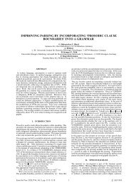
Fig. 1: Left: schematic view of a golf putt. Adapted from [1]. Right: gyroscope Y-axis data view. Swing phases: 1: backswing, 2: forward swing, 3: impact and 4: follow-through. 2.2. Mobile research platform Our putt coaching system built up on a research platform that we are using for mobile body area network applications. It consisted of SHIMMER sensor nodes [8] and an Android-based HTC Legend smartphone (HTC Corporation, Taoyuan, Taiwan). We used the gyroscope sensor module and the on-board accelerometer of the SHIMMER nodes in our study. Three-axis gyroscope data with a range of ±500 deg/s and three-axis accelerometer data with a range of ±1.5 g from a single sensor node mounted on top the golf club head was recorded with a frequency of 250 Hz and transmitted via Bluetooth radio. We implemented our coaching software engine on a HTC Legend smartphone that ran Android Version 2.1 on a MSM7227 microprocessor (600 MHz) with 512 MB main memory. The resulting app was based on a communication software that was developed within our research group [9]. 2.3. Data collection We collected data from eleven subjects (1 female, 10 male) that were either experienced golfers (n=5) or completely unexperienced (n=6). One participant was a professional golfer. After individually warming up, each subject performed five consecutive putts from three different distances labelled as short (1m), mid (3m) and long (5m) on an even training green at the Golf Club Herzogenaurach, Germany. The subjects were not restricted to any behaviour or technique. We recorded the whole sequence of putts including training swings without hitting the ball and arbitrary movements. Each subject started the experiment with the shortest distance and finished with the longest. The experiment was then repeated with a variation in either the golf club or the ball. We used two mallet type putters, the TaylorMade (TaylorMade Inc. Carlsbad, USA) Spider and the Pro Ace (Pro Ace Ltd., London, UK) 20704. As golf balls, the TaylorMade Noodle Longest and Burner LDP were used. The variation was arbitrarily chosen and delivered two data sets of 15 putts for each subject. Three blocks of five putts were missing due to sensor malfunction so that we recorded 315 putts overall. Each actual putt was marked in the data set by an external manual trigger for segmentation validation. 2.4. Preprocessing and initial segmentation The aim of this step was to extract stroke candidates and determine two major swing phases as defined in our swing model. As a preprocessing step, we applied a low-pass Butterworth filter of order 3 with a cut-off frequency of 8 Hz. The following two-step algorithm is based on the filtered data. First, we implemented a matched filter algorithm to roughly segment the signal in stroke candidates and other signals. In this approach, a template is correlated with a given signal to check for the presence of this template. Equation 1 shows the computation of the correlation value C for an M-dimensional signal x and the M-dimensional template b of length N. The factors α k scale each dimension for their contribution to the correlation value. The main movement axes of a golf putt contributed to the correlation in our algorithm. We calculated a template out of the ten short distance strokes of the professional golfer and reversed the resulting template to align the signals for the above-mentioned computation. The scaling factors were used to adjust the different value ranges of the axes. The € resulting C value was used together with an empirical threshold that was set by observation to identify a set of stroke candidates. € C = M N ∑α k k =1 i=1 ∑ x( t − i)⋅ b( i) (1) Second, we determined the major swing phases in these candidates. They were the backswing (BS) phase on the one hand and the combined forward swing (FS), impact (IP) and follow-through (FT) phase on the
other hand. The instants of time that border these two phases were zero-crossings in the gyroscope y-axis data (Fig. 1, right). 2.5. False stroke elimination and stroke segmentation We eliminated false stroke detections based on the stroke candidates and their corresponding stroke phases from the previous step. We used a two-stage approach including a plausibility analysis of timing and rotation speed and an impact check. In a first step, the plausibility analysis regarded the temporal ratio of BS to FS/IP/FT and the ratio of minimal backward to maximal forward rotation speed. The temporal ratio was based on typical putt timing from [1] while the rotation speed ratio was chosen to eliminate pendulum movements that violate our swing model. Strokes that did not fit in the predefined bounds were excluded from further analysis. In a second step, candidate strokes without a distinct high-frequency signal characterizing an impact event were excluded. In contrast to the previous segmentation stages, the unfiltered data was used. We created a characteristic pattern by analyzing the impact of all labelled FS/IP/FT phases. Our algorithm then searched the candidate stroke swing phases for this pattern. On absence of the pattern, the stroke was rejected from further analysis. Otherwise, the stroke was further segmented in forward swing, impact and followthrough. The impact duration was set to a constant value using typical stroke timing [1]. Table 1: Overview of features computed for each golf putt Number Description Number Description 1 Duration of BS 17 BS rotation angle 2 Duration of FS 18 FS rotation angle 3 Duration of BS and FS 19 FT rotation angle 4 Duration of FT 20 Ratio of FS rotation angle to FT rotation angle 5 Temporal ratio of FS to FT 21 Acceleration change in pre impact phase of accelerometer x-axis 6 Temporal ratio of BS to FS 22 Acceleration change in post impact phase of accelerometer x-axis 7 Duration of stroke 23 Rotation velocity of gyro y-axis at impact 8-10 Summed rotation in BS and FS phase of gyro x-, y- and z-axis 24 Horizontal velocity of accelerometer x-axis at impact 11-13 Summed rotation in pre impact phase of gyro x-, y- and z-axis 25-26 Acceleration maximum (x-axis) in FS (position, value) 14-16 Summed rotation in post impact phase of gyro x-, y- and z-axis 27-28 Velocity maximum (x-axis) in FS (position, value) 2.6. Feature extraction The coaching feedback we provided is based on putt parameters. Our literature research revealed various parameters that characterize correct putts and also describe kinematic findings that distinguish expert from novice players. We built a set of 28 features (Tab. 1) that were computed for each putt. We defined the preand post-impact phases as ¼ of the forward swing and the follow-through, respectively. 2.7. Coaching advices and putt score We gathered a set of eight coaching advices as putt feedback. Therefore, we analyzed the distribution of different parameter values and combined these findings with expert knowledge and our stroke model assumptions. See Tab. 2 for an overview. Beside the textual feedback, we introduced an overall putt score based on the coaching advice computation. Perfect fulfilment of an aspect results in two points and partial completion in one point. 16 points could be reached for a stroke in total. 2.8. Implementation The presented algorithms were implemented in a Matlab(The Mathwork Inc., Natick, USA) prototype. They served as the basis for porting the algorithms to Java software running on the device described above. 3. Results The developed segmentation algorithm reached a false detection rate of 1%. The misdetections appeared in the shortest distance experiment parts. These patterns were manually excluded from further analysis. All stroke phases were recognized correctly according to our stroke model. We analyzed the mean score for the two population groups for all distances. The mean score was 13.4 (± 2.4) for the experienced golfers and 11.4 (± 2.4) for the unexperienced subjects. The professional golfer reached the full score for every putt performed. The Android app proved to run on the target device. The device displayed the coaching advices, the score, the backswing rotation angle and the horizontal impact speed of a detected putt.
Page 1: Sensor-based Instant Golf Putt Feed

Sensor-based Instant Golf Putt Feedback

You also want an ePaper? Increase the reach of your titles

Delete template?

Save as template?