Error Estimation of SPECT OSEM with 3D Resolution Recovery ...

2008 IEEE Nuclear Science Symposium Conference Record M06-305
Towards Quantitative SPECT: Error Estimation of
SPECT OSEM with 3D Resolution Recovery,
Attenuation Correction and Scatter Correction
J. Zeintl, Student Member, IEEE, A. H. Vija, Member, IEEE, A. Yahil, Member, IEEE, X. Ding, Member, IEEE, J.
Hornegger, Member, IEEE, and T. Kuwert
Abstract– In this study we systematically investigate biases
relevant to quantitative SPECT if OSEM with isotropic (3D)
depth dependent resolution recovery (OSEM-3D), attenuation
and scatter correction is used. We focus on the dependencies of
activity estimation errors on the projection operator, structure
size, pixel size, count density and reconstruction parameters. We
use Tc-99m to establish a base line. Four Siemens low energy
collimators (Low Energy Ultra High Resolution, Low Energy
High Resolution, Low Energy All Purpose, Low Energy High
Sensitivity) with geometric resolution between 4.4 mm and 13.1
mm at 10 cm distance and sensitivity between 100 cpm/μCi and
1020 cpm/μCi are tested with simulations of spheres with
diameters between 9.8 mm and 168 mm in background. Pixel
sizes and total counts are varied between 2.4 mm and 9.6 mm and
0.125 and 32 million counts. Images are reconstructed with
OSEM-3D (Flash3D) with attenuation and scatter correction.
Emission recovery is quantitatively measured for different
reconstruction parameter settings. In addition, physical
measurements of standard quality control phantoms are
performed using an actual SPECT/CT system (Symbia® T6).
Cross calibration of the imaging system with a well counter and
results from simulations are used to quantitatively estimate the
true activity concentration in the physical phantoms. Results
show variations of emission recovery between 13.8% and 104.5%
depending on sphere volume and number of OSEM-3D updates.
After correction for the emission recovery errors and cross
calibration of the imaging system the errors in absolute
quantitation using the physical sphere phantom are between
+0.01±0.61% for the largest (16 ml) and -5.87±1.00% for the
smallest (0.5 ml) sphere. As a conclusion, the emission recovery
varies over a wide range and is highly dependent on imaging
parameters when using OSEM-3D reconstruction. Accurate
quantitation in phantoms is possible given that errors at the
specific imaging operation point can be estimated. In a clinical
setup this is a nontrivial task, and perhaps too cumbersome for
routine clinical use.
Manuscript received November 14, 2008. Asterisk indicates corresponding
author.
*Johannes Zeintl is a PhD student with the University of Erlangen-
Nuremberg, Institute of Pattern Recognition, Erlangen, Germany. (e-mail:
Johannes.Zeintl@uk-erlangen.de).
A. Hans Vija, Ding Xinhong are with Siemens Medical Solution USA,
Inc., Molecular Imaging, Hoffman Estates, IL 60192, USA.
Amos Yahil is with Image Recon LLC, Stony Brook, NY, USA.
Joachim Hornegger is with the University of Erlangen-Nuremberg,
Institute of Pattern Recognition, Erlangen, Germany.
Torsten Kuwert is with the University of Erlangen-Nuremberg, Clinic of
Nuclear Medicine.
I. INTRODUCTION
N clinical SPECT imaging iterative reconstruction
Itechniques are now a common alternative to filtered
backprojection [5]. Ordered subset expectation
maximization (OSEM) is often the iterative method of choice
([3], 10]). The advantage of iterative methods is the ability to
correct for image degradations introduced by imaging physics
such as depth dependent blur, photon attenuation, and scatter.
It was shown that these corrections minimize errors for
absolute quantitation in SPECT imaging ([2], [9], [11], [12]).
Active research is conducted to improve correction techniques
for quantitation in SPECT ([16] – [20]) and to evaluate
common reconstruction methods and establish practical
baselines ([4], [6], [13], [15]). However, less attention was
paid to the non-stationary behavior of OSEM in terms of
quantitation and the dependency of quantitation errors on
imaging parameters. In this work we systematically
investigate biases relevant to quantitative SPECT if OSEM
with isotropic (3D) depth dependent resolution recovery
(OSEM-3D), attenuation and scatter correction is used. We
focus on the dependencies of activity estimation errors on the
projection operator, structure size, pixel size, count density,
and reconstruction parameters. We use the obtained results to
correct for the non-stationarity of OSEM in physical phantom
experiments performed on a cross-calibrated SPECT/CT
system.
II. MATERIAL AND METHODS
Three steps were performed to derive absolute values for
activity concentrations from reconstructed images of actual
measured data:
A: Estimation of emission recovery errors for various
imaging parameter sets using simulations.
B: Cross calibration of the SPECT/CT imaging system with
the well counter.
C: Appliance of correction factors derived from A and B to
measured phantom data.
978-1-4244-2715-4/08/$25.00 ©2008 IEEE
4106

A. Simulations of imaging system
Quasi-analytical simulations (voxel size: 0.6 mm) are
performed by modeling the projection operator in 3D
according to the detector and collimator specifications of the
Siemens Symbia T-series gamma cameras with the parameters
listed in Table I, and assuming a perfect collimator. Poisson
noise is added to the generated projection data. Photon
attenuation in the object is accounted for and a derived μ-map
is used for attenuation correction. We assume an acquisition
with perfect scatter rejection of 140keV (Tc-99m) photons.
for a given object j at a given imaging parameter set i. The
boundaries of the target object to be measured are derived
from the true high resolution image (Fig. 1 top row). Partial
volume effects, specifically spill-in and spill-out at the object
boundaries due to finite pixel size, are compensated for by
measuring the loss of emission in the simulation using
different pixel sizes.
B. Cross Calibration of the Imaging System
TABLE I
COLLIMATOR SPECIFICATIONS OF FOUR SIEMENS LOW ENERGY COLLIMATORS
Acceptance
Angle (rad)
Sensitivity
(cpm/μCi)
Hole Length
(mm)
Geometric
Resolution @
10cm (mm)
LEHS 0.115194 1020 24.05 13.4
LEAP 0.064973 330 24.05 7.6
LEHR 0.049514 202 24.05 5.9
LEUHR 0.034632 100 35.8 4.4
LEHS: Low Energy High Sensitivity, LEAP: Low Energy All Purpose, LEHR:
Low Energy High Resolution, LEUHR: Low Energy Ultra High Resolution
Hot spheres with diameters between 9.8 mm and 168 mm in a
warm cylindrical background (Sphere to background ratio
10:1) are simulated. Pixel size and total counts are varied
between 2.4 mm and 9.6 mm and 0.125 and 32 million counts.
Image reconstruction is performed using MLEM/OSEM with
isotropic resolution recovery (Flash3D) and attenuation
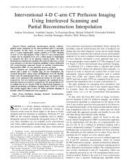
correction. Fig. 1 shows example images of simulated and
reconstructed spheres.
Fig. 1: True (top row) and example reconstructed images (bottom row, LEHR
collimation, 2.4 mm voxel, 32 OSEM updates) of the simulated spheres of
different diameters in a 10% background.
Images are analyzed in terms of emission recovery. The
emission recovery coefficient is defined as:
( j i)
( j)
Measured Emission ,
C E
( j, i)
= , (1)
True Emission
Fig. 2: Acquisition setup for the cross calibration of the imaging system. A
large cylindrical phantom is filled uniformly with a known activity
concentration derived from a well counter and acquired in the SPECT/CT
imaging system.
The cross calibration of the SPECT/CT system is done
using a large cylindrical phantom uniformly filled with water
and a known activity concentration of Tc-99m measured in a
well counter (see Fig. 2). 50 million total counts are collected
in a 360 degree acquisition range, 120 projections, and a 150
mm detector radius from the center of rotation. A dual energy
window was used for the acquisition of the photo peak and the
lower scatter (15% window width, respectively). An
attenuation map was generated from a CT scan of the
phantom. Data are reconstructed using OSEM with isotropic
beam modeling (Flash3D) and scatter and attenuation
correction.
To calculate the system volume sensitivity a large volume
of interest (> 3000 ml) is drawn and the count rate per volume
is derived. The decay corrected count rate is calculated as
follows:
ˆ
⎛ T − T ⎞ ⎛
0 ln 2 ⎞⎛
⎛ ⎞⎞
exp ln 2 ⎜1
exp ln 2 ⎟
×
t
R = R ×
⎜ ⎟
⎜
⎟
−
⎜ −
⎟ (2)
⎝ T1/
2 ⎠ ⎝ T1/
2 ⎠⎝
⎝ T1/
2 ⎠⎠
Where R is the count rate derived from the reconstructed
image, T is the start time of the acquisition, T 0 is the time of
the activity calibration, T 1/2 is the half time of the isotope, and
t is the time duration of the acquisition.
The system volume sensitivity is then:
−1
4107

S
Rˆ
/ t
Dwell
Vol
= (3)
cA
Where t Dwell is the total dwell time of the acquisition (t Dwell =
t in continuous acquisition mode) and c A is the actual activity
concentration in the phantom measured by the well counter.
C. Appliance of corrections on real phantom data
To evaluate the quantitative accuracy of the SPECT/CT
imaging system a standard quality control sphere phantom
(Data Spectrum, Hillsborough, NC) is acquired. The activity
concentration is 19.6 μCi/ml (725 kBq/ml) in the spheres and
1.7 μCi/ml (63 kBq/ml) in the background, resulting in a
concentration ratio of approx. 12:1. The phantom is acquired
in the center of the field of view using a 150 mm detector
radius of rotation over a 360° scan range. LEHR collimation is
used with a 2.4 mm pixel size. The total number of counts is
24 million.
The data are reconstructed with Flash3D with scatter and
CT based attenuation correction. Volumes of interest are
drawn manually using the CT boundaries of the fused
SPECT/CT image (see Fig. 3). The absolute activity
concentration for a given object size j is calculated by
( j)
/ t
Dwell
C ( j,
i′
)
RVOI
cˆ A
( j)
=
, (4)
S
Vol
where R VOI is the count rate per volume in the drawn
volume of interest and i’ the specific imaging parameter set
used.
E
Fig. 3: Reconstructed image of the sphere phantom fused with the CT image
(LEHR collimation, 2.4 mm voxel, 32 OSEM updates). Volumes of interest
were drawn manually using the CT boundaries.
III. RESULTS
A. Simulation Results
In Fig. 4 the loss of emission recovery due to spill over at
the object boundaries is shown for the different object and
voxel sizes used. The values are derived from the simulation
tool when a target to background ratio of 10:1 is used. In
subsequent results these values are applied as a postprocessing
step after reconstruction to compensate for the
effect by adding the respective value to the emission recovery
coefficients measured in the simulations.
Measured Emission Recovery in Object
120%
100%
80%
60%
40%
20%
0%
0 30 60 90 120 150
Sphere Diameter (mm)
2.4 mm voxel
4.8 mm voxel
9.6 mm voxel
Fig. 4: The effect of spill over at object boundaries on emission recovery due
to finite voxel size for different object and voxel sizes (target to background
ratio is 10:1).
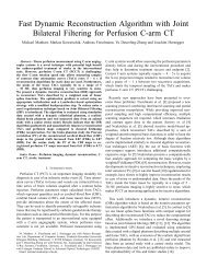
Fig. 5 gives an overview of the emission recovery
coefficients for different object sizes, number of OSEM
updates, and voxel sizes used. Results are shown for LEHR
collimation and 2 million total counts. For small object and
voxel sizes (2.4 mm, 4.8 mm) the over shooting characteristic
of OSEM at high numbers of updates is visible. In general the
emission recovery coefficient is highly dependent on the
number of OSEM updates especially for object sizes below 3
times the system resolution. This dependency at small object
sizes is more pronounced for finer data sampling (smaller
voxels).
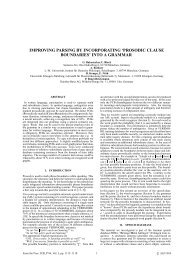
The dependency of emission recovery on the projection
operator is shown in Fig. 6. The recovery coefficient for
LEUHR, LEAP, and LEHS collimation is shown using 2.4
mm voxel size, and 1 million, 4.5 million, and 10 million total
counts for LEUHR, LEAP, and LEHS collimation,
respectively. At small object sizes the effect of the beam
geometry on the emission recovery is noticeable and results in
lower values for broader beam collimators.
4108

Recovery Coefficient
Recovery Coefficient
Recovery Coefficient
1.2
1
0.8
0.6
0.4
0.2
LEHR 2.4 mm Voxel Size
0
0 5 10 15
1.2
1
0.8
Sphere Diameter (mm)
0 30 60 90 120 150
Sphere Diameter (mm) / System Resolution (mm)
LEHR 4.8 mm Voxel Size
128 upds
64 upds
32 upds
16 upds
8 upds
4 upds
0.6
128 upds
64 upds
0.4
32 upds
16 upds
0.2
8 upds
4 upds
0
0 5 10 15
1.2
1
0.8
0.6
0.4
0.2
0
Sphere Diameter (mm)
0 30 60 90 120 150
Sphere Diameter (mm) / System Resolution (mm)
LEHR 9.6 mm Voxel Size
Sphere Diameter (mm)
0 30 60 90 120 150
128 upds
64 upds
32 upds
16 upds
8 upds
4 upds
0 5 10 15
Sphere Diameter (mm) / System Resolution (mm)
Fig. 5: Emission recovery coefficients for different object sizes, number of
OSEM updates, and voxel sizes using LEHR collimation and 2 million total
counts. Values are corrected for spill over effects at the object boundaries
using results of Fig. 4. Each data point is obtained using the average value of
5 independent realizations.
Recovery Coefficient
Recovery Coefficient
Recovery Coefficient
1.2
1
0.8
0.6
0.4
0.2
1.2
1
0.8
0.6
0.4
0.2
LEUHR 2.4 mm Voxel Size
Sphere Diameter (mm)
0 30 60 90 120 150
0
0 5 10 15 20
1.2
1
0.8
0.6
0.4
0.2
Sphere Diameter (mm) / System Resolution (mm)
LEAP 2.4 mm Voxel Size
0
0 5 10
LEHS 2.4 mm Voxel Size
128 upds
64 upds
32 upds
16 upds
8 upds
4 upds
Sphere Diameter (mm)
0 30 60 90 120 150
128 upds
64 upds
32 upds
16 upds
8 upds
4 upds
Sphere Diameter (mm) / System Resolution (mm)
Sphere Diameter (mm)
0 30 60 90 120 150
128 upds
64 upds
32 upds
16 upds
8 upds
4 upds
0
0 2 4 6 8
Sphere Diameter (mm) / System Resolution (mm)
Fig. 6: Emission recovery coefficients for different object sizes, number of
OSEM updates, and collimation schemes using 2.4 mm voxels and 1 million,
4.5 million, and 10 million total counts for LEUHR, LEAP, and LEHS
collimation, respectively. Values are corrected for spill over effects at the
object boundaries using results of Fig. 4. Each data point is obtained using the
average value of 5 independent realizations.
4109

The dependency of total counts on the emission recovery is
shown in Fig. 7. Beyond 3 times the system resolution the
standard deviation of the recovery coefficient is below 0.0035
for all count levels tested. Below this point standard deviations
are between 0.0056 and 0.0233 for 16ml and 0.5ml spheres,
respectively.
Recovery Coefficient
1.2
1.1
1
0.9
0.8
0.7
0.6
0.5
Sphere Diameter (mm)
0 30 60 90 120 150
0.125 Mcts
0.500 Mcts
1 Mcts
2 Mcts
4 Mcts
16 Mcts
32 Mcts
0.4
0 5 10 15
Sphere Diameter (mm) / System Resolution (mm)
Fig. 7: Emission recovery coefficients for different total count levels using
LEHR collimation, 2.4 mm voxel size and 32 OSEM updates. Each data point
is obtained using the average value of 5 independent realizations.
B. Quantitative Results from Phantom Experiment
Using the simulated recovery coefficient for the specific
operation point of the phantom experiment (Section II C)
which is between 0.485 and 0.898 for the smallest and the
largest sphere respectively and applying Equation 4, the
absolute activity concentrations are calculated for all 6
spheres. The results are summarized in Table II showing
absolute quantification errors between -5.87% and 0.01% for
the smallest and largest sphere, respectively.
Reference Values*
Sphere
Volume
(ml)
TABLE II
RESULTS FROM PHANTOM EXPERIMENT
Activity
Concentratio
n (μCi/ml)
VOI Mean
Volume
(ml)
Image Based
Calculated
Mean
Activity
Concentratio
n (μCi/ml)
Activity
Concentratio
n Standard
Deviation**
(μCi/ml)
Difference -
Reference
vs.
Calculated
(%)
16 16.3 19.59 0.12 -0.01 ± 0.61
8 8.2 20.03 0.13 +2.25 ± 0.66
4 4.1 20.11 0.29 +2.62 ± 1.48
19.6
2 2.0 19.60 0.22 +0.02 ± 1.15
1 1.1 18.65 0.34 -4.81 ± 1.73
0.5 0.6 18.44 0.19 -5.87 ± 1.00
*according to manufacturer specifications and well counter measurements
**manual determination of VOIs by 2 operators, 2 repeats each
IV. DISCUSSION
The object evaluated in the phantom experiment
geometrically correlates well to the objects in the simulation,
i.e. object sizes and positions are similar. In addition, the
scanner geometry including e.g. detector orbit and radius, of
simulation and experiment is kept identical. Thus,
dependencies of geometric conditions on the emission
recovery are disregarded.
The method used to simulate the imaging system only takes
the primary photons of 140 keV into account, neglecting both
septal penetration as well as object and collimator scattering.
These effects are present in the real data even though
corrected using the standard techniques provided by the
reconstruction software package. These inconsistencies might
introduce errors.
During the cross calibration step for obtaining the system
volume sensitivity additional errors are introduced due to both
systematic and statistical errors of physical volume and
activity measurements.
In the phantom experiment the object boundaries are drawn
manually resulting in variable size and shape even though
fused CT data is used. To create reproducible results and for
use in clinical workflows automatic or semi automatic
segmentation tools are preferable.
The developed procedure shows promising results for
absolute quantitation in SPECT. However, a careful analysis
incorporating all the various sources of error is required, in
order to make this procedure more universally valid.
V. CONCLUSION
Results from simulations show that the emission recovery
varies over a wide range and is highly dependent on imaging
parameters when using OSEM-3D reconstruction. Highest
variations are in the clinical relevant domain below three times
the imaging system resolution. Accurate quantitation in
phantoms is possible given that errors at the specific imaging
operation point can be estimated. In a clinical setup this is a
nontrivial task, and perhaps too cumbersome for routine
clinical use.
ACKNOWLEDGMENTS
The authors would like to thank Ron Malmin and Manjit
Ray for valuable discussions and the Systems Test team at
Hoffman Estates for their help during system quality control
and acquisition of the data.
REFERENCES
[1] H. H. Barrett, and e. al., “Noise Properties of the EM algorithm: I.
Theory,” Physics in Medicine and Biology, vol. 39, pp. 833-846, 1994.
[2] D. R. Gilland, R. J. Jaszczak, J. E. Bowsher et al., “Quantitative SPECT
Brain Imaging: Effects of Attenuation and Detector Response,” Nuclear
Science, IEEE Transactions on, vol. 40, no. 3, pp. 295-299, 1993.
[3] H. M. Hudson, and R. S. Larkin, “Accelerated Image Reconstruction
using Ordered Subsets of Projection Data,” Medical Imaging, IEEE
Transactions on, pp. 100-108, 1994.
[4] C. Kamphuis, F. J. Beekman, and M. A. Viergever, “Evaluation of OS-
EM vs. ML-EM for 1D, 2D and fully 3D SPECT reconstruction,”
4110

Nuclear Science, IEEE Transactions on, vol. 43, no. 3, pp. 2018-2024,
1996.
[5] F. C. Klocke, and e. al., “ACC/AHA/ASNC Guidelines for the Clinical
Use of Cardiac Radionuclide Imaging,” ACC/AHA/ASNC Practice
Guidelines, 2003.
[6] T. R. Miller, and J. W. Wallis, “Clinically Important Characteristics of
Maximum-Likelihood Reconstruction,” Journal of Nuclear Medicine,
vol. 33, pp. 1678-1684, 1992.
[7] J. Nuyts, “On Estimating the Variance of Smoothed MLEM Images,”
Nuclear Science, IEEE Transactions on, vol. 49, no. 3, pp. 714-721,
2002.
[8] P. H. Pretorius, M. A. King, T.-S. Pan et al., “Reducing the influence of
the partial volume effect on SPECT activity quantitation with 3D
modelling of spatial resolution in iterative reconstruction,” Physics in
Medicine and Biology, vol. 43, pp. 407-420, 1998.
[9] M. S. Rosenthal, J. Cullom, W. Hawkins et al., “Quantitative SPECT
Imaging: A Review and Recommendations by the Focus Commitee of
the Society of Nuclear Medicine Computer and Instrumentation
Council,” Journal of Nuclear Medicine, vol. 36, pp. 1489-1513, 1995.
[10] L. A. Shepp, and Y. Vardi, “Maximum Likelihood Reconstruction for
Emission Tomography,” Medical Imaging, IEEE Transactions on, vol.
MI-1, no. 2, pp. 113-122, 1982.
[11] B. M. W. Tsui, E. C. Frey, X. Zhao et al., “The importance and
implementation of accurate 3D compensation methods for quantitative
SPECT,” Physics in Medicine and Biology, vol. 39, pp. 509-530, 1994.
[12] B. M. W. Tsui, X. Zhao, E. C. Frey et al., “Quantitative Single-Photon
Emission Computed Tomography: Basics and Clinical Considerations,”
Seminars in Nuclear Medicine, vol. 14, no. 1, pp. 38-65, 1994.
[13] A. H. Vija, E. G. Hawman, and J. C. Engdahl, “Analysis of a SPECT
OSEM Reconstruction Method with 3D Beam Modeling and Optional
Attenuation Correction: Phantom Studies,” IEEE NSS/MIC Conference
Record, 2003.
[14] D. W. Wilson, and H. H. Barrett, “The Effects of Incorrect Modeling on
Noise and Resolution Properties of ML-EM Images,” Nuclear Science,
IEEE Transactions on, vol. 49, no. 3, pp. 768-773, 2002.
[15] T. Yokoi, and e. al., “Performance Evaluation of OSEM reconstruction
algorithm incorporating three-dimensional distance-dependent resolution
compensation for brain SPECT: A simulation study,” Annuals of
Nuclear Medicine, vol. 16, no. 1, pp. 11-18, 2002.
[16] S. Shcherbinin and A. Celler, “An investigation of iterative
reconstructions in quantitative SPECT”, Journal of Physics: Conference
Series 124 (2008)
[17] S. Shcherbinin and A. Celler, “Non-iterative quantitative SPECT
reconstructions with a reduced size system matrix”, 2007 IEEE Nuclear
Science Symposium Conference Record, M13-325
[18] E. Vandervoort, A. Celler, and R. Harrop, “Implementation of an
iterative scatter correction, the influence of attenuation map quality and
their effect on absolute quantitation in SPECT”, Phys. Med. Biol. 52
(2007), 1527-1545
[19] S. Liu and T.H. Farncombe, “Collimator-Detector Response
Compensation in Quantitative SPECT Reconstruction”, 2007 IEEE
Nuclear Science Symposium Conference Record, M19-327
[20] K. Willowson, et al., “Quantitative SPECT reconstruction using CTderived
corrections”, Phys. Med. Biol. 53 (2008), 3099-3112
4111