PSTricks pst-plot plotting data and functions
PSTricks pst-plot plotting data and functions
PSTricks pst-plot plotting data and functions
- No tags were found...

Create successful ePaper yourself
Turn your PDF publications into a flip-book with our unique Google optimized e-Paper software.
<strong>PSTricks</strong><br />
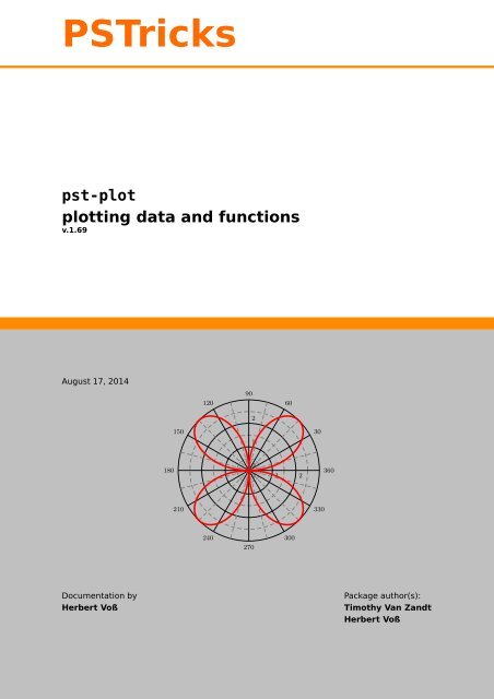
<strong>pst</strong>-<strong>plot</strong><br />
<strong>plot</strong>ting <strong>data</strong> <strong>and</strong> <strong>functions</strong><br />
v.1.69<br />
August17,2014<br />
120<br />
90<br />
2<br />
60<br />
150<br />
1<br />
30<br />
180<br />
0<br />
0<br />
1<br />
2<br />
360<br />
210<br />
330<br />
240<br />
270<br />
300<br />
Documentationby<br />
Herbert Voß<br />
Package author(s):<br />
Timothy Van Z<strong>and</strong>t<br />
Herbert Voß
2<br />
This version of <strong>pst</strong>-<strong>plot</strong> uses the extended keyval h<strong>and</strong>ling of <strong>pst</strong>-xkey<br />
<strong>and</strong>hasalotofthemacroswhichwererecentlyinthepackage<strong>pst</strong>ricks-add.<br />
This documentation describes only the new <strong>and</strong> changed stuff. For the default<br />
behaviour look into the documentation part of the base <strong>pst</strong>ricks package.<br />
Youfindthedocumentationhere: http://mirrors.ctan.org/graphics/<br />
<strong>pst</strong>ricks/base/doc/.<br />
Thanks to: Guillaume van Baalen; Stefano Baroni; Martin Chicoine; Gerry<br />
Coombes; Ulrich Dirr; Christophe Fourey; Hubert Gäßlein; Jürgen Gilg; Denis<br />
Girou; Peter Hutnick; Christophe Jorssen; Uwe Kern; Alex<strong>and</strong>er Kornrumpf;<br />
Manuel Luque; Patrice Mégret; Jens-Uwe Morawski; Tobias Nähring;<br />
RolfNiepraschk;MartinPaech;AlanRistow;ChristineRömer;ArnaudSchmittbuhl
Contents 3<br />
Contents<br />
I. Basic comm<strong>and</strong>s, connections <strong>and</strong> labels 5<br />
1. Introduction 5<br />
2. Plotting <strong>data</strong> records 5<br />
3. Plotting mathematical <strong>functions</strong> 7<br />
II. New comm<strong>and</strong>s 8<br />
4. Extended syntax 8<br />
5. New Macro \psBox<strong>plot</strong> 10<br />
6. The psgraph environment 15<br />
6.1. Coordinates of the psgraph area . . . . . . . . . . . . . . . . . . . . . . . . 21<br />
6.2. The new options for psgraph . . . . . . . . . . . . . . . . . . . . . . . . . . 21<br />
6.3. The new macro \pslegend for psgraph . . . . . . . . . . . . . . . . . . . . 22<br />
7. \psxTick <strong>and</strong> \psyTick 25<br />
8. \<strong>pst</strong>ScalePoints 25<br />
9. New or extended options 26<br />
9.1. Introduction . . . . . . . . . . . . . . . . . . . . . . . . . . . . . . . . . . . 26<br />
9.2. Option <strong>plot</strong>style (Christoph Bersch) . . . . . . . . . . . . . . . . . . . . . 28<br />
9.3. Option xLabels, yLabels, xLabelsrot, <strong>and</strong> yLabelsrot . . . . . . . . . . 29<br />
9.4. Option xLabelOffset <strong>and</strong> ylabelOffset . . . . . . . . . . . . . . . . . . . 29<br />
9.5. Option yMaxValue <strong>and</strong> yMinValue . . . . . . . . . . . . . . . . . . . . . . . 30<br />
9.6. Option axesstyle . . . . . . . . . . . . . . . . . . . . . . . . . . . . . . . . 32<br />
9.7. Option xyAxes, xAxis <strong>and</strong> yAxis . . . . . . . . . . . . . . . . . . . . . . . . 34<br />
9.8. Option labels . . . . . . . . . . . . . . . . . . . . . . . . . . . . . . . . . . 34<br />
9.9. Options xlabelPos <strong>and</strong> ylabelPos . . . . . . . . . . . . . . . . . . . . . . . 35<br />
9.10. Options x|ylabelFontSize <strong>and</strong> x|ymathLabel . . . . . . . . . . . . . . . . 36<br />
9.11. Options xlabelFactor <strong>and</strong> ylabelFactor . . . . . . . . . . . . . . . . . . 37<br />
9.12. Options decimalSeparator <strong>and</strong> comma . . . . . . . . . . . . . . . . . . . . 38<br />
9.13. Options xyDecimals, xDecimals <strong>and</strong> yDecimals . . . . . . . . . . . . . . . 39<br />
9.14. Option triglabels . . . . . . . . . . . . . . . . . . . . . . . . . . . . . . . 39<br />
9.15. Option ticks . . . . . . . . . . . . . . . . . . . . . . . . . . . . . . . . . . . 47<br />
9.16. Option tickstyle . . . . . . . . . . . . . . . . . . . . . . . . . . . . . . . . 48<br />
9.17. Options ticksize, xticksize, yticksize . . . . . . . . . . . . . . . . . . 48<br />
9.18. Options subticks, xsubticks, <strong>and</strong> ysubticks . . . . . . . . . . . . . . . . 50<br />
9.19. Options subticksize, xsubticksize, ysubticksize . . . . . . . . . . . . 50<br />
9.20. tickcolor <strong>and</strong> subtickcolor . . . . . . . . . . . . . . . . . . . . . . . . . 51
Contents 4<br />
9.21. ticklinestyle <strong>and</strong> subticklinestyle . . . . . . . . . . . . . . . . . . . . 52<br />
9.22. logLines . . . . . . . . . . . . . . . . . . . . . . . . . . . . . . . . . . . . . 52<br />
9.23. xylogBase, xlogBase <strong>and</strong> ylogBase . . . . . . . . . . . . . . . . . . . . . . 54<br />
9.24. xylogBase . . . . . . . . . . . . . . . . . . . . . . . . . . . . . . . . . . . . 54<br />
9.25. ylogBase . . . . . . . . . . . . . . . . . . . . . . . . . . . . . . . . . . . . . 55<br />
9.26. xlogBase . . . . . . . . . . . . . . . . . . . . . . . . . . . . . . . . . . . . . 57<br />
9.27. No logstyle (xylogBase={}) . . . . . . . . . . . . . . . . . . . . . . . . . . . 58<br />
9.28. Option tickwidth <strong>and</strong> subtickwidth . . . . . . . . . . . . . . . . . . . . . 59<br />
9.29. Option psgrid, gridcoor, <strong>and</strong> gridpara . . . . . . . . . . . . . . . . . . . 63<br />
10.New options for \read<strong>data</strong> 64<br />
11.New options for \list<strong>plot</strong> 65<br />
11.1. Options nStep, xStep, <strong>and</strong> yStep . . . . . . . . . . . . . . . . . . . . . . . 65<br />
11.2. Options nStart <strong>and</strong> xStart . . . . . . . . . . . . . . . . . . . . . . . . . . . 67<br />
11.3. Options nEnd <strong>and</strong> xEnd . . . . . . . . . . . . . . . . . . . . . . . . . . . . . 68<br />
11.4. Options yStart <strong>and</strong> yEnd . . . . . . . . . . . . . . . . . . . . . . . . . . . . 69<br />
11.5. Options <strong>plot</strong>No, <strong>plot</strong>NoX, <strong>and</strong> <strong>plot</strong>NoMax . . . . . . . . . . . . . . . . . . . 69<br />
11.6. Option changeOrder . . . . . . . . . . . . . . . . . . . . . . . . . . . . . . . 72<br />
12.New <strong>plot</strong> styles 73<br />
12.1. Plot style colordot <strong>and</strong> option Hue . . . . . . . . . . . . . . . . . . . . . . 73<br />
12.2. Plot style bar <strong>and</strong> option barwidth . . . . . . . . . . . . . . . . . . . . . . 74<br />
12.3. Plot style ybar . . . . . . . . . . . . . . . . . . . . . . . . . . . . . . . . . . 76<br />
12.4. Plotstyle LSM . . . . . . . . . . . . . . . . . . . . . . . . . . . . . . . . . . . 77<br />
12.5. Plotstyles values <strong>and</strong> values* . . . . . . . . . . . . . . . . . . . . . . . . . 80<br />
12.6. Plotstyles xvalues <strong>and</strong> xvalues* . . . . . . . . . . . . . . . . . . . . . . . 81<br />
13.Polar <strong>plot</strong>s 82<br />
14.New macros 85<br />
14.1. \psCoordinates . . . . . . . . . . . . . . . . . . . . . . . . . . . . . . . . . 85<br />
14.2. \psFixpoint . . . . . . . . . . . . . . . . . . . . . . . . . . . . . . . . . . . 86<br />
14.3. \psNewton . . . . . . . . . . . . . . . . . . . . . . . . . . . . . . . . . . . . 87<br />
14.4. \psVectorfield . . . . . . . . . . . . . . . . . . . . . . . . . . . . . . . . . 89<br />
15.Internals 90<br />
16.List of all optional arguments for <strong>pst</strong>-<strong>plot</strong> 91<br />
References 93
5<br />
Part I.<br />
Basic comm<strong>and</strong>s, connections <strong>and</strong><br />
labels<br />
1. Introduction<br />
The <strong>plot</strong>ting comm<strong>and</strong>s described in this part are defined in the very first version of<br />
<strong>pst</strong>-<strong>plot</strong>.tex <strong>and</strong> available for all new <strong>and</strong> ancient versions.<br />
The \psdots, \psline, \pspolygon, \pscurve, \psecurve <strong>and</strong> \psccurve graphics<br />
objects let you <strong>plot</strong> <strong>data</strong> in a variety of ways. However, first you have to generate the<br />
<strong>data</strong> <strong>and</strong> enter it as coordinate pairs x,y. The <strong>plot</strong>ting macros in this section give you<br />
other ways to get <strong>and</strong> use the <strong>data</strong>.<br />
To parameter <strong>plot</strong>style=style determines what kind of <strong>plot</strong> you get. Valid styles<br />
aredots,line,polygon, curve,ecurve,ccurve. E,g.,ifthe<strong>plot</strong>style ispolygon, then<br />
the macro becomes a variant of the \pspolygon object.<br />
You can use arrows with the <strong>plot</strong> styles that are open curves, but there is no optional<br />
argument for specifying the arrows. You have to use the arrows parameter instead.<br />
No PostScript error checking is provided for the <strong>data</strong> arguments. There are systemdependent<br />
limits on the amount of <strong>data</strong> T E X <strong>and</strong> PostScript can h<strong>and</strong>le. You are much<br />
less likely to exceed the PostScript limits when you use the line, polygon or dots <strong>plot</strong><br />
style, with showpoints=false, linearc=0pt, <strong>and</strong> no arrows.<br />
Note that the lists of <strong>data</strong> generated or used by the <strong>plot</strong> comm<strong>and</strong>s cannot contain<br />
units. The values of \psxunit <strong>and</strong> \psyunit are used as the unit.<br />
<br />
2. Plotting <strong>data</strong> records<br />
\file<strong>plot</strong> [Options] {file}<br />
\psfile<strong>plot</strong> [Options] {file}<br />
\<strong>data</strong><strong>plot</strong> [Options] {\〈macro〉}<br />
\ps<strong>data</strong><strong>plot</strong> [Options] {\〈macro〉}<br />
\save<strong>data</strong>{\〈macro〉}[<strong>data</strong>]<br />
\read<strong>data</strong>{\〈macro〉}{file}<br />
\psreadColumnData{colNo}{delimiter}{\〈macro〉}{filename}<br />
\list<strong>plot</strong>{<strong>data</strong>}<br />
\pslist<strong>plot</strong>{<strong>data</strong>}<br />
The macros with a preceeding ps are equivalent to those without.<br />
\file<strong>plot</strong> is the simplest of the <strong>plot</strong>ting <strong>functions</strong> to use. You just need a file that<br />
containsalistofcoordinates(withoutunits),suchasgeneratedbyMathematicaorother<br />
mathematical packages. The <strong>data</strong> can be delimited by curly braces { }, parentheses<br />
( ), commas,<strong>and</strong>/or white space. Bracketing all the <strong>data</strong> with square brackets [ ] will<br />
significantlyspeeduptherateatwhichthe<strong>data</strong>isread,buttherearesystem-dependent
2. Plotting <strong>data</strong> records 6<br />
limits on how much <strong>data</strong> T E X can read like this in one chunk. (The [ must go at the<br />
beginning of a line.) The file should not contain anything else (not even \endinput),<br />
except for comments marked with %.<br />
\file<strong>plot</strong> only recognizes the line, polygon <strong>and</strong> dots <strong>plot</strong> styles, <strong>and</strong> it ignores<br />
the arrows, linearc <strong>and</strong> showpoints parameters. The \list<strong>plot</strong> comm<strong>and</strong>, described<br />
below, can also <strong>plot</strong> <strong>data</strong> from file, without these restrictions <strong>and</strong> with faster T E X processing.<br />
However, you are less likely to exceed PostScript’s memory or oper<strong>and</strong> stack<br />
limits with \file<strong>plot</strong>.<br />
IfyoufindthatittakesT E Xalongtimetoprocess your\file<strong>plot</strong> comm<strong>and</strong>,youmay<br />
want to use the \PSTtoEPS comm<strong>and</strong> described on page . This will also reduce T E X’s<br />
memory requirements.<br />
\<strong>data</strong><strong>plot</strong> is also for <strong>plot</strong>ting lists of <strong>data</strong> generated by other programs, but you first<br />
have to retrieve the <strong>data</strong> with one of the following comm<strong>and</strong>s: <strong>data</strong> or the <strong>data</strong> in file<br />
shouldconformtotherulesdescribed aboveforthe<strong>data</strong>in\file<strong>plot</strong> (with\save<strong>data</strong>,<br />
the <strong>data</strong> must be delimited by [ ], <strong>and</strong> with \read<strong>data</strong>, bracketing the <strong>data</strong> with [ ]<br />
speeds things up). You can concatenate <strong>and</strong> reuse lists, as in<br />
\read<strong>data</strong>{\foo}{foo.<strong>data</strong>}<br />
\read<strong>data</strong>{\bar}{bar.<strong>data</strong>}<br />
\<strong>data</strong><strong>plot</strong>{\foo\bar}<br />
\<strong>data</strong><strong>plot</strong>[origin={0,1}]{\bar}<br />
The \read<strong>data</strong> <strong>and</strong> \<strong>data</strong><strong>plot</strong> combination is faster than \file<strong>plot</strong> if you reuse the<br />
<strong>data</strong>. \file<strong>plot</strong> uses less of T E X’s memory than \read<strong>data</strong> <strong>and</strong> \<strong>data</strong><strong>plot</strong> if you are<br />
also use \PSTtoEPS.<br />
Here is a <strong>plot</strong> of ∫ sin(x)dx. The <strong>data</strong> was generated by Mathematica, with<br />
Table[{x,N[SinIntegral[x]]},{x,0,20}]<br />
<strong>and</strong> then copied to this document.<br />
<br />
<br />
<br />
\pspicture(4,3) \psset{xunit=.2cm,yunit=1.5cm}<br />
\save<strong>data</strong>{\my<strong>data</strong>}[<br />
{{0, 0}, {1., 0.946083}, {2., 1.60541}, {3., 1.84865}, {4., 1.7582},<br />
{5., 1.54993}, {6., 1.42469}, {7., 1.4546}, {8., 1.57419},<br />
{9., 1.66504}, {10., 1.65835}, {11., 1.57831}, {12., 1.50497},<br />
{13., 1.49936}, {14., 1.55621}, {15., 1.61819}, {16., 1.6313},<br />
{17., 1.59014}, {18., 1.53661}, {19., 1.51863}, {20., 1.54824}}]<br />
\<strong>data</strong><strong>plot</strong>[<strong>plot</strong>style=curve,showpoints,dotstyle=triangle]{\my<strong>data</strong>}<br />
\psline{}(0,2)(0,0)(22,0)<br />
\endpspicture<br />
\list<strong>plot</strong> is yet another way of <strong>plot</strong>ting lists of <strong>data</strong>. This time, should be a<br />
list of <strong>data</strong> (coordinate pairs), delimited only by white space. list is first exp<strong>and</strong>ed by
•<br />
•<br />
•<br />
•<br />
•<br />
•<br />
•<br />
•<br />
•<br />
3. Plotting mathematical<strong>functions</strong> 7<br />
T E X <strong>and</strong> then by PostScript. This means that list might be a PostScript program that<br />
leaves on the stack a list of <strong>data</strong>, but you can also include <strong>data</strong> that has been retrieved<br />
with \read<strong>data</strong> <strong>and</strong> \<strong>data</strong><strong>plot</strong>. However, when using the line, polygon or dots <strong>plot</strong>styles<br />
with showpoints=false, linearc=0pt <strong>and</strong> no arrows, \<strong>data</strong><strong>plot</strong> is much less<br />
likely than \list<strong>plot</strong> to exceed PostScript’s memory or stack limits. In the preceding<br />
example, these restrictionswere notsatisfied,<strong>and</strong>sotheexampleisequivalent towhen<br />
\list<strong>plot</strong> is used:<br />
...<br />
\list<strong>plot</strong>[<strong>plot</strong>style=curve,showpoints=true,dotstyle=triangle]{\my<strong>data</strong>}<br />
...<br />
3. Plotting mathematical <strong>functions</strong><br />
\ps<strong>plot</strong> [Options] {x ! min@}{x ! max@}{function}<br />
\parametric<strong>plot</strong> [Options] {t ! min@}{t ! max@}{x(t) y(t)}<br />
\ps<strong>plot</strong> can be used to <strong>plot</strong> a function f(x), if you know a little PostScript. function<br />
should be the PostScript or algebraic code for calculating f(x). Note that you must use<br />
x as the dependent variable.<br />
\ps<strong>plot</strong>[<strong>plot</strong>points=200]{0}{720}{x sin}<br />
<strong>plot</strong>s sin(x) from 0 to 720 degrees, by calculating sin(x) roughly every 3.6 degrees <strong>and</strong><br />
thenconnectingthepointswith\psline. Hereare<strong>plot</strong>sofsin(x)cos((x/2) 2 )<strong>and</strong>sin 2 (x):<br />
\pspicture(0,-1)(4,1)<br />
\psset{xunit=1.2pt}<br />
\ps<strong>plot</strong>[linecolor=gray,linewidth=1.5pt,<strong>plot</strong>style=curve]{0}{90}{x sin dup mul}<br />
\ps<strong>plot</strong>[<strong>plot</strong>points=100]{0}{90}{x sin x 2 div 2 exp cos mul}<br />
\psline{}(0,-1)(0,1) \psline{->}(100,0)<br />
\endpspicture<br />
\parametric<strong>plot</strong> is for a parametric <strong>plot</strong> of (x(t),y(t)). function is the PostScript<br />
code or algebraic expression for calculating the pair x(t) y(t).<br />
For example,<br />
• • • •<br />
\pspicture(3,3)<br />
\parametric<strong>plot</strong>[<strong>plot</strong>style=dots,<strong>plot</strong>points=13]%<br />
{-6}{6}{1.2 t exp 1.2 t neg exp}<br />
\endpspicture
8<br />
<strong>plot</strong>s 13 points from the hyperbola xy = 1, starting with (1.2 −6 ,1.2 6 ) <strong>and</strong> ending with<br />
(1.2 6 ,1.2 −6 ).<br />
Here is a parametric <strong>plot</strong> of (sin(t),sin(2t)):<br />
\pspicture(-2,-1)(2,1)<br />
\psset{xunit=1.7cm}<br />
\parametric<strong>plot</strong>[linewidth=1.2pt,<strong>plot</strong>style=ccurve]%<br />
{0}{360}{t sin t 2 mul sin}<br />
\psline{}(0,-1.2)(0,1.2)<br />
\psline{}(-1.2,0)(1.2,0)<br />
\endpspicture<br />
The number of points that the \ps<strong>plot</strong> <strong>and</strong> \parametric<strong>plot</strong> comm<strong>and</strong>s calculate<br />
is set by the <strong>plot</strong>points= parameter. Using "curve" or its variants instead of<br />
"line" <strong>and</strong> increasing the value of <strong>plot</strong>points are two ways to get a smoother curve.<br />
Both ways increase the imaging time. Which is better depends on the complexity of<br />
the computation. (Note that all PostScript lines are ultimately rendered as a series<br />
(perhaps short) line segments.) Mathematica generally uses "lineto" to connect the<br />
pointsinits<strong>plot</strong>s. Thedefaultminimumnumberof<strong>plot</strong>pointsforMathematicais25,but<br />
unlike \ps<strong>plot</strong> <strong>and</strong> \parametric<strong>plot</strong>, Mathematica increases the sampling frequency<br />
on sections of the curve with greater fluctuation.<br />
Part II.<br />
New comm<strong>and</strong>s<br />
4. Extended syntax for \ps<strong>plot</strong>, \psparametric<strong>plot</strong>, <strong>and</strong><br />
\psaxes<br />
There is now a new optional argument for \ps<strong>plot</strong> <strong>and</strong> \psparametric<strong>plot</strong> to pass<br />
additionalPostScriptcomm<strong>and</strong>s intothecode. Thismakestheuseof\<strong>pst</strong>Verb inmost<br />
cases superfluous.<br />
\ps<strong>plot</strong> [Options] {x0}{x1} [PS comm<strong>and</strong>s] {function}<br />
\psparametric<strong>plot</strong> [Options] {t0}{t1} [PS comm<strong>and</strong>s] {x(t) y(t)}<br />
\psaxes [Options] {arrows} (x 0 ,y 0 )(x 1 ,y 1 )(x 2 ,y 2 )[Xlabel,Xangle] [Ylabel,Yangle]<br />
The macro \psaxes has now four optional arguments, one for the setting, one for the<br />
arrows, one for the x-label <strong>and</strong> one for the y-label. If you want only a y-label, then leave<br />
the x one empty. A missing y-label is possible. The following examples show how it can<br />
be used.<br />
\begin{pspicture}(-1,-0.5)(12,5)<br />
\psaxes[Dx=100,dx=1,Dy=0.00075,dy=1]{->}(0,0)(12,5)[$x$,-90][$y$,180]<br />
\ps<strong>plot</strong>[linecolor=red, <strong>plot</strong>style=curve,linewidth=2pt,<strong>plot</strong>points=200]{0}{11}%<br />
[ /const1 3.3 10 8 neg exp mul def
4. Extended syntax 9<br />
/s 10 def<br />
/const2 6.04 10 6 neg exp mul def ] % optional PS comm<strong>and</strong>s<br />
{ const1 x 100 mul dup mul mul Euler const2 neg x 100 mul dup mul mul exp<br />
mul 2000 mul}<br />
\end{pspicture}<br />
y<br />
0.00300<br />
0.00225<br />
0.00150<br />
0.00075<br />
0<br />
0 100 200 300 400 500 600 700 800 900 1000 1100<br />
x
•<br />
5. NewMacro \psBox<strong>plot</strong> 10<br />
5. New Macro \psBox<strong>plot</strong><br />
A box-<strong>and</strong>-whisker <strong>plot</strong> (often called simply a box <strong>plot</strong>) is a histogram-like method of<br />
displaying <strong>data</strong>, invented by John.Tukey. The box-<strong>and</strong>-whisker <strong>plot</strong> is a box with ends<br />
at the quartiles Q 1 <strong>and</strong> Q 3 <strong>and</strong> has a statistical median M as a horizontal line in the<br />
box. The "‘whiskers"* are lines to the farthest points that are not outliers (i.e., that are<br />
within 3/2 times the interquartile range of Q 1 <strong>and</strong> Q 3 ). Then, for every point more than<br />
3/2 times the interquartile range from the end of a box, is a dot.<br />
The only special optional arguments, beside all other which are valid for drawing<br />
lines <strong>and</strong> filling areas, are IQLfactor, barwidth, <strong>and</strong> arrowlength, where the latter is<br />
a factor which is multiplied with the barwidth for the line ends. The IQLfactor, preset<br />
to 1.5, defines the area for the outliners. Theoutliners are <strong>plot</strong>ted as adot <strong>and</strong> takethe<br />
settings for such a dot into account, eg. dotstyle, dotsize, dotscale, <strong>and</strong> fillcolor.<br />
The default is the black dot.<br />
130<br />
120<br />
110<br />
100<br />
2001<br />
2008<br />
90<br />
80<br />
70<br />
60<br />
2001 2008<br />
50<br />
40<br />
30<br />
20<br />
2001<br />
2008<br />
10<br />
0<br />
0 1 2 3 4 5 6 7 8 9 10 11 12<br />
\begin{pspicture}(-1,-1)(12,14)
5. NewMacro \psBox<strong>plot</strong> 11<br />
\psset{yunit=0.1,fillstyle=solid}<br />
\save<strong>data</strong>{\<strong>data</strong>}[100 90 120 115 120 110 100 110 100 90 100 100 120 120 120]<br />
\rput(1,0){\psBox<strong>plot</strong>[fillcolor=red!30]{\<strong>data</strong>}}<br />
\rput(1,105){2001}<br />
\save<strong>data</strong>{\<strong>data</strong>}[90 120 115 116 115 110 90 130 120 120 120 85 100 130 130]<br />
\rput(3,0){\psBox<strong>plot</strong>[arrowlength=0.5,fillcolor=blue!30]{\<strong>data</strong>}}<br />
\rput(3,107){2008}<br />
\save<strong>data</strong>{\<strong>data</strong>}[35 70 90 60 100 60 60 80 80 60 50 55 90 70 70]<br />
\rput(5,0){\psBox<strong>plot</strong>[barwidth=40pt,arrowlength=1.2,fillcolor=red!30]{\<strong>data</strong>}}<br />
\rput(5,65){2001}<br />
\save<strong>data</strong>{\<strong>data</strong>}[60 65 60 75 75 60 50 90 95 60 65 45 45 60 90]<br />
\rput(7,0){\psBox<strong>plot</strong>[barwidth=40pt,fillcolor=blue!30]{\<strong>data</strong>}}<br />
\rput(7,65){2008}<br />
\save<strong>data</strong>{\<strong>data</strong>}[20 20 25 20 15 20 20 25 30 20 20 20 30 30 30]<br />
\rput(9,0){\psBox<strong>plot</strong>[fillcolor=red!30]{\<strong>data</strong>}}<br />
\rput(9,22){2001}<br />
\save<strong>data</strong>{\<strong>data</strong>}[20 30 20 35 35 20 20 60 50 20 35 15 30 20 40]<br />
\rput(11,0){\psBox<strong>plot</strong>[fillcolor=blue!30,linestyle=dashed]{\<strong>data</strong>}}<br />
\rput(11,25){2008}<br />
\psaxes[dy=1cm,Dy=10](0,0)(12,130)<br />
\end{pspicture}<br />
The next example uses an external file for the <strong>data</strong>, which must first be read by the<br />
macro\read<strong>data</strong>. Thenextonecreatesahorizontalbox<strong>plot</strong> byrotatingtheoutputwith<br />
−90 degrees.<br />
32<br />
28<br />
24<br />
20<br />
16<br />
12<br />
8<br />
2<br />
4<br />
1<br />
0<br />
0 1 2<br />
0<br />
0 4 8 12 16 20 24 28 32<br />
\read<strong>data</strong>{\<strong>data</strong>}{box<strong>plot</strong>.<strong>data</strong>}
•<br />
5. NewMacro \psBox<strong>plot</strong> 12<br />
\begin{pspicture}(-1,-1)(2,10)<br />
\psset{yunit=0.25,fillstyle=solid}<br />
\save<strong>data</strong>{\<strong>data</strong>}[2 4 6 8 10 12 14 16 18 20 22 24 26 28 30 32]<br />
\rput(1,0){\psBox<strong>plot</strong>[fillcolor=blue!30]{\<strong>data</strong>}}<br />
\psaxes[dy=1cm,Dy=4](0,0)(2,35)<br />
\end{pspicture}<br />
%<br />
\begin{pspicture}(-1,-1)(11,2)<br />
\psset{xunit=0.25,fillstyle=solid}<br />
\save<strong>data</strong>{\<strong>data</strong>}[2 4 6 8 10 12 14 16 18 20 22 24 26 28 30 32]<br />
\rput{-90}(0,1){\psBox<strong>plot</strong>[yunit=0.25,fillcolor=blue!30]{\<strong>data</strong>}}<br />
\psaxes[dx=1cm,Dx=4](0,0)(35,2)<br />
\end{pspicture}<br />
It is also possible to read a <strong>data</strong> column from an external file:<br />
100<br />
80<br />
60<br />
40<br />
20<br />
0<br />
0 1 2 3 4<br />
\begin{filecontents*}{Data.dat}<br />
98, 32<br />
20, 11<br />
79, 26<br />
14, 9<br />
23, 22<br />
21, 10<br />
58, 25<br />
13, 8<br />
19, 5<br />
53, 29<br />
41, 37<br />
11, 2<br />
83, 25<br />
71, 51<br />
10, 7<br />
89, 17<br />
10, 6<br />
, 41<br />
, 75
•<br />
•••<br />
••<br />
•<br />
•••<br />
•<br />
•<br />
•<br />
•<br />
•<br />
•<br />
•••<br />
•<br />
•<br />
•<br />
••<br />
•<br />
•••••<br />
5. NewMacro \psBox<strong>plot</strong> 13<br />
\end{filecontents*}<br />
\begin{pspicture}(-1,-1)(5,6)<br />
\psaxes[axesstyle=frame,dy=1cm,Dy=20,ticksize=4pt 0](0,0)(4,5)<br />
\psreadDataColumn{1}{,}{\<strong>data</strong>}{Data.dat}<br />
\rput(1,0){\psBox<strong>plot</strong>[fillcolor=red!40,yunit=0.05]{\<strong>data</strong>}}<br />
\psreadDataColumn{2}{,}{\<strong>data</strong>}{Data.dat}<br />
\rput(3,0){\psBox<strong>plot</strong>[fillcolor=blue!40,yunit=0.05]{\<strong>data</strong>}}<br />
\end{pspicture}<br />
With the optional argument postAction one can modify the y value of the box<strong>plot</strong>,<br />
e.g. for an output with a vertical axis in logarithm scaling:<br />
10 4 0 1 2 3 4 5 6 7 8<br />
10 3<br />
10 2<br />
10 1<br />
10 0<br />
10 −1<br />
10 −2<br />
\begin{pspicture}(-1,-3)(9,5)<br />
\psset{fillstyle=solid}<br />
\psaxes[ylogBase=10,Oy=-2,logLines=y,ticksize=0 4pt, subticks=5](1,-2)(9,4)<br />
\rput(3,0){\psBox<strong>plot</strong>[fillcolor=red!30,barwidth=0.9cm,postAction=Log]{<br />
0.09 0.44 0.12 0.06 0.32 0.23 0.44 0.02 0.15 0.18 0 0.29 0 0.11 0.26 0.11<br />
0 0.45 0.04 0.14 0.03 0.12 0.14 0.31 0.06 0.06 0.11 0.12 0.12 0.12 0.13<br />
0.01 0.40 0.01 0.03 0.17 0 0.10 0.15 0.16 0.06 0.10 0.01 0.60 0.26 0.11<br />
0.15 0.22 0.14 0.01 }}<br />
\rput(4,0){\psBox<strong>plot</strong>[fillcolor=red!30,barwidth=0.9cm,postAction=Log]{<br />
0.07 0.49 0.34 0.20 0.02 1.08 6.83 0.31 0.54 0.02 0.29 0.18 0.60 0.09 0.61<br />
1.37 0.26 0.03 2.30 0.09 3.15 0.13 0.29 0.27 1.30 0.73 0.63 0.24 10.03 0<br />
0.26 0.18 3.29 2.43 1.94 0.22 0.23 0.60 1.69 0.35 3.96 0.56 9.90 0.10 0.43<br />
0.22 0.26 0.31 0.29 0.79 }}<br />
\rput(5,0){\psBox<strong>plot</strong>[fillcolor=red!30,barwidth=0.9cm,postAction=Log]{<br />
12.70 1.34 0.68 0.51 1.77 0.04 3.79 287.05 1.35 5.41 15.56 3.13 0.91 7.48<br />
2.40 1.04 3.53 0.58 31.71 7.89 4.90 2.61 0.89 0.03 3.78 8.11 4.82 1.02 5.57<br />
8.85 0.15 17.59 0.21 8.10 2.15 3.43 6.44 1.65 6.83 23.54 0.52 1.47 0.75<br />
3.54 3.59 5.56 0.33 8.58 1.90 0.78 }}<br />
\rput(6,0){\psBox<strong>plot</strong>[fillcolor=red!30,barwidth=0.9cm,postAction=Log]{<br />
55.72 14.91 14.95 6.01 6.53 88.30 281.50 40.15 13.41 0.91 1.65 44.32 13.41<br />
7.33 3.51 3.44 70.40 0.75 58.20 54.88 26.45 33.76 0.70 0.05 0.29 57.12
5. NewMacro \psBox<strong>plot</strong> 14<br />
14.30 31.11 18.56 0.48 21.33 1.15 2.22 3.88 1.78 151.25 7.77 137.92 0.50<br />
3.01 1.99 23.18 119.59 17.50 15.87 13.63 21.85 23.53 68.72 2.90 }}<br />
\rput(7,0){\psBox<strong>plot</strong>[fillcolor=red!30,barwidth=0.9cm,postAction=Log]{<br />
1.19 1.94 13.40 7.40 267.30 5.94 11.05 6.51 2.94 5.45 5.24 231 4.48 0.68<br />
311.29 77.47 621.20 139.08 1933.59 2.52 100.96 11.02 153.43 26.67 83.84<br />
4.31 106.34 15.90 1118.59 9.49 131.48 48.92 5.85 3.74 1.05 32.03 5.69<br />
45.10 12.43 238.56 28.75 1.01 119.29 12.09 31.18 16.60 29.67 138.55<br />
17.42 0.83 }}<br />
\rput(8,0){\psBox<strong>plot</strong>[fillcolor=red!30,barwidth=0.9cm,postAction=Log]{<br />
2077.45 762.10 469 143.60 685 3600 20.20 249.60 269 0.30 0.20 779.40 1.80<br />
146.80 1.30 32.50 137 2016.40 2.30 33.90 801.60 2.20 646.90 3600 1184 627<br />
500.50 238.30 477.40 3600 17.80 1726.80 2 316.70 174.50 2802.70 335.30<br />
201.20 1.10 247.10 2705.10 156.90 5.10 2342.50 3600 3600 72.70 47.40<br />
301.20 1.60 }}<br />
\end{pspicture}<br />
It uses the PostScript function Log instead of log. The latter cannot h<strong>and</strong>le zero<br />
values. The next examples shows how a very small intervall can be h<strong>and</strong>led:<br />
0.9940<br />
0.9935<br />
0.9930<br />
0 1<br />
\psset{yunit=0.5cm}<br />
\begin{pspicture}(-2,-1)(2,11)<br />
\save<strong>data</strong>{\<strong>data</strong>}[0.9936 0.9937 0.9934 0.9936 0.9937 0.9938 0.9934 0.9933 0.9930<br />
0.9935]<br />
\psaxes[Oy=0.9930,Dy=0.0005,dy=2cm](0,0)(1,10)<br />
\rput(.5,0){\psBox<strong>plot</strong>[barwidth=.5\psxunit,postAction=0.993 sub 1e4 mul]{\<strong>data</strong><br />
}}<br />
\end{pspicture}
•<br />
•<br />
•<br />
•<br />
6. Thepsgraph environment 15<br />
6. The psgraph environment<br />
This new environment psgraph does the scaling, it expects as parameter the values<br />
(without units!) for the coordinate system <strong>and</strong> the values of the physical width <strong>and</strong><br />
height (with units!). The syntax is:<br />
\psgraph [Options] {}%<br />
...<br />
(xOrig,yOrig)(xMin,yMin)(xMax,yMax){xLength}{yLength}<br />
\endpsgraph<br />
\begin{psgraph} [Options] {}%<br />
...<br />
(xOrig,yOrig)(xMin,yMin)(xMax,yMax){xLength}{yLength}<br />
\end{psgraph}<br />
where the options are valid only for the the \psaxes macro. The first two arguments<br />
have the usual <strong>PSTricks</strong> behaviour.<br />
• if (xOrig,yOrig) is missing, it is substituted to (xMin,xMax);<br />
• if(xOrig,yOrig)<strong>and</strong>(xMin,yMin)aremissing,theyarebothsubstitutedto(0,0).<br />
The y-length maybe given as !; then the macro uses the same unit as for the x-axis.<br />
y<br />
6·10 8<br />
5·10 8<br />
4·10 8<br />
3·10 8<br />
2·10 8<br />
1·10 8<br />
7·10 8 0 5 10 15 20 25 x<br />
• • • • • • • • • • • • • •<br />
• • •<br />
• • •<br />
0·10 8<br />
\read<strong>data</strong>{\<strong>data</strong>}{demo1.<strong>data</strong>}<br />
\<strong>pst</strong>ScalePoints(1,1e-08){}{}% (x,y){additional x operator}{y op}<br />
\psset{llx=-1cm,lly=-1cm}<br />
\begin{psgraph}[axesstyle=frame,xticksize=0 7.59,yticksize=0 25,%<br />
subticks=0,ylabelFactor=\cdot 10^8,<br />
Dx=5,dy=1\psyunit,Dy=1](0,0)(25,7.5){10cm}{6cm} % parameters<br />
\list<strong>plot</strong>[linecolor=red,linewidth=2pt,showpoints=true]{\<strong>data</strong>}<br />
\end{psgraph}<br />
In the following example, the y unit gets the same value as the one for the x-axis.
•<br />
•<br />
•<br />
•<br />
6. Thepsgraph environment 16<br />
3<br />
y<br />
2<br />
1<br />
0<br />
x<br />
0 1 2 3 4 5<br />
\psset{llx=-1cm,lly=-0.5cm,ury=0.5cm}<br />
\begin{psgraph}(0,0)(5,3){6cm}{!} % x-y-axis with same unit<br />
\ps<strong>plot</strong>[linecolor=red,linewidth=1pt]{0}{5}{x dup mul 10 div}<br />
\end{psgraph}<br />
7·10 8 0 5 10 15 20 25<br />
6·10 8<br />
5·10 8<br />
y-Axis<br />
4·10 8<br />
3·10 8<br />
2·10 8<br />
1·10 8<br />
• • • • • • • • • • • • • • • • •<br />
• • •<br />
0·10 8<br />
x-Axis<br />
\read<strong>data</strong>{\<strong>data</strong>}{demo1.<strong>data</strong>}<br />
\psset{xAxisLabel=x-Axis,yAxisLabel=y-Axis,llx=-.5cm,lly=-1cm,ury=0.5cm,<br />
xAxisLabelPos={c,-1},yAxisLabelPos={-7,c}}<br />
\<strong>pst</strong>ScalePoints(1,0.00000001){}{}<br />
\begin{psgraph}[axesstyle=frame,xticksize=0 7.5,yticksize=0 25,subticksize=1,<br />
ylabelFactor=\cdot 10^8,Dx=5,Dy=1,xsubticks=2](0,0)(25,7.5){5.5cm}{5cm}<br />
\list<strong>plot</strong>[linecolor=red, linewidth=2pt, showpoints=true]{\<strong>data</strong>}<br />
\end{psgraph}
•<br />
•<br />
•<br />
•<br />
6. Thepsgraph environment 17<br />
y<br />
600<br />
400<br />
200<br />
0<br />
•• • • • • • • • • • • • • • • •<br />
•• •<br />
0 5 10 15 20<br />
x<br />
\read<strong>data</strong>{\<strong>data</strong>}{demo1.<strong>data</strong>}<br />
\psset{llx=-0.5cm,lly=-1cm}<br />
\<strong>pst</strong>ScalePoints(1,0.000001){}{}<br />
\psgraph[arrows=->,Dx=5,dy=200\psyunit,Dy=200,subticks=5,ticksize=-10pt 0,<br />
tickwidth=0.5pt,subtickwidth=0.1pt](0,0)(25,750){5.5cm}{5cm}<br />
\list<strong>plot</strong>[linecolor=red,linewidth=0.5pt,showpoints=true,dotscale=3,<br />
<strong>plot</strong>style=LineToYAxis,dotstyle=o]{\<strong>data</strong>}<br />
\endpsgraph<br />
y<br />
× × × × × × × × × × × × × × × × × × × × × × × ×<br />
10 2 0 5 10 15 20 25<br />
10 1<br />
10 0<br />
x<br />
\read<strong>data</strong>{\<strong>data</strong>}{demo1.<strong>data</strong>}<br />
\<strong>pst</strong>ScalePoints(1,0.2){}{log}<br />
\psset{lly=-0.75cm}<br />
\psgraph[ylogBase=10,Dx=5,Dy=1,subticks=5](0,0)(25,2){12cm}{4cm}<br />
\list<strong>plot</strong>[linecolor=red,linewidth=1pt,showpoints,dotstyle=x,dotscale=2]{\<strong>data</strong><br />
}<br />
\endpsgraph
•<br />
•<br />
•<br />
•<br />
•<br />
•<br />
•<br />
•<br />
•<br />
•<br />
•<br />
•<br />
•<br />
6. Thepsgraph environment 18<br />
10 1<br />
10 0<br />
y<br />
-2.284<br />
-1.66354<br />
-1.31876<br />
-1.05061<br />
-0.861697<br />
-0.719877<br />
-0.574629<br />
-0.446117<br />
-0.333108<br />
-0.236497<br />
-0.152859<br />
-0.0506588<br />
0.0470021<br />
0.100129<br />
0.195678<br />
• • • • • • •<br />
0.509619<br />
0.644409<br />
0.764818<br />
0.871812<br />
0.915331<br />
• • •<br />
10 2 0 0.5 1.0 1.5 2.0 2.5<br />
10 −1<br />
x<br />
\read<strong>data</strong>{\<strong>data</strong>}{demo0.<strong>data</strong>}<br />
\psset{lly=-0.75cm,ury=0.5cm}<br />
\<strong>pst</strong>ScalePoints(1,1){}{log}<br />
\begin{psgraph}[arrows=->,Dx=0.5,ylogBase=10,Oy=-1,xsubticks=10,%<br />
ysubticks=2](0,-3)(3,1){12cm}{4cm}<br />
\psset{Oy=-2}% must be global<br />
\list<strong>plot</strong>[linecolor=red,linewidth=1pt,showpoints=true,<br />
<strong>plot</strong>style=LineToXAxis]{\<strong>data</strong>}<br />
\list<strong>plot</strong>[<strong>plot</strong>style=values,rot=90]{\<strong>data</strong>}<br />
\end{psgraph}<br />
10 2<br />
10 1<br />
10 0<br />
0 0.5 1.0 1.5 2.0 2.5<br />
10 −1<br />
y<br />
• • • • • • • • • • • •<br />
• • • • •<br />
x<br />
\psset{lly=-0.75cm,ury=0.5cm}<br />
\read<strong>data</strong>{\<strong>data</strong>}{demo0.<strong>data</strong>}<br />
\<strong>pst</strong>ScalePoints(1,1){}{log}<br />
\psgraph[arrows=->,Dx=0.5,ylogBase=10,Oy=-1,subticks=4](0,-3)(3,1){6cm}{3cm}<br />
\list<strong>plot</strong>[linecolor=red,linewidth=2pt,showpoints=true,<strong>plot</strong>style=LineToXAxis]{\<br />
<strong>data</strong>}<br />
\endpsgraph
6. Thepsgraph environment 19<br />
6<br />
5<br />
Whatever<br />
4<br />
3<br />
2<br />
1<br />
0<br />
1989 1991 1993 1995 1997 1999 2001<br />
Year<br />
\read<strong>data</strong>{\<strong>data</strong>}{demo2.<strong>data</strong>}%<br />
\read<strong>data</strong>{\<strong>data</strong>II}{demo3.<strong>data</strong>}%<br />
\<strong>pst</strong>ScalePoints(1,1){1989 sub}{}<br />
\psset{llx=-0.5cm,lly=-1cm, xAxisLabel=Year,yAxisLabel=Whatever,%<br />
xAxisLabelPos={c,-0.4in},yAxisLabelPos={-0.4in,c}}<br />
\psgraph[axesstyle=frame,Dx=2,Ox=1989,subticks=2](0,0)(12,6){4in}{2in}%<br />
\list<strong>plot</strong>[linecolor=red,linewidth=2pt]{\<strong>data</strong>}<br />
\list<strong>plot</strong>[linecolor=blue,linewidth=2pt]{\<strong>data</strong>II}<br />
\list<strong>plot</strong>[linecolor=cyan,linewidth=2pt,yunit=0.5]{\<strong>data</strong>II}<br />
\endpsgraph<br />
6<br />
y<br />
5<br />
4<br />
3<br />
2<br />
x<br />
1989 1991 1993 1995 1997 1999 2001<br />
\read<strong>data</strong>{\<strong>data</strong>}{demo2.<strong>data</strong>}%<br />
\read<strong>data</strong>{\<strong>data</strong>II}{demo3.<strong>data</strong>}%<br />
\psset{llx=-0.5cm,lly=-0.75cm,<strong>plot</strong>style=LineToXAxis}
6. Thepsgraph environment 20<br />
\<strong>pst</strong>ScalePoints(1,1){1989 sub}{2 sub}<br />
\begin{psgraph}[axesstyle=frame,Dx=2,Ox=1989,Oy=2,subticks=2](0,0)(12,4){6in}{3<br />
in}<br />
\list<strong>plot</strong>[linecolor=red,linewidth=12pt]{\<strong>data</strong>}<br />
\list<strong>plot</strong>[linecolor=blue,linewidth=12pt]{\<strong>data</strong>II}<br />
\list<strong>plot</strong>[linecolor=cyan,linewidth=12pt,yunit=0.5]{\<strong>data</strong>II}<br />
\end{psgraph}<br />
An example with ticks on every side of the frame <strong>and</strong> filled areas:<br />
y<br />
9<br />
8<br />
7<br />
6<br />
5<br />
4<br />
3<br />
2<br />
1<br />
0<br />
level 2<br />
level 1<br />
x<br />
0 1 2 3<br />
\def\<strong>data</strong>{0 0 1 4 1.5 1.75 2.25 4 2.75 7 3 9}<br />
\psset{lly=-0.5cm}<br />
\begin{psgraph}[axesstyle=none,ticks=none](0,0)(3.0,9.0){12cm}{5cm}<br />
\pscustom[fillstyle=solid,fillcolor=red!40,linestyle=none]{%<br />
\list<strong>plot</strong>{\<strong>data</strong>}<br />
\psline(3,9)(3,0)}<br />
\pscustom[fillstyle=solid,fillcolor=blue!40,linestyle=none]{%<br />
\list<strong>plot</strong>{\<strong>data</strong>}<br />
\psline(3,9)(0,9)}<br />
\list<strong>plot</strong>[linewidth=2pt]{\<strong>data</strong>}<br />
\psaxes[axesstyle=frame,ticksize=0 5pt,xsubticks=20,ysubticks=4,<br />
tickstyle=inner,dy=2,Dy=2,tickwidth=1.5pt,subtickcolor=black](0,0)(3,9)<br />
\rput*(2.5,3){level 1}\rput*(1,7){level 2}<br />
\end{psgraph}
•<br />
•<br />
•<br />
•<br />
6.1. Coordinatesof the psgrapharea 21<br />
6.1. Coordinates of the psgraph area<br />
The coordinates of the calculated area are saved in the four macros \psgraphLLx,<br />
\psgraphLLy, \psgraphURx, <strong>and</strong> \psgraphURy, which is LowerLeft, UpperLeft, Lower-<br />
Right, <strong>and</strong> UpperRight. The values have no dimension but are saved in the current<br />
unit.<br />
y<br />
9<br />
8<br />
7<br />
6<br />
5<br />
4<br />
3<br />
2<br />
1<br />
0<br />
x<br />
0 1 2 3<br />
\psset{llx=-5mm,lly=-1cm}<br />
\begin{psgraph}[axesstyle=none,ticks=none](0,0)(3.0,9.0)<br />
{4cm}{5cm}<br />
\psdot[dotscale=2](\psgraphLLx,\psgraphLLy)<br />
\psdot[dotscale=2](\psgraphLLx,\psgraphURy)<br />
\psdot[dotscale=2](\psgraphURx,\psgraphLLy)<br />
\psdot[dotscale=2](\psgraphURx,\psgraphURy)<br />
\end{psgraph}<br />
6.2. The new options for psgraph<br />
name<br />
default meaning<br />
xAxisLabel x label for the x-axis<br />
yAxisLabel y label for the y-axis<br />
xAxisLabelPos {}<br />
yAxisLabelPos {}<br />
where to put the x-label<br />
where to put the y-label<br />
xlabelsep 5pt labelsep for the x-axis labels<br />
ylabelsep 5pt labelsep for the x-axis labels<br />
llx 0pt trim for the lower left x<br />
lly 0pt trim for the lower left y<br />
urx 0pt trim for the upper right x<br />
ury 0pt trim for the upper right y<br />
axespos bottom draw axes first (bottom or last (top)<br />
There is one restriction in using the trim parameters, they must been set before<br />
\psgraph is called. They are redundant when used as parameters of \psgraph itself.<br />
The xAxisLabelPos <strong>and</strong> yAxisLabelPos options can use the letter c for centering an<br />
x-axis or y-axis label. The c is a replacement for the x or y value. When using values<br />
with units, the position is always measured from the origin of the coordinate system,<br />
which can be outside of the visible pspicture environment.
6.3. The new macro\pslegend forpsgraph 22<br />
6<br />
5<br />
Whatever<br />
4<br />
3<br />
2<br />
1<br />
0<br />
1989 1990 1991 1992 1993 1994 1995 1996 1997 1998 1999 2000 2001<br />
Year<br />
\read<strong>data</strong>{\<strong>data</strong>}{demo2.<strong>data</strong>}%<br />
\read<strong>data</strong>{\<strong>data</strong>II}{demo3.<strong>data</strong>}%<br />
\psset{llx=-1cm,lly=-1.25cm,urx=0.5cm,ury=0.1in,xAxisLabel=Year,%<br />
yAxisLabel=Whatever,xAxisLabelPos={c,-0.4in},%<br />
yAxisLabelPos={-0.4in,c}}<br />
\<strong>pst</strong>ScalePoints(1,1){1989 sub}{}<br />
\psframebox[linestyle=dashed,boxsep=false]{%<br />
\begin{psgraph}[axesstyle=frame,Ox=1989,subticks=2](0,0)(12,6){0.8\linewidth<br />
}{2.5in}%<br />
\list<strong>plot</strong>[linecolor=red,linewidth=2pt]{\<strong>data</strong>}%<br />
\list<strong>plot</strong>[linecolor=blue,linewidth=2pt]{\<strong>data</strong>II}%<br />
\list<strong>plot</strong>[linecolor=cyan,linewidth=2pt,yunit=0.5]{\<strong>data</strong>II}%<br />
\end{psgraph}%<br />
}<br />
6.3. The new macro \pslegend for psgraph<br />
\pslegend [Reference] (xOffset,yOffset) {Text}<br />
The reference can be one of the lb, lt, rb, or rt, where the latter is the default. The<br />
values for xOffset <strong>and</strong> yOffset must be multiples of the unit pt. Without an offset the<br />
value of \pslabelsep are used. The legend has to be defined before the environment<br />
psgraph.
6.3. The new macro\pslegend forpsgraph 23<br />
6<br />
5<br />
Data I<br />
Data II<br />
Data III<br />
Whatever<br />
4<br />
3<br />
2<br />
1<br />
0<br />
1989 1990 1991 1992 1993 1994 1995 1996 1997 1998 1999 2000 2001<br />
Year<br />
\read<strong>data</strong>{\<strong>data</strong>}{demo2.<strong>data</strong>}%<br />
\read<strong>data</strong>{\<strong>data</strong>II}{demo3.<strong>data</strong>}%<br />
\psset{llx=-1cm,lly=-1.25cm,urx=0.5cm,ury=0.1in,xAxisLabel=Year,%<br />
yAxisLabel=Whatever,xAxisLabelPos={c,-0.4in},%<br />
yAxisLabelPos={-0.4in,c}}<br />
\<strong>pst</strong>ScalePoints(1,1){1989 sub}{}<br />
\pslegend[lt]{\red\rule[1ex]{2em}{1pt} & Data I\\<br />
\blue\rule[1ex]{2em}{1pt} & Data II\\<br />
\cyan\rule[1ex]{2em}{1pt} & Data III}<br />
\begin{psgraph}[axesstyle=frame,Ox=1989,subticks=2](0,0)(12,6){0.8\linewidth<br />
}{2.5in}%<br />
\list<strong>plot</strong>[linecolor=red,linewidth=2pt]{\<strong>data</strong>}%<br />
\list<strong>plot</strong>[linecolor=blue,linewidth=2pt]{\<strong>data</strong>II}%<br />
\list<strong>plot</strong>[linecolor=cyan,linewidth=2pt,yunit=0.5]{\<strong>data</strong>II}%<br />
\end{psgraph}%<br />
• \pslegend uses the comm<strong>and</strong>s \tabular <strong>and</strong> \endtabular, which are only available<br />
whenrunningL A T E X. WithT E X you haveto redefine the macro\pslegend@ii:<br />
\def\pslegend@ii[#1](#2){\rput[#1](!#2){\psframebox[style=legendstyle]{%<br />
\footnotesize\tabcolsep=2pt%<br />
\tabular[t]{@{}ll@{}}\pslegend@text\endtabular}}\gdef\pslegend@text{}}<br />
• The fontsize can be changed locally for each cell or globally, when also redefining<br />
the macro \pslegend@ii.<br />
• If you want to use more than two columns for the table or a shadow box, then<br />
redefine \pslegend@ii.<br />
Themacro\psframeboxusesthestylelegendstylewhichispresettofillstyle=solid<br />
, fillcolor=white , <strong>and</strong> linewidth=0.5pt <strong>and</strong> can be redefined by<br />
\newpsstyle{legendstyle}{fillstyle=solid,fillcolor=red!20,shadow=true}
6.3. The new macro\pslegend forpsgraph 24<br />
6<br />
Whatever<br />
5<br />
4<br />
3<br />
2<br />
Data I<br />
Data II<br />
Data III<br />
1<br />
0<br />
1989 1990 1991 1992 1993 1994 1995 1996 1997 1998 1999 2000 2001<br />
Year<br />
\read<strong>data</strong>{\<strong>data</strong>}{demo2.<strong>data</strong>}%<br />
\read<strong>data</strong>{\<strong>data</strong>II}{demo3.<strong>data</strong>}%<br />
\psset{llx=-1cm,lly=-1.25cm,urx=0.5cm,ury=0.1in,xAxisLabel=Year,%<br />
yAxisLabel=Whatever,xAxisLabelPos={c,-0.4in},%<br />
yAxisLabelPos={-0.4in,c}}<br />
\<strong>pst</strong>ScalePoints(1,1){1989 sub}{}<br />
\newpsstyle{legendstyle}{fillstyle=solid,fillcolor=red!20,shadow=true}<br />
\pslegend[lt](10,10){\red\rule[1ex]{2em}{1pt} & Data I\\<br />
\blue\rule[1ex]{2em}{1pt} & Data II\\<br />
\cyan\rule[1ex]{2em}{1pt} & Data III}<br />
\begin{psgraph}[axesstyle=frame,Ox=1989,subticks=2](0,0)(12,6){0.8\linewidth<br />
}{2.5in}%<br />
\list<strong>plot</strong>[linecolor=red,linewidth=2pt]{\<strong>data</strong>}%<br />
\list<strong>plot</strong>[linecolor=blue,linewidth=2pt]{\<strong>data</strong>II}%<br />
\list<strong>plot</strong>[linecolor=cyan,linewidth=2pt,yunit=0.5]{\<strong>data</strong>II}%<br />
\end{psgraph}%
•<br />
•<br />
••<br />
•<br />
•<br />
•<br />
•<br />
•<br />
•<br />
••<br />
•<br />
•<br />
7. \psxTick<strong>and</strong> \psyTick 25<br />
7. \psxTick <strong>and</strong> \psyTick<br />
Singletickswithlabelsonanaxiscanbesetwiththetwomacros\psxTick<strong>and</strong>\psyTick.<br />
The label is set with the macro \pshlabel, the setting of mathLabel is taken into account.<br />
\psxTick [Options] {rotation} (x value){label}<br />
\psyTick [Options] {rotation} (y value){label}<br />
−4<br />
2<br />
y 0<br />
−2<br />
−2<br />
y<br />
x 0<br />
x<br />
2 4<br />
\begin{psgraph}[Dx=2,Dy=2](0,0)(-4,-2.2)<br />
(4,2.2){.5\textwidth}{!}<br />
\psxTick[linecolor=red,labelsep=-20pt<br />
]{45}(1.25){x_0}<br />
\psyTick[linecolor=blue](1){y_0}<br />
\end{psgraph}<br />
8. \<strong>pst</strong>ScalePoints<br />
The syntax is<br />
\<strong>pst</strong>ScalePoints(xScale,xScale){xPS}{yPS}<br />
xScale,yScale are decimal values used as scaling factors, the xPS <strong>and</strong> yPS are additional<br />
PostScript code applied to the x- <strong>and</strong> y-values of the <strong>data</strong> records. This macro is<br />
only valid for the \list<strong>plot</strong> macro!<br />
5<br />
4<br />
3<br />
2<br />
1<br />
0<br />
0 1 2 3 4 5<br />
\def\<strong>data</strong>{%<br />
0 0 1 3 2 4 3 1<br />
4 2 5 3 6 6 }<br />
\begin{pspicture}(-0.5,-1)(6,6)<br />
\psaxes{->}(0,0)(6,6)<br />
\list<strong>plot</strong>[showpoints=true,%<br />
linecolor=red]{\<strong>data</strong>}<br />
\<strong>pst</strong>ScalePoints(1,0.5){}{3 add}<br />
\list<strong>plot</strong>[showpoints=true,%<br />
linecolor=blue]{\<strong>data</strong>}<br />
\end{pspicture}<br />
\<strong>pst</strong>ScalePoints(1,0.5){}{3 add} means that first the value 3 is added to the y<br />
values <strong>and</strong> second this value is scaled with the factor 0.5. As seen for the blue line for<br />
x = 0 we get y(0) = (0+3)·0.5 = 1.5.<br />
Changes with \<strong>pst</strong>ScalePoints are always global to all following \list<strong>plot</strong> macros.<br />
This is the reason why it is a good idea to reset the values at the end of the pspicture<br />
environment.
9. Neworextended options 26<br />
9. New or extended options<br />
9.1. Introduction<br />
The option tickstyle=full |top|bottom no longer works in the usual way. Only the<br />
additional value inner is valid for <strong>pst</strong>-<strong>plot</strong>, because everything can be set by the<br />
ticksize option. When using the comma or trigLabels option, the macros \pshlabel<br />
<strong>and</strong> \psvlabel shouldn’t be redefined, because the package does it itself internally in<br />
these cases. However, if you need a redefinition, then do it for \<strong>pst</strong>@@@hlabel <strong>and</strong><br />
\<strong>pst</strong>@@@vlabel with<br />
\makeatletter<br />
\def\<strong>pst</strong>@@@hlabel#1{...}<br />
\def\<strong>pst</strong>@@@vlabel#1{...}<br />
\makeatother<br />
Table 1: All new parameters for <strong>pst</strong>-<strong>plot</strong><br />
name type default page<br />
axesstyle none|axes|frame|polar|inner axes 32<br />
barwidth length 0.25cm 74<br />
ChangeOrder boolean false 72<br />
comma boolean false 38<br />
decimals integer -1 1 80<br />
decimalSeparator char . 38<br />
fontscale real 10 80<br />
ignoreLines integer 0 64<br />
labelFontSize macro {} 36<br />
labels all|x|y|none all 34<br />
llx length 0pt 21<br />
lly length 0pt 21<br />
logLines none|x|y|all none 52<br />
mathLabel boolean false 36<br />
nEnd integer or empty {} 68<br />
nStart integer 0 67<br />
nStep integer 1 65<br />
<strong>plot</strong>No integer 1 69<br />
<strong>plot</strong>NoMax integer 1 69<br />
<strong>plot</strong>style style line 28<br />
polar<strong>plot</strong> boolean false 82<br />
PSfont PS font Times-Romasn 80<br />
psgrid boolean false 63<br />
continued ...<br />
1 A negative value <strong>plot</strong>s all decimals
9.1. Introduction 27<br />
... continued<br />
name type default page<br />
quadrant integer 4 32<br />
subtickcolor color darkgray 51<br />
subticklinestyle solid|dashed|dotted|none solid 52<br />
subticks integer 0 50<br />
subticksize real 0.75 50<br />
subtickwidth length 0.5\pslinewidth 59<br />
tickcolor color black 51<br />
ticklinestyle solid|dashed|dotted|none solid 52<br />
ticks all|x|y|none all 47<br />
ticksize length [length] -4pt 4pt 48<br />
tickstyle full|top|bottom|inner full 48<br />
tickwidth length 0.5\pslinewidth 59<br />
trigLabelBase integer 0 39<br />
trigLabels boolean false 39<br />
urx length 0pt 21<br />
ury length 0pt 21<br />
valuewidth integer 10 80<br />
xAxis boolean true 34<br />
xAxisLabel literal {\@empty} 21<br />
xAxisLabelPos (x,y) or empty {\@empty} 21<br />
xDecimals integer or empty {} 39<br />
xEnd integer or empty {} 68<br />
xLabels list {\empty} 29<br />
xlabelFactor anything {\@empty} 37<br />
xlabelFontSize macro {} 36<br />
xlabelOffset length 0 29<br />
xlabelPos bottom,axis,top bottom 35<br />
xLabelsRot angle 0 29<br />
xlogBase integer or empty {} 57<br />
xmathLabel boolean false 36<br />
xticklinestyle solid|dashed|dotted|none solid 52<br />
xStart integer or empty {} 67<br />
xStep integer 0 65<br />
xsubtickcolor color darkgray 51<br />
xsubticklinestyle solid|dashed|dotted|none solid 52<br />
xsubticks integer 0 50<br />
xsubticksize real 0.75 50<br />
xtickcolor color black 51<br />
xticksize length [length] -4pt 4pt 48<br />
xtrigLabels boolean false 44<br />
xyAxes boolean true 34<br />
continued ...
9.2. Option <strong>plot</strong>style(Christoph Bersch) 28<br />
... continued<br />
name type default page<br />
xyDecimals integer or empty {} 39<br />
xylogBase integer or empty {} 54<br />
yAxis boolean true 34<br />
yAxisLabel literal {\@empty} 21<br />
yAxisLabelPos (x,y) or empty {\@empty} 21<br />
yDecimals integer or empty {} 39<br />
yEnd integer or empty {} 69<br />
yLabels list {\empty} 29<br />
ylabelFactor literal {\empty} 37<br />
ylabelFontSize macro {} 36<br />
ylabelOffset length 0 29<br />
ylabelPos left|axis|right left 35<br />
xLabelsRot angle 0 29<br />
ylogBase integer or empty {} 55<br />
ymathLabel boolean false 36<br />
yMaxValue real 1.e30 30<br />
yMinValue real -1.e30 30<br />
yStart integer or empty {} 69<br />
yStep integer 0 65<br />
ysubtickcolor darkgray 51<br />
ysubticklinestyle solid|dashed|dotted|none solid 52<br />
ysubticks integer 0 50<br />
ysubticksize real 0.75 50<br />
ytickcolor color> black 51<br />
yticklinestyle solid|dashed|dotted|none solid 52<br />
yticksize length [length] -4pt 4pt 48<br />
ytrigLabels boolean false 44<br />
9.2. Option <strong>plot</strong>style (Christoph Bersch)<br />
There is a new value cspline for the <strong>plot</strong>style to interpolate a curve with cubic splines.
•<br />
•<br />
•<br />
•<br />
•<br />
•<br />
9.3. Option xLabels,yLabels,xLabelsrot,<strong>and</strong> yLabelsrot 29<br />
\read<strong>data</strong>{\foo}{<strong>data</strong>1.dat}<br />
\begin{psgraph}[axesstyle=frame,ticksize=6pt,subticks=5,ury=1cm,<br />
Ox=250,Dx=10,Oy=-2,](250,-2)(310,0.2){0.8\linewidth}{0.3\linewidth}<br />
\list<strong>plot</strong>[<strong>plot</strong>style=cspline,linecolor=red,linewidth=0.5pt,showpoints]{\foo}<br />
\end{psgraph}<br />
y<br />
0<br />
• • • • • •<br />
−1<br />
• •<br />
−2<br />
250 260 270 280 290 300 310 x<br />
9.3. Option xLabels, yLabels, xLabelsrot, <strong>and</strong> yLabelsrot<br />
\psset{xunit=0.75}<br />
\begin{pspicture}(-2,-2)(14,4)<br />
\psaxes[xLabels={,Kerry,Laois,London,Waterford,Clare,Offaly,Galway,Wexford,%<br />
Dublin,Limerick,Tipperary,Cork,Kilkenny},xLabelsRot=45,<br />
yLabels={,low,medium,high},mathLabel=false](14,4)<br />
\end{pspicture}<br />
high<br />
medium<br />
low<br />
Kerry<br />
Laois<br />
London<br />
Waterford<br />
Clare<br />
Offaly<br />
Galway<br />
Wexford<br />
Dublin<br />
Limerick<br />
Tipperary<br />
Cork<br />
Kilkenny<br />
The values for xlabelsep <strong>and</strong> ylabelsep are taken into account.<br />
9.4. Option xLabelOffset <strong>and</strong> ylabelOffset
9.5. Option yMaxValue<strong>and</strong> yMinValue 30<br />
1<br />
0<br />
A b C d E f<br />
\psset{xAxisLabel=,yAxisLabel=,<br />
llx=-5mm,urx=1cm,lly=-5mm,<br />
mathLabel=false,xlabelsep=-5pt,<br />
xLabels={A,b,C,d,E,f}}<br />
\begin{psgraph}{->}(5,2){6cm}{2cm}<br />
\end{psgraph}<br />
1<br />
0<br />
A b C d E<br />
\psset{xAxisLabel=,yAxisLabel=,<br />
llx=-5mm,urx=1cm,lly=-5mm,<br />
mathLabel=false,xlabelsep=-5pt,<br />
xLabels={,A,b,C,d,E},<br />
xlabelOffset=-0.5,<br />
ylabelOffset=0.5}<br />
\begin{psgraph}{->}(5,2){6cm}{2cm}<br />
\end{psgraph}<br />
9.5. Option yMaxValue <strong>and</strong> yMinValue<br />
With the new optional arguments yMaxValue <strong>and</strong> yMinValue one can control the behaviour<br />
of discontinuous <strong>functions</strong>, like the tangent function. The code does not check<br />
that yMaxValue is bigger than yMinValue (if not, the function is not <strong>plot</strong>ted at all). All<br />
four possibilities can be used, i.e. one, both or none of the two arguments yMaxValue<br />
<strong>and</strong> yMinValue can be set.<br />
\begin{pspicture}(-6.5,-6)(6.5,7.5)<br />
\multido{\rA=-4.71239+\psPiH}{7}{%<br />
\psline[linecolor=black!20,linestyle=dashed](\rA,-5.5)(\rA,6.5)}<br />
\psset{algebraic,<strong>plot</strong>points=10000,<strong>plot</strong>style=line}<br />
\psaxes[trigLabelBase=2,dx=\psPiH,xunit=\psPi,trigLabels]<br />
{->}(0,0)(-1.7,-5.5)(1.77,6.5)[$x$,0][$y$,-90]<br />
\psclip{\psframe[linestyle=none](-4.55,-5.5)(5.55,6.5)}<br />
\ps<strong>plot</strong>[yMaxValue=6,yMinValue=-5,linewidth=2pt,linecolor=red]{-4.55}{4.55}{(x<br />
)/(sin(2*x))}<br />
\endpsclip<br />
\ps<strong>plot</strong>[linestyle=dashed,linecolor=blue!30]{-4.8}{4.8}{x}<br />
\ps<strong>plot</strong>[linestyle=dashed,linecolor=blue!30]{-4.8}{4.8}{-x}<br />
\rput(0,0.5){$\times$}<br />
\end{pspicture}
9.5. Option yMaxValue<strong>and</strong> yMinValue 31<br />
6<br />
y<br />
5<br />
4<br />
3<br />
2<br />
−3π<br />
2<br />
−π<br />
−π<br />
2<br />
1<br />
×<br />
−1<br />
π<br />
3π<br />
2<br />
π<br />
2<br />
x<br />
−2<br />
−3<br />
−4<br />
−5
9.6. Option axesstyle 32<br />
6<br />
y<br />
5<br />
4<br />
3<br />
2<br />
1<br />
x<br />
−3π<br />
2<br />
−π<br />
−π<br />
2<br />
−1<br />
π<br />
3π<br />
2<br />
π<br />
2<br />
−2<br />
−3<br />
\begin{pspicture}(-6.5,-4)(6.5,7.5)<br />
\psaxes[trigLabelBase=2,dx=\psPiH,xunit=\psPi,trigLabels]%<br />
{->}(0,0)(-1.7,-3.5)(1.77,6.5)[$x$,0][$y$,90]<br />
\ps<strong>plot</strong>[yMaxValue=6,yMinValue=-3,linewidth=1.6pt,<strong>plot</strong>points=2000,<br />
linecolor=red,algebraic]{-4.55}{4.55}{tan(x)}<br />
\end{pspicture}<br />
9.6. Option axesstyle<br />
There is a new axes style polar which <strong>plot</strong>s a polar coordinate system.<br />
Syntax:<br />
\ps<strong>plot</strong>[axesstyle=polar](Rx,Angle)<br />
\ps<strong>plot</strong>[axesstyle=polar](...)(Rx,Angle)<br />
\ps<strong>plot</strong>[axesstyle=polar](...)(...)(Rx,Angle)<br />
Important is the fact, that only one pair of coordinates is taken into account for the<br />
radius <strong>and</strong> the angle. It is always the last pair in a sequence of allowed coordinates<br />
for the \psaxes macro. The other ones are ignored; they are not valid for the polar<br />
coordinate system. However, if the angle is set to 0 it is changed to 360 degrees for a<br />
full circle.
9.6. Option axesstyle 33<br />
90<br />
\begin{pspicture}(-1,-1)(5.75,5.75)<br />
\psaxes[axesstyle=polar,<br />
subticks=2](5,90)<br />
\psline[linewidth=2pt]{->}(5;15)<br />
\psline[linewidth=2pt]{->}(2;40)<br />
\psline{->}(2;10)(4;85)<br />
\end{pspicture}<br />
4<br />
3<br />
2<br />
1<br />
60<br />
30<br />
0<br />
0<br />
1<br />
2<br />
3<br />
4<br />
All valid optional arguments for the axes are also possible for the polar style, if<br />
they make sense ... :-) Important are the Dy option, it defines the angle interval <strong>and</strong><br />
subticks, for the intermediate circles <strong>and</strong> lines. The number can be different for the<br />
circles (ysubticks) <strong>and</strong> the lines (xsubticks).<br />
\begin{pspicture}(-3,-1)(4.5,4.5)<br />
\psaxes[axesstyle=polar,<br />
subticklinestyle=dashed,<br />
subticks=2,Dy=20](4,140)<br />
\psline[linewidth=2pt]{->}(4;15)<br />
\psline[linewidth=2pt]{->}(2;40)<br />
\psline{->}(2;10)(3;85)<br />
\end{pspicture}<br />
140<br />
120<br />
100<br />
3<br />
2<br />
1<br />
0<br />
0<br />
80<br />
1<br />
60<br />
2<br />
40<br />
3<br />
20<br />
\begin{pspicture}(-3.5,-3.5)(3.5,3.5)<br />
\psaxes[axesstyle=polar](3,0)<br />
\ps<strong>plot</strong>[polar<strong>plot</strong>,algebraic,linecolor=blue,linewidth=2pt,<br />
<strong>plot</strong>points=2000]{0}{TwoPi 4 mul}{2*(sin(x)-x)/(cos(x)+x)}<br />
\end{pspicture}<br />
%<br />
\begin{pspicture}(-3.5,-3.5)(3.5,3.5)<br />
\psaxes[axesstyle=polar,subticklinestyle=dashed,subticks=2,<br />
xlabelFontSize=\scriptstyle](3,360)<br />
\ps<strong>plot</strong>[polar<strong>plot</strong>,algebraic,linecolor=red,linewidth=2pt,<br />
<strong>plot</strong>points=2000]{0}{TwoPi}{6*sin(x)*cos(x)}<br />
\end{pspicture}
9.7. Option xyAxes,xAxis<strong>and</strong> yAxis 34<br />
120<br />
90<br />
60<br />
120<br />
90<br />
60<br />
2<br />
2<br />
150<br />
1<br />
30<br />
150<br />
1<br />
30<br />
180<br />
0<br />
0<br />
1<br />
2<br />
360<br />
180<br />
0<br />
0<br />
1<br />
2<br />
360<br />
210<br />
330<br />
210<br />
330<br />
240<br />
270<br />
300<br />
240<br />
270<br />
300<br />
9.7. Option xyAxes, xAxis <strong>and</strong> yAxis<br />
Syntax:<br />
xyAxes=true|false<br />
xAxis=true|false<br />
yAxis=true|false<br />
Sometimes there is only a need for one axis with ticks. In this case you can set<br />
one of the preceding options to false. The xyAxes only makes sense when you want<br />
to set both x <strong>and</strong> y to true with only one comm<strong>and</strong>, back to the default, because with<br />
xyAxes=falseyou get nothing with the \psaxes macro.<br />
0 1 2 3 4 0<br />
0 1 2 3 4<br />
4<br />
3<br />
2<br />
1<br />
4<br />
3<br />
2<br />
1<br />
0<br />
\begin{pspicture}(5,1)<br />
\psaxes[yAxis=false,linecolor=blue<br />
]{->}(0,0.5)(5,0.5)<br />
\end{pspicture}<br />
\begin{pspicture}(1,5)<br />
\psaxes[xAxis=false,linecolor=red<br />
]{->}(0.5,0)(0.5,5)<br />
\end{pspicture}<br />
\begin{pspicture}(1,5)<br />
\psaxes[xAxis=false,linecolor=red,<br />
ylabelPos=right]{->}(0.5,0)(0.5,5)<br />
\end{pspicture}\\[0.5cm]<br />
\begin{pspicture}(5,1)<br />
\psaxes[yAxis=false,linecolor=blue,<br />
xlabelPos=top]{->}(0,0.5)(5,0.5)<br />
\end{pspicture}<br />
As seen in the example, a single y axis gets the labels on the left side. This can be<br />
changed with the option ylabelPos or with xlabelPos for the x-axis.<br />
9.8. Option labels<br />
Syntax:
9.9. Options xlabelPos<strong>and</strong> ylabelPos 35<br />
labels=all|x|y|none<br />
This option was already in the <strong>pst</strong>-<strong>plot</strong> package <strong>and</strong> only mentioned here for completeness.<br />
−1<br />
1<br />
1<br />
\psset{ticksize=6pt}<br />
\begin{pspicture}(-1,-1)(2,2)<br />
\psaxes[labels=all,subticks=5]{->}(0,0)(-1,-1)(2,2)<br />
\end{pspicture}<br />
−1<br />
1<br />
\begin{pspicture}(-1,-1)(2,2)<br />
\psaxes[labels=y,subticks=5]{->}(0,0)(-1,-1)(2,2)<br />
\end{pspicture}<br />
−1<br />
1 2<br />
\begin{pspicture}(-1,-1)(2,2)<br />
\psaxes[labels=x,subticks=5]{->}(0,0)(2,2)(-1,-1)<br />
\end{pspicture}<br />
\begin{pspicture}(-1,-1)(2,2)<br />
\psaxes[labels=none,subticks=5]{->}(0,0)(2,2)(-1,-1)<br />
\end{pspicture}<br />
9.9. Options xlabelPos <strong>and</strong> ylabelPos<br />
Syntax:<br />
xlabelPos=bottom|axis|top<br />
ylabelPos=left|axis|right<br />
By default the labels for ticks are placed at the bottom (x axis) <strong>and</strong> left (y-axis). If<br />
both axes are drawn in the negative direction the default is top (x axis) <strong>and</strong> right (y<br />
axis). It be changed with the two options xlabelPos <strong>and</strong> ylabelPos. With the value<br />
axis the user can place the labels depending on the value of labelsep, which is taken<br />
into account for axis.
9.10. Options x|ylabelFontSize<strong>and</strong> x|ymathLabel 36<br />
2<br />
1<br />
0<br />
0 1 2<br />
0<br />
−1<br />
−2<br />
0 1 2<br />
\begin{pspicture}(3,3)<br />
\psaxes{->}(3,3)<br />
\end{pspicture}\hspace{2cm}<br />
\begin{pspicture}(3,-3)<br />
\psaxes[xlabelPos=top<br />
]{->}(3,-3)<br />
\end{pspicture}<br />
−2<br />
−1<br />
0<br />
0<br />
−1<br />
−2<br />
2<br />
1<br />
0 1 2<br />
\begin{pspicture}(-3,-3)<br />
\psaxes{->}(-3,-3)<br />
\end{pspicture}\hspace{2cm}<br />
\begin{pspicture}(3,3)<br />
\psaxes[labelsep=0pt,<br />
ylabelPos=axis,<br />
xlabelPos=axis]{->}(3,3)<br />
\end{pspicture}<br />
0 1 2<br />
0<br />
−1<br />
−2<br />
\begin{pspicture}(-1,1)(3,-3)<br />
\psaxes[xlabelPos=top,<br />
xticksize=0 20pt,<br />
yticksize=-20pt 0]{->}(3,-3)<br />
\end{pspicture}<br />
9.10. Options x|ylabelFontSize <strong>and</strong> x|ymathLabel<br />
This option sets the horizontal <strong>and</strong> vertical font size for the labels depending on the<br />
option mathLabel (xmathLabel/ymathLabel) for the text or the math mode. It will be<br />
overwritten when another package or a user defines<br />
\def\pshlabel#1{\xlabelFontSize ...}<br />
\def\psvlabel#1{\ylabelFontSize ...}<br />
\def\pshlabel#1{$\xlabelFontSize ...$}% for mathLabel=true (default)<br />
\def\psvlabel#1{$\ylabelFontSize ...$}% for mathLabel=true (default)<br />
in another way. Note that for mathLabel=truethe font size must be set by one of the<br />
mathematicalstyles\textstyle,\displaystyle,\scriptstyle,or\scriptscriptstyle.
2<br />
9.11. Options xlabelFactor<strong>and</strong> ylabelFactor 37<br />
y<br />
1<br />
0<br />
2<br />
1<br />
0<br />
2<br />
1<br />
0 1 2 3 4<br />
0 1 2 3 4<br />
x<br />
\psset{mathLabel=false}<br />
\begin{pspicture}(-0.25,-0.25)(5,2.25)<br />
\psaxes{->}(5,2.25)[$x$,0][$y$,90]<br />
\end{pspicture}\\[20pt]<br />
\begin{pspicture}(-0.25,-0.25)(5,2.25)<br />
\psaxes[labelFontSize=\footnotesize<br />
]{->}(5,2.25)<br />
\end{pspicture}\\[20pt]<br />
\begin{pspicture}(-0.25,-0.25)(5,2.25)<br />
\psaxes[xlabelFontSize=\footnotesize<br />
]{->}(5,2.25)<br />
\end{pspicture}\\[20pt]<br />
0<br />
0 1 2 3 4<br />
2<br />
y<br />
1<br />
0<br />
2<br />
1<br />
0<br />
0 1 2 3 4<br />
0 1 2 3 4<br />
x<br />
\begin{pspicture}(-0.25,-0.25)(5,2.25)<br />
\psaxes[labelFontSize=\scriptstyle]{->}(5,2.25)<br />
[\textbf{x},-90][\textbf{y},0]<br />
\end{pspicture}\\[20pt]<br />
\psset{mathLabel=true}<br />
\begin{pspicture}(-0.25,-0.25)(5,2.25)<br />
\psaxes[ylabelFontSize=\scriptscriptstyle<br />
]{->}(5,2.25)<br />
\end{pspicture}\\[20pt]<br />
9.11. Options xlabelFactor <strong>and</strong> ylabelFactor<br />
When having big numbers as <strong>data</strong> records then it makes sense to write the values as<br />
< number > ·10 . These new options allow you to define the additional part of the<br />
value,butitmustbesetinmathmodewhenusingmathoperatorsormacroslike\cdot!
•<br />
•<br />
•<br />
•<br />
9.12. Options decimalSeparator<strong>and</strong> comma 38<br />
\read<strong>data</strong>{\<strong>data</strong>}{demo1.<strong>data</strong>}<br />
\<strong>pst</strong>ScalePoints(1,0.000001){}{}% (x,y){additional x operator}{y op}<br />
\psset{llx=-1cm,lly=-1cm}<br />
\psgraph[ylabelFactor=\cdot 10^6,Dx=5,Dy=100](0,0)(25,750){8cm}{5cm}<br />
\list<strong>plot</strong>[linecolor=red, linewidth=2pt, showpoints=true]{\<strong>data</strong>}<br />
\endpsgraph<br />
\<strong>pst</strong>ScalePoints(1,1){}{}% reset<br />
y<br />
700·10 6 0 5 10 15 20 25<br />
600·10 6<br />
500·10 6<br />
400·10 6<br />
300·10 6<br />
200·10 6<br />
100·10 6<br />
0·10 6<br />
• • • • • • • • • • • • • • • • •<br />
• • •<br />
x<br />
9.12. Options decimalSeparator <strong>and</strong> comma<br />
Syntax:<br />
comma=false|true<br />
decimalSeparator=<br />
Setting the option comma to true gives labels with a comma as a decimal separator<br />
instead of the default dot. comma <strong>and</strong> comma=true is the same. The optional argument<br />
decimalSeparator allows anindividual setting for languages with a different character<br />
than a dot or a comma. The character has to be set into braces, if it is an active one,<br />
e.g. decimalSeparator={,}.<br />
4,50<br />
3,75<br />
3,00<br />
2,25<br />
1,50<br />
\begin{pspicture}(-0.5,-0.5)(5,5.5)<br />
\psaxes[Dx=1.5,comma,Dy=0.75,dy=0.75]{->}(5,5)<br />
\ps<strong>plot</strong>[linecolor=red,linewidth=3pt]{0}{4.5}%<br />
{x RadtoDeg cos 2 mul 2.5 add}<br />
\psline[linestyle=dashed](0,2.5)(4.5,2.5)<br />
\end{pspicture}<br />
0,75<br />
0<br />
0 1,5 3,0 4,5
9.13. Options xyDecimals,xDecimals<strong>and</strong> yDecimals 39<br />
9.13. Options xyDecimals, xDecimals <strong>and</strong> yDecimals<br />
Syntax:<br />
xyDecimals=<br />
xDecimals=<br />
yDecimals=<br />
By default the labels of the axes get numbers with or without decimals, depending on<br />
the numbers itself. With these options it is possible to determine the decimals, where<br />
the option xyDecimals sets this identical for both axes. xDecimals only for the x <strong>and</strong><br />
yDecimals onlyfor the y axis. Thedefaultsetting {}means,thatyou’ll get thest<strong>and</strong>ard<br />
behaviour.<br />
3.00<br />
2.00<br />
1.00<br />
\begin{pspicture}(-1.5,-0.5)(5,3.75)<br />
\psaxes[xyDecimals=2]{->}(0,0)(4.5,3.5)<br />
\end{pspicture}<br />
0.00<br />
0.00 1.00 2.00 3.00 4.00<br />
500,0<br />
Voltage<br />
400,0<br />
300,0<br />
200,0<br />
100,0<br />
0,0<br />
0,250 0,500 0,750 1,000 1,250 Ampère<br />
−100,0<br />
\psset{xunit=10cm,yunit=0.01cm,labelFontSize=\scriptstyle}<br />
\begin{pspicture}(-0.1,-150)(1.5,550.0)<br />
\psaxes[Dx=0.25,Dy=100,ticksize=-4pt 0,comma,xDecimals=3,yDecimals=1]{->}%<br />
(0,0)(0,-100)(1.4,520)[\textbf{Amp\‘ere},-90][\textbf{Voltage},0]<br />
\end{pspicture}<br />
9.14. Options trigLabels, xtrigLabels, ytrigLabels, <strong>and</strong> trigLabelBase<br />
for an axis with trigonmetrical units<br />
With the option trigLabels=true only the labels on the x axis are trigonometrical<br />
ones. It is the same than setting xtrigLabels=true. The option trigLabelBase sets
9.14. Option triglabels 40<br />
the denominator of fraction. The default value of 0 is the same as no fraction. The<br />
following constants are defined in the package:<br />
\def\psPiFour{12.566371}<br />
\def\psPiTwo{6.283185}<br />
\def\psPi{3.14159265}<br />
\def\psPiH{1.570796327}<br />
\newdimen\<strong>pst</strong>RadUnit<br />
\newdimen\<strong>pst</strong>RadUnitInv<br />
\<strong>pst</strong>RadUnit=1.047198cm % this is pi/3<br />
\<strong>pst</strong>RadUnitInv=0.95493cm % this is 3/pi<br />
Because it is a bit complicated to set the right values, we show some more examples<br />
here. For all following examples in this section we did a global<br />
\psset{trigLabels,labelFontSize=\scriptstyle}<br />
Translating the decimal ticks to trigonometrical ones makes no real sense, because<br />
every 1 xunit (1cm) is a tick <strong>and</strong> the last one is at 6cm.
9.14. Option triglabels 41<br />
1<br />
−1<br />
1<br />
−1<br />
π 2π 3π 4π 5π 6π<br />
π<br />
3<br />
2π<br />
3 π<br />
4π<br />
3<br />
5π<br />
3 2π<br />
\begin{pspicture}(-0.5,-1.25)(6.5,1.25)%<br />
\pnode(5,0){A}%<br />
\psaxes{->}(0,0)(-.5,-1.25)(\psPiTwo,1.25)<br />
\end{pspicture}<br />
\begin{pspicture}(-0.5,-1.25)(6.5,1.25)%<br />
\psaxes[trigLabelBase=3]{->}(0,0)(-0.5,-1.25)(\<br />
psPiTwo,1.25)<br />
\end{pspicture}<br />
Modifying the ticks to have the last one exactly at the end is possible with a different<br />
dx value ( π 3 ≈ 1.047):<br />
1<br />
−1<br />
1<br />
−1<br />
π 2π 3π 4π 5π<br />
π<br />
3<br />
2π<br />
3 π<br />
4π<br />
3<br />
5π<br />
3<br />
\begin{pspicture}(-0.5,-1.25)(6.5,1.25)\pnode(\<br />
psPiTwo,0){C}%<br />
\psaxes[dx=\<strong>pst</strong>RadUnit]{->}(0,0)(-0.5,-1.25)(\<br />
psPiTwo,1.25)<br />
\end{pspicture}%<br />
\begin{pspicture}(-0.5,-1.25)(6.5,1.25)\pnode<br />
(5,0){B}%<br />
\psaxes[dx=\<strong>pst</strong>RadUnit,trigLabelBase=3]<br />
{->}(0,0)(-0.5,-1.25)(\psPiTwo,1.25)<br />
\end{pspicture}%<br />
Set everything globally in radian units. Now 6 units on the x-axis are 6π. Using<br />
trigLabelBase=3 reduces this value to 2π, a.s.o.<br />
1<br />
−1<br />
π 2π 3π 4π 5π 6π<br />
\psset{xunit=\<strong>pst</strong>RadUnit}%<br />
\begin{pspicture}(-0.5,-1.25)(6.5,1.25)\pnode<br />
(6,0){D}%<br />
\psaxes{->}(0,0)(-0.5,-1.25)(6.5,1.25)%<br />
\end{pspicture}%<br />
1<br />
−1<br />
π<br />
3<br />
2π<br />
3 π<br />
4π<br />
3<br />
5π<br />
3 2π<br />
\psset{xunit=\<strong>pst</strong>RadUnit}%<br />
\begin{pspicture}(-0.5,-1.25)(6.5,1.25)<br />
\psaxes[trigLabelBase=3]{->}(0,0)(-0.5,-1.25)<br />
(6.5,1.25)<br />
\end{pspicture}%<br />
1<br />
−1<br />
π<br />
4<br />
2π<br />
4<br />
3π<br />
4 π<br />
5π<br />
4<br />
6π<br />
4<br />
\psset{xunit=\<strong>pst</strong>RadUnit}%<br />
\begin{pspicture}(-0.5,-1.25)(6.5,1.25)<br />
\psaxes[trigLabelBase=4]{->}(0,0)(-0.5,-1.25)<br />
(6.5,1.25)<br />
\end{pspicture}%
9.14. Option triglabels 42<br />
1<br />
−1<br />
π<br />
6<br />
2π<br />
6<br />
3π<br />
6<br />
4π<br />
6<br />
5π<br />
6 π<br />
\psset{xunit=\<strong>pst</strong>RadUnit}%<br />
\begin{pspicture}(-0.5,-1.25)(6.5,1.25)<br />
\psaxes[trigLabelBase=6]{->}(0,0)(-0.5,-1.25)<br />
(6.5,1.25)<br />
\end{pspicture}%<br />
Thebestwayseemstobetosetthex-unitto\<strong>pst</strong>RadUnit. Plottingafunctiondoesn’t<br />
consider the value for trigLabelBase, it has to be done by the user. The first example<br />
sets the unit locally for the \ps<strong>plot</strong> back to 1cm, which is needed, because we use this<br />
unit on the PostScript side.<br />
1<br />
−1<br />
π<br />
3<br />
2π<br />
3 π<br />
4π<br />
3<br />
5π<br />
3 2π<br />
\psset{xunit=\<strong>pst</strong>RadUnit}%<br />
\begin{pspicture}(-0.5,-1.25)(6.5,1.25)<br />
\psaxes[trigLabelBase=3]{->}(0,0)(-0.5,-1.25)<br />
(6.5,1.25)<br />
\ps<strong>plot</strong>[xunit=1cm,linecolor=red,linewidth=1.5pt<br />
]{0}{\psPiTwo}{x RadtoDeg sin}<br />
\end{pspicture}<br />
1<br />
−1<br />
π<br />
3<br />
2π<br />
3 π<br />
4π<br />
3<br />
5π<br />
3 2π<br />
\psset{xunit=\<strong>pst</strong>RadUnit}%<br />
\begin{pspicture}(-0.5,-1.25)(6.5,1.25)<br />
\psaxes[trigLabelBase=3]{->}(0,0)(-0.5,-1.25)<br />
(6.5,1.25)<br />
\ps<strong>plot</strong>[linecolor=red,linewidth=1.5pt]{0}{6}{x<br />
Pi 3 div mul RadtoDeg sin}<br />
\end{pspicture}<br />
1<br />
−1<br />
π 2π 3π 4π<br />
\psset{xunit=\<strong>pst</strong>RadUnit}%<br />
\begin{pspicture}(-0.5,-1.25)(6.5,1.25)<br />
\psaxes[dx=1.5]{->}(0,0)(-0.5,-1.25)(6.5,1.25)<br />
\ps<strong>plot</strong>[xunit=0.5cm,linecolor=red,linewidth=1.5<br />
pt]{0}{\psPiFour}{x RadtoDeg sin}<br />
\end{pspicture}<br />
1<br />
−1<br />
π<br />
2 π<br />
3π<br />
2 2π<br />
5π<br />
2 3π<br />
7π<br />
2 4π<br />
\psset{xunit=\<strong>pst</strong>RadUnit}%<br />
\begin{pspicture}(-0.5,-1.25)(6.5,1.25)<br />
\psaxes[dx=0.75,trigLabelBase=2]{->}(0,0)<br />
(-0.5,-1.25)(6.5,1.25)<br />
\ps<strong>plot</strong>[xunit=0.5cm,linecolor=red,linewidth=1.5<br />
pt]{0}{\psPiFour}{x RadtoDeg sin}<br />
\end{pspicture}<br />
It is also possible to set the x unit <strong>and</strong> dx value to get the labels right. But this needs<br />
somemoreunderst<strong>and</strong>ingastohowitreallyworks. Axunit=1.570796327setstheunit<br />
to π/2<strong>and</strong>adx=0.666667thenputsatevery 2/3oftheunitatickmark<strong>and</strong>alabel. The<br />
length of the x-axis is 6.4 units which is 6.4·1.570796327cm ≈ 10cm. The function then<br />
is <strong>plot</strong>ted from 0 to 3π = 9.424777961.
9.14. Option triglabels 43<br />
1<br />
−1<br />
π<br />
3<br />
2π<br />
3 π<br />
4π<br />
3<br />
5π<br />
3 2π<br />
7π<br />
3<br />
8π<br />
3 3π<br />
\begin{pspicture}(-0.5,-1.25)(10,1.25)<br />
\psaxes[xunit=\psPiH,trigLabelBase=3,dx=0.666667]{->}(0,0)(-0.5,-1.25)<br />
(6.4,1.25)<br />
\ps<strong>plot</strong>[linecolor=red,linewidth=1.5pt]{0}{9.424777961}{%<br />
x RadtoDeg dup sin exch 1.1 mul cos add}<br />
\end{pspicture}<br />
1<br />
−π<br />
π 2π 3π 4π 5π 6π 7π 8π 9π 10π 11π 12π<br />
−1<br />
\psset{unit=1cm}<br />
\ps<strong>plot</strong>[xunit=0.25,<strong>plot</strong>points=500,linecolor=red,linewidth=1.5pt]{0}{37.70}{%<br />
x RadtoDeg dup sin exch 1.1 mul cos add}<br />
\end{pspicture}<br />
1<br />
−1<br />
8π 16π 24π 32π 40π 48π<br />
−2<br />
\psset{unit=1cm}<br />
\begin{pspicture}(-0.5,-1.25)(10,1.25)<br />
\ps<strong>plot</strong>[xunit=0.0625,linecolor=red,linewidth=1.5pt,%<br />
<strong>plot</strong>points=5000]{0}{150.80}%<br />
{x RadtoDeg dup sin exch 1.1 mul cos add}<br />
\psaxes[xunit=\psPi,dx=0.5,Dx=8]{->}(0,0)(-0.25,-1.25)(3.2,1.25)<br />
\end{pspicture}<br />
1<br />
−2π<br />
−π<br />
π<br />
2π<br />
−1
9.14. Option triglabels 44<br />
\begin{pspicture}(-7,-1.5)(7,1.5)<br />
\psaxes[trigLabels=true,xunit=\psPi]{->}(0,0)(-2.2,-1.5)(2.2,1.5)<br />
\ps<strong>plot</strong>[linecolor=red,linewidth=1.5pt]{-7}{7}{x RadtoDeg sin}<br />
\end{pspicture}<br />
1<br />
−2π<br />
−3π<br />
2<br />
−π<br />
−π<br />
2<br />
−1<br />
π<br />
2 π<br />
3π<br />
2 2π<br />
\begin{pspicture}(-7,-1.5)(7,1.5)<br />
\psaxes[trigLabels=true,<br />
trigLabelBase=2,dx=\psPiH,xunit=\psPi]{->}(0,0)(-2.2,-1.5)(2.2,1.5)<br />
\ps<strong>plot</strong>[linecolor=red,linewidth=1.5pt]{-7}{7}{x RadtoDeg sin}<br />
\end{pspicture}<br />
Thesettingoftrigonometricallabelswithytriglabels=truefor they axisisthesame<br />
as for the x axis.
9.14. Option triglabels 45<br />
y<br />
3π<br />
5π<br />
2<br />
2π<br />
3π<br />
2<br />
π<br />
π<br />
2<br />
x<br />
−3<br />
−2<br />
−1<br />
1 2 3<br />
−π<br />
2<br />
−π<br />
−3π<br />
2<br />
−2π<br />
−5π<br />
2<br />
−3π<br />
\psset{unit=1cm}<br />
\begin{pspicture}(-6.5,-7)(6.5,7.5)<br />
\psaxes[trigLabelBase=2,dx=\psPiH,xunit=\psPi,ytrigLabels]<br />
{->}(0,0)(-1.7,-6.5)(1.77,6.5)[$x$,0][$y$,90]<br />
\end{pspicture}<br />
Also setting labels for the x axis is possible with trigLabels=trueor alternatively<br />
with ytrigLabels=true.
9.14. Option triglabels 46<br />
y<br />
3π<br />
5π<br />
2<br />
2π<br />
3π<br />
2<br />
π<br />
π<br />
2<br />
x<br />
−3π<br />
2<br />
−π<br />
−π<br />
2<br />
−π<br />
2<br />
π<br />
2 π<br />
3π<br />
2<br />
−π<br />
−3π<br />
2<br />
−2π<br />
−5π<br />
2<br />
−3π<br />
\psset{unit=1cm}<br />
\begin{pspicture}(-6.5,-7)(6.5,7.5)<br />
\psaxes[trigLabelBase=2,dx=\psPiH,xunit=\psPi,xtrigLabels,ytrigLabels]<br />
{->}(0,0)(-1.7,-6.5)(1.77,6.5)[$x$,0][$y$,90]<br />
\end{pspicture}
9.15. Option ticks 47<br />
9.15. Option ticks<br />
Syntax:<br />
ticks=all|x|y|none<br />
This option was already in the <strong>pst</strong>-<strong>plot</strong> package <strong>and</strong> only mentioned here for some<br />
completeness.<br />
−1<br />
1<br />
1<br />
\psset{ticksize=6pt}<br />
\begin{pspicture}(-1,-1)(2,2)<br />
\psaxes[ticks=all,subticks=5]{->}(0,0)(-1,-1)(2,2)<br />
\end{pspicture}<br />
−1<br />
1<br />
\begin{pspicture}(-1,-1)(2,2)<br />
\psaxes[ticks=y,subticks=5]{->}(0,0)(-1,-1)(2,2)<br />
\end{pspicture}<br />
−1<br />
1<br />
−1<br />
2<br />
1<br />
1 2<br />
\begin{pspicture}(-1,-1)(2,2)<br />
\psaxes[ticks=x,subticks=5]{->}(0,0)(2,2)(-1,-1)<br />
\end{pspicture}<br />
2<br />
1<br />
1 2<br />
\begin{pspicture}(-1,-1)(2,2)<br />
\psaxes[ticks=none,subticks=5]{->}(0,0)(2,2)(-1,-1)<br />
\end{pspicture}
9.16. Option tickstyle 48<br />
9.16. Option tickstyle<br />
Syntax:<br />
tickstyle=full|top|bottom|inner<br />
The value inner is only possible for the axes style frame.<br />
2<br />
2<br />
2<br />
1<br />
1<br />
1<br />
0<br />
3<br />
0 1 2<br />
0<br />
0 1 2<br />
0<br />
0 1 2<br />
2<br />
1<br />
0<br />
0 1 2 3<br />
\psset{subticks=10}<br />
\begin{pspicture}(-1,-1)(3,3) \psaxes[tickstyle=full]{->}(3,3) \end{pspicture}<br />
\begin{pspicture}(-1,-1)(3,3) \psaxes[tickstyle=top]{->}(3,3) \end{pspicture}<br />
\begin{pspicture}(-1,-1)(3,3) \psaxes[tickstyle=bottom]{->}(3,3)\end{pspicture}<br />
\begin{pspicture}(-1,-1)(3,3)<br />
\psaxes[axesstyle=frame, tickstyle=inner, ticksize=0 4pt]{->}(3,3)<br />
\end{pspicture}<br />
9.17. Options ticksize, xticksize, yticksize<br />
Withthisnewoption therecenttickstyle option of<strong>pst</strong>-<strong>plot</strong> isobsolete <strong>and</strong>nolonger<br />
supported by <strong>pst</strong>ricks-add.<br />
Syntax:<br />
ticksize=value[unit]<br />
ticksize=value[unit] value[unit]<br />
xticksize=value[unit]<br />
xticksize=value[unit] value[unit]<br />
yticksize=value[unit]<br />
yticksize=value[unit] value[unit]<br />
ticksize sets both values. The first one is left/below <strong>and</strong> the optional second one is<br />
right/above of the coordinate axis. The old setting tickstyle=bottom is now easy to<br />
realize, e.g.: ticksize=-6pt 0, or vice versa, if the coordinates are set from positive to<br />
negative values.
9.17. Options ticksize,xticksize,yticksize 49<br />
3<br />
−1<br />
2<br />
1<br />
−1<br />
1 2 3<br />
\psset{arrowscale=2}<br />
\begin{pspicture}(-1.5,-1.5)(4,3.5)<br />
\psaxes[ticksize=0.5cm]{->}(0,0)(-1.5,-1.5)<br />
(4,3.5)<br />
\end{pspicture}<br />
3<br />
2<br />
1<br />
\psset{arrowscale=2}<br />
\begin{pspicture}(-1.5,-1.5)(4,3.5)<br />
\psaxes[xticksize=-10pt 0,yticksize=0 10pt]%<br />
{->}(0,0)(-1.5,-1.5)(4,3.5)<br />
\end{pspicture}<br />
−1<br />
−1<br />
1 2 3<br />
A grid is also possible by setting the values to the max/mincoordinates.<br />
4<br />
3<br />
2<br />
1<br />
\psset{arrowscale=2}<br />
\begin{pspicture}(-.5,-.5)(5,4.5)<br />
\psaxes[ticklinestyle=dashed,<br />
ticksize=0 4cm]{->}(0,0)(-.5,-.5)(5,4.5)<br />
\end{pspicture}<br />
1 2 3 4
9.18. Options subticks,xsubticks,<strong>and</strong> ysubticks 50<br />
9.18. Options subticks, xsubticks, <strong>and</strong> ysubticks<br />
Syntax:<br />
subticks=<br />
xsubticks=<br />
ysubticks=<br />
By default subticks cannot have labels.<br />
−1<br />
1<br />
1<br />
\psset{ticksize=6pt}<br />
\begin{pspicture}(-1,-1)(2,2)<br />
\psaxes[ticks=all,xsubticks=5,<br />
ysubticks=10]{->}(0,0)(-1,-1)(2,2)<br />
\end{pspicture}<br />
−1<br />
1<br />
\begin{pspicture}(-1,-1)(2,2)<br />
\psaxes[ticks=y,subticks=5]{->}(0,0)(-1,-1)(2,2)<br />
\end{pspicture}<br />
−1<br />
1<br />
−1<br />
2<br />
1<br />
1 2<br />
\begin{pspicture}(-1,-1)(2,2)<br />
\psaxes[ticks=x,subticks=5]{->}(0,0)(2,2)(-1,-1)<br />
\end{pspicture}<br />
2<br />
1<br />
1 2<br />
\begin{pspicture}(-1,-1)(2,2)<br />
\psaxes[ticks=none,subticks=5]{->}(0,0)(2,2)(-1,-1)<br />
\end{pspicture}<br />
9.19. Options subticksize, xsubticksize, ysubticksize<br />
subticksize setsboth values, xsubticksize only for the x-axis<strong>and</strong> ysubticksize only<br />
for the y-axis, which must be relative to the ticksize length <strong>and</strong> can have any number. 1<br />
sets it to the same length as the main ticks.<br />
Syntax:<br />
subticksize=value<br />
xsubticksize=value<br />
ysubticksize=value
9.20. tickcolor<strong>and</strong> subtickcolor 51<br />
−1<br />
−2<br />
−3<br />
−4<br />
−1<br />
1 2 3<br />
\psset{yunit=1.5cm,xunit=3cm}<br />
\begin{pspicture}(-1.25,-4.75)(3.25,.75)<br />
\psaxes[xticksize=-4.5 0.5,ticklinestyle=dashed,subticks=5,xsubticksize=1,%<br />
ysubticksize=0.75,xsubticklinestyle=dotted,xsubtickwidth=1pt,<br />
subtickcolor=gray]{->}(0,0)(-1,-4)(3.25,0.5)<br />
\end{pspicture}<br />
9.20. Options tickcolor, xtickcolor, ytickcolor, subtickcolor,<br />
xsubtickcolor, <strong>and</strong> ysubtickcolor<br />
Syntax:<br />
tickcolor=<br />
xtickcolor=<br />
ytickcolor=<br />
subtickcolor=<br />
xsubtickcolor=<br />
ysubtickcolor=<br />
tickcolor <strong>and</strong> subtickcolor set both for the x- <strong>and</strong> the y-Axis.<br />
0 1 2 3 4 5 6 7 8 9 10<br />
\begin{pspicture}(0,-0.75)(10,1)<br />
\psaxes[yAxis=false,labelFontSize=\scriptstyle,ticksize=0 10mm,subticks=10,<br />
subticksize=0.75,<br />
tickcolor=red,subtickcolor=blue,tickwidth=1pt,subtickwidth=0.5pt](10.01,0)<br />
\end{pspicture}
9.21. ticklinestyle<strong>and</strong> subticklinestyle 52<br />
5 6 7 8 9 10<br />
\begin{pspicture}(5,-0.75)(10,1)<br />
\psaxes[yAxis=false,labelFontSize=\scriptstyle,<br />
ticksize=0 -10mm,subticks=10,subticksize=0.75,<br />
tickcolor=red,subtickcolor=blue,tickwidth=1pt,<br />
subtickwidth=0.5pt,Ox=5](5,0)(5,0)(10.01,0)<br />
\end{pspicture}<br />
9.21. Options ticklinestyle, xticklinestyle, yticklinestyle,<br />
subticklinestyle, xsubticklinestyle, <strong>and</strong> ysubticklinestyle<br />
Syntax:<br />
ticklinestyle=solid|dashed|dotted|none<br />
xticklinestyle=solid|dashed|dotted|none<br />
yticklinestyle=solid|dashed|dotted|none<br />
subticklinestyle=solid|dashed|dotted|none<br />
xsubticklinestyle=solid|dashed|dotted|none<br />
ysubticklinestyle=solid|dashed|dotted|none<br />
ticklinestyle <strong>and</strong>subticklinestyle set bothvaluesfor thex<strong>and</strong>yaxis. Thevalue<br />
none doesn’t really makes sense, because it is the same as [sub]ticklines=0<br />
10 1<br />
10 0<br />
0 1 2<br />
\psset{unit=4cm}<br />
\pspicture(-0.15,-0.15)(2.5,1)<br />
\psaxes[axesstyle=frame,logLines=y,xticksize=0 1,xsubticksize=1,ylogBase=10,<br />
tickcolor=red,subtickcolor=blue,tickwidth=1pt,subticks=9,xsubticks=10,<br />
xticklinestyle=dashed,xsubticklinestyle=dashed](2.5,1)<br />
\endpspicture<br />
9.22. logLines<br />
Syntax:<br />
logLines=all|x|y<br />
By default the option logLines sets the ticksize to the maximal length for x, y, or both.<br />
It can be changed, when after the option logLines the ticksize is set.
9.22. logLines 53<br />
10 5 10 0 10 1 10 2 10 3 10 4 10 5 10 0<br />
10 5 10 0 10 1 10 2 10 3 10 4 10 5<br />
10 4<br />
10 4<br />
10 3<br />
10 3<br />
10 2<br />
10 2<br />
10 1<br />
10 1<br />
10 0<br />
\pspicture(-1,-1)(5,5)<br />
\psaxes[subticks=5,xylogBase=10,logLines=all](5,5)<br />
\endpspicture\hspace{1cm}<br />
\pspicture(-1,-1)(5,5)<br />
\psaxes[subticks=9,axesstyle=frame,xylogBase=10,logLines=all,<br />
ticksize=0 5pt,tickstyle=inner](5,5)<br />
\endpspicture<br />
10 2 0 1 2<br />
10 1<br />
10 0<br />
\psset{unit=4cm}<br />
\pspicture(-0.15,-0.15)(2.5,2)<br />
\psaxes[axesstyle=frame,logLines=y,xticksize=max,xsubticksize=1,ylogBase=10,<br />
tickcolor=red,subtickcolor=blue,tickwidth=1pt,subticks=9,xsubticks=10](2.5,2)<br />
\endpspicture
9.23. xylogBase,xlogBase<strong>and</strong> ylogBase 54<br />
1.0<br />
0.5<br />
0<br />
10 0 10 1 10 2 10 3<br />
\psset{unit=4}<br />
\pspicture(-0.5,-0.3)(3,1.2)<br />
\psaxes[axesstyle=frame,tickstyle=inner,logLines=x,xlogBase=10,Dy=0.5,<br />
tickcolor=red,<br />
subtickcolor=blue,tickwidth=1pt,ysubticks=5,xsubticks=9](3,1)<br />
\endpspicture<br />
9.23. xylogBase, xlogBase <strong>and</strong> ylogBase<br />
There are additional options xylogBase, xlogBase, ylogBase to get one or both axes<br />
with logarithmic labels. For an interval of [10 −3 ...10 2 ] choose a <strong>PSTricks</strong>interval of [-<br />
3,2]. <strong>PSTricks</strong>takes 0 as the origin of this axes, which is wrong if we want to have a<br />
logarithmic axes. With the options Oy <strong>and</strong> Ox we can set the origin to −3, so that the<br />
first label gets 10 −3 . If this is not done by the user then <strong>pst</strong>-<strong>plot</strong> does it by default.<br />
An alternative is to set these parameters to empty values Ox={},Oy={}, in this case the<br />
package does nothing.<br />
9.24. xylogBase<br />
This mode in math is also called double logarithmic. It is a combination of the two<br />
foregoingmodes<strong>and</strong>thefunctionisnowy = logx<strong>and</strong>isshowninthefollowingexample.
9.25. ylogBase 55<br />
y<br />
10 3 10 −3 10 −2 10 −1 10 0 10 1 10 2 10 3 x<br />
10 2<br />
10 1<br />
10 0<br />
10 −1<br />
10 −2<br />
y = logx<br />
\begin{pspicture}(-3.5,-3.5)(3.5,3.5)<br />
\ps<strong>plot</strong>[linewidth=2pt,linecolor=red<br />
]{0.001}{3}{x log}<br />
\psaxes[xylogBase=10,Oy=-3,Ox<br />
=-3]{->}(-3,-3)(3.5,3.5)<br />
\uput[-90](3.5,-3){x}<br />
\uput[180](-3,3.5){y}<br />
\rput(2.5,1){$y=\log x$}<br />
\end{pspicture}<br />
10 −3<br />
9.25. ylogBase<br />
The values for the \psaxes y-coordinate are now the exponents to the base 10 <strong>and</strong> for<br />
the right function to the base e: 10 −3 ...10 1 which corresponds to the given y-interval<br />
−3...1.5, where only integers as exponents are possible. These logarithmic labels have<br />
no effect on the internally used units. To draw the logarithm function we have to use<br />
the math function<br />
y = log{logx}<br />
with an drawing interval of 1.001...6.<br />
y = ln{lnx}<br />
10 1<br />
10 0<br />
0 1 2 3 4 5 6<br />
10 −1<br />
10 −2<br />
10 −3<br />
y<br />
y = logx<br />
x<br />
\begin{pspicture}(-0.5,-3.5)(6.5,1.5)<br />
\psaxes[ylogBase=10,Oy=-3]{->}(0,-3)<br />
(6.5,1.5)<br />
\uput[-90](6.5,-3){x}<br />
\uput[0](0,1.4){y}<br />
\rput(5,1){$y=\log x$}<br />
\ps<strong>plot</strong>[linewidth=2pt,%<br />
<strong>plot</strong>points=100,linecolor=red]{1.001}{6}{<br />
x log log} % log(log(x))<br />
\end{pspicture}
9.25. ylogBase 56<br />
e 1 e 0<br />
0 1 2 3 4 5 6<br />
e −1<br />
e −2<br />
e −3<br />
y<br />
y = lnx<br />
x<br />
\begin{pspicture}(-0.5,-3.5)(6.5,1.5)<br />
\ps<strong>plot</strong>[linewidth=2pt,<strong>plot</strong>points=100,<br />
linecolor=red]%<br />
{1.04}{6}[ /ln {log 0.4343 div} def ]{x<br />
ln ln} % log(x)<br />
\psaxes[ylogBase=e,Oy=-3]{->}(0,-3)<br />
(6.5,1.5)<br />
\uput[-90](6.5,-3){x}<br />
\uput[0](0,1.5){y}<br />
\rput(5,1){$y=\ln x$}<br />
\end{pspicture}<br />
10 4<br />
10 3<br />
10 2<br />
0 1 2 3 4 5 6<br />
\begin{pspicture}(-0.5,1.75)(6.5,4.5)<br />
\psaxes[ylogBase=10,Oy=2]{->}(0,2)(0,2)<br />
(6.5,4.5)<br />
\end{pspicture}<br />
10 4<br />
10 3<br />
10 2<br />
10 1<br />
10 0<br />
0 1 2 3 4 5 6<br />
\begin{pspicture}(-0.5,-0.25)(6.5,4.5)<br />
\ps<strong>plot</strong>{0}{6}{x x cos add log}<br />
% x + cox(x)<br />
\ps<strong>plot</strong>[linecolor=red]{0}{6}{x 3 exp x<br />
cos add log} % x^3 + cos(x)<br />
\ps<strong>plot</strong>[linecolor=cyan]{0}{6}{x 5 exp x<br />
cos add log} % x^5 + cos(x)<br />
\psaxes[ylogBase=10]{->}(6.5,4.5)<br />
\end{pspicture}<br />
10 5<br />
10 4<br />
10 3<br />
10 2<br />
10 1<br />
0 1 2 3 4 5 6<br />
\begin{pspicture}(-0.5,-1.25)(6.5,4.5)<br />
\ps<strong>plot</strong>{0}{6}{x x cos add log} %<br />
x + cox(x)<br />
\ps<strong>plot</strong>[linecolor=red]{0}{6}{x 3 exp x<br />
cos add log} % x^3 + cos(x)<br />
\ps<strong>plot</strong>[linecolor=cyan]{0}{6}{x 5 exp x<br />
cos add log} % x^5 + cos(x)<br />
\psaxes[ylogBase=10]{->}(0,-1)(0,-1)<br />
(6.5,4.5)<br />
\end{pspicture}<br />
10 0
9.26. xlogBase 57<br />
10 4 3 4 5 6<br />
10 3<br />
10 2<br />
\begin{pspicture}(2.5,1.75)(6.5,4.5)<br />
\ps<strong>plot</strong>[linecolor=cyan]{3}{6}{x 5 exp x cos add log} % x<br />
^5 + cos(x)<br />
\psaxes[ylogBase=10,Ox=3,Oy=2]{->}(3,2)(3,2)(6.5,4.5)<br />
\end{pspicture}<br />
9.26. xlogBase<br />
Now we have to use the easy math function y = x because the x axis is still logx.<br />
y<br />
3<br />
2<br />
1<br />
0<br />
−1<br />
−2<br />
y = lnx<br />
y = logx<br />
\begin{pspicture}(-3.5,-3.5)(3.5,3.5)<br />
\ps<strong>plot</strong>[linewidth=2pt,linecolor=red<br />
]{-3}{3}{x} % log(x)<br />
\ps<strong>plot</strong>[linewidth=2pt,linecolor=blue<br />
]{-1.3}{1.5}{x 0.4343 div} % ln(x)<br />
\psaxes[xlogBase=10,Oy=-3,Ox<br />
=-3]{->}(-3,-3)(3.5,3.5)<br />
\uput[-90](3.5,-3){x}<br />
\uput[180](-3,3.5){y}<br />
\rput(2.5,1){$y=\log x$}<br />
\rput[lb](0,-1){$y=\ln x$}<br />
\end{pspicture}<br />
−3<br />
10 −3 10 −2 10 −1 10 0 10 1 10 2 10 3 x<br />
y<br />
1<br />
y = sinx<br />
0<br />
−1<br />
10 −1 10 0 10 1 10 2 10 3 10 4<br />
x<br />
\psset{yunit=3cm,xunit=2cm}<br />
\begin{pspicture}(-1.25,-1.25)(4.25,1.5)<br />
\uput[-90](4.25,-1){x}
9.27. Nologstyle(xylogBase={}) 58<br />
\uput[0](-1,1.25){y}<br />
\rput(0,1){$y=\sin x$}<br />
\ps<strong>plot</strong>[linewidth=2pt,<strong>plot</strong>points=5000,linecolor=red]{-1}{3.5}{10 x exp sin }<br />
\psaxes[xlogBase=10,Ox=-1,Oy=-1]{->}(-1,-1)(4.25,1.25)<br />
\psline[linestyle=dashed](-1,0)(4,0)<br />
\psline[linestyle=dashed](!-1 1)(!90 log 1)(!90 log -1)<br />
\psline[linestyle=dashed](!90 log 1)(!180 log 1)(!180 log -1)<br />
\end{pspicture}<br />
2<br />
1<br />
\begin{pspicture}(-3.5,-2.5)(3.5,2.5)<br />
\psaxes[xlogBase=10]{->}(0,0)(-3.5,-2.5)<br />
(3.5,2.5)<br />
10 −3 10 −2 10 −1 10 1 10 2 10 3 \ps<strong>plot</strong>{-2.5}{2.5}{10 x exp log}<br />
\end{pspicture}<br />
−1<br />
−2<br />
2<br />
1<br />
\begin{pspicture}(-3.5,-2.5)(3.5,2.5)<br />
\psaxes[xlogBase=10,Ox={},Oy<br />
={}]{->}(0,0)(-3.5,-2.5)(3.5,2.5)<br />
10 −3 10 −2 10 −1 10 1 10 2 10 3 \ps<strong>plot</strong>{-2.5}{2.5}{10 x exp log}<br />
\end{pspicture}<br />
−1<br />
−2<br />
9.27. No logstyle (xylogBase={})<br />
This is only a demonstration that the default option ={} still works ... :-)<br />
−3<br />
−2<br />
−1<br />
y<br />
2<br />
1<br />
y = logx<br />
0 1 2 3<br />
x<br />
\begin{pspicture}(-3.5,-0.5)(3.5,2.5)<br />
\ps<strong>plot</strong>[linewidth=2pt,linecolor=red,<br />
xylogBase={}]{0.5}{3}{x log} % log(x)<br />
\psaxes{->}(0,0)(-3.5,0)(3.5,2.5)<br />
\uput[-90](3.5,0){x}<br />
\uput[180](0,2.5){y}<br />
\rput(2.5,1){$y=\log x$}<br />
\end{pspicture}
9.28. Option tickwidth<strong>and</strong> subtickwidth 59<br />
9.28. Option tickwidth <strong>and</strong> subtickwidth<br />
−5<br />
−4<br />
−3<br />
−2<br />
−1<br />
0 1 2 3 4<br />
−4 −3 −2 −1 0 1 2 3 4 5<br />
−5<br />
−4<br />
−3<br />
−2<br />
−1<br />
0 1 2 3 4<br />
−5<br />
−4<br />
−3<br />
−2<br />
−1<br />
0 1 2 3 4<br />
−4 −3 −2 −1<br />
0 1 2 3 4 5<br />
−4 −3 −2 −1 0 1 2 3 4 5<br />
−5<br />
−4<br />
−3<br />
−2<br />
−1<br />
0 1 2 3 4<br />
−4 −3 −2 −1 0 1 2 3 4 5<br />
−5<br />
−4<br />
−3<br />
−2<br />
−1<br />
0 1 2 3 4<br />
−4 −3 −2 −1 0 1 2 3 4 5<br />
\psset{arrowscale=3,arrows=-D>,yAxis=false}<br />
\psaxes[subticks=8](0,0)(-5,-1)(5,1)\\[1cm]<br />
\psaxes[subticks=4,ticksize=-4pt 0,xlabelPos=top](0,0)(5,1)(-5,-1)\\<br />
\psaxes[subticks=4,ticksize=-10pt 0](0,0)(-5,-5)(5,5)\\[1cm]<br />
\psaxes[subticks=10,ticksize=0 -10pt](0,0)(-5,-5)(5,5)\\[1cm]<br />
\psaxes[subticks=4,ticksize=0 10pt,xlabelPos=bottom](0,0)(5,5)(-5,-5)\\[1cm]<br />
\psaxes[subticks=4,ticksize=0 -10pt,xlabelPos=top](0,0)(5,5)(-5,-5)\\[0.25cm]<br />
\psaxes[subticks=0](0,0)(-5,-5)(5,5)\\[1cm]<br />
\psaxes[subticks=0,tickcolor=red,linecolor=blue,xlabelPos=top](0,0)(5,5)(-5,-5)\\<br />
\psaxes[subticks=5,tickwidth=2pt,subtickwidth=1pt](0,0)(-5,-5)(5,5)\\[1cm]<br />
\psaxes[subticks=0,tickcolor=red,xlabelPos=top](0,0)(5,5)(-5,-5)}
9.28. Option tickwidth<strong>and</strong> subtickwidth 60<br />
5<br />
5<br />
5<br />
5<br />
5<br />
4<br />
4<br />
4<br />
4<br />
4<br />
4<br />
4<br />
4<br />
4<br />
4<br />
3<br />
3<br />
3<br />
3<br />
3<br />
3<br />
3<br />
3<br />
3<br />
3<br />
2<br />
2<br />
2<br />
2<br />
2<br />
2<br />
2<br />
2<br />
2<br />
2<br />
1<br />
1<br />
1<br />
1<br />
1<br />
1<br />
1<br />
1<br />
1<br />
1<br />
−1<br />
−1<br />
−1<br />
−1<br />
−1<br />
−1<br />
−1<br />
−1 −1<br />
−1<br />
−2<br />
−2<br />
−2<br />
−2<br />
−2<br />
−2<br />
−2<br />
−2 −2<br />
−2<br />
−3<br />
−3<br />
−3<br />
−3<br />
−3<br />
−3<br />
−3<br />
−3 −3<br />
−3<br />
−4<br />
−4<br />
−4<br />
−4<br />
−4<br />
−4<br />
−4<br />
−4 −4<br />
−4<br />
−5<br />
−5<br />
−5<br />
−5<br />
−5<br />
\psset{arrowscale=3,xAxis=false}<br />
\psaxes[subticks=8]{->}(0,0)(-5,-5)(5,5)\hspace{2em}<br />
\psaxes[subticks=4,ylabelPos=right,ylabelPos=left]{->}(0,0)(5,5)(-5,-5)\hspace{4em}<br />
\psaxes[subticks=4,ticksize=0 4pt]{->}(0,0)(-5,-5)(5,5)\hspace{3em}<br />
\psaxes[subticks=4,ticksize=-4pt 0]{->}(0,0)(-5,-5)(5,5)\hspace{1em}<br />
\psaxes[subticks=4,ticksize=0 4pt,ylabelPos=right]{->}(0,0)(5,5)(-5,-5)\hspace{3em}<br />
\psaxes[subticks=4,ticksize=-4pt 0,linecolor=red,ylabelPos=right]{->}(0,0)(5,5)(-5,-5)\<br />
hspace{5em}<br />
\psaxes[subticks=0]{->}(0,0)(-5,-5)(5,5)\hspace{1em}<br />
\psaxes[subticks=0,tickcolor=red,linecolor=blue,ylabelPos=right]{->}(0,0)(5,5)(-5,-5)\<br />
hspace{5em}<br />
\psaxes[subticks=5,tickwidth=2pt,subtickwidth=1pt]{->}(0,0)(-5,-5)(5,5)\hspace{1em}<br />
\psaxes[subticks=5,tickcolor=red,tickwidth=2pt,%<br />
ticksize=10pt,subtickcolor=blue,subticksize=0.75,ylabelPos=right]{->}(0,0)(5,5)(-5,-5)<br />
4<br />
3<br />
2<br />
\pspicture(5,5.5)<br />
\psaxes[subticks=4,ticksize=6pt,subticksize=0.5,%<br />
tickcolor=red,subtickcolor=blue]{->}(5.4,5)<br />
\endpspicture<br />
1<br />
0<br />
0 1 2 3 4 5
9.28. Option tickwidth<strong>and</strong> subtickwidth 61<br />
4<br />
3<br />
2<br />
\pspicture(5,5.5)<br />
\psaxes[subticks=5,ticksize=0 6pt,subticksize<br />
=0.5]{->}(5.4,5)<br />
\endpspicture<br />
1<br />
0<br />
0 1 2 3 4 5<br />
4<br />
3<br />
2<br />
\pspicture(5,5.5)<br />
\psaxes[subticks=5,ticksize=-6pt 0,subticksize<br />
=0.5]{->}(5.4,5)<br />
\endpspicture<br />
1<br />
0<br />
0 1 2 3 4 5<br />
3<br />
2<br />
1<br />
−2 −1 1 2 3<br />
\pspicture(-3,-3)(3,3.5)<br />
\psaxes[subticks=5,ticksize=0 6pt,<br />
subticksize=0.5]{->}(0,0)(3,3)(-3,-3)<br />
\endpspicture<br />
−1<br />
−2<br />
−2<br />
−1<br />
0<br />
0<br />
−1<br />
−2<br />
\pspicture(0,0.5)(-3,-3)<br />
\psaxes[subticks=5,ticksize=-6pt 0,<br />
subticksize=0.5,linecolor=red<br />
]{->}(-3,-3)<br />
\endpspicture
9.28. Option tickwidth<strong>and</strong> subtickwidth 62<br />
5<br />
4<br />
3<br />
2<br />
\psset{axesstyle=frame}<br />
\pspicture(5,5.5)<br />
\psaxes[subticks=4,tickcolor=red,subtickcolor=<br />
blue](5,5)<br />
\endpspicture<br />
1<br />
0<br />
0 1 2 3 4 5<br />
5<br />
4<br />
3<br />
2<br />
\pspicture(5,5.5)<br />
\psaxes[subticks=5,subticksize=1,subtickcolor=<br />
lightgray](5,5)<br />
\endpspicture<br />
1<br />
0<br />
5<br />
0 1 2 3 4 5<br />
4<br />
3<br />
2<br />
\pspicture(5,5.5)<br />
\psaxes[subticks=2,subticksize=1,subtickcolor=<br />
lightgray](5,5)<br />
\endpspicture<br />
1<br />
4<br />
0<br />
0 1 2 3 4 5<br />
3<br />
2<br />
\pspicture(3,4.5)<br />
\psaxes[subticks=5,ticksize=-7pt 0](3,4)<br />
\endpspicture<br />
1<br />
0<br />
0 1 2 3
9.29. Option psgrid,gridcoor,<strong>and</strong> gridpara 63<br />
−3<br />
−2<br />
−1<br />
0<br />
0<br />
−1<br />
−2<br />
\pspicture(0,1)(-3,-4)<br />
\psaxes[subticks=5](-3,-4)<br />
\endpspicture<br />
−3<br />
−4<br />
4<br />
3<br />
2<br />
\pspicture(3,4.5)<br />
\psaxes[axesstyle=axes,subticks=5](3,4)<br />
\endpspicture<br />
1<br />
0<br />
0 1 2 3<br />
−3 −2 −1 0<br />
0<br />
\pspicture(0,1)(-3,-4)<br />
−1<br />
\psaxes[axesstyle=axes,subticks=5,%<br />
ticksize=0 10pt](-3,-4)<br />
−2\endpspicture<br />
−3<br />
−4<br />
9.29. Option psgrid, gridcoor, <strong>and</strong> gridpara<br />
A simple grid can be set with the optional argument psgrid which uses the setting of<br />
gridpara <strong>and</strong> gridcoor. gridpara is preset to<br />
\gridpara={gridlabels=0pt,gridcolor=red!30,subgridcolor=green!30,<br />
subgridwidth=0.5\pslinewidth,subgriddiv=5},...
•<br />
•<br />
•<br />
•<br />
•<br />
10. Newoptions for\read<strong>data</strong> 64<br />
y<br />
3<br />
2<br />
(x,y)<br />
(4,2)<br />
y = √ x<br />
1<br />
0<br />
(4,0)<br />
0 1 2 3 4 5 6 7 8<br />
x<br />
\usepackage{<strong>pst</strong>-<strong>plot</strong>}<br />
\psset{llx=-5mm,lly=-5mm,urx=5mm,ury=5mm,labelFontSize=\scriptstyle,<br />
algebraic,<strong>plot</strong>points=200,psgrid,gridcoor={(0,0)(9,4)}}<br />
\begin{psgraph}[linecolor=gray]{->}(0,0)(9,4){10cm}{!}<br />
\ps<strong>plot</strong>[linecolor=NavyBlue]{0}{9}{sqrt(x)}% needs dvipsnames<br />
\psdots(*2 {sqrt(2)})(4,2)(4,0)<br />
\uput[90](*2 {sqrt(2)}){$(x,y)$}\uput[90](4,2){$(4,2)$}\uput[90](4,0){$(4,0)$}<br />
\rput(7,2.2){\textcolor{NavyBlue}{$y=\sqrt{x}$}}<br />
\end{psgraph}<br />
10. New options for \read<strong>data</strong><br />
Bydefaultthemacro\read<strong>data</strong>readsevery<strong>data</strong>record,whichcouldbeannoyingwhen<br />
you have some text lines at top of your <strong>data</strong> files or when there are more than 10000<br />
records to read.<br />
<strong>pst</strong>-<strong>plot</strong> defines two additional keys ignoreLines <strong>and</strong> nStep, which allows you to<br />
ignore preceeding lines, e.g. ignoreLines=2, or to read only a selected part of the<br />
<strong>data</strong> records, e.g. nStep=10, only every 10 th record is saved.<br />
\read<strong>data</strong>[ignoreLines=2]{\<strong>data</strong>A}{stressraw<strong>data</strong>.<strong>data</strong>}<br />
\read<strong>data</strong>[nStep=10]{\<strong>data</strong>A}{stressraw<strong>data</strong>.<strong>data</strong>}<br />
The default value for ignoreLines is 0 <strong>and</strong> for nStep is 1. the following <strong>data</strong> file has<br />
two text lines which shall be ignored by the \read<strong>data</strong> macro:<br />
3<br />
2<br />
1<br />
0<br />
0 1<br />
\begin{filecontents*}{<strong>pst</strong>ricks-add-<strong>data</strong>9.<strong>data</strong>}<br />
some nonsense in this line ---time forcex forcey<br />
0 0.2<br />
1 1<br />
2 4<br />
\end{filecontents*}<br />
\read<strong>data</strong>[ignoreLines=2]{\<strong>data</strong>}{<strong>pst</strong>ricks-add-<strong>data</strong>9.<strong>data</strong>}<br />
\pspicture(2,4)<br />
\list<strong>plot</strong>[showpoints]{\<strong>data</strong>}<br />
\psaxes{->}(2,4)<br />
\endpspicture
•<br />
•<br />
•<br />
•<br />
•<br />
•<br />
•<br />
•<br />
•<br />
•<br />
•<br />
11. Newoptions for\list<strong>plot</strong> 65<br />
11. New options for \list<strong>plot</strong><br />
Bydefaultthe<strong>plot</strong>macros\<strong>data</strong><strong>plot</strong>, \file<strong>plot</strong><strong>and</strong>\list<strong>plot</strong><strong>plot</strong>every<strong>data</strong>record.<br />
There are noew additional keys nStep, nStart, nEnd, <strong>and</strong> xStep, xStart, xEnd, which<br />
allows to <strong>plot</strong> only a selected part of the <strong>data</strong> records, e.g. nStep=10. These "‘n"’<br />
options mark the number of the record to be <strong>plot</strong>ted (0,1,2,...) <strong>and</strong> the "‘x"’ ones the<br />
x-values of the <strong>data</strong> records.<br />
The new options are only available for the \list<strong>plot</strong> macro, which is not a real<br />
limitation, because all <strong>data</strong> records can be read from a file with the \read<strong>data</strong> macro<br />
(see example files or []):<br />
\read<strong>data</strong>[nStep=10]{\<strong>data</strong>}{/home/voss/<strong>data</strong>/<strong>data</strong>1.<strong>data</strong>}<br />
The use nStep <strong>and</strong> xStep options only make real sense when also using the option<br />
<strong>plot</strong>style=dots . Otherwise the coordinates are connected by a line as usual. Also the<br />
xStep optionneedsincreasingxvalues. NotethatnStep canbeusedfor\read<strong>data</strong> <strong>and</strong><br />
for \list<strong>plot</strong>. If used in both macros then the effect is multiplied, e.g. \read<strong>data</strong> with<br />
nStep=5 <strong>and</strong>\list<strong>plot</strong> withnStep=10 means,thatonly every 50 th <strong>data</strong>record is read<br />
<strong>and</strong> <strong>plot</strong>ted.<br />
When both, x/yStart/End are defined then the values are also compared with both<br />
values.<br />
11.1. Options nStep, xStep, <strong>and</strong> yStep<br />
The <strong>data</strong>file <strong>data</strong>.<strong>data</strong> contains 1000 <strong>data</strong> records. The thin blue line is the <strong>plot</strong> of all<br />
records with the <strong>plot</strong>style option curve.<br />
200·10 3<br />
100·10 3<br />
0·10<br />
• • • • • • • • •<br />
3<br />
0 200 400 600 800 1000<br />
\read<strong>data</strong>{\<strong>data</strong>}{<strong>data</strong>.<strong>data</strong>}<br />
\psset{xunit=12.5cm,yunit=0.2mm}<br />
\begin{pspicture}(-0.080,-30)(1,270)<br />
\<strong>pst</strong>ScalePoints(1,1){1000 div}{1000 div}<br />
\psaxes[Dx=200,dx=2.5cm,Dy=100,ticksize=0 5pt,tickstyle=inner,<br />
subticks=10,ylabelFactor=\cdot10^3,dy=2cm](0,0)(1,250)<br />
\list<strong>plot</strong>[nStep=50,linewidth=3pt,linecolor=red,<strong>plot</strong>style=dots]{\<strong>data</strong>}<br />
\list<strong>plot</strong>[linewidth=1pt,linecolor=blue]{\<strong>data</strong>}<br />
\end{pspicture}
•<br />
•<br />
•<br />
•<br />
•<br />
•<br />
•<br />
•<br />
•<br />
•<br />
•<br />
•<br />
•<br />
11.1. Options nStep,xStep,<strong>and</strong> yStep 66<br />
100·10 3<br />
0·10 3<br />
• • •<br />
200·10 3 0 200 400 600 800 1000<br />
\read<strong>data</strong>{\<strong>data</strong>}{<strong>data</strong>.<strong>data</strong>}<br />
\psset{xunit=12.5cm,yunit=0.2mm}<br />
\begin{pspicture}(-0.080,-30)(1,270)<br />
\<strong>pst</strong>ScalePoints(1,1){1000 div}{1000 div}<br />
\psaxes[Dx=200,dx=2.5cm,Dy=100,ticksize=0 5pt,tickstyle=inner,<br />
subticks=10,ylabelFactor=\cdot10^3,dy=2cm](0,0)(1,250)<br />
\list<strong>plot</strong>[xStep=100,linewidth=2pt,linecolor=red,<strong>plot</strong>style=dots]{\<strong>data</strong>}<br />
\multido{\rA=0.1+0.1}{9}{%<br />
\psline[linecolor=black!40,linestyle=dashed](\rA,0)(\rA,250)}<br />
\list<strong>plot</strong>[yStep=50000,linewidth=2pt,linecolor=blue,<strong>plot</strong>style=dots]{\<strong>data</strong>}<br />
\multido{\nA=50+50}{5}{%<br />
\psline[linecolor=black!40,linestyle=dashed](0,\nA)(1,\nA)}<br />
\list<strong>plot</strong>[linewidth=0.5pt]{\<strong>data</strong>}<br />
\end{pspicture}
11.2. Options nStart<strong>and</strong> xStart 67<br />
11.2. Options nStart <strong>and</strong> xStart<br />
200·10 3<br />
100·10 3<br />
0·10 3<br />
0 200 400 600 800 1000<br />
•••••••••••••••••••••••••••••••••••••••••••••••••••••••••••••••••••••••••••••••••••••••••••••••••••••••••••••••••••••••••••••••••••••••••••••••••••••••••••••••••••••••••••••••••••••••••••••••••••••••••••••••••••••••••••••••••••••••••••••••••••••••••••••••••••••••••••••••••••••••••••••••••••••••••••••••••••••••••••••••••••••••••••••••••••••••••••••••••••••••••••••••••••••••••••••••••••••••••••••••••••••••••••••••••••••••••••••••••••••••••••••••••••••••••••••••••••••••••••••••••••••••••••••••••••••••••••••••••••••••••••••••••••••••••••••••••••••••••••••••••••••••••••••••••••••••••••••••••••••••••••••••••••••••••••••••••••••••••••••••••••••••••••••••••••••••••••••••••••••••••••••••••••••••••••••••••••••••••••••••••••••••••••••••••••••••••••••••••••••••••••••••••••••••••••••••••••••••••••••••••<br />
\read<strong>data</strong>{\<strong>data</strong>}{<strong>data</strong>.<strong>data</strong>}<br />
\psset{xunit=12.5cm,yunit=0.2mm}<br />
\begin{pspicture}(-0.080,-30)(1,270)<br />
\<strong>pst</strong>ScalePoints(1,1){1000 div}{1000 div}<br />
\psaxes[Dx=200,dx=2.5cm,Dy=100,ticksize=0 5pt,tickstyle=inner,<br />
subticks=10,ylabelFactor=\cdot10^3,dy=2cm](0,0)(1,250)<br />
\list<strong>plot</strong>[nStart=200,linewidth=3pt,<br />
linecolor=blue,<strong>plot</strong>style=dots]{\<strong>data</strong>}<br />
\list<strong>plot</strong>[linewidth=1pt,linecolor=blue]{\<strong>data</strong>}<br />
\end{pspicture}
11.3. Options nEnd<strong>and</strong> xEnd 68<br />
11.3. Options nEnd <strong>and</strong> xEnd<br />
200·10 3 0 200 400 600 800 1000<br />
100·10 3<br />
0·10 3<br />
\read<strong>data</strong>{\<strong>data</strong>}{<strong>data</strong>.<strong>data</strong>}<br />
\psset{xunit=12.5cm,yunit=0.2mm}<br />
\begin{pspicture}(-0.080,-30)(1,270)<br />
\<strong>pst</strong>ScalePoints(1,1){1000 div}{1000 div}<br />
\psaxes[axesstyle=frame,Dx=200,dx=2.5cm,Dy=100,ticksize=0 5pt,tickstyle=inner,<br />
subticks=10,ylabelFactor=\cdot10^3,dy=2cm](0,0)(1,250)<br />
\list<strong>plot</strong>[nStart=200,linewidth=3pt,<br />
linecolor=blue]{\<strong>data</strong>}<br />
\list<strong>plot</strong>[linewidth=1pt,linecolor=blue]{\<strong>data</strong>}<br />
\end{pspicture}
11.4. Options yStart<strong>and</strong> yEnd 69<br />
11.4. Options yStart <strong>and</strong> yEnd<br />
200·10 3 0 200 400 600 800 1000<br />
100·10 3<br />
•••••••••••••••••••••••••••••••••••••••••••••••••••••••••••••••••••••••••••••••••••••••••••••••••••••••••••••••••••••••••••••••••••••••••••••••••••••••••••••••••••••••••••••••••••••••••••••••••••••••••••••••••••••••••••••••••••••••••••••••••••••••••••••••••••••••••••••••••••••••••••••••••••••••••••••••••••••••••••••••••••••••••••••••••••••••••••••••••••••••••••••••••••••••••••••••••••••••••••••••••••••••••••••••••••••••••••••••<br />
0·10 3<br />
\read<strong>data</strong>{\<strong>data</strong>}{<strong>data</strong>.<strong>data</strong>}<br />
\psset{xunit=12.5cm,yunit=0.2mm}<br />
\begin{pspicture}(-0.080,-30)(1,270)<br />
\<strong>pst</strong>ScalePoints(1,1){1000 div}{1000 div}<br />
\psaxes[axesstyle=frame,Dx=200,dx=2.5cm,Dy=100,ticksize=0 5pt,tickstyle=inner,<br />
ylabelFactor=\cdot10^3,dy=2cm](0,0)(1,250)<br />
\psset{linewidth=0.1pt, linestyle=dashed,linecolor=red}<br />
\psline(0,40)(1,40)<br />
\psline(0,175)(1,175)<br />
\list<strong>plot</strong>[yStart=40000, yEnd=175000,linewidth=3pt,linecolor=blue,<strong>plot</strong>style=dots<br />
]{\<strong>data</strong>}<br />
\end{pspicture}<br />
11.5. Options <strong>plot</strong>No, <strong>plot</strong>NoX, <strong>and</strong> <strong>plot</strong>NoMax<br />
By default the <strong>plot</strong> macros expect x|y <strong>data</strong> records, but when having <strong>data</strong> files with<br />
multiple values for y, like:<br />
x y1 y2 y3 y4 ... yMax<br />
x y1 y2 y3 y4 ... yMax<br />
...<br />
you can select the y value which should be <strong>plot</strong>ted. The option <strong>plot</strong>No marks the<br />
<strong>plot</strong>ted value (default 1) <strong>and</strong> the option <strong>plot</strong>NoMax tells <strong>pst</strong>-<strong>plot</strong> how many y values<br />
are present. There are no real restrictions in the maximum number for <strong>plot</strong>NoMax.<br />
We have the following <strong>data</strong> file:<br />
[% file <strong>data</strong>.<strong>data</strong><br />
0 0 3.375 0.0625<br />
10 5.375 7.1875 4.5<br />
20 7.1875 8.375 6.25<br />
30 5.75 7.75 6.6875<br />
40 2.1875 5.75 5.9375<br />
50 -1.9375 2.1875 4.3125<br />
60 -5.125 -1.8125 0.875
11.5. Options <strong>plot</strong>No,<strong>plot</strong>NoX,<strong>and</strong> <strong>plot</strong>NoMax 70<br />
70 -6.4375 -5.3125 -2.6875<br />
80 -4.875 -7.1875 -4.875<br />
90 0 -7.625 -5.625<br />
100 5.5 -6.3125 -5.8125<br />
110 6.8125 -2.75 -4.75<br />
120 5.25 2.875 -0.75<br />
]%<br />
which holds <strong>data</strong> records for multiple <strong>plot</strong>s (x y1 y2 y3). This can be <strong>plot</strong>ted without<br />
any modification to the <strong>data</strong> file:<br />
y<br />
5.0<br />
2.5<br />
0<br />
10 20 30 40 50 60 70 80 90 100 110 120 130 140<br />
x<br />
−2.5<br />
−5.0<br />
−7.5<br />
\read<strong>data</strong>\Data{<strong>data</strong>Mul.<strong>data</strong>}<br />
\psset{xunit=0.1cm, yunit=0.5cm,lly=-0.5cm}<br />
\begin{pspicture}(0,-7.5)(150,10)<br />
\psaxes[Dx=10,Dy=2.5]{->}(0,0)(0,-7.5)(150,7.5)[$\mathbf{x}$,-90][$\mathbf{y<br />
}$,0]<br />
\psset{linewidth=2pt,<strong>plot</strong>style=curve}<br />
\list<strong>plot</strong>[linecolor=green,<strong>plot</strong>No=1,<strong>plot</strong>NoMax=3]{\Data}<br />
\list<strong>plot</strong>[linecolor=red,<strong>plot</strong>No=2,<strong>plot</strong>NoMax=3]{\Data}<br />
\list<strong>plot</strong>[linecolor=blue,<strong>plot</strong>No=3,<strong>plot</strong>NoMax=3]{\Data}<br />
\end{pspicture}<br />
It is also possible to select another column for the x-value. Suppose we have a <strong>data</strong><br />
base with records like x y y x y, then it is by default a record with one x value <strong>and</strong><br />
four possible y values. We still have to define <strong>plot</strong>NoMax=4. However, it is possible to<br />
select the forth value as new x value by setting <strong>plot</strong>NoX=4 (it is preset to 1). Then the<br />
forth value is taken as x. The example uses the the following <strong>data</strong> set.<br />
% X1 X2 Y1 Y2<br />
2 55.1500 10.35 11.26<br />
31 59.7167 11.06 11.11
◽<br />
◽<br />
◽<br />
◽<br />
◽<br />
◽<br />
◽<br />
◽<br />
◽<br />
◽<br />
◽<br />
◽<br />
11.5. Options <strong>plot</strong>No,<strong>plot</strong>NoX,<strong>and</strong> <strong>plot</strong>NoMax 71<br />
34 65.7167 11.87 10.83<br />
40 62.1833 11.59 11.19<br />
45 56.0500 10.74 11.50<br />
47 68.2667 12.65 11.11<br />
52 69.7500 13.23 11.38<br />
55 76.3333 14.28 11.22<br />
59 75.4000 14.69 11.69<br />
62 78.6000 15.25 11.64<br />
66 69.3167 14.06 12.17<br />
69 77.5500 15.24 11.79<br />
73 70.8833 14.52 12.29<br />
75 60.6167 13.10 12.97<br />
79 68.3833 14.43 12.66<br />
82 56.6833 12.05 12.75<br />
87 95.1333 21.10 13.31<br />
25<br />
20<br />
15<br />
10<br />
◽◽<br />
◽◽<br />
◽<br />
◽◽<br />
◽◽<br />
◽◽<br />
◽◽<br />
◽◽<br />
◽ ◽ ◽◽ ◽<br />
5<br />
0<br />
0 10 20 30 40 50 60 70 80 90 100<br />
\read<strong>data</strong>{\<strong>data</strong>}{demo.txt}<br />
\psset{xAxisLabel={},yAxisLabel={},llx=-5mm}<br />
\begin{psgraph}[axesstyle=frame,Dy=5,Dx=10,ticksize=5pt 0](0,0)(100,25){10cm}{8<br />
cm}<br />
\psset{dotstyle=square,dotscale=1.5,linewidth=1.5pt}<br />
\list<strong>plot</strong>[<strong>plot</strong>NoMax=3,<strong>plot</strong>No=2,linecolor=red,<strong>plot</strong>style=dots]{\<strong>data</strong>}<br />
\list<strong>plot</strong>[<strong>plot</strong>NoMax=3,<strong>plot</strong>NoX=2,<strong>plot</strong>No=3,linecolor=blue,<strong>plot</strong>style=dots]{\<strong>data</strong>}<br />
\end{psgraph}
11.6. Option changeOrder 72<br />
11.6. Option changeOrder<br />
It is only possible to fill the region between two list<strong>plot</strong>s with \pscustom if one of them<br />
has the values in reverse order. Otherwise we do not get a closed path. With the option<br />
ChangeOrder the values are used in reverse order:<br />
y<br />
10<br />
9<br />
8<br />
7<br />
6<br />
5<br />
4<br />
3<br />
2<br />
1<br />
0<br />
x<br />
0 1 2 3 4 5 6 7 8 9 10<br />
\begin{filecontents*}{test.<strong>data</strong>}<br />
0 3 8<br />
2 4 7<br />
5 5 5.5<br />
7 3.5 5<br />
10 2 9<br />
\end{filecontents*}<br />
\psset{lly=-.5cm}<br />
\begin{psgraph}[axesstyle=frame,ticklinestyle=dotted,ticksize=0 10](0,0)(10,10)<br />
{4in}{2in}%<br />
\read<strong>data</strong>{\<strong>data</strong>}{test.<strong>data</strong>}%<br />
\pscustom[fillstyle=solid,fillcolor=blue!40]{%<br />
\list<strong>plot</strong>[<strong>plot</strong>No=2,<strong>plot</strong>NoMax=2]{\<strong>data</strong>}%<br />
\list<strong>plot</strong>[<strong>plot</strong>No=1,<strong>plot</strong>NoMax=2,ChangeOrder]{\<strong>data</strong>}}<br />
\end{psgraph}
•<br />
•<br />
•<br />
•<br />
•<br />
•<br />
•<br />
•<br />
•<br />
•<br />
•<br />
•<br />
•<br />
•<br />
•<br />
•<br />
12. New<strong>plot</strong> styles 73<br />
350<br />
300<br />
250<br />
200<br />
150<br />
100<br />
50<br />
12. New <strong>plot</strong> styles<br />
12.1. Plot style colordot <strong>and</strong> option Hue<br />
The<strong>plot</strong>ted dotscanbe colored withtheHSBcolormodel, whereHueissetby anangle<br />
(0...360) <strong>and</strong> the values of Saturation <strong>and</strong> Brightnes are set by the relative y value of<br />
the <strong>data</strong> records. The default value for Hue is 180.<br />
0<br />
−50<br />
•<br />
•<br />
• • • •<br />
•<br />
• • • • • • •<br />
•<br />
•<br />
•<br />
•<br />
• • •<br />
•<br />
•<br />
•<br />
•<br />
• • • • • • • • • • •<br />
•<br />
• • • • • •<br />
•<br />
• • • • • • • • •<br />
•<br />
•<br />
•<br />
•<br />
•<br />
•<br />
• • •<br />
• • • • • • • • • • • • • • • • • • • • • • • • • • • • • • • • • • • • • • • • • • • • • • • • • • • • • • • • • • • • • • • • • • • • • • • • • • • • • • • • • • • • • • • • • • • • • • • • • • • • • • • • • • • • • • • • • • • • • •<br />
•<br />
1<br />
•<br />
•<br />
•<br />
•<br />
\read<strong>data</strong>{\<strong>data</strong>}{<strong>data</strong>3.<strong>data</strong>}<br />
\psset{xunit=10,yunit=0.02}<br />
\begin{pspicture}(0,-50)(1.1,400)<br />
\psaxes[dy=1cm,Dy=50]{->}(0,0)(0,-50)(1.1,400)<br />
\list<strong>plot</strong>[Hue=280,<strong>plot</strong>style=colordots]{\<strong>data</strong>}<br />
\end{pspicture}
12.2. Plotstylebar <strong>and</strong> optionbarwidth 74<br />
12.2. Plot style bar <strong>and</strong> option barwidth<br />
This option allows you to draw bars for the <strong>data</strong> records. The width of the bars is<br />
controlled by the option barwidth, which is set by default to value of 0.25cm, which is<br />
the total width.<br />
12%<br />
10%<br />
Amount<br />
8%<br />
6%<br />
4%<br />
2%<br />
0%<br />
1466 1470 1474 1478 1482 1486 1490 1494<br />
\psset{xunit=.44cm,yunit=.3cm}<br />
\begin{pspicture}(-2,-3)(29,13)<br />
\psaxes[axesstyle=axes,Ox=1466,Oy=0,Dx=4,Dy=2,xticksize=-6pt 0,<br />
ylabelFactor={\,\%}]{-}(29,12)<br />
\list<strong>plot</strong>[shadow=true,linecolor=blue,<strong>plot</strong>style=bar,barwidth=0.3cm,<br />
fillcolor=red,fillstyle=solid]{\barData}<br />
\rput{90}(-3,6.25){Amount}<br />
\end{pspicture}<br />
12%<br />
10%<br />
Amount<br />
8%<br />
6%<br />
4%<br />
2%<br />
0%<br />
1466 1470 1474 1478 1482 1486 1490 1494<br />
\psset{xunit=.44cm,yunit=.3cm}<br />
\begin{pspicture}(-2,-3)(29,13)<br />
\psaxes[axesstyle=axes,Ox=1466,Oy=0,Dx=4,Dy=2,ticksize=-4pt 0,<br />
ylabelFactor={\,\%}]{-}(29,12)<br />
\list<strong>plot</strong>[linecolor=blue,<strong>plot</strong>style=bar,barwidth=0.3cm,<br />
fillcolor=red,fillstyle=crosshatch]{\barData}<br />
\rput{90}(-3,6.25){Amount}<br />
\end{pspicture}
•<br />
•<br />
•<br />
•<br />
•<br />
•<br />
•<br />
•<br />
•<br />
•<br />
•<br />
•<br />
•<br />
•<br />
12.2. Plotstylebar <strong>and</strong> optionbarwidth 75<br />
Amount<br />
• •<br />
• •<br />
• •<br />
• •<br />
•<br />
• • •<br />
• • •<br />
12%<br />
10%<br />
8%<br />
6%<br />
4%<br />
2%<br />
0%<br />
1466 1470 1474 1478 1482 1486 1490 1494<br />
\psset{xunit=.44cm,yunit=.3cm}<br />
\begin{pspicture}(-2,-3)(29,13)<br />
\psaxes[axesstyle=axes,Ox=1466,Oy=0,Dx=4,Dy=2,ticksize=-4pt 0,<br />
ylabelFactor={\,\%}]{-}(29,12)<br />
\list<strong>plot</strong>[linecolor=blue,<strong>plot</strong>style=bar,barwidth=0.3cm,<br />
fillcolor=red,fillstyle=vlines]{\barData}<br />
\list<strong>plot</strong>[showpoints=true]{\barData}<br />
\rput{90}(-3,6.25){Amount}<br />
\end{pspicture}<br />
Interrupted bar <strong>plot</strong><br />
Thenewkeywordsinterrupt takesthreecommaseparatedvalues: thevalue,whenthe<br />
interrupted y axisisinterruptes,theseparationforthedrawntilde <strong>and</strong>thevalueforthe<br />
inrrupted section, e.g. interrupt={15,1,30}.<br />
60<br />
58<br />
56<br />
54<br />
52<br />
50<br />
48<br />
46 ≈<br />
14<br />
12<br />
10<br />
8<br />
6<br />
4<br />
2<br />
0<br />
0 2 4 6 8 10 12 14 16 18 20 22 24 26 28
12.3. Plotstyleybar 76<br />
\psset{xunit=.44cm,yunit=.3cm}<br />
\begin{pspicture}(-2,-3)(29,32)<br />
\psaxes[axesstyle=axes,ticksize=-4pt 0,Dy=2,Dx=2](29,15)<br />
\rput(0,15.4){\textbf{\huge$\approx$}}<br />
\rput(0,16){\psaxes[xAxis=false,ticksize=-4pt 0,<br />
Dy=2,Oy=46,Dx=2](29,15)}<br />
\psset{interrupt={15,1,30}}<br />
\list<strong>plot</strong>[linecolor=red,<strong>plot</strong>style=bar,barwidth=0.3cm,<br />
fillcolor=red!30,fillstyle=solid]{<br />
0 0 1 0 2 0 3 0 4 0 5 0 6 0 7 0 8 0 9 1 10 2<br />
11 1 12 50 13 55 14 14 15 7 16 9 17 7 18 4<br />
19 2 20 3 21 0 22 0 23 0 24 1 25 2 % 1st example<br />
}<br />
\list<strong>plot</strong>[linecolor=blue,<strong>plot</strong>style=bar,barwidth=0.3cm,<br />
fillcolor=blue!30,fillstyle=solid,opacity=0.5]{<br />
0 0 1 0 2 0 3 0 4 0 5 0 6 0 7 0 8 0 9 3 10 10<br />
11 11 12 8 13 61 14 10 15 13 16 3 17 1 18 0<br />
19 0 20 2 21 0 22 0 23 0 24 0 25 0 % 2nd exa<br />
}<br />
\list<strong>plot</strong>[linecolor=green,<strong>plot</strong>style=bar,barwidth=0.3cm,<br />
fillcolor=green!30,fillstyle=solid,opacity=0.5]{<br />
0 0 1 0 2 0 3 0 4 1 5 0 6 0 7 0 8 0 9 3 10 4<br />
11 11 12 59 13 11 14 12 15 7 16 3 17 1 18 0<br />
19 0 20 2 21 0 22 1 23 0 24 0 25 0 % 3rd exa<br />
}<br />
\end{pspicture}<br />
12.3. Plot style ybar<br />
With the setting <strong>plot</strong>style=ybar the graph is set with horizontal bars instead of vertical.<br />
For yLabels see section . .<br />
Kilkenny<br />
Cork<br />
Tipperary<br />
Limerick<br />
Dublin<br />
Wexford<br />
Galway<br />
Offaly<br />
Clare<br />
Waterford<br />
London<br />
Laois<br />
Kerry<br />
7.0<br />
6.0<br />
6.0<br />
4.0<br />
4.0<br />
3.0<br />
2.0<br />
1.0<br />
1.0<br />
1.0<br />
25.0<br />
32.0<br />
30.0<br />
0 5 10 15 20 25 30 35<br />
Frequency of Winning the Final
•<br />
•<br />
•<br />
•<br />
•<br />
•<br />
•<br />
•<br />
•<br />
12.4. PlotstyleLSM 77<br />
\save<strong>data</strong>{\<strong>data</strong>}[1 1 1 2 1 3 2 4 3 5 4 6 4 7 6 8 6 9 7 10 25 11 30 12 32 13]<br />
\psset{llx=-1.5cm,lly=-1.5cm,xAxisLabel=\textbf{Frequency of Winning the Final<br />
},<br />
xAxisLabelPos={c,-1cm},yAxisLabel=,yLabels={,Kerry,Laois,London,Waterford,<br />
Clare,Offaly,<br />
Galway,Wexford,Dublin,Limerick,Tipperary,Cork,Kilkenny}}<br />
\begin{psgraph}[axesstyle=frame,labels=x,ticksize=-4pt 0,Dx=5](0,0)(35,14){10cm<br />
}{7cm}<br />
\list<strong>plot</strong>[<strong>plot</strong>style=ybar,fillcolor=blue!20,linecolor=blue,barwidth=4mm,<br />
fillstyle=solid]{\<strong>data</strong>}<br />
\list<strong>plot</strong>[<strong>plot</strong>style=xvalues,labelsep=5pt]{\<strong>data</strong>}<br />
\end{psgraph}<br />
12.4. Plotstyle LSM<br />
With the setting <strong>plot</strong>style=LSM (Least Square Method) the <strong>data</strong> records are not<br />
printed intheusualwayasdotsoraline,the\list<strong>plot</strong> macrocalculatesthevaluesfor<br />
y<br />
a line y = v ·x+u which fits best all <strong>data</strong> records.<br />
7<br />
6<br />
5<br />
4<br />
3<br />
2<br />
1<br />
0<br />
0 1 2 3 4 5 6 7<br />
x<br />
\begin{filecontents*}{LSM.<strong>data</strong>}<br />
0 1 1 3 2.8 4 3 2.9 2 5 4 4 5 5.5 6 8.2 8 7<br />
\end{filecontents*}<br />
\psset{lly=-.5cm}<br />
\read<strong>data</strong>{\<strong>data</strong>}{LSM.<strong>data</strong>}<br />
\begin{psgraph}[arrows=->](0,0)(0,0)(8,8){.5\textwidth}{!}<br />
\list<strong>plot</strong>[<strong>plot</strong>style=dots]{\<strong>data</strong>}<br />
\list<strong>plot</strong>[<strong>plot</strong>style=LSM,linecolor=red]{\<strong>data</strong>}<br />
\end{psgraph}
•<br />
•<br />
•<br />
•<br />
•<br />
•<br />
•<br />
•<br />
•<br />
12.4. PlotstyleLSM 78<br />
Themacrolooksforthelowest<strong>and</strong>biggestx-value<strong>and</strong>drawsthelineforthisinterval.<br />
ItispossibletopassothervaluestothemacrobysettingthexStart<strong>and</strong>/orxEndoptions.<br />
y<br />
They are preset with an empty value {}.<br />
7<br />
6<br />
5<br />
4<br />
3<br />
2<br />
1<br />
0<br />
0 1 2 3 4 5 6 7<br />
x<br />
y=0.755679 x+1.84105<br />
\begin{filecontents*}{LSM.<strong>data</strong>}<br />
0 1 1 3 2.8 4 3 2.9 2 5 4 4 5 5.5 6 8.2 8 7<br />
\end{filecontents*}<br />
\read<strong>data</strong>{\<strong>data</strong>}{LSM.<strong>data</strong>}<br />
\psset{lly=-1.75cm}<br />
\begin{psgraph}[arrows=->](0,0)(0,0)(8,8){.5\textwidth}{!}<br />
\list<strong>plot</strong>[<strong>plot</strong>style=dots]{\<strong>data</strong>}<br />
\list<strong>plot</strong>[PstDebug,<strong>plot</strong>style=LSM,xStart=-0.5,xEnd=8.5,linecolor=red]{\<strong>data</strong>}<br />
\end{psgraph}<br />
With PstDebug one gets the equation y = v ·x+u printed, beginning at the position<br />
(0|-50pt). This cannot be changed, because it is only for some kind of debugging. Pay<br />
attention for the correct xStart <strong>and</strong> xEnd values, when you use the \<strong>pst</strong>ScalePoints<br />
Macro. Inthefollowing example we useanx-intervalfrom 0to3to<strong>plot</strong> thevalues; first<br />
we subtract 0.003 from all x-values <strong>and</strong> then scale them with 10000. This is not taken<br />
into account for the xStart <strong>and</strong> xEnd values.
•<br />
•<br />
•<br />
•<br />
12.4. PlotstyleLSM 79<br />
y<br />
2<br />
1<br />
0<br />
0.0030 0.0031 0.0032 0.0033<br />
x<br />
y=-0.304095 x+2.27634<br />
\begin{filecontents*}{LSM.<strong>data</strong>}<br />
0.003298697 1.397785583<br />
0.003193358 1.615489564<br />
0.003094538 2.044019006<br />
0.003001651 2.259240127<br />
\end{filecontents*}<br />
\read<strong>data</strong>{\<strong>data</strong>}{LSM.<strong>data</strong>}<br />
\<strong>pst</strong>ScalePoints(10000,1){ 0.003 sub }{}<br />
\psset{lly=-1.75cm}<br />
\psgraph[arrows=->,Ox=0.0030,Dx=0.0001,dx=\psxunit](0,0)(3.2,3){10cm}{5cm}<br />
\list<strong>plot</strong>[showpoints=true,linewidth=1pt,linecolor=blue]{\<strong>data</strong>}<br />
\list<strong>plot</strong>[PstDebug=1,<strong>plot</strong>style=LSM,linewidth=0.1pt,linestyle=dashed,%<br />
xStart=-0.25,xEnd=3.3]{\<strong>data</strong>}<br />
\endpsgraph
12.5. Plotstylesvalues<strong>and</strong> values* 80<br />
12.5. Plotstyles values <strong>and</strong> values*<br />
Insteadof<strong>plot</strong>tingthecurvewiththesetting<strong>plot</strong>style=values they-valuesareprinted<br />
at the current point.<br />
9.0<br />
9.0<br />
8.2803<br />
7.59059<br />
6.93086<br />
6.30113<br />
5.70138<br />
5.13161<br />
4.59184<br />
8<br />
7<br />
6<br />
5<br />
5.1316<br />
4.59183<br />
4.08205<br />
4.08204<br />
3.60225 4<br />
3.60224<br />
3.15244<br />
3.15243<br />
2.732613<br />
2.73261<br />
2.34278<br />
2.34277<br />
1.98293 1.98292<br />
1.65306 2 1.65306<br />
1.35319 1.35318<br />
1.0833 1.0833<br />
0.8434<br />
0.633488 1 0.843397<br />
0.633485<br />
0.453562<br />
0.303625 0.183674 0.0937115 0.0337363 0.00374855 0.00374833 0.0337356 0.0937104 0.183673 0.303622<br />
0.45356<br />
8.28029<br />
7.59058<br />
6.93085<br />
6.30112<br />
5.70137<br />
\begin{pspicture}(-3.5,-.5)(3.5,9.5)<br />
\psaxes{->}(0,0)(-3,0)(3,9)<br />
\ps<strong>plot</strong>{-3}{3}{x dup mul }<br />
\ps<strong>plot</strong>[<strong>plot</strong>style=values]{-3}{3}{x dup<br />
mul }<br />
\end{pspicture}<br />
−3<br />
−2<br />
−1<br />
0 1 2<br />
The possible optional arguments are PSfont,valuewidth, fontscale, <strong>and</strong> decimals.<br />
The default setting is:<br />
\psset[<strong>pst</strong>-<strong>plot</strong>]{PSfont=Times-Roman,fontscale=10,valuewidth=10,decimals=-1}<br />
The optional argument rot from the base package <strong>pst</strong>ricks is also taken into account.<br />
Withthestarversion<strong>plot</strong>style=values* theboxoftheprintedvalueisn’ttransparent,<br />
everything behind this box is not seen.
12.6. Plotstylesxvalues<strong>and</strong> xvalues* 81<br />
9.0<br />
9.0<br />
8.2803<br />
7.59059<br />
6.93086<br />
6.30113<br />
5.70138<br />
5.13161<br />
4.59184<br />
8<br />
7<br />
6<br />
5<br />
6.93085<br />
6.30112<br />
5.70137<br />
5.1316<br />
4.59183<br />
4.08205<br />
4.08204<br />
3.60225 4<br />
3.60224<br />
3.15244<br />
3.15243<br />
2.732613<br />
2.73261<br />
2.34278<br />
2.34277<br />
1.98293 1.98292<br />
1.65306 2 1.65306<br />
1.35319 1.35318<br />
1.0833 1.0833<br />
0.8434<br />
0.633488 1 0.843397<br />
0.633485<br />
0.453562<br />
0.303625 0.183674 0.0937115 0.0337363 0.00374855 0.00374833 0.0337356 0.0937104 0.183673 0.303622<br />
0.45356<br />
8.28029<br />
7.59058<br />
\begin{pspicture}(-3.5,-.5)(3.5,9.5)<br />
\psaxes{->}(0,0)(-3,0)(3,9)<br />
\ps<strong>plot</strong>{-3}{3}{x dup mul }<br />
\ps<strong>plot</strong>[<strong>plot</strong>style=values*]{-3}{3}{x dup<br />
mul }<br />
\end{pspicture}<br />
−3<br />
−2<br />
−1<br />
0 1 2<br />
12.6. Plotstyles xvalues <strong>and</strong> xvalues*<br />
This is similiar to the options values, except that it <strong>plot</strong>s the x-values instead of the<br />
y-values. This maybe useful when also using the <strong>plot</strong>style ybar (see Section 12.3 on<br />
page 76).<br />
5<br />
-2.0 4<br />
2.0<br />
3<br />
-1.55556<br />
1.55556<br />
2<br />
-1.11111 1.11111<br />
1<br />
-0.6666670.666667<br />
-0.222222<br />
−2 −1 0 1<br />
\begin{pspicture}(-2.5,-.5)(2.5,5.5)<br />
\psaxes{->}(0,0)(-2,0)(2,5.5)<br />
\ps<strong>plot</strong>{-2}{2}{x dup mul }<br />
\ps<strong>plot</strong>[<strong>plot</strong>style=xvalues,<br />
<strong>plot</strong>points=10]{-2}{2}{x dup mul }<br />
\end{pspicture}
13. Polar<strong>plot</strong>s 82<br />
13. Polar <strong>plot</strong>s<br />
With the option polar<strong>plot</strong>=false|true it is possible to use any <strong>plot</strong> comm<strong>and</strong> in polar<br />
mode:<br />
\ps<strong>plot</strong> [polar<strong>plot</strong>,...] {}{}%<br />
[PS comm<strong>and</strong>] {}<br />
The equation in PostScript code is interpreted as a function r = f(α), e.g. for the circle<br />
with radius 1 as r = √ sin 2 x+cos 2 sin(x)∗cos(x)<br />
x, or r = a ∗<br />
(sin(x) 3 +cos(x) 3 for the following<br />
)<br />
examples:<br />
x sin dup mul x cos dup mul add sqrt<br />
y<br />
4<br />
3<br />
2<br />
1<br />
−4<br />
−3<br />
−2<br />
−1<br />
0<br />
−1<br />
1 2 3 4<br />
x<br />
−2<br />
−3<br />
−4<br />
\psset{<strong>plot</strong>points=200,unit=0.75}<br />
\begin{pspicture*}(-5,-5)(5.1,5.1)<br />
\psaxes[arrowlength=1.75,ticksize=2pt,labelFontSize=\scriptstyle,<br />
linewidth=0.2mm]{->}(0,0)(-4.99,-4.99)(5,5)[x,-90][y,180]<br />
\rput[Br](-.15,-.35){$0$} \psset{linewidth=.35mm,polar<strong>plot</strong>}<br />
\ps<strong>plot</strong>[linecolor=red]{140}{310}{3 neg x sin mul x cos mul x sin 3 exp x cos 3<br />
exp add div}<br />
\ps<strong>plot</strong>[linecolor=cyan]{140}{310}{6 x sin mul x cos mul x sin 3 exp x cos 3 exp<br />
add div}<br />
\ps<strong>plot</strong>[linecolor=blue,algebraic]{2.44}{5.41}{-8*sin(x)*cos(x)/(sin(x)^3+cos(x)<br />
^3)}<br />
\end{pspicture*}
13. Polar<strong>plot</strong>s 83<br />
5<br />
4<br />
3<br />
2<br />
1<br />
0<br />
0<br />
1<br />
2<br />
3<br />
4<br />
5<br />
\psset{unit=0.5cm}<br />
\begin{pspicture}(-6,-6)(6,6)<br />
\psaxes[axesstyle=polar,labelFontSize=\scriptstyle,linewidth=0.2mm]{->}(6,6)<br />
\psset{linewidth=3pt,polar<strong>plot</strong>,<strong>plot</strong>points=500,<strong>plot</strong>style=curve}<br />
\psclip{\pscircle[linestyle=none]{6}}<br />
\ps<strong>plot</strong>[linecolor=red]{140}{310}{3 neg x sin mul x cos mul x sin 3 exp x cos 3<br />
exp add div}<br />
\ps<strong>plot</strong>[linecolor=cyan]{140}{310}{6 x sin mul x cos mul x sin 3 exp x cos 3 exp<br />
add div}<br />
\ps<strong>plot</strong>[linecolor=blue,algebraic]{2.44}{5.41}{-8*sin(x)*cos(x)/(sin(x)^3+cos(x)<br />
^3)}<br />
\endpsclip<br />
\end{pspicture}<br />
−2<br />
−1<br />
y<br />
2<br />
1<br />
0<br />
−1<br />
−2<br />
1 2<br />
x<br />
\psset{<strong>plot</strong>points=200,unit=1}<br />
\begin{pspicture}(-2.5,-2.5)(2.5,2.5)% Ulrich Dirr<br />
\psaxes[arrowlength=1.75,%<br />
ticksize=2pt,linewidth=0.17mm]{->}%<br />
(0,0)(-2.5,-2.5)(2.5,2.5)[$x$,-90][$y$,180]<br />
\rput[Br](-.15,-.35){$0$}<br />
\psset{linewidth=.35mm,<strong>plot</strong>style=curve,polar<strong>plot</strong>}<br />
\ps<strong>plot</strong>[linecolor=red]{0}{360}{x cos 2 mul x sin<br />
mul}<br />
\ps<strong>plot</strong>[linecolor=green]{0}{360}{x cos 3 mul x sin<br />
mul}<br />
\ps<strong>plot</strong>[linecolor=blue]{0}{360}{x cos 4 mul x sin<br />
mul}<br />
\end{pspicture}
13. Polar<strong>plot</strong>s 84<br />
−8<br />
−6<br />
−4<br />
−2<br />
y<br />
8<br />
6<br />
4<br />
2<br />
0<br />
−2<br />
−4<br />
−6<br />
\psset{<strong>plot</strong>points=200,unit=0.5}<br />
\begin{pspicture}(-8.5,-8.5)(9,9)%<br />
Ulrich Dirr<br />
\psaxes[Dx=2,dx=2,Dy=2,dy=2,<br />
arrowlength=1.75,<br />
ticksize=2pt,linewidth=0.17mm<br />
]{->}(0,0)(-8.5,-8.5)(9,9)<br />
\rput[Br](9,-.7){$x$}<br />
2 4 6<br />
\rput[tr](-.3,9){$y$}<br />
8<br />
\rput[Br](-.3,-.7){$0$}<br />
x<br />
%<br />
\psset{linewidth=.35mm,<strong>plot</strong>style=<br />
curve,polar<strong>plot</strong>}<br />
\ps<strong>plot</strong>[linecolor=blue]{0}{720}{8<br />
2.5 x mul sin mul}<br />
\end{pspicture}<br />
−8
•<br />
◽<br />
<br />
<br />
•<br />
14. Newmacros 85<br />
14. New macros<br />
14.1. \psCoordinates<br />
\psCoordinates [Options] (x,y)<br />
9<br />
8<br />
• ••<br />
7<br />
6<br />
5<br />
4<br />
3<br />
2<br />
◽◽◽◽<br />
1<br />
0<br />
•••<br />
0 1 2 3 4 5 6 7 8 9<br />
\begin{pspicture}(-5mm,-1cm)(10,10)<br />
\psaxes{->}(10,10)<br />
\ps<strong>plot</strong>[algebraic,linecolor=red,linewidth=2pt]{0}{10}{x^2/10}<br />
\psCoordinates(*2 {x^2/10})<br />
\psCoordinates[linecolor=blue,linestyle=dashed,<br />
dotstyle=square,dotscale=2](*4 {x^2/10})<br />
\psCoordinates[arrowscale=1.5,arrows=->,showpoints=false](*6 {x^2/10})<br />
\psCoordinates[arrows=->,linecolor=blue,linestyle=dotted,<br />
dotstyle=triangle,dotscale=2](*8 {x^2/10})<br />
\psCoordinates[dotscale=2](*9 {x^2/10})<br />
\end{pspicture}
14.2. \psFixpoint 86<br />
14.2. \psFixpoint<br />
\psFixpoint [Options] {x 0 }{f(x)}{n}<br />
x 0 is the start value of the iteration, f(x) the function, which can either be in postfix or<br />
algebraicnotation,forthelatteritneedstheoptionalargumentalgebraic. Thenumber<br />
of the iteration is given by n.<br />
9<br />
8<br />
7<br />
6<br />
5<br />
4<br />
3<br />
2<br />
1<br />
0<br />
0 1 2 3 4 5 6 7 8 9<br />
\begin{pspicture}[algebraic](-5mm,-1cm)(10,10)<br />
\psaxes{->}(10,10)<br />
\ps<strong>plot</strong>[linecolor=red,linewidth=2pt]{0}{10}{sqrt(5*x)}<br />
\psline(10,10)<br />
\psFixpoint[linecolor=blue]{9.5}{sqrt(5*x)}{20}<br />
\psFixpoint[linestyle=dashed]{1}{sqrt(5*x)}{20}<br />
\end{pspicture}
•<br />
•<br />
•<br />
•<br />
•<br />
14.3. \psNewton 87<br />
14.3. \psNewton<br />
\psNewton [Options] {x 0 }{f(x)} [f’(x)] {n}<br />
Iftheoptionalderivationofthefunction f(x)ismissing,thenthemacroitselfcalculates<br />
the derivation with an interval of ±0.01. It can be changed by setting the optional<br />
argumentVarStepEpsilon toanothervalue. Ifthederivationisalsogivenasafunction,<br />
it is used without any check for the values.<br />
y<br />
2<br />
1<br />
−5<br />
−4<br />
−3<br />
−2<br />
−1<br />
x 0 x 0<br />
•••<br />
• •<br />
1 2 3 4 5 6<br />
x<br />
−1<br />
−2<br />
−3<br />
−4<br />
−5<br />
−6<br />
−7<br />
−8<br />
\def\f{1/5*x^3-x^2}<br />
\psset{<strong>plot</strong>points=2000,algebraic}<br />
%<br />
\begin{pspicture*}[showgrid](-5.5,-8.5)(7.5,3.5)<br />
\psaxes{->}(0,0)(-5,-8)(7,3)[$x$,270][$y$,0]<br />
\ps<strong>plot</strong>[linewidth=2pt,linecolor=blue]{-5}{8}{\f}<br />
\uput[90](2.95,0){$x_0$}\uput[90](3.9,0){$x_0$}<br />
\psNewton[linecolor=red,linewidth=0.5pt]{2.95}{\f}{10}<br />
\psNewton[showpoints,linestyle=dashed]{3.9}{\f}{8}<br />
\end{pspicture*}<br />
x 0 is the start value of the iteration, f(x) the function, which can either be in postfix<br />
or algebraic notation, for the latter it needs the optional argument algebraic. The<br />
number of the iteration is given by n. All defined <strong>plot</strong>styles can be used, but there
14.3. \psNewton 88<br />
maybe PostScript errors for <strong>plot</strong>style=values if the number of steps is too big. In<br />
such a case decrease the number of steps.<br />
18<br />
17<br />
16<br />
15<br />
14<br />
13<br />
12<br />
11<br />
10<br />
9<br />
8<br />
7<br />
6<br />
5<br />
4<br />
3<br />
2<br />
1<br />
0<br />
-1<br />
-2<br />
-3<br />
-4<br />
-5<br />
-15.0<br />
16<br />
12<br />
8<br />
-9.5677<br />
4<br />
-4.90395<br />
3.02424<br />
-15.0<br />
5.58097<br />
x<br />
x 0 −12 −6<br />
6 6.69108<br />
−4<br />
y<br />
\def\f{-(1/192)*x^3-(1/12)*x-(1/192)*Pi*x^2-(1/12)*Pi+2}<br />
\def\fDerive{-(3/192)*x^2-(1/12)-(2/192)*Pi*x}<br />
\psset{<strong>plot</strong>points=2000,unit=0.5,algebraic}<br />
%<br />
\begin{pspicture*}[showgrid](-16,-5)(8.5,18.5)<br />
\psaxes[Dx=6,Dy=4]{->}(0,0)(-16,-5)(8,18)[$x$,270][$y$,0]<br />
\ps<strong>plot</strong>[algebraic,linewidth=2pt,linecolor=blue]{-20}{8}{\f}<br />
\psxTick(-15){x_0}<br />
\psNewton[linecolor=red,linewidth=0.5pt]{-15}{\f}{12}<br />
\psNewton[linecolor=red,linewidth=0.5pt,<strong>plot</strong>style=xvalues,showDerivation=false<br />
]{-15}{\f}{6}<br />
%<br />
%-15, -9.567466932, -4.903526029, 3.026073041, 6.688396612, 5.580230655 (Made by<br />
Maple)<br />
\end{pspicture*}
14.4. \psVectorfield 89<br />
14.4. \psVectorfield<br />
\psVectorfield [Options] (x 0 ,y 0 )(x 1 ,y 1 ){f ′ (x,y)}<br />
f ′ (x,y)canbeinPostfixnotationorwithoptionalgebraic inInfixnotation. The∆x<strong>and</strong><br />
∆y aregivenby Dx<strong>and</strong>Dy <strong>and</strong>preset to0.1,thelengthofthearrowlinesisrelative <strong>and</strong><br />
internally set by 1/Ox with a preset of Ox=3.<br />
1<br />
0<br />
−1<br />
−1 0 1<br />
%\usepackage{<strong>pst</strong>-ode}<br />
%%%%%%%%%%%%%%%%%%%%%%%%%%%%%%%%%%%%%%%%%%%%%%%%%%%%%%%%%%%%%%%%%%%%%%%%%%%%%%%<br />
%solve dy/dx=x^2 + y^2 - 1 numerically for different initial values of y in the<br />
%interval x=[-1.1,1.1]; store resulting <strong>data</strong> points as tables into Postscript<br />
%objects<br />
%%%%%%%%%%%%%%%%%%%%%%%%%%%%%%%%%%%%%%%%%%%%%%%%%%%%%%%%%%%%%%%%%%%%%%%%%%%%%%%<br />
\psset{unit=3cm}<br />
\begin{pspicture}(-1.2,-1.2)(1.1,1.1)<br />
\psaxes[ticksize=0 4pt,axesstyle=frame,tickstyle=inner,subticks=20,<br />
Ox=-1,Oy=-1](-1,-1)(1,1)<br />
\psset{arrows=->,algebraic}<br />
\psVectorfield[linecolor=black!60](-0.9,-0.9)(0.9,0.9){ x^2+y^2-1 }<br />
%y0_a=-0.5<br />
\<strong>pst</strong>ODEsolve[algebraicOutputFormat]{y0_a}{t | x[0]}{-1}{1}{100}{-0.5}{t^2+x<br />
[0]^2-1}<br />
%y0_b=0.0<br />
\<strong>pst</strong>ODEsolve[algebraicOutputFormat]{y0_b}{t | x[0]}{-1}{1}{100}{0.0}{t^2+x<br />
[0]^2-1}<br />
%y0_c=0.5<br />
\<strong>pst</strong>ODEsolve[algebraicOutputFormat]{y0_c}{t | x[0]}{-1}{1}{100}{0.5}{t^2+x<br />
[0]^2-1}<br />
\psset{arrows=-}%<br />
\list<strong>plot</strong>[linecolor=red, linewidth=1pt]{y0_a}<br />
\list<strong>plot</strong>[linecolor=green,linewidth=1pt]{y0_b}<br />
\list<strong>plot</strong>[linecolor=blue, linewidth=1pt]{y0_c}<br />
\end{pspicture}
15. Internals 90<br />
15. Internals<br />
The lastpair of coordinates of \ps<strong>plot</strong> <strong>and</strong> \psparametric<strong>plot</strong> issaved inaPostScript<br />
array <strong>and</strong> can be used as FinalState inside PostScript code.<br />
\psset{unit=2}<br />
\begin{pspicture}(0,-1)(3,0.5)<br />
\pscustom[linejoin=1,arrows=->]{%<br />
\psline(0,-1)(1,0)<br />
\ps<strong>plot</strong>[algebraic,<strong>plot</strong>points=100]{1}{2.25}{.25*sin(2*Pi*x/.25)}<br />
\psline(3,0)<br />
}<br />
%<br />
\pscustom[linejoin=1,arrows=->,linecolor=red]{%<br />
\psline(0,-1)(1,0)<br />
\ps<strong>plot</strong>[algebraic,<strong>plot</strong>points=100]{1}{2.25}{.25*sin(2*Pi*x/.25)}<br />
\psline(! FinalState aload pop )(3,0)<br />
}<br />
\end{pspicture}
16. Listofalloptionalarguments for<strong>pst</strong>-<strong>plot</strong> 91<br />
16. List of all optional arguments for <strong>pst</strong>-<strong>plot</strong><br />
Key Type Default<br />
ignoreLines ordinary 0<br />
Hue ordinary 180<br />
barwidth ordinary 0.25cm<br />
interrupt<br />
IQLfactor<br />
postAction<br />
ordinary<br />
ordinary [none]<br />
ordinary<br />
<strong>plot</strong>style ordinary line<br />
<strong>plot</strong>points ordinary 50<br />
yMaxValue ordinary 1.e30<br />
yMinValue ordinary -1.e30<br />
PSfont ordinary Times-Roman<br />
valuewidth ordinary 10<br />
fontscale ordinary 10<br />
decimals ordinary -1<br />
xlabelsep ordinary 5pt<br />
ylabelsep ordinary 5pt<br />
xyValues boolean true<br />
ChangeOrder boolean true<br />
polar<strong>plot</strong> boolean true<br />
VarStep boolean true<br />
PlotDerivative ordinary [none]<br />
VarStepEpsilon<br />
method<br />
ticks<br />
ordinary [none]<br />
ordinary [none]<br />
ordinary all<br />
labels ordinary all<br />
Ox ordinary 0<br />
Dx ordinary 1<br />
dx ordinary 0<br />
Oy ordinary 0<br />
Dy ordinary 1<br />
dy ordinary 0<br />
showorigin boolean true<br />
labelFontSize ordinary<br />
xlabelFontSize<br />
ylabelFontSize<br />
ordinary<br />
ordinary<br />
mathLabel boolean true<br />
xmathLabel boolean true<br />
ymathLabel boolean true<br />
xAxis boolean true<br />
yAxis boolean true<br />
xyAxes boolean true<br />
Continued on next page
16. Listofalloptionalarguments for<strong>pst</strong>-<strong>plot</strong> 92<br />
Continued from previous page<br />
Key Type Default<br />
xlabelPos<br />
ylabelPos<br />
xyDecimals<br />
xDecimals<br />
yDecimals<br />
xlogBase<br />
ylogBase<br />
xylogBase<br />
ordinary b<br />
ordinary l<br />
ordinary<br />
ordinary<br />
ordinary<br />
ordinary<br />
ordinary<br />
ordinary<br />
trigLabelBase ordinary 0<br />
xtrigLabels boolean true<br />
ytrigLabels boolean true<br />
trigLabels boolean true<br />
logLines ordinary none<br />
ylabelFactor<br />
xlabelFactor<br />
ordinary \relax<br />
ordinary \relax<br />
showOriginTick boolean true<br />
ticksize ordinary -4pt 4pt<br />
xticksize<br />
yticksize<br />
tickstyle<br />
ordinary [none]<br />
ordinary [none]<br />
ordinary full<br />
subticks ordinary 1<br />
xsubticks ordinary 1<br />
ysubticks ordinary 1<br />
subticksize ordinary 0.75<br />
xsubticksize ordinary 0.75<br />
ysubticksize ordinary 0.75<br />
tickwidth<br />
xtickwidth<br />
ytickwidth<br />
subtickwidth<br />
xsubtickwidth<br />
ysubtickwidth<br />
labelOffset<br />
xlabelOffset<br />
ylabelOffset<br />
frameOffset<br />
tickcolor<br />
xtickcolor<br />
ytickcolor<br />
subtickcolor<br />
xsubtickcolor<br />
ysubtickcolor<br />
xticklinestyle<br />
ordinary 0.5\pslinewidth<br />
ordinary 0.5\pslinewidth<br />
ordinary 0.5\pslinewidth<br />
ordinary 0.25\pslinewidth<br />
ordinary 0.25\pslinewidth<br />
ordinary 0.25\pslinewidth<br />
ordinary 0pt<br />
ordinary 0pt<br />
ordinary 0pt<br />
ordinary 0pt<br />
ordinary black<br />
ordinary black<br />
ordinary black<br />
ordinary gray<br />
ordinary gray<br />
ordinary gray<br />
ordinary solid<br />
Continued on next page
References 93<br />
Continued from previous page<br />
Key Type Default<br />
xsubticklinestyle ordinary solid<br />
yticklinestyle<br />
ordinary solid<br />
ysubticklinestyle ordinary solid<br />
ticklinestyle ordinary solid<br />
subticklinestyle ordinary solid<br />
nStep ordinary 1<br />
nStart ordinary 0<br />
nEnd ordinary<br />
xStep ordinary 0<br />
yStep ordinary 0<br />
xStart<br />
xEnd<br />
yStart<br />
ordinary<br />
ordinary<br />
ordinary<br />
yEnd ordinary<br />
<strong>plot</strong>NoX ordinary 1<br />
<strong>plot</strong>No ordinary 1<br />
<strong>plot</strong>NoMax ordinary 1<br />
axesstyle<br />
xLabels<br />
ordinary axes<br />
ordinary<br />
xLabelsRot ordinary 0<br />
yLabels ordinary<br />
yLabelsRot ordinary 0<br />
xAxisLabel<br />
yAxisLabel<br />
xAxisLabelPos<br />
yAxisLabelPos<br />
llx<br />
lly<br />
urx<br />
ordinary x<br />
ordinary y<br />
ordinary<br />
ordinary<br />
ordinary \z@<br />
ordinary \z@<br />
ordinary \z@<br />
ury ordinary \z@<br />
psgrid boolean true<br />
gridpara<br />
gridcoor<br />
ordinary<br />
ordinary \relax<br />
axespos ordinary bottom<br />
showDerivation boolean true<br />
References<br />
[1] Victor Eijkhout. T E X by Topic – A T E Xnician Reference. DANTE – lehmanns media,<br />
Heidelberg/Berlin, 1 edition, 2014.<br />
[2] Denis Girou. Présentation de <strong>PSTricks</strong>. Cahier GUTenberg, 16:21–70, April 1994.<br />
[3] Michel Goosens, Frank Mittelbach, Sebastian Rahtz, Dennis Roegel, <strong>and</strong> Her-
References 94<br />
bert Voß. The L A T E X Graphics Companion. Addison-Wesley Publishing Company,<br />
Boston, Mass., second edition, 2007.<br />
[4] Nikolai G. Kollock. PostScript richtig eingesetzt: vom Konzept zum praktischen<br />
Einsatz. IWT, Vaterstetten, 1989.<br />
[5] Herbert Voß. <strong>PSTricks</strong> – Grafik für T E X und L A T E X. DANTE – Lehmanns, Heidelberg/Hamburg,<br />
6. edition, 2010.<br />
[6] Herbert Voß. <strong>PSTricks</strong> – Graphics <strong>and</strong> PostScript for L A T E X. UIT, Cambridge – UK,<br />
1. edition, 2011.<br />
[7] Herbert Voß. L A T E X quick reference. UIT, Cambridge – UK, 1. edition, 2012.<br />
[8] Herbert Voß. Presentations with L A T E X. DANTE – Lehmanns Media, Heidelberg/Berlin,<br />
1. edition, 2012.<br />
[9] Timothy Van Z<strong>and</strong>t. multido.tex - a loop macro, that supports fixed-point addition.<br />
CTAN:/macros/generic/multido.tex, 1997.<br />
[10] Timothy Van Z<strong>and</strong>t <strong>and</strong> Denis Girou. Inside <strong>PSTricks</strong>. TUGboat, 15:239–246,<br />
September 1994.
Index<br />
Symbols<br />
\hAmacroB, 5<br />
A<br />
algebraic, 86, 87, 89<br />
all, 26, 27<br />
arrowlength, 10<br />
arrows, 5, 6<br />
axes, 26<br />
axespos, 21<br />
axesstyle, 26<br />
axis, 27, 28, 35<br />
B<br />
barwidth, 10, 26, 74<br />
black, 27, 28<br />
bottom, 26, 27, 48<br />
box <strong>plot</strong>, 10<br />
box-<strong>and</strong>-whisker <strong>plot</strong>, 10<br />
Brightnes, 73<br />
C<br />
c, 21<br />
ccurve, 5<br />
\cdot, 37<br />
ChangeOrder, 26, 72<br />
comma, 26, 38<br />
cspline, 28<br />
curve, 5, 65<br />
D<br />
darkgray, 27<br />
dashed, 27, 28<br />
\<strong>data</strong><strong>plot</strong>, 5–7, 65<br />
decimals, 26, 80<br />
decimalSeparator, 26, 38<br />
\displaystyle, 36<br />
dots, 5–7, 65<br />
dotscale, 10<br />
dotsize, 10<br />
dotstyle, 10<br />
dotted, 27, 28<br />
Dx, 89<br />
dx, 42<br />
Dy, 33, 89<br />
E<br />
ecurve, 5<br />
\empty, 27, 28<br />
\endinput, 6<br />
\endpsgraph, 15<br />
\endtabular, 23<br />
Environment<br />
– psgraph, 15, 22<br />
– pspicture, 21, 25<br />
F<br />
\file<strong>plot</strong>, 5, 6, 65<br />
fillcolor, 10, 23<br />
fillstyle, 23<br />
fontscale, 26, 80<br />
frame, 26, 48<br />
full, 26, 27<br />
G<br />
gridcoor, 63<br />
gridpara, 63<br />
H<br />
HSB, 73<br />
Hue, 73<br />
Hue, 73<br />
I<br />
ignoreLines, 26, 64<br />
inner, 26, 27, 48<br />
interrupt, 75<br />
IQLfactor, 10<br />
K<br />
Keyvalue<br />
– all, 26, 27<br />
– axes, 26<br />
– axis, 27, 28, 35<br />
– black, 27, 28<br />
– bottom, 26, 27<br />
– ccurve, 5<br />
– cspline, 28<br />
– curve, 5, 65<br />
95
Index 96<br />
– darkgray, 27<br />
– dashed, 27, 28<br />
– dots, 5–7<br />
– dotted, 27, 28<br />
– ecurve, 5<br />
– frame, 26, 48<br />
– full, 27<br />
– inner, 26, 27, 48<br />
– lb, 22<br />
– left, 28<br />
– legendstyle, 23<br />
– line, 5–7, 26<br />
– lt, 22<br />
– none, 26–28, 52<br />
– polar, 26, 32<br />
– polygon, 5–7<br />
– rb, 22<br />
– right, 28<br />
– rt, 22<br />
– solid, 27, 28<br />
– Times-Romasn, 26<br />
– top, 26, 27<br />
– values, 81<br />
– x, 26, 27<br />
– y, 26, 27<br />
– ybar, 81<br />
Keyword<br />
– algebraic, 86, 87, 89<br />
– arrowlength, 10<br />
– arrows, 5, 6<br />
– axespos, 21<br />
– axesstyle, 26<br />
– barwidth, 10, 26, 74<br />
– ChangeOrder, 26, 72<br />
– comma, 26, 38<br />
– decimals, 26, 80<br />
– decimalSeparator, 26, 38<br />
– dotscale, 10<br />
– dotsize, 10<br />
– dotstyle, 10<br />
– Dx, 89<br />
– dx, 42<br />
– Dy, 33, 89<br />
– fillcolor, 10, 23<br />
– fillstyle, 23<br />
– fontscale, 26, 80<br />
– gridcoor, 63<br />
– gridpara, 63<br />
– Hue, 73<br />
– ignoreLines, 26, 64<br />
– interrupt, 75<br />
– IQLfactor, 10<br />
– labelFontSize, 26<br />
– labels, 26<br />
– labelsep, 35<br />
– linearc, 5–7<br />
– llx, 21, 26<br />
– lly, 21, 26<br />
– logLines, 26, 52<br />
– mathLabel, 25, 26, 30, 36<br />
– nEnd, 26, 65<br />
– nStart, 26, 65<br />
– nStep, 26, 64, 65<br />
– Ox, 54, 89<br />
– Oy, 54<br />
– <strong>plot</strong>No, 26, 69<br />
– <strong>plot</strong>NoMax, 26, 69, 70<br />
– <strong>plot</strong>NoX=4, 70<br />
– <strong>plot</strong>points, 8<br />
– <strong>plot</strong>style, 5, 26, 28, 65, 76, 77, 80,<br />
88<br />
– polar<strong>plot</strong>, 26, 82<br />
– postAction, 13<br />
– PSfont, 26, 80<br />
– psgrid, 26, 63<br />
– PstDebug, 78<br />
– quadrant, 27<br />
– rot, 80<br />
– showpoints, 5–7<br />
– subtickcolor, 27, 51<br />
– subticklinestyle, 27, 52<br />
– subticks, 27, 33, 50<br />
– subticksize, 27, 50<br />
– subtickwidth, 27<br />
– tickcolor, 27, 51<br />
– ticklinestyle, 27, 52<br />
– ticks, 27<br />
– ticksize, 26, 27, 48<br />
– tickstyle, 26, 27, 48<br />
– tickwidth, 27
Index 97<br />
– trigLabelBase, 27, 39, 41, 42<br />
– trigLabels, 26, 27, 39, 45<br />
– urx, 21, 27<br />
– ury, 21, 27<br />
– valuewidth, 27, 80<br />
– VarStepEpsilon, 87<br />
– xAxis, 27<br />
– xAxisLabel, 21, 27<br />
– xAxisLabelPos, 21, 27<br />
– xDecimals, 27, 39<br />
– xEnd, 27, 65, 78<br />
– xlabelFactor, 27<br />
– xlabelFontSize, 27<br />
– xlabelOffset, 27, 30<br />
– xlabelPos, 27, 34, 35<br />
– xLabels, 27, 29, 30<br />
– xlabelsep, 21, 29, 30<br />
– xLabelsRot, 27–29<br />
– xlogBase, 27, 54, 57<br />
– xmathLabel, 27, 36<br />
– xStart, 27, 65, 78<br />
– xStep, 27, 65<br />
– xsubtickcolor, 27<br />
– xsubticklinestyle, 27, 52<br />
– xsubticks, 27, 33<br />
– xsubticksize, 27, 50<br />
– xtickcolor, 27<br />
– xticklinestyle, 27, 52<br />
– xticksize, 27<br />
– xtrigLabels, 27, 39<br />
– xunit, 42<br />
– xyAxes, 27, 34<br />
– xyDecimals, 28, 39<br />
– xylogBase, 28, 54, 58<br />
– yAxis, 28<br />
– yAxisLabel, 21, 28<br />
– yAxisLabelPos, 21, 28<br />
– yDecimals, 28, 39<br />
– yEnd, 28<br />
– ylabelFactor, 28<br />
– ylabelFontSize, 28<br />
– ylabelOffset, 28<br />
– ylabelPos, 28, 34, 35<br />
– yLabels, 28, 29, 76<br />
– ylabelsep, 21, 29<br />
– yLabelsRot, 29<br />
– ylogBase, 28, 54<br />
– ymathLabel, 28, 36<br />
– yMaxValue, 28, 30<br />
– yMinValue, 28, 30<br />
– yStart, 28<br />
– yStep, 28, 65<br />
– ysubtickcolor, 28<br />
– ysubticklinestyle, 28, 52<br />
– ysubticks, 28, 33<br />
– ysubticksize, 28, 50<br />
– ytickcolor, 28<br />
– yticklinestyle, 28, 52<br />
– yticksize, 28<br />
– ytrigLabels, 28, 45<br />
– ytriglabels, 44<br />
L<br />
label, 35<br />
labelFontSize, 26<br />
labels, 26<br />
labelsep, 35<br />
lb, 22<br />
Least square method, 77<br />
left, 28<br />
legendstyle, 23<br />
line, 5–7, 26<br />
linearc, 5–7<br />
\list<strong>plot</strong>, 5–7, 25, 65, 77<br />
llx, 21, 26<br />
lly, 21, 26<br />
Log, 14<br />
log, 14<br />
logarithmic label, 54<br />
logLines, 26, 52<br />
LSM, 77<br />
lt, 22<br />
M<br />
Macro<br />
– \hAmacroB, 5<br />
– \cdot, 37<br />
– \<strong>data</strong><strong>plot</strong>, 5–7, 65<br />
– \displaystyle, 36<br />
– \empty, 27, 28<br />
– \endinput, 6
Index 98<br />
– \endpsgraph, 15<br />
– \endtabular, 23<br />
– \file<strong>plot</strong>, 5, 6, 65<br />
– \list<strong>plot</strong>, 5–7, 25, 65, 77<br />
– \parametric<strong>plot</strong>, 7, 8<br />
– \ps<strong>plot</strong>, 82<br />
– \psaxes, 8, 15, 32, 34, 55<br />
– \psccurve, 5<br />
– \psCoordinates, 85<br />
– \pscurve, 5<br />
– \pscustom, 72<br />
– \ps<strong>data</strong><strong>plot</strong>, 5<br />
– \psdots, 5<br />
– \psecurve, 5<br />
– \psfile<strong>plot</strong>, 5<br />
– \psFixpoint, 86<br />
– \psframebox, 23<br />
– \psgraph, 15, 21<br />
– \psgraphLLx, 21<br />
– \psgraphLLy, 21<br />
– \psgraphURx, 21<br />
– \psgraphURy, 21<br />
– \pshlabel, 25, 26<br />
– \pslabelsep, 22<br />
– \pslegend, 22, 23<br />
– \psline, 5, 7<br />
– \pslinewidth, 27<br />
– \pslist<strong>plot</strong>, 5<br />
– \psNewton, 87<br />
– \psparametric<strong>plot</strong>, 8, 90<br />
– \ps<strong>plot</strong>, 7, 8, 42, 90<br />
– \pspolygon, 5<br />
– \psreadColumnData, 5<br />
– \<strong>pst</strong>RadUnit, 42<br />
– \<strong>pst</strong>ScalePoints, 25, 78<br />
– \PSTtoEPS, 6<br />
– \<strong>pst</strong>Verb, 8<br />
– \psVectorfield, 89<br />
– \psvlabel, 26<br />
– \psxTick, 25<br />
– \psxunit, 5<br />
– \psyTick, 25<br />
– \psyunit, 5<br />
– \read<strong>data</strong>, 5–7, 11, 64, 65<br />
– \save<strong>data</strong>, 5, 6<br />
– \scriptscriptstyle, 36<br />
– \scriptstyle, 36<br />
– \tabular, 23<br />
– \textstyle, 36<br />
mathLabel, 25, 26, 30, 36<br />
N<br />
nEnd, 26, 65<br />
none, 26–28, 52<br />
nStart, 26, 65<br />
nStep, 26, 64, 65<br />
O<br />
Ox, 54, 89<br />
Oy, 54<br />
P<br />
Package<br />
– <strong>pst</strong>-<strong>plot</strong>, 2, 26, 35, 47, 48, 54, 64, 69<br />
– <strong>pst</strong>-<strong>plot</strong>.tex, 5<br />
– <strong>pst</strong>-xkey, 2<br />
– <strong>pst</strong>ricks, 2, 80<br />
– <strong>pst</strong>ricks-add, 2, 48<br />
\parametric<strong>plot</strong>, 7, 8<br />
<strong>plot</strong>No, 26, 69<br />
<strong>plot</strong>NoMax, 26, 69, 70<br />
<strong>plot</strong>NoX=4, 70<br />
<strong>plot</strong>points, 8<br />
<strong>plot</strong>style, 5, 26, 28, 65, 76, 77, 80, 88<br />
polar, 26, 32<br />
polar coordinate, 32<br />
polar<strong>plot</strong>, 26, 82<br />
polygon, 5–7<br />
postAction, 13<br />
PostScript<br />
– Log, 14<br />
– log, 14<br />
\ps<strong>plot</strong>, 82<br />
\psaxes, 8, 15, 32, 34, 55<br />
\psccurve, 5<br />
\psCoordinates, 85<br />
\pscurve, 5<br />
\pscustom, 72<br />
\ps<strong>data</strong><strong>plot</strong>, 5<br />
\psdots, 5<br />
\psecurve, 5
Index 99<br />
\psfile<strong>plot</strong>, 5<br />
\psFixpoint, 86<br />
PSfont, 26, 80<br />
\psframebox, 23<br />
\psgraph, 15, 21<br />
psgraph, 15, 22<br />
\psgraphLLx, 21<br />
\psgraphLLy, 21<br />
\psgraphURx, 21<br />
\psgraphURy, 21<br />
psgrid, 26, 63<br />
\pshlabel, 25, 26<br />
\pslabelsep, 22<br />
\pslegend, 22, 23<br />
\psline, 5, 7<br />
\pslinewidth, 27<br />
\pslist<strong>plot</strong>, 5<br />
\psNewton, 87<br />
\psparametric<strong>plot</strong>, 8, 90<br />
pspicture, 21, 25<br />
\ps<strong>plot</strong>, 7, 8, 42, 90<br />
\pspolygon, 5<br />
\psreadColumnData, 5<br />
<strong>pst</strong>-<strong>plot</strong>, 2, 26, 35, 47, 48, 54, 64, 69<br />
<strong>pst</strong>-<strong>plot</strong>.tex, 5<br />
<strong>pst</strong>-xkey, 2<br />
PstDebug, 78<br />
\<strong>pst</strong>RadUnit, 42<br />
<strong>pst</strong>ricks, 2, 80<br />
<strong>pst</strong>ricks-add, 2, 48<br />
\<strong>pst</strong>ScalePoints, 25, 78<br />
\PSTtoEPS, 6<br />
\<strong>pst</strong>Verb, 8<br />
\psVectorfield, 89<br />
\psvlabel, 26<br />
\psxTick, 25<br />
\psxunit, 5<br />
\psyTick, 25<br />
\psyunit, 5<br />
Q<br />
quadrant, 27<br />
R<br />
rb, 22<br />
\read<strong>data</strong>, 5–7, 11, 64, 65<br />
right, 28<br />
rot, 80<br />
rt, 22<br />
S<br />
Saturation, 73<br />
\save<strong>data</strong>, 5, 6<br />
\scriptscriptstyle, 36<br />
\scriptstyle, 36<br />
showpoints, 5–7<br />
solid, 23, 27, 28<br />
style, 5<br />
subtickcolor, 27, 51<br />
subticklinestyle, 27, 52<br />
subticks, 27, 33, 50<br />
subticksize, 27, 50<br />
subtickwidth, 27<br />
Syntax<br />
– c, 21<br />
T<br />
\tabular, 23<br />
\textstyle, 36<br />
tickcolor, 27, 51<br />
ticklinestyle, 27, 52<br />
ticks, 27<br />
ticksize, 26, 27, 48<br />
tickstyle, 26, 27, 48<br />
tickwidth, 27<br />
Times-Romasn, 26<br />
top, 26, 27<br />
trigLabelBase, 27, 39, 41, 42<br />
trigLabels, 26, 27, 39, 45<br />
U<br />
urx, 21, 27<br />
ury, 21, 27<br />
V<br />
Value<br />
– bottom, 48<br />
– dots, 65<br />
– full, 26<br />
– LSM, 77<br />
– solid, 23<br />
– style, 5<br />
– values, 80, 88
Index 100<br />
– values*, 80<br />
– white, 23<br />
– ybar, 76<br />
values, 80, 81, 88<br />
values*, 80<br />
valuewidth, 27, 80<br />
VarStepEpsilon, 87<br />
W<br />
white, 23<br />
X<br />
x, 26, 27<br />
xAxis, 27<br />
xAxisLabel, 21, 27<br />
xAxisLabelPos, 21, 27<br />
xDecimals, 27, 39<br />
xEnd, 27, 65, 78<br />
xlabelFactor, 27<br />
xlabelFontSize, 27<br />
xlabelOffset, 27, 30<br />
xlabelPos, 27, 34, 35<br />
xLabels, 27, 29, 30<br />
xlabelsep, 21, 29, 30<br />
xLabelsRot, 27–29<br />
xlogBase, 27, 54, 57<br />
xmathLabel, 27, 36<br />
xStart, 27, 65, 78<br />
xStep, 27, 65<br />
xsubtickcolor, 27<br />
xsubticklinestyle, 27, 52<br />
xsubticks, 27, 33<br />
xsubticksize, 27, 50<br />
xtickcolor, 27<br />
xticklinestyle, 27, 52<br />
xticksize, 27<br />
xtrigLabels, 27, 39<br />
xunit, 42<br />
xyAxes, 27, 34<br />
xyDecimals, 28, 39<br />
xylogBase, 28, 54, 58<br />
yAxisLabelPos, 21, 28<br />
ybar, 76, 81<br />
yDecimals, 28, 39<br />
yEnd, 28<br />
ylabelFactor, 28<br />
ylabelFontSize, 28<br />
ylabelOffset, 28<br />
ylabelPos, 28, 34, 35<br />
yLabels, 28, 29, 76<br />
ylabelsep, 21, 29<br />
yLabelsRot, 29<br />
ylogBase, 28, 54<br />
ymathLabel, 28, 36<br />
yMaxValue, 28, 30<br />
yMinValue, 28, 30<br />
yStart, 28<br />
yStep, 28, 65<br />
ysubtickcolor, 28<br />
ysubticklinestyle, 28, 52<br />
ysubticks, 28, 33<br />
ysubticksize, 28, 50<br />
ytickcolor, 28<br />
yticklinestyle, 28, 52<br />
yticksize, 28<br />
ytrigLabels, 28, 45<br />
ytriglabels, 44<br />
Y<br />
y, 26, 27<br />
yAxis, 28<br />
yAxisLabel, 21, 28