Spectral characteristics of velocity and vorticity fluxes in an ...
Spectral characteristics of velocity and vorticity fluxes in an ...
Spectral characteristics of velocity and vorticity fluxes in an ...

You also want an ePaper? Increase the reach of your titles
YUMPU automatically turns print PDFs into web optimized ePapers that Google loves.
LIEN AND SANFORD: SPECTRA OF VELOCITY AND VORTICITY FLUXES 7<br />
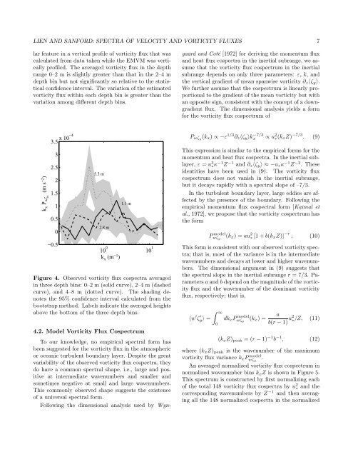
lar feature <strong>in</strong> a vertical pr<strong>of</strong>ile <strong>of</strong> <strong>vorticity</strong> flux that was<br />
calculated from data taken while the EMVM was vertically<br />
pr<strong>of</strong>iled. The averaged <strong>vorticity</strong> flux <strong>in</strong> the depth<br />
r<strong>an</strong>ge 0–2 m is slightly greater th<strong>an</strong> that <strong>in</strong> the 2–4 m<br />
depth b<strong>in</strong> but not signific<strong>an</strong>tly so relative to the statistical<br />
confidence <strong>in</strong>terval. The variation <strong>of</strong> the estimated<br />
<strong>vorticity</strong> flux with<strong>in</strong> each depth b<strong>in</strong> is greater th<strong>an</strong> the<br />
variation among different depth b<strong>in</strong>s.<br />
To our knowledge, no empirical spectral form has<br />
been suggested for the <strong>vorticity</strong> flux <strong>in</strong> the atmospheric<br />
or oce<strong>an</strong>ic turbulent boundary layer. Despite the great<br />
variability <strong>of</strong> the observed <strong>vorticity</strong> flux cospectra, they<br />
do have a common spectral shape, i.e., large <strong><strong>an</strong>d</strong> positive<br />
at <strong>in</strong>termediate wavenumbers <strong><strong>an</strong>d</strong> smaller <strong><strong>an</strong>d</strong><br />
sometimes negative at small <strong><strong>an</strong>d</strong> large wavenumbers.<br />
This commonly observed shape suggests the existence<br />
<strong>of</strong> a universal spectral form.<br />
Follow<strong>in</strong>g the dimensional <strong>an</strong>alysis used by Wyngaard<br />
<strong><strong>an</strong>d</strong> Coté [1972] for deriv<strong>in</strong>g the momentum flux<br />
<strong><strong>an</strong>d</strong> heat flux cospectra <strong>in</strong> the <strong>in</strong>ertial subr<strong>an</strong>ge, we assume<br />
that the <strong>vorticity</strong> flux cospectrum <strong>in</strong> the <strong>in</strong>ertial<br />
subr<strong>an</strong>ge depends on only three parameters: ε, k, <strong><strong>an</strong>d</strong><br />
the vertical gradient <strong>of</strong> me<strong>an</strong> sp<strong>an</strong>wise <strong>vorticity</strong> ∂ z 〈ζ y 〉.<br />
We further assume that the cospectrum is l<strong>in</strong>early proportional<br />
to the gradient <strong>of</strong> the me<strong>an</strong> <strong>vorticity</strong> but with<br />
<strong>an</strong> opposite sign, consistent with the concept <strong>of</strong> a downgradient<br />
flux. The dimensional <strong>an</strong>alysis yields a form<br />
for the <strong>vorticity</strong> flux cospectrum <strong>of</strong><br />
k x P wζy (m s −2 )<br />
3.5 x 10⁻⁴<br />
3<br />
2.5<br />
2<br />
1.5<br />
1<br />
0.5<br />
0<br />
−0.5<br />
5.3 m<br />
2.8 m<br />
1.1 m<br />
10 0 10 1<br />
k x (m −1 )<br />
Figure 4. Observed <strong>vorticity</strong> flux cospectra averaged<br />
<strong>in</strong> three depth b<strong>in</strong>s: 0–2 m (solid curve), 2–4 m (dashed<br />
curve), <strong><strong>an</strong>d</strong> 4–8 m (dotted curve). The shad<strong>in</strong>g denotes<br />
the 95% confidence <strong>in</strong>terval calculated from the<br />
bootstrap method. Labels <strong>in</strong>dicate the averaged heights<br />
above the bottom <strong>of</strong> the three depth b<strong>in</strong>s.<br />
4.2. Model Vorticity Flux Cospectrum<br />
P wζy (k x ) ∝ −ε 1/3 ∂ z 〈ζ y 〉k −7/3<br />
x ∝ u 2 ∗(k x Z) −7/3 . (9)<br />
This expression is similar to the empirical forms for the<br />
momentum <strong><strong>an</strong>d</strong> heat flux cospectra. In the <strong>in</strong>ertial sublayer,<br />
ε = u 3 ∗κ −1 Z −1 <strong><strong>an</strong>d</strong> ∂ z 〈ζ y 〉 ≈ −u ∗ κ −1 Z −2 . These<br />
identities have been used <strong>in</strong> (9). The <strong>vorticity</strong> flux<br />
cospectrum does not v<strong>an</strong>ish <strong>in</strong> the <strong>in</strong>ertial subr<strong>an</strong>ge,<br />
but it decays rapidly with a spectral slope <strong>of</strong> –7/3.<br />
In the turbulent boundary layer, large eddies are affected<br />
by the presence <strong>of</strong> the boundary. Follow<strong>in</strong>g the<br />
empirical momentum flux cospectral form [Kaimal et<br />
al., 1972], we propose that the <strong>vorticity</strong> cospectrum has<br />
the form<br />
P model<br />
wζ y<br />
(k x ) = au 2 ∗ [1 + b(k x Z)] −r . (10)<br />
This form is consistent with our observed <strong>vorticity</strong> spectra;<br />
that is, most <strong>of</strong> the vari<strong>an</strong>ce is <strong>in</strong> the <strong>in</strong>termediate<br />
wavenumbers <strong><strong>an</strong>d</strong> decays at lower <strong><strong>an</strong>d</strong> higher wavenumbers.<br />
The dimensional argument <strong>in</strong> (9) suggests that<br />
the spectral slope <strong>in</strong> the <strong>in</strong>ertial subr<strong>an</strong>ge r = 7/3. Parameters<br />
a <strong><strong>an</strong>d</strong> b depend on the magnitude <strong>of</strong> the <strong>vorticity</strong><br />
flux <strong><strong>an</strong>d</strong> the wavenumber <strong>of</strong> the dom<strong>in</strong><strong>an</strong>t <strong>vorticity</strong><br />
flux, respectively; that is,<br />
〈w ′ ζ ′ y〉 =<br />
∫ ∞<br />
0<br />
dk x Pwζ model a<br />
y<br />
(k x ) =<br />
b(r − 1) u2 ∗/Z, (11)<br />
(k x Z) peak = (r − 1) −1 b −1 , (12)<br />
where (k x Z) peak is the wavenumber <strong>of</strong> the maximum<br />
<strong>vorticity</strong> flux vari<strong>an</strong>ce k x P model<br />
wζ y<br />
.<br />
An averaged normalized <strong>vorticity</strong> flux cospectrum <strong>in</strong><br />
normalized wavenumber b<strong>in</strong>s k x Z is shown <strong>in</strong> Figure 5.<br />
This spectrum is constructed by first normaliz<strong>in</strong>g each<br />
<strong>of</strong> the total 148 <strong>vorticity</strong> flux cospectra by u 2 ∗ <strong><strong>an</strong>d</strong> the<br />
correspond<strong>in</strong>g wavenumbers by Z −1 <strong><strong>an</strong>d</strong> then averag<strong>in</strong>g<br />
all the 148 normalized cospectra <strong>in</strong> the normalized