Spectral characteristics of velocity and vorticity fluxes in an ...

More documents

Recommendations

Info

LIEN AND SANFORD: SPECTRA OF VELOCITY AND VORTICITY FLUXES 8 wavenumber bins. Note that ∼80% of spectra are observed in the bottom 4 m. The averaged, normalized vorticity flux cospectrum shows a wavenumber-bandlimited spectral shape similar to that of the momentum flux cospectrum. At small, normalized wavenumbers the lower bounds of the vorticity flux estimates are negative and show large error bars. The variancepreserving plot k x ZP wζy u −2 ∗ shows a peak at k x Z ≈ 2. The corresponding estimate of b is 3/8 based on (12). P wζy / u * 2 (a) 10 −2 10 −3 −7/3 10 −4 10 −1 10 0 10 1 k x Z 10 2 10 −1 k x Z P wζy /u * 2 0.4 0.35 0.3 0.25 0.2 0.15 0.1 0.05 (b) 10 −1 10 0 10 1 10 2 k x Z Figure 5. (a) Comparison of the observed vorticity flux cospectrum with our proposed model vorticity flux cospectrum. (b) The variance-preserving form of Figure 5a. The thick solid curve is the observed vorticity flux cospectrum calculated using spectra obtained in the bottom 8 m, and the thin curve is the model spectrum (equation (13)). The thick dashed curve is the observed vorticity flux cospectrum corrected for the sensor response function. A spectral slope of –7/3 is shown for comparison with the model spectrum in the inertial subrange. Open circles represent observed vorticity flux cospectra averaged using data in the bottom 5 m, where the observed vorticity flux follows the similarity scaling (Figure 7). In high-Reynolds-number flows one might expect the mixing coefficients of momentum and vorticity to have a similar magnitude. Indeed, Sanford and Lien [1999] found that the magnitudes of the estimated eddy diffusivity of vorticity [A ζ = −〈w ′ ζ y〉(∂ ′ z 〈ζ y 〉) −1 ] and the eddy viscosity of momentum [A ν = −〈u ′ w ′ 〉(∂ z U) −1 ] were similar within 6 mab. In the energetic tidal boundary layer the primary contribution to the mean spanwise vorticity is the vertical shear of streamwise velocity; that is, ζ y = ∂ z U [Sanford and Lien, 1999]. In the inertial sublayer the eddy viscosity of momentum A ν and the eddy diffusivity of vorticity A ζ can be approximated as u ∗ κZ, and the vertical gradient of the mean spanwise vorticity ∂ z 〈ζ y 〉 = −u ∗ κ −1 Z −2 . Therefore the turbulent vorticity flux in the inertial sublayer can be expressed as 〈w ′ ζ y〉 ′ = −A ζ ∂ z 〈ζ y 〉 = u 2 ∗Z −1 . Tennekes and Lumley [1972] similarly scaled the vorticity flux 〈w ′ ζ y〉 ′ as ul∂ z 〈ζ y 〉, where u = u ∗ is the turbulent velocity scale and l = κZ is the turbulent length scale in the boundary layer. Therefore the scaling of 〈w ′ ζ y〉 ′ = u 2 ∗Z −1 is also suggested by Tennekes and Lumley [1972]. If we accept the foregoing scaling argument for the turbulent vorticity flux, (11) can be expressed as a/[b(r− 1)] = 1. Given r = 7/3 and b = 3/8, the estimate of a is 1/2. Therefore we have constructed the following form for the model vorticity flux cospectrum: P model wζ y (k x ) = 1/2u 2 ∗ [1 + 3/8(k x Z)] −7/3 . (13) The model spectrum has the shape of observed spectra, the slope of –7/3 in the inertial subrange predicted by the dimensional analysis, and the dominant peak displayed by the observed spectra, and the magnitude of the vorticity flux is consistent with flows in the inertial sublayer. Note that when constructing the model spectrum, we have used only one property of the observed spectrum, the wavenumber of the maximum vorticity flux variance. We did not force the level and shape of the model spectrum to agree with those of the observed spectrum. Surprisingly, the model spectrum clearly reproduces the observed vorticity flux cospectrum (Figure 5) in the wavenumber range from the peak of the vorticity flux variance extending more than 1 decade into the inertial subrange where a spectral slope of –7/3 exists. At low wavenumbers, k x Z ≤ 0.9, the observed vorticity flux spectrum drops much more rapidly than the proposed model spectrum. Although the vorticity flux cospectrum and the momentum flux cospectrum have a very similar spectral shape, the wavenumber of the maximum flux is higher for the vorticity flux than for the momentum flux. This is partially because most of the turbulent momentum is at large scales and the variance of vorticity is mostly contributed by smaller-scale eddies. To correct for the finite-size-sensor effect, we modify the observed vorticity flux cospectra by their response functions (Appendix A) and form the composite spectrum. The corrected cospectrum is not significantly different from the uncorrected one, except at k x Z ≥ 40, where the corrected spectrum shows a small bump. We suspect that this small bump is unreal and is caused by dividing the observed spectrum by a response func-
LIEN AND SANFORD: SPECTRA OF VELOCITY AND VORTICITY FLUXES 9 tion that is small. On the basis of the EMVM response function for the vorticity flux cospectrum (Appendix A) and our model spectrum, the EMVM resolves > 90% of the total vorticity flux at Z > 1 m (Appendix B). 5. Discussion and Summary 5.1. Vorticity Flux Quad Spectrum of Isotropic Turbulence Note that the vorticity flux quad spectrum Q wζy of the isotropic turbulence does not vanish [Batchelor, 1959]. We calculate the composite quad spectrum of the measured vorticity flux, correct for the sensor response function, and compare the result with the expected quad spectrum in the inertial subrange, as predicted by (4) (Figure 6). The response function of the quad spectrum is based on the theoretical quad-spectral form of Batchelor [1959] for isotropic turbulence. 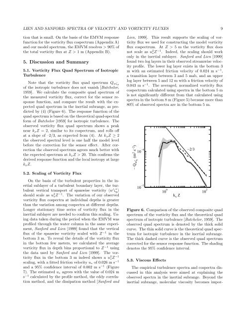The observed vorticity flux quad spectrum shows a peak near k x Z = 2, similar to its cospectrum, and rolls off at a slope of –2/3, as expected from (4). At k x Z ≥ 2 the observed spectral level is one half the model level before the correction for the sensor effect. After correction the observed spectrum agrees much better with the expected spectrum at k x Z > 20. This confirms the derived response function and the local isotropy at large k x Z. 5.2. Scaling of Vorticity Flux On the basis of the turbulent properties in the inertial sublayer of a turbulent boundary layer, the turbulent vertical transport of spanwise vorticity 〈w ′ ζ y〉 ′ should scale as u 2 ∗Z −1 . The variation of our observed vorticity flux cospectra at individual depths is greater than the variation among cospectra at different depths. Longer stationary time series of vorticity flux in the inertial sublayer are needed to confirm this scaling. Using data taken during the period when the EMVM was profiled through the water column in the same experiment, Sanford and Lien [1999] found that the vertical flux of the spanwise vorticity scaled with Z −1 in the bottom 3 m. To reveal the details of the vorticity flux in the bottom few meters, we calculated the average vorticity flux in depth bins proportional to Z −1 using the data used by Sanford and Lien [1999]. The vorticity flux in the bottom 3 m indeed shows a u 2 ∗Z −1 scaling, with a fitted friction velocity u ∗ of 0.026 m s −1 and a 95% confidence interval of 0.002 m s −1 (Figure 7). The estimated u ∗ agrees with the value of 0.024 m s −1 calculated by the profile method, the eddy correlation method, and the dissipation method [Sanford and Lien, 1999]. This result supports the scaling of vorticity flux we used for constructing the model vorticity flux cospectrum. At Z > 5 m the vorticity flux does not scale as u 2 ∗Z −1 . Indeed, the scaling should work only in the inertial sublayer. Sanford and Lien [1999] found two log layers in their observed streamwise velocity profile. The lower log layer exists in the bottom 3 m with an estimated friction velocity of 0.024 m s −1 , a transition layer between 3 and 5 mab, and an upper log layer between 5 and 12 m with a friction velocity of 0.043 m s −1 . The averaged, normalized vorticity flux cospectrum calculated using spectra in the bottom 5 m is not significantly different from that calculated using spectra in the bottom 8 m (Figure 5) because more than 80% of observed spectra are in the bottom 5 m. − Q wζy (m 2 s −2 ) −2/3 10 −4 10 −5 10 0 10 2 k x Z Figure 6. Comparison of the observed composite quad spectrum of the vorticity flux and the theoretical quad spectrum of isotropic turbulence [Batchelor, 1959]. The observed quad spectrum is denoted by the thick solid curve. The thin solid curve is the theoretical quad spectrum for isotropic turbulence in the inertial subrange. The thick dashed curve is the observed quad spectrum corrected for the sensor response function. The shading denotes the 95% confidence interval. 5.3. Viscous Effects The empirical turbulence spectra and cospectra discussed in this analysis were aimed at explaining the observed spectra in the inertial subrange. Beyond the inertial subrange, molecular viscosity becomes impor-
Page 1 and 2: Spectral characteristics of velocit
Page 3 and 4: LIEN AND SANFORD: SPECTRA OF VELOCI
Page 7: LIEN AND SANFORD: SPECTRA OF VELOCI
Page 13: LIEN AND SANFORD: SPECTRA OF VELOCI

Spectral characteristics of velocity and vorticity fluxes in an ...

Create successful ePaper yourself

Delete template?

Save as template?