Approaching predator-prey Lotka-Volterra Equations by Simplicial ...

Proceedings of the 4th International Workshop
on Compositional Data Analysis (2011)
Approaching predator-prey Lotka-Volterra equations by
simplicial linear differential equations
E. JARAUTA-BRAGULAT 1 and J. J. EGOZCUE 1
1 Dept. Matemàtica Aplicada III, U. Politècnica de Catalunya, Barcelona, Spain (eusebi.jarauta@upc.edu)
Abstract
Predator-prey Lotka-Volterra equations was one of the first models reflecting interaction of different species and
modeling evolution of respective populations. It considers a large population of hares (preys) which is depredated
by an also large population of lynxes (predators). It proposes an increasing/decreasing law of the number of
individuals in each population thus resulting in an apparently simple system of ordinary differential equations.
However, the Lotka-Volterra equation, and most of its modifications, is non-linear and its generalization to a
larger number of species is not trivial. The present aim is to study approximations of the evolution of the
proportion of species in the Lotka-Volterra equations using some simple model defined in the simplex.
Calculus in the simplex has been recently developed on the basis of the Aitchison geometry and the simplicial
derivative. Evolution of proportions in time (or other parameters) can be represented as simplicial ordinary
differential equations from which the simpler models are the linear ones. Simplicial Linear Ordinary Differential
Equations are not able to model the evolution of the total mass of the population (total number of predators plus
preys) but only the evolution of the proportions of the different species (ratio predators over preys). This way of
analysis has been successful showing that the compositional growth of a population in the Malthusian exponential
model and the Verhulst logistic model were exactly the same one: the first order simplicial linear differential
equation with constant coefficients whose solution is a compositional straight-line. This strategy of studying the
total mass evolution and the compositional evolution separately is used to get a simplicial differential equation
whose solutions approach suitably the compositional behavior of the Lotka-Volterra equations. This approach
has additional virtues: it is linear and can be extended in an easy way to a number of species larger than two.
1 Introduction
Systems of ordinary differential equations have been frequently used to model the behaviour of populations,
understanding populations in a wide sense: biological, human, resources, epidemia, etc. (Bacaër,
2011). The population is partitioned into classes of individuals and the number of individuals in each
class is treated as a continuous real variable. This continuous number of individuals of a class will be
called mass of the class. Elementary models express the derivative of the mass of a class as a simple
function of the number of all masses. Solutions of this kind of differential equations are generically
known as growth curves (Odum, 1971). The simplest and older model is the exponential growth model
which appear in bacteria growth, human communities (Euler, 1760), radioactive decay, etc. and it can
be formulated as
Dm i (t) = k i m i (t) , i = 1, 2, . . . , n , (1)
where m i (t) represents the mass of the i-th class as a function of time t; D is the ordinary derivative
operator with respect to t and n is the number of classes. Model (1) can be complemented with new
classes of individuals without changing the meaning of the equations. For instance, the traditional
Euler-Malthus model is Dm 1 = k 1 m 1 being m 1 the individuals of a human population and k 1 > 0. If
m 1 (0) is the initial mass, the solution of the differential equation is m 1 (t) = m 1 (0) exp(k 1 t), t ≥ 0. We
can redefine the population as made of resources cells: some of them, m 1 (t), occupied by individuals;
and those cells which are available, m 2 (t). Assuming that m 2 (t) is a constant it satisfies the differential
equation Dm 2 = 0. Solving for the system (1), with n = 2, k 1 > 0, k 2 = 0, the solution of the mass
m 1 (t) is exactly the previous one.
An apparently more complex model is the logistic one (Verhulst, 1838). It can be written as
Dm 1 (t) = k 1 m 1 (t) (m ∞ 1 − m 1 (t)) , k 1 > 0 , (2)
Egozcue, J.J., Tolosana-Delgado, R. and Ortego, M.I. (eds.)
ISBN: 978-84-87867-76-7
1
1

Proceedings of the 4th International Workshop
on Compositional Data Analysis (2011)
which is a non linear-Ricatti equation whose solution is the well known logistic curve, and m ∞ 1 is the
asymptotic mass of population. Again equation (2) can be complemented with an equation for the
available resource cells. An option is m 2 = M −m 1 , M > 0, or equivalently Dm 2 = −k 1 m 1 (m ∞ 1 −m 1)
which maintains the solution for m 1 (t) unaltered.
Another class of models of population growth is the so called SIR-models (and generalisations).
Let m 1 ≡ S, m 2 ≡ I, m 3 ≡ R the mass of susceptible to a disease, the mass of infected people, and the
mass of recovered people, respectively. Whenever the latent evolution of the population is neglected
the SIR-model (Kermack and McKendrick, 1927) is
Dm 1 (t) = −αm 1 (t)m 2 (t) , Dm 2 (t) = αm 1 (t)m 2 (t) − γm 2 (t) , Dm 3 (t) = γm 2 (t) , (3)
for some positive constants α, γ. This model has been successfully used in prediction of epidemics
evolution.
Also predator-prey Lotka-Volterra equations, and their sequels, corresponds to the same type of
equations. If m 1 represents the mass of predators, m 2 the mass of preys then Lotka-Volterra equations
are
Dm 1 (t) = −a 1 m 1 (t) + a 2 m 1 (t)m 2 (t) , Dm 2 (t) = b 1 m 2 (t) − b 2 m 1 (t)m 2 (t) , (4)
where the coefficients a 1 , a 2 , b 1 , b 2 are assumed positive. Despite of the apparent simplicity of these
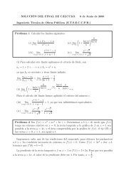
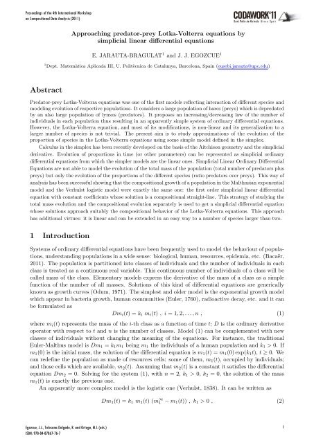
equations, their solution is not explicit although the orbit (m 1 (t), m 2 (t)) is easily obtained. Figure 1
(left) shows predator-prey (lynx-hare) data used in Section 4 as an example and at the right panel one
cycle orbit described by observed data (blue) and the orbit of the solution of Lotka-Volterra equations
fitted to the data set.
All cited examples can be viewed in two different ways: the traditional representation using masses
of each class as in equations (1), (2), (3), (4); an alternative consisting of representing the system as an
equation for the total mass m(t) = ∑ i m i(t) and a simplicial differential equation for the composition
containing the proportion of masses, i.e. x(t) = C(m 1 (t), m 2 (t), . . . , m n (t)) ∈ S n where C is the closure
to unit and S n the n-part simplex. The difference between these two representations is the metric
of the space where the solutions are defined. In the traditional case, masses evolve in R n + assuming
that the metric is inherited from the Euclidean space R n . In the second case, the representation, total
mass and composition, is a curve in the space R + × S n which is also a n-dimensional Euclidean space
(Pawlowsky-Glahn and Egozcue, 2001). This strategy separating the compositional model from the
total mass evolution has been successful proving that the compositional differential equation for the
Euler-Malthus Eq. (1), with n = 2, k 1 > 0, k 2 = 0, and the logistic Verhulst model (2) are just
equal, and they only differ in the behaviour of the total mass (Jarauta-Bragulat and Egozcue, 2008,
2010). Moreover, in the case of the logistic model (2), the compositional equation is a first order
linear equation which is simpler than the Eq. (2) itself. This previous results suggest that, in some
cases, models expressed in mass may be simplified or approached studying their compositional and
total mass models separately.
Attention is now focussed in the Lotka-Volterra system (4). The main idea is that these equations
can be approached by simple compositional and total mass models. These simple models have been
chosen to be harmonic oscillators (Section 4) for the total mass and for the compositional part being
the natural frequency equal in both equations.
2 Linear differential equations in S n and R +
Derivatives on the simplex
Simplicial derivatives have been defined in Aitchison (1986) (postscript 2003 printing) and also in
Aitchison et al. (2002), Egozcue et al. (2008). A more detailed development is found in Egozcue et al.
(2011). If f : R → S n is a function of a real variable (time) on the simplex (proportions of masses),
the simplicial derivative of f at t is defined as
( )
1
D ⊕ f(t) = lim
h→0 h ⊙ (f(t + h) ⊖ f(t)) , (5)
Egozcue, J.J., Tolosana-Delgado, R. and Ortego, M.I. (eds.)
ISBN: 978-84-87867-76-7
2

Proceedings of the 4th International Workshop
on Compositional Data Analysis (2011)
250
100
200
75
Indivuduals (thousands)
150
100
thousands of hares
50
50
25
0
0 10 20 30 40 50
time (year)
lynxes hares mass
0
0 25 50 75 100
thousands of lynxes
Figure 1: Left, observed number (in thousands) of hares and lynxes 1885-1935 (Odum, 1971). Right, periodic orbits of
(m 2, m 1) as observed (blue), for fitted Lotka-Volterra equations (LV, red) and the proposed harmonic oscillator
(HO, green) fitted to data. The central dot is the equilibrium value estimated for both LV and HO.
if the limit exists. In Equation (5), standard notation of operations in the simplex is adopted: ⊕ is
perturbation and ⊖ is the opposite of perturbation; ⊙ denotes powering by real scalars. Computation
of the derivative is easily carried out using logarithmic derivatives,
(
D ⊕ Df1 (t)
f(t) = C exp (D log(f(t))) = C exp
f 1 (t) , . . . , Df )
n(t)
, (6)
f n (t)
where functions (exp, log, . . . ) operate componentwise on vectors. Moreover, f is not necessarily closed
to unit because any equivalent (proportional) function gives the same result. A further simplification
consists of expressing the compositional function in coordinates with respect to any orthonormal basis.
If ilr : S n → R n−1 assigns orthonormal coordinates to any composition (Egozcue et al., 2003; Egozcue
and Pawlowsky-Glahn, 2005, 2006), then
D ⊕ f(t) = ilr −1 (D(ilr(f))) , (7)
where again D denotes derivative with respect to the real variable (time).
Using expressions Eq. (6) and (7), K-order simplicial linear (ordinary) differential equations
(SLODE) expressed in the simplex are
K⊕
a k ⊙ (D ⊕ ) k x(t) = ϕ(t) ,
k=0
being (D ⊕ ) k the k-th simplicial derivative ((D ⊕ ) 0 is the identity) and ϕ a forcing compositional term.
Once an orthonormal basis of the simplex is selected, the compositional functions x(t) and ϕ(t) can
be expressed using their coordinates, i.e. x ∗ (t) = (x ∗ 1 (t), x∗ 2 (t), . . . , x∗ n−1 (t)) = ilr(x(t)) (analogously
for ϕ(t)), given rise to a system of n − 1 linear ordinary differential equations
K∑
a k · D k x ∗ (t) = ϕ ∗ (t) .
k=0
Methods for solving this kind of differential equations are well-known and can be applied without any
restriction. Once a solution for the coordinates x ∗ is known it can be immediately translated into the
compositional solution as x = ilr −1 (x ∗ ).
Derivatives in R +
Whenever a relative scale in R + is assumed, differences are no longer measured by ordinary differences
but logarithmic differences (Pawlowsky-Glahn and Egozcue, 2001). Therefore, a derivative of a
Egozcue, J.J., Tolosana-Delgado, R. and Ortego, M.I. (eds.)
ISBN: 978-84-87867-76-7
3

Proceedings of the 4th International Workshop
on Compositional Data Analysis (2011)
function f : R → R + needs a re-definition. The idea is that R + is a one-dimensional Euclidean space,
where the group operation (addition, also denoted ⊕) is the ordinary product and the external operation
(denoted ⊙) is powering. Similarly to the simplex, a basis can be defined so that any element
in R + can be represented by its coordinate with respect to the basis. A simple choice of a basis in
R + is the number e = exp(1) which allows the coordinate expression x = exp(log x) for any x ∈ R + .
Therefore, log x ∈ R is the coordinate of x ∈ R + when the selected basis is e. After these concepts,
the derivative for the coordinates of functions in R + is
D(log f(t)) = lim
h→0
log f(t + h) − log f(t)
h
which translated back to R + gives the desired derivative
D + f(t) = exp (D(log f(t))) ,
,
which clearly recalls derivatives in the simplex (5-7).
Differential equations in R + can be equivalently written using D + or using coordinates.
instance, a K-order linear differential equation in R + is
For
K⊕
a k ⊙ (D + ) k x(t) = ϕ(t) ,
k=0
where, for x, y ∈ R + , α ∈ R, x ⊕ y = exp(log x + log y) = xy, α ⊙ x = exp(α log x) = x α ; x(t) is the
unknown positive function and ϕ(t) represents a positive forcing term. This equation can be written
in coordinates
K∑
a k · D k x ∗ (t) = f ∗ (t) , x ∗ (t) = log x(t) , ϕ ∗ (t) = log ϕ(t) ,
k=0
which is a linear ordinary differential equation in R.
Total mass and compositional models
An important point is how to get the total mass and the compositional evolution equations from the
differential equations for masses of the classes. There are essentially two ways to do it. The first one
is to solve the system in masses; then, compute proportions and their representation in coordinates;
and finally, obtain the simplicial differential equations from the solution in coordinates. Although
apparently simple, this way is plenty of difficulties: the solution in mass should be explicit and also
the solution in coordinates; and afterwards, the identification of the differential equation should be
feasible. A second way, which may be considered standard, starts transforming the derivatives of the
differential equation in mass into logarithmic derivatives, and then, expressing the remaining term
in a compositional way. Even simple equations in mass can exhibit unexpected links between the
compositional part of the equation and the total mass equation. If this is the case, little benefit
is obtained from expressing the equations of the system as compositional and total mass equations.
However, if the compositional and total mass equations are not coupled, then the interpretation of the
model is simplified.
3 Lotka-Volterra equations
The predator-prey Lotka-Volterra equations (4) are
Dm 1 (t) = −a 1 m 1 (t) + a 2 m 1 (t)m 2 (t) , Dm 2 (t) = b 1 m 2 (t) − b 2 m 1 (t)m 2 (t) , (8)
where m 1 (t) is the mass of predators, m 2 (t) is the mass of preys and m(t) = m 1 (t) + m 2 (t) is the
total mass. It is interesting to pay attention to the reasoning that leads to both equations in (8). It
can be summarised as: the mass of predators decreases proportionally to the predator mass because
predator individuals compite for their territory; and the mass of predators increases proportionally to
Egozcue, J.J., Tolosana-Delgado, R. and Ortego, M.I. (eds.)
ISBN: 978-84-87867-76-7
4

Proceedings of the 4th International Workshop
on Compositional Data Analysis (2011)
the number of encounters between predators and preys which is the way of feeding predators; moreover,
the number of predator-prey encounters is proportional to the product of masses of predators and preys.
Similarly, the mass of preys increases proportionally to preys mass, provided there is enough vegetal
food for preys; and decreases proportionally to the number of predator-prey encounters because some of
them conclude with the dead of the prey. This kind of reasoning has three remarkable characteristics:
(a) there is no mention of the total mass of predators and preys and it is not sensible to the mass
of individuals; (b) it implicitly assumes that the way of measuring change of mass is the ordinary
derivative for real functions with the ordinary way of measuring differences; (c) when it is said that
the increase/decrease of the mass is proportional to two quantities, the two proportionality effects on
the change are assumed additive.
Characteristic (a) points out the compositional character that should be present in the equation.
However, Eq. (8) is not scale invariant and the influence of encounters depends on the masses and
not only on their proportions. Point (b) assumes, e.g., that the difference in mass of 100 and 1, 000
individuals is exactly the same as between 1 million and 1 million plus 900 individuals, against the
appreciation of an ecologist that probably feels that 100 is a critical number of individuals for a population
near of extinction; 1000 individuals is dangerous but not critical; and 1, 000, 000 and 1, 000, 900
individuals in two populations are very similar masses. Probably, the ecologist would better understand
that for measure these differences is better to compare the numbers using ratios, 1, 000/100 = 10,
(10 6 + 900)/10 6 ≈ 1. A little step further is to measure the ratio differences taking their logarithm
so that symmetrizing the role of numerator and denominator: in the first case log(10 3 /10 2 ) ≃ 2.3
and the second one log((10 6 + 9 · 10 2 )/10 6 ) ≃ 8 · 10 −4 . Characteristic (c) is a little bit mysterious.
Reasoning mainly mentions proportionality and additivity does not take place. One can think this
was introduced to get a simple equation, but many aspects of Lotka-Volterra equations (8) are not
simple, and finally the equations must be solved numerically.
Proportion of predators and preys over the total is denoted x = (x 1 , x 2 ) = C(m 1 , m 2 ). Transforming
Eq. (8) to express it using logarithmic derivatives, this is
D log m 1 (t) = −a 1 + a 2 m 2 (t) , D log m 2 (t) = b 1 (t) − b 2 m 1 (t) .
Since x is a composition of two parts, it is represented by a single coordinate x ∗ = 2 −1/2 log(x 1 /x 2 ).
The derivative Dx ∗ is the coordinate expression of the simplicial derivative
D ⊕ x = C exp(D log(m 1 , m 2 )) = C exp(D log(x 1 , x 2 )) .
After some algebra
Dx ∗ = √ 1
)
(−(a 1 + b 1 ) + e m∗ (a 2 x 2 + b 2 x 1 )
2
, Dm ∗ = −(a 1 x 1 − b 1 x 2 ) + e m∗ (a 2 − b 2 )x 1 x 2 , (9)
where the proportions x = (x 1 , x 2 ) can be expressed as a function of the coordinate (balance) x ∗ and
the coordinate of m in R + , m ∗ = log m (Pawlowsky-Glahn and Egozcue, 2001). The expressions for
x 1 and x 2 are
x 1 = exp(√ 2 x ∗ )
1 + exp( √ 2 x ∗ )
, x 2 =
1
1 + exp( √ 2 x ∗ ) ,
which
√
is the ilr −1 transformation into S 2 , and also the inverse logit transform up to the constant
2. Although Equations (9) are numerically tractable, they are coupled and they do not offer any
advantage over the original Lotka-Volterra equations (8).
After these equations using coordinates in R + × S 2 and the criticisms to the underlaying ideas to
Lotka-Volterra equations, to approach these equations with a simple total mass-compositional model
seems advisable.
4 A simple model approaching Lotka-Volterra equations
Lotka-Volterra equations have periodic solutions (Fig. 1, right). This means that the approaching
equations should have solutions for coordinate in S 2 and coordinate in R + which must be also periodic.
Egozcue, J.J., Tolosana-Delgado, R. and Ortego, M.I. (eds.)
ISBN: 978-84-87867-76-7
5

Proceedings of the 4th International Workshop
on Compositional Data Analysis (2011)
160
thousands of hares
140
120
100
80
60
40
20
0
0 5 10 15 20 25 30 35 40 45 50
time (year)
data LV HO
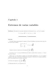
Figure 2: Mass, in thousands, of hares (left) and lynxes (right). Observed 1885-1935 (Odum, 1971) (blue); for fitted
Lotka-Volterra equations (red) and the proposed harmonic oscillator (green).
160
140
140
120
Indivuduals (thousands)
120
100
80
60
40
20
Indivuduals (thousands)
100
80
60
40
20
0
0 10 20 30 40 50
time (year)
lynxes hares mass
0
0 10 20 30 40 50
time (year)
lynxes hares mass
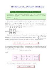
Figure 3: Comparison in time (1885-1935) of number (in thousands) of lynxes, hares and total individuals for the fitted
Lotka-Volterra equations (LV, left) and for the fitted harmonic oscillator (HO, right).
For simplicity, linear differential equations are preferred as approaching equations, but periodic solutions
are only attained with linear differential equations of order 2 or higher. The simplest model in
R + × S 2 , stated in coordinates, and with periodic solutions is the free oscillating, uncoupled harmonic
oscillator
D 2 µ ∗ + ω 2 µ ∗ = 0 , D 2 y ∗ + ω 2 y ∗ = 0 , (10)
with a single parameter ω which represents the natural angular frequency of oscillation around the
point µ ∗ = 0, y ∗ = 0. Since orbits of Lotka-Volterra equations are centered on a point which is
determined by the coefficients a 1 , a 2 , b 1 , b 2 (8), a shift of the oscillator (10) adapts the oscillator to the
Lotka-Volterra system. This can be done defining m ∗ = m ∗ 0 +µ∗ and x ∗ = x ∗ 0 +y∗ , where m ∗ 0 = log m 0,
x ∗ 0 = 2−1/2 log(x 10 /x 20 ) represents a shift in coordinates of R + × S 2 ; m 0 is a multiplicative change
in total mass and (x 10 , x 20 ) is a perturbation (shift) in S 2 . This completes a three parameter model
which are ω, m ∗ 0 , and x∗ 0
The general solution of the oscillator (10) is explicit
m ∗ (t) = m ∗ 0 + A m sin(ωt) + B m cos(ωt) , x ∗ (t) = x ∗ 0 + A x sin(ωt) + B x cos(ωt) , (11)
where the constants m ∗ 0 , x∗ 0 , correspond to mean values and A m, B m , A x , B x are determined by initial
or boundary conditions.
To show the effectiveness of the proposed approach, a demonstration data set for the Lotka-
Volterra equation have been used (Odum, 1971). It corresponds to 1845-1935 year record of the mass
of lynxes (predators m 1 ) and mass of hares (preys m 2 ). Only data for years 1885-1935 are used in the
present example as measurements are more reliable. Masses are measured in thousands of individuals.
Parameters of Lotka-Volterra (LV) and the harmonic oscillator (HO) in Equation 11 have been fitted
Egozcue, J.J., Tolosana-Delgado, R. and Ortego, M.I. (eds.)
ISBN: 978-84-87867-76-7
6

Proceedings of the 4th International Workshop
on Compositional Data Analysis (2011)
Table 1: Parameters for Lotka-Volterra (LV) equations and the harmonic oscilator (HO) fitted to data. T is the estimated
period in year corresponding to ω.
Lotka-Volterra
a 1 = 0.842 a 2 = 0.019
b 1 = 0.473 b 2 = 0.016
harmonic oscillator
eq. coordinates eq. R + × S n
m ∗ 0 = 4.276 m 0 = 71.953 thousands
x ∗ 0 = −0.273 x 10 = 0.405
x 20 = 0.595
ω = 0.631 (years) −1
T = 9.957 years
3.0
6.0
2.0
5.0
1.0
4.0
0.0
3.0
-1.0
2.0
-2.0
1.0
-3.0
0 10 20 30 40 50
time (year)
ilr LV ilr HO ilr data
0.0
0 10 20 30 40 50
time (year)
log-mass LV log-mass HO log-mass data
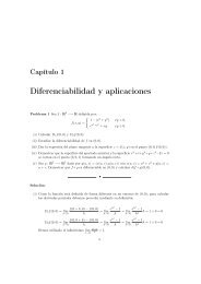
Figure 4: Comparison of the coordinates (ilr) of composition (lynxes,hares) and the log-total mass of lynxes (red), hares
(green) and total mass (blue) along 1885-1935. Left: ilr-coordinate x ∗ ; right: log-total mass (thousands) m ∗ .
using least squares. The procedure consists of the following steps: (a) express the data in coordinates
m ∗ (t i ) and x ∗ (t i ) for the sampling times t i ; (b) determine the equilibrium values m ∗ 0 , x∗ 0 as the mean
values along the coordinates; (c) determine the angular frequency ω using Pisarenko harmonic analysis
(Pisarenko, 1973) on the coordinates computed in (a); (d) using the estimated values of m ∗ 0 , x∗ 0 , ω,
determine a 1 , a 2 , b 1 , b 2 and solve numerically the Lotka-Volterra equations (8) using observed initial
conditions; (e) using the estimated values of m ∗ 0 , x∗ 0 , ω, determine the values A m, B m , A x , B x in
Equation (11) using least squares. The resulting parameters are shown in Table 1.
Figure 1 (left) shows the evolution of the mass of hares (blue) and lynxes (red) as observed along 50
years (1885-1935); also the total mass is reported. In Figure 1 (right) the orbit described by data in one
cycle is represented in blue. Also in Figure 1 (right), orbits for the fitted Lotka-Volterra (LV, red) and
harmonic oscilator (HO, green) are represented. They go around the equilibrium point m 01 = m 0 x 01
(lynxes), m 02 = m 0 x 02 (hares). The represented orbits appear quite different. However, one should
take into account the inconvenient scale of this representation where relative scale is ignored. The size
of the cycle of observed data corresponds to the first cycle which has an amplitude larger than the
rest of the signal; other cycles would appear smaller than the represented one. Further comparisons of
data, LV and HO are shown in time in Figure 2. An overestimation of the amplitude in LV is apparent.
Also LV appears to be slightly shifted in its maxima-minima with respect to data. This is mainly
due to the procedure of solving Lotka-Volterra equations (8) which is based on initial conditions and,
consequently, the obtained solution will be sensible to the initial point and not to the rest of the
time-series. Here, an inconvenient of non-simple model clearly appear: solution cannot be easily fitted
to data and initial conditions are used instead. This is not the case of HO because the solution is
explicit (11).
Figure 3 shows the joint behaviour of mass of lynxes (red), of hares (green) and total mass (blue) for
Egozcue, J.J., Tolosana-Delgado, R. and Ortego, M.I. (eds.)
ISBN: 978-84-87867-76-7
7

Proceedings of the 4th International Workshop
on Compositional Data Analysis (2011)
LV (right) and HO (left). Qualitative comparison of left and right figures reveals a similar behaviour
of the two models thus justifying the approach using the harmonic oscillator. Figure 4 shows the
behaviour of coordinates of total mass, m ∗ (t) (right), and the composition (lynxes, hares), x ∗ (t) (left),
for the data, LV and HO. Again the qualitative behaviour of LV (red) and HO (sinusoidal) (green)
appears to be quite similar. Particularly, log-total mass is almost sinusoidal for LV. Figure 4 also
shows that the model fits the data poorly for both LV and HO. It appears that there are changes in
the oscillating period and in amplitude. This may suggest that introducing forcing terms in Equations
(10) may be convenient to model interactions of the system with the environment.
5 Conclusions
Many models of population evolution have been formulated as systems of ordinary differential equations
for the number of individuals of each considered class. An alternative formulation is proposed:
modelling the evolution of the total of individuals as a function of time in R + , and the evolution of
the proportions of individuals as a function of time in the simplex. Both functions can be represented
in coordinates of the respective spaces using ordinary differential equations for these coordinates.
The predator-prey Lotka-Volterra equations have been examined. Despite of reasoning leading to
the equations are mainly compositional, the equations themselves are not scale invariant thus putting
forward some criticism on the model. Following the idea of modelling total mass and composition
in coordinates of R + × S n and using differential equations, a simple uncoupled harmonic oscillator
is proposed to approach the dynamics of a predator-prey population which solutions satisfactorily
approach those of the corresponding Lotka-Volterra equations.
References
Aitchison, J. (1986). The Statistical Analysis of Compositional Data. Monographs on Statistics and
Applied Probability. Chapman & Hall Ltd., London (UK). (Reprinted in 2003 with additional
material by The Blackburn Press). 416 p.
Aitchison, J., C. Barceló-Vidal, J. J. Egozcue, and V. Pawlowsky-Glahn (2002). A concise guide for the
algebraic-geometric structure of the simplex, the sample space for compositional data analysis. In
U. Bayer, H. Burger, and W. Skala (Eds.), Proceedings of IAMG’02 — The eigth annual conference of
the International Association for Mathematical Geology, Volume I and II, pp. 387–392. Selbstverlag
der Alfred-Wegener-Stiftung, Berlin, 1106 p.
Bacaër, N. (2011). A Short History of Mathematical Population Dynamics. Springer, Berlin. 160p.
Egozcue, J. J., E. Jarauta-Bragulat, and J.-L. Díaz-Barrero (2011). Calculus of simplex-valued functions.
In V. Pawlowsky-Glahn and A. Buccianti (Eds.), Wiley, in press.
Egozcue, J. J. and V. Pawlowsky-Glahn (2005). Groups of parts and their balances in compositional
data analysis. Mathematical Geology 37 (7), 795–828.
Egozcue, J. and V. Pawlowsky-Glahn (2006). Simplicial geometry for compositional data. In Compositional
Data Analysis in the Geosciences: From Theory to Practice, Buccianti, A. and Mateu-
Figueras, G. and Pawlowsky-Glahn, V. (eds), Vol. 264 of Special Publications. Geological Society,
London.
Egozcue, J. J., V. Pawlowsky-Glahn, and J. L. Díaz-Barrero (2008). Otros espacios euclídeos. La
Gaceta de la Real Sociedad Matemática Española 11 (2), 263–267.
Egozcue, J. J., V. Pawlowsky-Glahn, G. Mateu-Figueras, and C. Barceló-Vidal (2003). Isometric
logratio transformations for compositional data analysis. Mathematical Geology 35 (3), 279–300.
Euler, L. (1760). Réchérches générales sur la mortalité et la multiplication du gendre humain. Hist.
Acad. R. Sci. B.-Lett. Berl. 16, 144–164.
Egozcue, J.J., Tolosana-Delgado, R. and Ortego, M.I. (eds.)
ISBN: 978-84-87867-76-7
8

Proceedings of the 4th International Workshop
on Compositional Data Analysis (2011)
Jarauta-Bragulat, E. and J. J. Egozcue (2008). Compositional evolution with mass transfer in closed
systems. In Proceedings of CODAWORK’08, The 3rd Compositional Data Analysis Workshop,
Daunis-i-Estadella, J. and Martín-Fernández, J.A. (Eds.), University of Girona, Girona (Spain).
Jarauta-Bragulat, E. and J. J. Egozcue (2010). An approach to growth curves analysis from a simplicial
point of view. In Proceedings of IAMG’10 — The XIVth annual conference of the International
Association for Mathematical Geosciences, Budapest (Hungary).
Kermack, W. O. and A. G. McKendrick (1927). A contribution to the mathematical theory of epidemics.
Proc. R. Soc. London 115, 700–721.
Odum, E. P. (1971). Fundamentals of Ecology. Saunders, W. Washington Square, Philadelphia.
Pawlowsky-Glahn, V. and J. J. Egozcue (2001). Geometric approach to statistical analysis on the
simplex. Stochastic Environmental Research and Risk Assessment (SERRA) 15 (5), 384–398.
Pisarenko, V. F. (1973). The retrieval of harmonics from a covariance function geophysics. J. Roy.
Astron. Soc. 33, 347–366.
Verhulst, P. F. (1838). Notice sur la loi que la population poursuit dans son accroyssement. Correspondance
Mathématique et Fysique 10, 113–121.
Egozcue, J.J., Tolosana-Delgado, R. and Ortego, M.I. (eds.)
ISBN: 978-84-87867-76-7
9