Math 211 Business Calculus Applications of Derivatives
Math 211 Business Calculus Applications of Derivatives
Math 211 Business Calculus Applications of Derivatives

Create successful ePaper yourself
Turn your PDF publications into a flip-book with our unique Google optimized e-Paper software.
– p. 1/34<br />
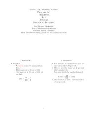
<strong>Math</strong> <strong>211</strong> <strong>Business</strong> <strong>Calculus</strong><br />
<strong>Applications</strong> <strong>of</strong> <strong>Derivatives</strong><br />
Pr<strong>of</strong>essor Richard Blecksmith<br />
richard@math.niu.edu<br />
Dept. <strong>of</strong> <strong>Math</strong>ematical Sciences<br />
Northern Illinois University<br />
http://math.niu.edu/∼richard/<strong>Math</strong><strong>211</strong>
– p. 2/34<br />
Asymptotes<br />
A nonvertical line with equation y = mx+b is called<br />
an asymptote <strong>of</strong> the graph <strong>of</strong> y = f(x)
– p. 2/34<br />
Asymptotes<br />
A nonvertical line with equation y = mx+b is called<br />
an asymptote <strong>of</strong> the graph <strong>of</strong> y = f(x) if the<br />
differencef(x)−(mx+b) tends to 0
– p. 2/34<br />
Asymptotes<br />
A nonvertical line with equation y = mx+b is called<br />
an asymptote <strong>of</strong> the graph <strong>of</strong> y = f(x) if the<br />
differencef(x)−(mx+b) tends to 0 asxtakes on<br />
arbitrarily large positive values
– p. 2/34<br />
Asymptotes<br />
A nonvertical line with equation y = mx+b is called<br />
an asymptote <strong>of</strong> the graph <strong>of</strong> y = f(x) if the<br />
differencef(x)−(mx+b) tends to 0 asxtakes on<br />
arbitrarily large positive values or arbitrarily large<br />
negative values.
– p. 2/34<br />
Asymptotes<br />
A nonvertical line with equation y = mx+b is called<br />
an asymptote <strong>of</strong> the graph <strong>of</strong> y = f(x) if the<br />
differencef(x)−(mx+b) tends to 0 asxtakes on<br />
arbitrarily large positive values or arbitrarily large<br />
negative values.<br />
Ifm = 0 theny = b is called a horizontal asymptote.
– p. 2/34<br />
Asymptotes<br />
A nonvertical line with equation y = mx+b is called<br />
an asymptote <strong>of</strong> the graph <strong>of</strong> y = f(x) if the<br />
differencef(x)−(mx+b) tends to 0 asxtakes on<br />
arbitrarily large positive values or arbitrarily large<br />
negative values.<br />
Ifm = 0 theny = b is called a horizontal asymptote.<br />
Otherwisey = mx+b is called a slant asymptote.
– p. 2/34<br />
Asymptotes<br />
A nonvertical line with equation y = mx+b is called<br />
an asymptote <strong>of</strong> the graph <strong>of</strong> y = f(x) if the<br />
differencef(x)−(mx+b) tends to 0 asxtakes on<br />
arbitrarily large positive values or arbitrarily large<br />
negative values.<br />
Ifm = 0 theny = b is called a horizontal asymptote.<br />
Otherwisey = mx+b is called a slant asymptote.<br />
A vertical linex = a is called a vertical asymptote
– p. 2/34<br />
Asymptotes<br />
A nonvertical line with equation y = mx+b is called<br />
an asymptote <strong>of</strong> the graph <strong>of</strong> y = f(x) if the<br />
differencef(x)−(mx+b) tends to 0 asxtakes on<br />
arbitrarily large positive values or arbitrarily large<br />
negative values.<br />
Ifm = 0 theny = b is called a horizontal asymptote.<br />
Otherwisey = mx+b is called a slant asymptote.<br />
A vertical linex = a is called a vertical asymptote if<br />
|f(x)| takes arbitrarily large values
– p. 2/34<br />
Asymptotes<br />
A nonvertical line with equation y = mx+b is called<br />
an asymptote <strong>of</strong> the graph <strong>of</strong> y = f(x) if the<br />
differencef(x)−(mx+b) tends to 0 asxtakes on<br />
arbitrarily large positive values or arbitrarily large<br />
negative values.<br />
Ifm = 0 theny = b is called a horizontal asymptote.<br />
Otherwisey = mx+b is called a slant asymptote.<br />
A vertical linex = a is called a vertical asymptote if<br />
|f(x)| takes arbitrarily large values asx → a from the<br />
right or the left.
– p. 3/34<br />
Example<br />
Lety = f(x) = x+ 1 x
Example<br />
Lety = f(x) = x+ 1 x<br />
f ′ (x) = 1− 1 x 2 = 1−x −2 – p. 3/34
Example<br />
Lety = f(x) = x+ 1 x<br />
f ′ (x) = 1− 1 x 2 = 1−x −2<br />
f ′′ (x) = 2x −3 = 2 x 3 – p. 3/34
Example<br />
Lety = f(x) = x+ 1 x<br />
f ′ (x) = 1− 1 x 2 = 1−x −2<br />
f ′′ (x) = 2x −3 = 2 x 3<br />
Since lim<br />
x→0<br />
+ f(x) – p. 3/34
– p. 3/34<br />
Example<br />
Lety = f(x) = x+ 1 x<br />
f ′ (x) = 1− 1 x 2 = 1−x −2<br />
f ′′ (x) = 2x −3 = 2 x 3<br />
Since lim<br />
x→0<br />
+<br />
f(x) = lim<br />
x→0 +x+ 1 x
Example<br />
Lety = f(x) = x+ 1 x<br />
f ′ (x) = 1− 1 x 2 = 1−x −2<br />
f ′′ (x) = 2x −3 = 2 x 3<br />
Since lim<br />
x→0<br />
+<br />
f(x) = lim<br />
x→0 +x+ 1 x = ∞ – p. 3/34
– p. 3/34<br />
Example<br />
Lety = f(x) = x+ 1 x<br />
f ′ (x) = 1− 1 x 2 = 1−x −2<br />
f ′′ (x) = 2x −3 = 2 x 3<br />
Since lim f(x) = lim<br />
1<br />
x→0<br />
+<br />
x→0 +x+ x = ∞<br />
x = 0 (they-axis) is a vertical asymptote.
– p. 3/34<br />
Example<br />
Lety = f(x) = x+ 1 x<br />
f ′ (x) = 1− 1 x 2 = 1−x −2<br />
f ′′ (x) = 2x −3 = 2 x 3<br />
Since lim f(x) = lim<br />
1<br />
x→0<br />
+<br />
x→0 +x+ x = ∞<br />
x = 0 (they-axis) is a vertical asymptote.<br />
Since lim<br />
x→∞<br />
f(x)−x
– p. 3/34<br />
Example<br />
Lety = f(x) = x+ 1 x<br />
f ′ (x) = 1− 1 x 2 = 1−x −2<br />
f ′′ (x) = 2x −3 = 2 x 3<br />
Since lim f(x) = lim<br />
1<br />
x→0<br />
+<br />
x→0 +x+ x = ∞<br />
x = 0 (they-axis) is a vertical asymptote.<br />
1<br />
Since lim f(x)−x = lim<br />
x→∞ x→∞ x
Example<br />
Lety = f(x) = x+ 1 x<br />
f ′ (x) = 1− 1 x 2 = 1−x −2<br />
f ′′ (x) = 2x −3 = 2 x 3<br />
Since lim f(x) = lim<br />
1<br />
x→0<br />
+<br />
x→0 +x+ x = ∞<br />
x = 0 (they-axis) is a vertical asymptote.<br />
1<br />
Since lim f(x)−x = lim<br />
x→∞ x→∞ x = 0 – p. 3/34
– p. 3/34<br />
Example<br />
Lety = f(x) = x+ 1 x<br />
f ′ (x) = 1− 1 x 2 = 1−x −2<br />
f ′′ (x) = 2x −3 = 2 x 3<br />
Since lim f(x) = lim<br />
1<br />
x→0<br />
+<br />
x→0 +x+ x = ∞<br />
x = 0 (they-axis) is a vertical asymptote.<br />
Since lim f(x)−x = lim<br />
x→∞ x = 0<br />
the liney = x is a slant asymptote.<br />
x→∞<br />
1
Graph <strong>of</strong> x+1/x<br />
– p. 4/34
– p. 4/34<br />
Graph <strong>of</strong> x+1/x<br />
♣<br />
(1,2)
Graph <strong>of</strong> x+1/x<br />
1<br />
lim<br />
x→0 +<br />
x = – p. 4/34<br />
♣<br />
(1,2)
Graph <strong>of</strong> x+1/x<br />
1<br />
lim<br />
x→0 +<br />
x = ∞ – p. 4/34<br />
♣<br />
(1,2)
Graph <strong>of</strong> x+1/x<br />
1<br />
lim<br />
x→0 +<br />
x = ∞ – p. 4/34<br />
♣<br />
(1,2)
– p. 4/34<br />
Graph <strong>of</strong> x+1/x<br />
1<br />
lim<br />
x→0 + x = ∞<br />
y-axis<br />
vertical asymptote<br />
♣<br />
(1,2)
Graph <strong>of</strong> x+1/x<br />
1<br />
lim<br />
x→0 + x = ∞<br />
y-axis<br />
vertical asymptote<br />
(1,2)<br />
<br />
<br />
<br />
<br />
<br />
<br />
<br />
<br />
<br />
<br />
♣<br />
<br />
<br />
<br />
<br />
<br />
<br />
– p. 4/34
– p. 4/34<br />
Graph <strong>of</strong> x+1/x<br />
1<br />
lim<br />
x→0 + x = ∞<br />
y-axis<br />
vertical asymptote<br />
(1,2)<br />
<br />
<br />
<br />
<br />
<br />
<br />
<br />
<br />
<br />
<br />
♣<br />
<br />
<br />
<br />
<br />
<br />
y = x<br />
slant asymptote
– p. 5/34<br />
Vertical Asymptotes<br />
To find vertical asymptotes
– p. 5/34<br />
Vertical Asymptotes<br />
To find vertical asymptotes<br />
look for values <strong>of</strong>xwhich make the denominator zero
– p. 5/34<br />
Vertical Asymptotes<br />
To find vertical asymptotes<br />
look for values <strong>of</strong>xwhich make the denominator zero<br />
Example: Consider the function<br />
f(x) = 5x3 +4x−8<br />
x 3 −2x 2 −3x
– p. 5/34<br />
Vertical Asymptotes<br />
To find vertical asymptotes<br />
look for values <strong>of</strong>xwhich make the denominator zero<br />
Example: Consider the function<br />
f(x) = 5x3 +4x−8<br />
x 3 −2x 2 −3x<br />
Find the vertical asymptotes <strong>of</strong> f(x)
– p. 5/34<br />
Vertical Asymptotes<br />
To find vertical asymptotes<br />
look for values <strong>of</strong>xwhich make the denominator zero<br />
Example: Consider the function<br />
f(x) = 5x3 +4x−8<br />
x 3 −2x 2 −3x<br />
Find the vertical asymptotes <strong>of</strong> f(x)<br />
Solution: Factor the denominator:
– p. 5/34<br />
Vertical Asymptotes<br />
To find vertical asymptotes<br />
look for values <strong>of</strong>xwhich make the denominator zero<br />
Example: Consider the function<br />
f(x) = 5x3 +4x−8<br />
x 3 −2x 2 −3x<br />
Find the vertical asymptotes <strong>of</strong> f(x)<br />
Solution: Factor the denominator:<br />
x 3 −2x 2 −3x =
– p. 5/34<br />
Vertical Asymptotes<br />
To find vertical asymptotes<br />
look for values <strong>of</strong>xwhich make the denominator zero<br />
Example: Consider the function<br />
f(x) = 5x3 +4x−8<br />
x 3 −2x 2 −3x<br />
Find the vertical asymptotes <strong>of</strong> f(x)<br />
Solution: Factor the denominator:<br />
x 3 −2x 2 −3x = x(x 2 −2x−3) =
– p. 5/34<br />
Vertical Asymptotes<br />
To find vertical asymptotes<br />
look for values <strong>of</strong>xwhich make the denominator zero<br />
Example: Consider the function<br />
f(x) = 5x3 +4x−8<br />
x 3 −2x 2 −3x<br />
Find the vertical asymptotes <strong>of</strong> f(x)<br />
Solution: Factor the denominator:<br />
x 3 −2x 2 −3x = x(x 2 −2x−3) = x(x−3)(x+1)
– p. 5/34<br />
Vertical Asymptotes<br />
To find vertical asymptotes<br />
look for values <strong>of</strong>xwhich make the denominator zero<br />
Example: Consider the function<br />
f(x) = 5x3 +4x−8<br />
x 3 −2x 2 −3x<br />
Find the vertical asymptotes <strong>of</strong> f(x)<br />
Solution: Factor the denominator:<br />
x 3 −2x 2 −3x = x(x 2 −2x−3) = x(x−3)(x+1)<br />
So vertical asymptotes are:<br />
x = 0,
– p. 5/34<br />
Vertical Asymptotes<br />
To find vertical asymptotes<br />
look for values <strong>of</strong>xwhich make the denominator zero<br />
Example: Consider the function<br />
f(x) = 5x3 +4x−8<br />
x 3 −2x 2 −3x<br />
Find the vertical asymptotes <strong>of</strong> f(x)<br />
Solution: Factor the denominator:<br />
x 3 −2x 2 −3x = x(x 2 −2x−3) = x(x−3)(x+1)<br />
So vertical asymptotes are:<br />
x = 0,x = 3,
– p. 5/34<br />
Vertical Asymptotes<br />
To find vertical asymptotes<br />
look for values <strong>of</strong>xwhich make the denominator zero<br />
Example: Consider the function<br />
f(x) = 5x3 +4x−8<br />
x 3 −2x 2 −3x<br />
Find the vertical asymptotes <strong>of</strong> f(x)<br />
Solution: Factor the denominator:<br />
x 3 −2x 2 −3x = x(x 2 −2x−3) = x(x−3)(x+1)<br />
So vertical asymptotes are:<br />
x = 0,x = 3, x = −1
– p. 6/34<br />
Horizontal Asymptotes<br />
To find horizontal asymptotes
– p. 6/34<br />
Horizontal Asymptotes<br />
To find horizontal asymptotes<br />
compute the limit asx → ∞
– p. 6/34<br />
Horizontal Asymptotes<br />
To find horizontal asymptotes<br />
compute the limit asx → ∞ (or−∞)
– p. 6/34<br />
Horizontal Asymptotes<br />
To find horizontal asymptotes<br />
compute the limit asx → ∞ (or−∞)<br />
Example: Consider the function<br />
f(x) = 5x3 +4x−8<br />
x 3 −2x 2 −3x
– p. 6/34<br />
Horizontal Asymptotes<br />
To find horizontal asymptotes<br />
compute the limit asx → ∞ (or−∞)<br />
Example: Consider the function<br />
f(x) = 5x3 +4x−8<br />
x 3 −2x 2 −3x<br />
Find the horizontal asymptotes <strong>of</strong> f(x)
– p. 6/34<br />
Horizontal Asymptotes<br />
To find horizontal asymptotes<br />
compute the limit asx → ∞ (or−∞)<br />
Example: Consider the function<br />
f(x) = 5x3 +4x−8<br />
x 3 −2x 2 −3x<br />
Find the horizontal asymptotes <strong>of</strong> f(x)<br />
Solution: Compute the limit
Horizontal Asymptotes<br />
To find horizontal asymptotes<br />
compute the limit asx → ∞ (or−∞)<br />
Example: Consider the function<br />
f(x) = 5x3 +4x−8<br />
x 3 −2x 2 −3x<br />
Find the horizontal asymptotes <strong>of</strong> f(x)<br />
Solution: Compute the limit<br />
lim<br />
x→∞ f(x) – p. 6/34
– p. 6/34<br />
Horizontal Asymptotes<br />
To find horizontal asymptotes<br />
compute the limit asx → ∞ (or−∞)<br />
Example: Consider the function<br />
f(x) = 5x3 +4x−8<br />
x 3 −2x 2 −3x<br />
Find the horizontal asymptotes <strong>of</strong> f(x)<br />
Solution: Compute the limit<br />
5x 3 +4x−8<br />
lim f(x) = lim<br />
x→∞ x→∞x 3 −2x 2 −3x
Horizontal Asymptotes<br />
To find horizontal asymptotes<br />
compute the limit asx → ∞ (or−∞)<br />
Example: Consider the function<br />
f(x) = 5x3 +4x−8<br />
x 3 −2x 2 −3x<br />
Find the horizontal asymptotes <strong>of</strong> f(x)<br />
Solution: Compute the limit<br />
5x 3 +4x−8 1/x 3<br />
lim f(x) = lim<br />
x→∞ x→∞x 3 −2x 2 −3x 1/x 3 – p. 6/34
Horizontal Asymptotes<br />
To find horizontal asymptotes<br />
compute the limit asx → ∞ (or−∞)<br />
Example: Consider the function<br />
f(x) = 5x3 +4x−8<br />
x 3 −2x 2 −3x<br />
Find the horizontal asymptotes <strong>of</strong> f(x)<br />
Solution: Compute the limit<br />
5x 3 +4x−8 1/x 3<br />
lim f(x) = lim<br />
x→∞ x→∞x 3 −2x 2 −3x 1/x 3<br />
= lim<br />
x→∞<br />
5+4/x 2 −8/x 3<br />
1−2/x−3/x 2 – p. 6/34
– p. 6/34<br />
Horizontal Asymptotes<br />
To find horizontal asymptotes<br />
compute the limit asx → ∞ (or−∞)<br />
Example: Consider the function<br />
f(x) = 5x3 +4x−8<br />
x 3 −2x 2 −3x<br />
Find the horizontal asymptotes <strong>of</strong> f(x)<br />
Solution: Compute the limit<br />
5x 3 +4x−8 1/x 3<br />
lim f(x) = lim<br />
x→∞ x→∞x 3 −2x 2 −3x 1/x 3<br />
5+4/x 2 −8/x 3<br />
= lim<br />
x→∞ 1−2/x−3/x = 5+0−0<br />
2 1−0−0
Horizontal Asymptotes<br />
To find horizontal asymptotes<br />
compute the limit asx → ∞ (or−∞)<br />
Example: Consider the function<br />
f(x) = 5x3 +4x−8<br />
x 3 −2x 2 −3x<br />
Find the horizontal asymptotes <strong>of</strong> f(x)<br />
Solution: Compute the limit<br />
5x 3 +4x−8 1/x 3<br />
lim f(x) = lim<br />
x→∞ x→∞x 3 −2x 2 −3x 1/x 3<br />
= lim<br />
x→∞<br />
5+4/x 2 −8/x 3<br />
1−2/x−3/x 2 = 5+0−0<br />
1−0−0 = 5 – p. 6/34
– p. 6/34<br />
Horizontal Asymptotes<br />
To find horizontal asymptotes<br />
compute the limit asx → ∞ (or−∞)<br />
Example: Consider the function<br />
f(x) = 5x3 +4x−8<br />
x 3 −2x 2 −3x<br />
Find the horizontal asymptotes <strong>of</strong> f(x)<br />
Solution: Compute the limit<br />
5x 3 +4x−8 1/x 3<br />
lim f(x) = lim<br />
x→∞ x→∞x 3 −2x 2 −3x 1/x 3<br />
5+4/x 2 −8/x 3<br />
= lim<br />
x→∞ 1−2/x−3/x = 5+0−0<br />
2 1−0−0 = 5<br />
So the horizontal asymptote is:
– p. 6/34<br />
Horizontal Asymptotes<br />
To find horizontal asymptotes<br />
compute the limit asx → ∞ (or−∞)<br />
Example: Consider the function<br />
f(x) = 5x3 +4x−8<br />
x 3 −2x 2 −3x<br />
Find the horizontal asymptotes <strong>of</strong> f(x)<br />
Solution: Compute the limit<br />
5x 3 +4x−8 1/x 3<br />
lim f(x) = lim<br />
x→∞ x→∞x 3 −2x 2 −3x 1/x 3<br />
5+4/x 2 −8/x 3<br />
= lim<br />
x→∞ 1−2/x−3/x = 5+0−0<br />
2 1−0−0 = 5<br />
So the horizontal asymptote is: y = 5
– p. 7/34<br />
Computing Limits<br />
When finding the limit asx → ∞ <strong>of</strong> fractions <strong>of</strong><br />
polynomials, the rule is
Computing Limits<br />
When finding the limit asx → ∞ <strong>of</strong> fractions <strong>of</strong><br />
polynomials, the rule is<br />
Multiply the fraction by 1/xm<br />
1/x m, where – p. 7/34
– p. 7/34<br />
Computing Limits<br />
When finding the limit asx → ∞ <strong>of</strong> fractions <strong>of</strong><br />
polynomials, the rule is<br />
Multiply the fraction by 1/xm<br />
1/xm, where<br />
m is the degree <strong>of</strong> the polynomial in the denominator.
Computing Limits<br />
When finding the limit asx → ∞ <strong>of</strong> fractions <strong>of</strong><br />
polynomials, the rule is<br />
Multiply the fraction by 1/xm<br />
1/xm, where<br />
m is the degree <strong>of</strong> the polynomial in the denominator.<br />
and use the fact that for any positive integer k,<br />
lim<br />
x→∞<br />
1<br />
x k = 0 – p. 7/34
– p. 7/34<br />
Computing Limits<br />
When finding the limit asx → ∞ <strong>of</strong> fractions <strong>of</strong><br />
polynomials, the rule is<br />
Multiply the fraction by 1/xm<br />
1/xm, where<br />
m is the degree <strong>of</strong> the polynomial in the denominator.<br />
and use the fact that for any positive integer k,<br />
lim<br />
x→∞<br />
1<br />
x k = 0<br />
The same idea applies when computing limits where<br />
x → −∞.
– p. 8/34<br />
Example 1.<br />
Compute the limit
– p. 8/34<br />
Example 1.<br />
Compute the limit<br />
x 2 +8<br />
= lim<br />
x→∞ x 3 −4x
Example 1.<br />
Compute the limit<br />
x 2 +8 1/x 3<br />
= lim<br />
x→∞ x 3 −4x<br />
1/x 3 – p. 8/34
Example 1.<br />
Compute the limit<br />
x 2 +8 1/x 3<br />
= lim<br />
x→∞ x 3 −4x 1/x 3<br />
= lim<br />
x→∞<br />
1/x−8/x 3<br />
1−4/x 2 – p. 8/34
– p. 8/34<br />
Example 1.<br />
Compute the limit<br />
x 2 +8<br />
= lim<br />
x→∞ x 3 −4x<br />
1/x 3<br />
1/x 3<br />
= lim<br />
x→∞<br />
1/x−8/x 3<br />
1−4/x 2<br />
= 0−0<br />
1−0
– p. 8/34<br />
Example 1.<br />
Compute the limit<br />
x 2 +8<br />
= lim<br />
x→∞ x 3 −4x<br />
1/x 3<br />
1/x 3<br />
= lim<br />
x→∞<br />
1/x−8/x 3<br />
1−4/x 2<br />
= 0−0<br />
1−0<br />
= 0
– p. 9/34<br />
Second example<br />
This limit may end up being infinity
– p. 9/34<br />
Second example<br />
This limit may end up being infinity<br />
Example: Compute the limit
– p. 9/34<br />
Second example<br />
This limit may end up being infinity<br />
Example: Compute the limit<br />
2x 4 +x<br />
= lim<br />
x→∞ x 2 +5
Second example<br />
This limit may end up being infinity<br />
Example: Compute the limit<br />
2x 4 +x 1/x 2<br />
= lim<br />
x→∞ x 2 +5<br />
1/x 2 – p. 9/34
Second example<br />
This limit may end up being infinity<br />
Example: Compute the limit<br />
2x 4 +x 1/x 2<br />
= lim<br />
x→∞ x 2 +5 1/x 2<br />
= lim<br />
x→∞<br />
2x 2 +1/x<br />
1+5/x 2 – p. 9/34
– p. 9/34<br />
Second example<br />
This limit may end up being infinity<br />
Example: Compute the limit<br />
2x 4 +x 1/x 2<br />
= lim<br />
x→∞ x 2 +5 1/x 2<br />
2x 2 +1/x<br />
= lim<br />
x→∞ 1+5/x 2<br />
= ∞+0<br />
1+0
– p. 9/34<br />
Second example<br />
This limit may end up being infinity<br />
Example: Compute the limit<br />
2x 4 +x 1/x 2<br />
= lim<br />
x→∞ x 2 +5 1/x 2<br />
= lim<br />
x→∞<br />
2x 2 +1/x<br />
1+5/x 2<br />
= ∞+0<br />
1+0<br />
= ∞
– p. 10/34<br />
Graphs with asymptotes<br />
Sketch the graph <strong>of</strong>y = f(x) = x−2<br />
x+1
– p. 10/34<br />
Graphs with asymptotes<br />
Sketch the graph <strong>of</strong>y = f(x) = x−2<br />
x+1<br />
We need the derivatives
Graphs with asymptotes<br />
Sketch the graph <strong>of</strong>y = f(x) = x−2<br />
x+1<br />
We need the derivatives<br />
By the quotient rule<br />
f ′ (x) = (1)(x+1)−(x−2)(1)<br />
(x+1) 2 – p. 10/34
Graphs with asymptotes<br />
Sketch the graph <strong>of</strong>y = f(x) = x−2<br />
x+1<br />
We need the derivatives<br />
By the quotient rule<br />
f ′ (x) = (1)(x+1)−(x−2)(1)<br />
(x+1) 2<br />
= x+1−x+2<br />
(x+1) 2 – p. 10/34
Graphs with asymptotes<br />
Sketch the graph <strong>of</strong>y = f(x) = x−2<br />
x+1<br />
We need the derivatives<br />
By the quotient rule<br />
f ′ (x) = (1)(x+1)−(x−2)(1)<br />
(x+1) 2<br />
= x+1−x+2<br />
(x+1) 2<br />
3<br />
=<br />
(x+1) 2 – p. 10/34
Graphs with asymptotes<br />
Sketch the graph <strong>of</strong>y = f(x) = x−2<br />
x+1<br />
We need the derivatives<br />
By the quotient rule<br />
f ′ (x) = (1)(x+1)−(x−2)(1)<br />
(x+1) 2<br />
= x+1−x+2<br />
(x+1) 2<br />
=<br />
3<br />
(x+1) 2<br />
By the power rule<br />
f ′′ (x) = −6(x+1) −3 – p. 10/34
– p. 11/34<br />
Graphs continued<br />
Since the first derivative f ′ (x) =<br />
positive,<br />
3<br />
is always<br />
(x+1)<br />
2
– p. 11/34<br />
Graphs continued<br />
Since the first derivative f ′ 3<br />
(x) = is always<br />
(x+1)<br />
2<br />
positive, the function is always increasing.
Graphs continued<br />
Since the first derivative f ′ 3<br />
(x) = is always<br />
(x+1)<br />
2<br />
positive, the function is always increasing.<br />
Since the second derivative f ′′ (x) = − 6<br />
(x+1) is 3 – p. 11/34
Graphs continued<br />
Since the first derivative f ′ 3<br />
(x) = is always<br />
(x+1)<br />
2<br />
positive, the function is always increasing.<br />
Since the second derivative f ′′ (x) = − 6<br />
(x+1) is<br />
{ 3 negative ifx > −1<br />
positive ifx < −1 , – p. 11/34
Graphs continued<br />
Since the first derivative f ′ 3<br />
(x) = is always<br />
(x+1)<br />
2<br />
positive, the function is always increasing.<br />
Since the second derivative f ′′ (x) = − 6<br />
(x+1) is<br />
{ 3 negative ifx > −1<br />
positive ifx < −1 ,<br />
{ concave down if x > −1<br />
the graph is<br />
concave up if x < −1 , – p. 11/34
– p. 11/34<br />
Graphs continued<br />
Since the first derivative f ′ 3<br />
(x) = is always<br />
(x+1)<br />
2<br />
positive, the function is always increasing.<br />
Since the second derivative f ′′ (x) = − 6<br />
(x+1) is<br />
{ 3 negative ifx > −1<br />
positive ifx < −1 ,<br />
{ concave down if x > −1<br />
the graph is<br />
concave up if x < −1 ,<br />
There are no critical points and
– p. 11/34<br />
Graphs continued<br />
Since the first derivative f ′ 3<br />
(x) = is always<br />
(x+1)<br />
2<br />
positive, the function is always increasing.<br />
Since the second derivative f ′′ (x) = − 6<br />
(x+1) is<br />
{ 3 negative ifx > −1<br />
positive ifx < −1 ,<br />
{ concave down if x > −1<br />
the graph is<br />
concave up if x < −1 ,<br />
There are no critical points and no inflection points.
– p. 12/34<br />
Find the Asymptotes<br />
For y = f(x) = x−2<br />
x+1
– p. 12/34<br />
Find the Asymptotes<br />
For y = f(x) = x−2<br />
x+1<br />
Vertical asymptotes occur when the denominator<br />
x+1 = 0
– p. 12/34<br />
Find the Asymptotes<br />
For y = f(x) = x−2<br />
x+1<br />
Vertical asymptotes occur when the denominator<br />
x+1 = 0<br />
or whenx = −1
Find the Asymptotes<br />
For y = f(x) = x−2<br />
x+1<br />
Vertical asymptotes occur when the denominator<br />
x+1 = 0<br />
or whenx = −1<br />
Note that<br />
lim<br />
x→−1 +f(x) – p. 12/34
– p. 12/34<br />
Find the Asymptotes<br />
For y = f(x) = x−2<br />
x+1<br />
Vertical asymptotes occur when the denominator<br />
x+1 = 0<br />
or whenx = −1<br />
x−2<br />
Note that lim<br />
x→−1 +f(x)<br />
= lim<br />
x→−1 + x+1
Find the Asymptotes<br />
For y = f(x) = x−2<br />
x+1<br />
Vertical asymptotes occur when the denominator<br />
x+1 = 0<br />
or whenx = −1<br />
x−2<br />
Note that lim<br />
x→−1 +f(x)<br />
= lim<br />
x→−1 + x+1 = −3<br />
0 + – p. 12/34
Find the Asymptotes<br />
For y = f(x) = x−2<br />
x+1<br />
Vertical asymptotes occur when the denominator<br />
x+1 = 0<br />
or whenx = −1<br />
x−2<br />
Note that lim<br />
x→−1 +f(x)<br />
= lim<br />
x→−1 + x+1 = −3<br />
0 = −∞ + – p. 12/34
– p. 12/34<br />
Find the Asymptotes<br />
For y = f(x) = x−2<br />
x+1<br />
Vertical asymptotes occur when the denominator<br />
x+1 = 0<br />
or whenx = −1<br />
x−2<br />
Note that lim<br />
x→−1 +f(x)<br />
= lim<br />
x→−1 + x+1 = −3<br />
0 = −∞ +<br />
To find the horizontal asymptote(s), compute the limit
– p. 12/34<br />
Find the Asymptotes<br />
For y = f(x) = x−2<br />
x+1<br />
Vertical asymptotes occur when the denominator<br />
x+1 = 0<br />
or whenx = −1<br />
x−2<br />
Note that lim<br />
x→−1 +f(x)<br />
= lim<br />
x→−1 + x+1 = −3<br />
0 = −∞ +<br />
To find the horizontal asymptote(s), compute the limit<br />
x−2<br />
= lim<br />
x→∞ x+1
– p. 12/34<br />
Find the Asymptotes<br />
For y = f(x) = x−2<br />
x+1<br />
Vertical asymptotes occur when the denominator<br />
x+1 = 0<br />
or whenx = −1<br />
x−2<br />
Note that lim<br />
x→−1 +f(x)<br />
= lim<br />
x→−1 + x+1 = −3<br />
0 = −∞ +<br />
To find the horizontal asymptote(s), compute the limit<br />
x−2 1/x<br />
= lim<br />
x→∞ x+1 1/x
– p. 12/34<br />
Find the Asymptotes<br />
For y = f(x) = x−2<br />
x+1<br />
Vertical asymptotes occur when the denominator<br />
x+1 = 0<br />
or whenx = −1<br />
x−2<br />
Note that lim<br />
x→−1 +f(x)<br />
= lim<br />
x→−1 + x+1 = −3<br />
0 = −∞ +<br />
To find the horizontal asymptote(s), compute the limit<br />
x−2 1/x<br />
= lim<br />
x→∞ x+1 1/x = lim 1−2/x<br />
x→∞ 1+1/x
– p. 12/34<br />
Find the Asymptotes<br />
For y = f(x) = x−2<br />
x+1<br />
Vertical asymptotes occur when the denominator<br />
x+1 = 0<br />
or whenx = −1<br />
x−2<br />
Note that lim<br />
x→−1 +f(x)<br />
= lim<br />
x→−1 + x+1 = −3<br />
0 = −∞ +<br />
To find the horizontal asymptote(s), compute the limit<br />
x−2 1/x<br />
= lim<br />
x→∞ x+1 1/x = lim 1−2/x<br />
x→∞ 1+1/x = 1−0<br />
1+0
Find the Asymptotes<br />
For y = f(x) = x−2<br />
x+1<br />
Vertical asymptotes occur when the denominator<br />
x+1 = 0<br />
or whenx = −1<br />
x−2<br />
Note that lim<br />
x→−1 +f(x)<br />
= lim<br />
x→−1 + x+1 = −3<br />
0 = −∞ +<br />
To find the horizontal asymptote(s), compute the limit<br />
x−2 1/x<br />
= lim<br />
x→∞ x+1 1/x = lim 1−2/x<br />
x→∞ 1+1/x = 1−0<br />
1+0 = 1 – p. 12/34
– p. 12/34<br />
Find the Asymptotes<br />
For y = f(x) = x−2<br />
x+1<br />
Vertical asymptotes occur when the denominator<br />
x+1 = 0<br />
or whenx = −1<br />
x−2<br />
Note that lim<br />
x→−1 +f(x)<br />
= lim<br />
x→−1 + x+1 = −3<br />
0 = −∞ +<br />
To find the horizontal asymptote(s), compute the limit<br />
= lim<br />
x→∞<br />
x−2<br />
1/x<br />
1/x = lim<br />
x→∞<br />
x+1<br />
Vertical asymptote: x = −1<br />
Horizontal asymptote: y = 1<br />
1−2/x<br />
1+1/x = 1−0<br />
1+0 = 1
Graph <strong>of</strong> (x−2)/(x+1)<br />
– p. 13/34
Graph <strong>of</strong> (x−2)/(x+1)<br />
– p. 13/34
– p. 13/34<br />
Graph <strong>of</strong> (x−2)/(x+1)<br />
x = −1
– p. 13/34<br />
Graph <strong>of</strong> (x−2)/(x+1)<br />
x = −1<br />
vertical asymptote
– p. 13/34<br />
Graph <strong>of</strong> (x−2)/(x+1)<br />
x = −1<br />
vertical asymptote<br />
y = 1
– p. 13/34<br />
Graph <strong>of</strong> (x−2)/(x+1)<br />
x = −1<br />
vertical asymptote<br />
y = 1<br />
horizontal asymptote
– p. 13/34<br />
Graph <strong>of</strong> (x−2)/(x+1)<br />
x = −1<br />
vertical asymptote<br />
y = 1<br />
horizontal asymptote
– p. 13/34<br />
Graph <strong>of</strong> (x−2)/(x+1)<br />
x = −1<br />
vertical asymptote<br />
y = 1<br />
horizontal asymptote
– p. 14/34<br />
<strong>Business</strong> <strong>Applications</strong><br />
Three Inportant functions:<br />
• Revenue R(x)
– p. 14/34<br />
<strong>Business</strong> <strong>Applications</strong><br />
Three Inportant functions:<br />
• Revenue R(x)<br />
• Pr<strong>of</strong>it P(x)
– p. 14/34<br />
<strong>Business</strong> <strong>Applications</strong><br />
Three Inportant functions:<br />
• Revenue R(x)<br />
• Pr<strong>of</strong>it P(x)<br />
• Cost C(x)
– p. 14/34<br />
<strong>Business</strong> <strong>Applications</strong><br />
Three Inportant functions:<br />
• Revenue R(x)<br />
• Pr<strong>of</strong>it P(x)<br />
• Cost C(x)<br />
Their derivatives are called
– p. 14/34<br />
<strong>Business</strong> <strong>Applications</strong><br />
Three Inportant functions:<br />
• Revenue R(x)<br />
• Pr<strong>of</strong>it P(x)<br />
• Cost C(x)<br />
Their derivatives are called<br />
• Marginal Revenue =R ′ (x)
– p. 14/34<br />
<strong>Business</strong> <strong>Applications</strong><br />
Three Inportant functions:<br />
• Revenue R(x)<br />
• Pr<strong>of</strong>it P(x)<br />
• Cost C(x)<br />
Their derivatives are called<br />
• Marginal Revenue =R ′ (x)<br />
• Marginal Pr<strong>of</strong>it =P ′ (x)
– p. 14/34<br />
<strong>Business</strong> <strong>Applications</strong><br />
Three Inportant functions:<br />
• Revenue R(x)<br />
• Pr<strong>of</strong>it P(x)<br />
• Cost C(x)<br />
Their derivatives are called<br />
• Marginal Revenue =R ′ (x)<br />
• Marginal Pr<strong>of</strong>it =P ′ (x)<br />
• Marginal Cost =C ′ (x)
– p. 15/34<br />
<strong>Business</strong> <strong>Applications</strong><br />
The goal <strong>of</strong> business management is to
– p. 15/34<br />
<strong>Business</strong> <strong>Applications</strong><br />
The goal <strong>of</strong> business management is to<br />
• Maximize Pr<strong>of</strong>it
– p. 15/34<br />
<strong>Business</strong> <strong>Applications</strong><br />
The goal <strong>of</strong> business management is to<br />
• Maximize Pr<strong>of</strong>it<br />
• Maximize Revenue
– p. 15/34<br />
<strong>Business</strong> <strong>Applications</strong><br />
The goal <strong>of</strong> business management is to<br />
• Maximize Pr<strong>of</strong>it<br />
• Maximize Revenue<br />
• Minimize Cost
– p. 15/34<br />
<strong>Business</strong> <strong>Applications</strong><br />
The goal <strong>of</strong> business management is to<br />
• Maximize Pr<strong>of</strong>it<br />
• Maximize Revenue<br />
• Minimize Cost<br />
Since maximums and minimums occur when the<br />
derivative is zero, our goal is to find values for which
– p. 15/34<br />
<strong>Business</strong> <strong>Applications</strong><br />
The goal <strong>of</strong> business management is to<br />
• Maximize Pr<strong>of</strong>it<br />
• Maximize Revenue<br />
• Minimize Cost<br />
Since maximums and minimums occur when the<br />
derivative is zero, our goal is to find values for which<br />
marginal revenue, marginal pr<strong>of</strong>it, marginal cost = 0.
– p. 16/34<br />
Maximize Revenue<br />
If the price for a product is p, the revenue (in<br />
thousands <strong>of</strong> dollars) is approximated by
– p. 16/34<br />
Maximize Revenue<br />
If the price for a product is p, the revenue (in<br />
thousands <strong>of</strong> dollars) is approximated by<br />
R = −0.05p 2 +0.98p+18
– p. 16/34<br />
Maximize Revenue<br />
If the price for a product is p, the revenue (in<br />
thousands <strong>of</strong> dollars) is approximated by<br />
R = −0.05p 2 +0.98p+18<br />
What price maximizes revenue
– p. 16/34<br />
Maximize Revenue<br />
If the price for a product is p, the revenue (in<br />
thousands <strong>of</strong> dollars) is approximated by<br />
R = −0.05p 2 +0.98p+18<br />
What price maximizes revenue<br />
Solution:
– p. 16/34<br />
Maximize Revenue<br />
If the price for a product is p, the revenue (in<br />
thousands <strong>of</strong> dollars) is approximated by<br />
R = −0.05p 2 +0.98p+18<br />
What price maximizes revenue<br />
Solution:<br />
R ′ (p) = −0.1p+0.98 = 0
– p. 16/34<br />
Maximize Revenue<br />
If the price for a product is p, the revenue (in<br />
thousands <strong>of</strong> dollars) is approximated by<br />
R = −0.05p 2 +0.98p+18<br />
What price maximizes revenue<br />
Solution:<br />
R ′ (p) = −0.1p+0.98 = 0<br />
⇐⇒ 0.1p = 0.98
– p. 16/34<br />
Maximize Revenue<br />
If the price for a product is p, the revenue (in<br />
thousands <strong>of</strong> dollars) is approximated by<br />
R = −0.05p 2 +0.98p+18<br />
What price maximizes revenue<br />
Solution:<br />
R ′ (p) = −0.1p+0.98 = 0<br />
⇐⇒ 0.1p = 0.98<br />
⇐⇒ p = 9.8
– p. 16/34<br />
Maximize Revenue<br />
If the price for a product is p, the revenue (in<br />
thousands <strong>of</strong> dollars) is approximated by<br />
R = −0.05p 2 +0.98p+18<br />
What price maximizes revenue<br />
Solution:<br />
R ′ (p) = −0.1p+0.98 = 0<br />
⇐⇒ 0.1p = 0.98<br />
⇐⇒ p = 9.8<br />
Question: How do we know thatp = 9.8 gives a<br />
maximum (and not a minimum)
– p. 16/34<br />
Maximize Revenue<br />
If the price for a product is p, the revenue (in<br />
thousands <strong>of</strong> dollars) is approximated by<br />
R = −0.05p 2 +0.98p+18<br />
What price maximizes revenue<br />
Solution:<br />
R ′ (p) = −0.1p+0.98 = 0<br />
⇐⇒ 0.1p = 0.98<br />
⇐⇒ p = 9.8<br />
Question: How do we know thatp = 9.8 gives a<br />
maximum (and not a minimum)<br />
We are not usually interested in minimizing revenue
– p. 16/34<br />
Maximize Revenue<br />
If the price for a product is p, the revenue (in<br />
thousands <strong>of</strong> dollars) is approximated by<br />
R = −0.05p 2 +0.98p+18<br />
What price maximizes revenue<br />
Solution:<br />
R ′ (p) = −0.1p+0.98 = 0<br />
⇐⇒ 0.1p = 0.98<br />
⇐⇒ p = 9.8<br />
Question: How do we know thatp = 9.8 gives a<br />
maximum (and not a minimum)<br />
We are not usually interested in minimizing revenue<br />
unless you are hoping to get government bailout<br />
money.
– p. 17/34<br />
Max versus Min<br />
R = −0.05p 2 +0.98p+18
– p. 17/34<br />
Max versus Min<br />
R = −0.05p 2 +0.98p+18<br />
R ′ (p) = −0.1p+0.98 = 0
– p. 17/34<br />
Max versus Min<br />
R = −0.05p 2 +0.98p+18<br />
R ′ (p) = −0.1p+0.98 = 0<br />
⇐⇒ p = 9.8
– p. 17/34<br />
Max versus Min<br />
R = −0.05p 2 +0.98p+18<br />
R ′ (p) = −0.1p+0.98 = 0<br />
⇐⇒ p = 9.8<br />
To tell whether this critical point is a max or a min,
– p. 17/34<br />
Max versus Min<br />
R = −0.05p 2 +0.98p+18<br />
R ′ (p) = −0.1p+0.98 = 0<br />
⇐⇒ p = 9.8<br />
To tell whether this critical point is a max or a min,<br />
Use the second derivative test
– p. 17/34<br />
Max versus Min<br />
R = −0.05p 2 +0.98p+18<br />
R ′ (p) = −0.1p+0.98 = 0<br />
⇐⇒ p = 9.8<br />
To tell whether this critical point is a max or a min,<br />
Use the second derivative test<br />
R ′′ (p) = −0.1
– p. 17/34<br />
Max versus Min<br />
R = −0.05p 2 +0.98p+18<br />
R ′ (p) = −0.1p+0.98 = 0<br />
⇐⇒ p = 9.8<br />
To tell whether this critical point is a max or a min,<br />
Use the second derivative test<br />
R ′′ (p) = −0.1<br />
And a negative second derivative implies
– p. 17/34<br />
Max versus Min<br />
R = −0.05p 2 +0.98p+18<br />
R ′ (p) = −0.1p+0.98 = 0<br />
⇐⇒ p = 9.8<br />
To tell whether this critical point is a max or a min,<br />
Use the second derivative test<br />
R ′′ (p) = −0.1<br />
And a negative second derivative implies<br />
p = 9.8 is a Maximum
– p. 18/34<br />
Maximize Revenue<br />
The revenue for sellingxthousand units <strong>of</strong> a product<br />
can be approximated by
– p. 18/34<br />
Maximize Revenue<br />
The revenue for sellingxthousand units <strong>of</strong> a product<br />
can be approximated by<br />
R = x 3 −21x 2 +120x+500
– p. 18/34<br />
Maximize Revenue<br />
The revenue for sellingxthousand units <strong>of</strong> a product<br />
can be approximated by<br />
R = x 3 −21x 2 +120x+500<br />
What value <strong>of</strong> x maximizes revenue
– p. 18/34<br />
Maximize Revenue<br />
The revenue for sellingxthousand units <strong>of</strong> a product<br />
can be approximated by<br />
R = x 3 −21x 2 +120x+500<br />
What value <strong>of</strong> x maximizes revenue<br />
Solution:
– p. 18/34<br />
Maximize Revenue<br />
The revenue for sellingxthousand units <strong>of</strong> a product<br />
can be approximated by<br />
R = x 3 −21x 2 +120x+500<br />
What value <strong>of</strong> x maximizes revenue<br />
Solution:<br />
R ′ (x) = 3x 2 −42x+120
– p. 18/34<br />
Maximize Revenue<br />
The revenue for sellingxthousand units <strong>of</strong> a product<br />
can be approximated by<br />
R = x 3 −21x 2 +120x+500<br />
What value <strong>of</strong> x maximizes revenue<br />
Solution:<br />
R ′ (x) = 3x 2 −42x+120<br />
= 3(x 2 −14x+40)
– p. 18/34<br />
Maximize Revenue<br />
The revenue for sellingxthousand units <strong>of</strong> a product<br />
can be approximated by<br />
R = x 3 −21x 2 +120x+500<br />
What value <strong>of</strong> x maximizes revenue<br />
Solution:<br />
R ′ (x) = 3x 2 −42x+120<br />
= 3(x 2 −14x+40)<br />
= 3(x−4)(x−10)
– p. 18/34<br />
Maximize Revenue<br />
The revenue for sellingxthousand units <strong>of</strong> a product<br />
can be approximated by<br />
R = x 3 −21x 2 +120x+500<br />
What value <strong>of</strong> x maximizes revenue<br />
Solution:<br />
R ′ (x) = 3x 2 −42x+120<br />
= 3(x 2 −14x+40)<br />
= 3(x−4)(x−10)<br />
The critical points are
– p. 18/34<br />
Maximize Revenue<br />
The revenue for sellingxthousand units <strong>of</strong> a product<br />
can be approximated by<br />
R = x 3 −21x 2 +120x+500<br />
What value <strong>of</strong> x maximizes revenue<br />
Solution:<br />
R ′ (x) = 3x 2 −42x+120<br />
= 3(x 2 −14x+40)<br />
= 3(x−4)(x−10)<br />
The critical points are<br />
x = 4 and
– p. 18/34<br />
Maximize Revenue<br />
The revenue for sellingxthousand units <strong>of</strong> a product<br />
can be approximated by<br />
R = x 3 −21x 2 +120x+500<br />
What value <strong>of</strong> x maximizes revenue<br />
Solution:<br />
R ′ (x) = 3x 2 −42x+120<br />
= 3(x 2 −14x+40)<br />
= 3(x−4)(x−10)<br />
The critical points are<br />
x = 4 andx = 10
– p. 18/34<br />
Maximize Revenue<br />
The revenue for sellingxthousand units <strong>of</strong> a product<br />
can be approximated by<br />
R = x 3 −21x 2 +120x+500<br />
What value <strong>of</strong> x maximizes revenue<br />
Solution:<br />
R ′ (x) = 3x 2 −42x+120<br />
= 3(x 2 −14x+40)<br />
= 3(x−4)(x−10)<br />
The critical points are<br />
x = 4 andx = 10<br />
Question: How do we know whetherx = 4 and<br />
x = 10 gives a maximum (and not a minimum)
– p. 19/34<br />
Max versus Min<br />
R = x 3 −21x 2 +120x+500
– p. 19/34<br />
Max versus Min<br />
R = x 3 −21x 2 +120x+500<br />
R ′ (x) = 3x 2 −42x+120
– p. 19/34<br />
Max versus Min<br />
R = x 3 −21x 2 +120x+500<br />
R ′ (x) = 3x 2 −42x+120<br />
Critical points: 4 and 10
– p. 19/34<br />
Max versus Min<br />
R = x 3 −21x 2 +120x+500<br />
R ′ (x) = 3x 2 −42x+120<br />
Critical points: 4 and 10<br />
R ′′ (x) = 6x−42
– p. 19/34<br />
Max versus Min<br />
R = x 3 −21x 2 +120x+500<br />
R ′ (x) = 3x 2 −42x+120<br />
Critical points: 4 and 10<br />
R ′′ (x) = 6x−42<br />
Use the second derivative test
– p. 19/34<br />
Max versus Min<br />
R = x 3 −21x 2 +120x+500<br />
R ′ (x) = 3x 2 −42x+120<br />
Critical points: 4 and 10<br />
R ′′ (x) = 6x−42<br />
Use the second derivative test<br />
x
– p. 19/34<br />
Max versus Min<br />
R = x 3 −21x 2 +120x+500<br />
R ′ (x) = 3x 2 −42x+120<br />
Critical points: 4 and 10<br />
R ′′ (x) = 6x−42<br />
Use the second derivative test<br />
x R(x)
– p. 19/34<br />
Max versus Min<br />
R = x 3 −21x 2 +120x+500<br />
R ′ (x) = 3x 2 −42x+120<br />
Critical points: 4 and 10<br />
R ′′ (x) = 6x−42<br />
Use the second derivative test<br />
x R(x) R ′′ (x) = 6x−42
– p. 19/34<br />
Max versus Min<br />
R = x 3 −21x 2 +120x+500<br />
R ′ (x) = 3x 2 −42x+120<br />
Critical points: 4 and 10<br />
R ′′ (x) = 6x−42<br />
Use the second derivative test<br />
x R(x) R ′′ (x) = 6x−42 Concl
– p. 19/34<br />
Max versus Min<br />
R = x 3 −21x 2 +120x+500<br />
R ′ (x) = 3x 2 −42x+120<br />
Critical points: 4 and 10<br />
R ′′ (x) = 6x−42<br />
Use the second derivative test<br />
x R(x) R ′′ (x) = 6x−42 Concl<br />
4
– p. 19/34<br />
Max versus Min<br />
R = x 3 −21x 2 +120x+500<br />
R ′ (x) = 3x 2 −42x+120<br />
Critical points: 4 and 10<br />
R ′′ (x) = 6x−42<br />
Use the second derivative test<br />
x R(x) R ′′ (x) = 6x−42 Concl<br />
4 708
– p. 19/34<br />
Max versus Min<br />
R = x 3 −21x 2 +120x+500<br />
R ′ (x) = 3x 2 −42x+120<br />
Critical points: 4 and 10<br />
R ′′ (x) = 6x−42<br />
Use the second derivative test<br />
x R(x) R ′′ (x) = 6x−42 Concl<br />
4 708 24−42 = −18
– p. 19/34<br />
Max versus Min<br />
R = x 3 −21x 2 +120x+500<br />
R ′ (x) = 3x 2 −42x+120<br />
Critical points: 4 and 10<br />
R ′′ (x) = 6x−42<br />
Use the second derivative test<br />
x R(x) R ′′ (x) = 6x−42 Concl<br />
4 708 24−42 = −18 Max
– p. 19/34<br />
Max versus Min<br />
R = x 3 −21x 2 +120x+500<br />
R ′ (x) = 3x 2 −42x+120<br />
Critical points: 4 and 10<br />
R ′′ (x) = 6x−42<br />
Use the second derivative test<br />
x R(x) R ′′ (x) = 6x−42 Concl<br />
4 708 24−42 = −18 Max<br />
10
– p. 19/34<br />
Max versus Min<br />
R = x 3 −21x 2 +120x+500<br />
R ′ (x) = 3x 2 −42x+120<br />
Critical points: 4 and 10<br />
R ′′ (x) = 6x−42<br />
Use the second derivative test<br />
x R(x) R ′′ (x) = 6x−42 Concl<br />
4 708 24−42 = −18 Max<br />
10 600
– p. 19/34<br />
Max versus Min<br />
R = x 3 −21x 2 +120x+500<br />
R ′ (x) = 3x 2 −42x+120<br />
Critical points: 4 and 10<br />
R ′′ (x) = 6x−42<br />
Use the second derivative test<br />
x R(x) R ′′ (x) = 6x−42 Concl<br />
4 708 24−42 = −18 Max<br />
10 600 60−42 = 18
– p. 19/34<br />
Max versus Min<br />
R = x 3 −21x 2 +120x+500<br />
R ′ (x) = 3x 2 −42x+120<br />
Critical points: 4 and 10<br />
R ′′ (x) = 6x−42<br />
Use the second derivative test<br />
x R(x) R ′′ (x) = 6x−42 Concl<br />
4 708 24−42 = −18 Max<br />
10 600 60−42 = 18 Min
– p. 19/34<br />
Max versus Min<br />
R = x 3 −21x 2 +120x+500<br />
R ′ (x) = 3x 2 −42x+120<br />
Critical points: 4 and 10<br />
R ′′ (x) = 6x−42<br />
Use the second derivative test<br />
x R(x) R ′′ (x) = 6x−42 Concl<br />
4 708 24−42 = −18 Max<br />
10 600 60−42 = 18 Min<br />
Revenue is maximum atx = 4
– p. 20/34<br />
Maximize Pr<strong>of</strong>it<br />
As a general rule
– p. 20/34<br />
Maximize Pr<strong>of</strong>it<br />
As a general rule<br />
P(x) = R(x)−C(x)
– p. 20/34<br />
Maximize Pr<strong>of</strong>it<br />
As a general rule<br />
P(x) = R(x)−C(x)<br />
By calculus we know
– p. 20/34<br />
Maximize Pr<strong>of</strong>it<br />
As a general rule<br />
P(x) = R(x)−C(x)<br />
By calculus we know<br />
P ′ (x) = R ′ (x)−C ′ (x)
– p. 20/34<br />
Maximize Pr<strong>of</strong>it<br />
As a general rule<br />
P(x) = R(x)−C(x)<br />
By calculus we know<br />
P ′ (x) = R ′ (x)−C ′ (x)<br />
and
– p. 20/34<br />
Maximize Pr<strong>of</strong>it<br />
As a general rule<br />
P(x) = R(x)−C(x)<br />
By calculus we know<br />
P ′ (x) = R ′ (x)−C ′ (x)<br />
and<br />
P ′′ (x) = R ′′ (x)−C ′′ (x)
– p. 20/34<br />
Maximize Pr<strong>of</strong>it<br />
As a general rule<br />
P(x) = R(x)−C(x)<br />
By calculus we know<br />
P ′ (x) = R ′ (x)−C ′ (x)<br />
and<br />
P ′′ (x) = R ′′ (x)−C ′′ (x)<br />
ThusP ′ (x) = 0 if and only if
– p. 20/34<br />
Maximize Pr<strong>of</strong>it<br />
As a general rule<br />
P(x) = R(x)−C(x)<br />
By calculus we know<br />
P ′ (x) = R ′ (x)−C ′ (x)<br />
and<br />
P ′′ (x) = R ′′ (x)−C ′′ (x)<br />
ThusP ′ (x) = 0 if and only if<br />
R ′ (x) = C ′ (x)
– p. 20/34<br />
Maximize Pr<strong>of</strong>it<br />
As a general rule<br />
P(x) = R(x)−C(x)<br />
By calculus we know<br />
P ′ (x) = R ′ (x)−C ′ (x)<br />
and<br />
P ′′ (x) = R ′′ (x)−C ′′ (x)<br />
ThusP ′ (x) = 0 if and only if<br />
R ′ (x) = C ′ (x)<br />
This critical point is a maximum
– p. 20/34<br />
Maximize Pr<strong>of</strong>it<br />
As a general rule<br />
P(x) = R(x)−C(x)<br />
By calculus we know<br />
P ′ (x) = R ′ (x)−C ′ (x)<br />
and<br />
P ′′ (x) = R ′′ (x)−C ′′ (x)<br />
ThusP ′ (x) = 0 if and only if<br />
R ′ (x) = C ′ (x)<br />
This critical point is a maximum<br />
if and only ifP ′′ (x) < 0
– p. 20/34<br />
Maximize Pr<strong>of</strong>it<br />
As a general rule<br />
P(x) = R(x)−C(x)<br />
By calculus we know<br />
P ′ (x) = R ′ (x)−C ′ (x)<br />
and<br />
P ′′ (x) = R ′′ (x)−C ′′ (x)<br />
ThusP ′ (x) = 0 if and only if<br />
R ′ (x) = C ′ (x)<br />
This critical point is a maximum<br />
if and only ifP ′′ (x) < 0<br />
if and only if<br />
R ′′ (x) < C ′′ (x)
– p. 21/34<br />
Maximize Pr<strong>of</strong>it Example<br />
The revenue for sellingxthousand units <strong>of</strong> a product<br />
is approximated by
– p. 21/34<br />
Maximize Pr<strong>of</strong>it Example<br />
The revenue for sellingxthousand units <strong>of</strong> a product<br />
is approximated by<br />
R(x) = −0.05x 2 +2x+60
– p. 21/34<br />
Maximize Pr<strong>of</strong>it Example<br />
The revenue for sellingxthousand units <strong>of</strong> a product<br />
is approximated by<br />
R(x) = −0.05x 2 +2x+60<br />
and the cost for producingxthousand units is<br />
approximated by
– p. 21/34<br />
Maximize Pr<strong>of</strong>it Example<br />
The revenue for sellingxthousand units <strong>of</strong> a product<br />
is approximated by<br />
R(x) = −0.05x 2 +2x+60<br />
and the cost for producingxthousand units is<br />
approximated by<br />
C(x) = 1.5x+20
– p. 21/34<br />
Maximize Pr<strong>of</strong>it Example<br />
The revenue for sellingxthousand units <strong>of</strong> a product<br />
is approximated by<br />
R(x) = −0.05x 2 +2x+60<br />
and the cost for producingxthousand units is<br />
approximated by<br />
C(x) = 1.5x+20<br />
What level <strong>of</strong> sales maximizes pr<strong>of</strong>it
– p. 21/34<br />
Maximize Pr<strong>of</strong>it Example<br />
The revenue for sellingxthousand units <strong>of</strong> a product<br />
is approximated by<br />
R(x) = −0.05x 2 +2x+60<br />
and the cost for producingxthousand units is<br />
approximated by<br />
C(x) = 1.5x+20<br />
What level <strong>of</strong> sales maximizes pr<strong>of</strong>it<br />
Solution:
– p. 21/34<br />
Maximize Pr<strong>of</strong>it Example<br />
The revenue for sellingxthousand units <strong>of</strong> a product<br />
is approximated by<br />
R(x) = −0.05x 2 +2x+60<br />
and the cost for producingxthousand units is<br />
approximated by<br />
C(x) = 1.5x+20<br />
What level <strong>of</strong> sales maximizes pr<strong>of</strong>it<br />
Solution: R ′ (x) = −0.1x+2
– p. 21/34<br />
Maximize Pr<strong>of</strong>it Example<br />
The revenue for sellingxthousand units <strong>of</strong> a product<br />
is approximated by<br />
R(x) = −0.05x 2 +2x+60<br />
and the cost for producingxthousand units is<br />
approximated by<br />
C(x) = 1.5x+20<br />
What level <strong>of</strong> sales maximizes pr<strong>of</strong>it<br />
Solution: R ′ (x) = −0.1x+2 and C ′ (x) = 1.5
– p. 21/34<br />
Maximize Pr<strong>of</strong>it Example<br />
The revenue for sellingxthousand units <strong>of</strong> a product<br />
is approximated by<br />
R(x) = −0.05x 2 +2x+60<br />
and the cost for producingxthousand units is<br />
approximated by<br />
C(x) = 1.5x+20<br />
What level <strong>of</strong> sales maximizes pr<strong>of</strong>it<br />
Solution: R ′ (x) = −0.1x+2 and C ′ (x) = 1.5<br />
SettingR ′ (x) = C ′ (x) gives
– p. 21/34<br />
Maximize Pr<strong>of</strong>it Example<br />
The revenue for sellingxthousand units <strong>of</strong> a product<br />
is approximated by<br />
R(x) = −0.05x 2 +2x+60<br />
and the cost for producingxthousand units is<br />
approximated by<br />
C(x) = 1.5x+20<br />
What level <strong>of</strong> sales maximizes pr<strong>of</strong>it<br />
Solution: R ′ (x) = −0.1x+2 and C ′ (x) = 1.5<br />
SettingR ′ (x) = C ′ (x) gives<br />
−0.1x+2 = 1.5
– p. 21/34<br />
Maximize Pr<strong>of</strong>it Example<br />
The revenue for sellingxthousand units <strong>of</strong> a product<br />
is approximated by<br />
R(x) = −0.05x 2 +2x+60<br />
and the cost for producingxthousand units is<br />
approximated by<br />
C(x) = 1.5x+20<br />
What level <strong>of</strong> sales maximizes pr<strong>of</strong>it<br />
Solution: R ′ (x) = −0.1x+2 and C ′ (x) = 1.5<br />
SettingR ′ (x) = C ′ (x) gives<br />
−0.1x+2 = 1.5 ⇐⇒ −0.1x = −.5
– p. 21/34<br />
Maximize Pr<strong>of</strong>it Example<br />
The revenue for sellingxthousand units <strong>of</strong> a product<br />
is approximated by<br />
R(x) = −0.05x 2 +2x+60<br />
and the cost for producingxthousand units is<br />
approximated by<br />
C(x) = 1.5x+20<br />
What level <strong>of</strong> sales maximizes pr<strong>of</strong>it<br />
Solution: R ′ (x) = −0.1x+2 and C ′ (x) = 1.5<br />
SettingR ′ (x) = C ′ (x) gives<br />
−0.1x+2 = 1.5 ⇐⇒ −0.1x = −.5 ⇐⇒ x = 5
What level <strong>of</strong> sales maximizes pr<strong>of</strong>it<br />
Solution: R ′ (x) = −0.1x+2 and C ′ (x) = 1.5<br />
SettingR ′ (x) = C ′ (x) gives<br />
−0.1x+2 = 1.5 ⇐⇒ −0.1x = −.5 ⇐⇒ x = 5<br />
This is a maximum becauseR ′′ (x) = −.1 is less than<br />
C ′′ (x) = 0<br />
– p. 21/34<br />
Maximize Pr<strong>of</strong>it Example<br />
The revenue for sellingxthousand units <strong>of</strong> a product<br />
is approximated by<br />
R(x) = −0.05x 2 +2x+60<br />
and the cost for producingxthousand units is<br />
approximated by<br />
C(x) = 1.5x+20
– p. 22/34<br />
Ticket Sales Problem<br />
• A movie multiplex sells tickets for $8.
– p. 22/34<br />
Ticket Sales Problem<br />
• A movie multiplex sells tickets for $8.<br />
• On Friday evenings, it averages 720 tickets sold.
– p. 22/34<br />
Ticket Sales Problem<br />
• A movie multiplex sells tickets for $8.<br />
• On Friday evenings, it averages 720 tickets sold.<br />
• Each patron spends an average <strong>of</strong> $2 on<br />
concessions.
– p. 22/34<br />
Ticket Sales Problem<br />
• A movie multiplex sells tickets for $8.<br />
• On Friday evenings, it averages 720 tickets sold.<br />
• Each patron spends an average <strong>of</strong> $2 on<br />
concessions.<br />
• A survey shows that for each $0.25 drop in ticket<br />
price, 20 more people will buy tickets on Friday<br />
evenings.
– p. 22/34<br />
Ticket Sales Problem<br />
• A movie multiplex sells tickets for $8.<br />
• On Friday evenings, it averages 720 tickets sold.<br />
• Each patron spends an average <strong>of</strong> $2 on<br />
concessions.<br />
• A survey shows that for each $0.25 drop in ticket<br />
price, 20 more people will buy tickets on Friday<br />
evenings.<br />
• Assuming that these 20 additional customers also<br />
average $2 in concession sales,
– p. 22/34<br />
Ticket Sales Problem<br />
• A movie multiplex sells tickets for $8.<br />
• On Friday evenings, it averages 720 tickets sold.<br />
• Each patron spends an average <strong>of</strong> $2 on<br />
concessions.<br />
• A survey shows that for each $0.25 drop in ticket<br />
price, 20 more people will buy tickets on Friday<br />
evenings.<br />
• Assuming that these 20 additional customers also<br />
average $2 in concession sales,<br />
• what ticket price will maximize revenue
– p. 23/34<br />
Ticket Sales Setup<br />
Letx=the number <strong>of</strong> 25 cent reductions in ticket<br />
price.
– p. 23/34<br />
Ticket Sales Setup<br />
Letx=the number <strong>of</strong> 25 cent reductions in ticket<br />
price.<br />
The price for a ticket isp = 8.00−0.25x
– p. 23/34<br />
Ticket Sales Setup<br />
Letx=the number <strong>of</strong> 25 cent reductions in ticket<br />
price.<br />
The price for a ticket isp = 8.00−0.25x<br />
The number <strong>of</strong> customers isN = 720+20x
– p. 23/34<br />
Ticket Sales Setup<br />
Letx=the number <strong>of</strong> 25 cent reductions in ticket<br />
price.<br />
The price for a ticket isp = 8.00−0.25x<br />
The number <strong>of</strong> customers isN = 720+20x<br />
The revenue from movie sales is<br />
pN = (8.00−0.25x)(720+20x)
– p. 23/34<br />
Ticket Sales Setup<br />
Letx=the number <strong>of</strong> 25 cent reductions in ticket<br />
price.<br />
The price for a ticket isp = 8.00−0.25x<br />
The number <strong>of</strong> customers isN = 720+20x<br />
The revenue from movie sales is<br />
pN = (8.00−0.25x)(720+20x)<br />
The revenue from concessions is<br />
2N = 2(720+20x)
– p. 23/34<br />
Ticket Sales Setup<br />
Letx=the number <strong>of</strong> 25 cent reductions in ticket<br />
price.<br />
The price for a ticket isp = 8.00−0.25x<br />
The number <strong>of</strong> customers isN = 720+20x<br />
The revenue from movie sales is<br />
pN = (8.00−0.25x)(720+20x)<br />
The revenue from concessions is<br />
2N = 2(720+20x)<br />
The total revenue is<br />
R(x) = (8.00−0.25x)(720+20x)+2(720+20x)
– p. 23/34<br />
Ticket Sales Setup<br />
Letx=the number <strong>of</strong> 25 cent reductions in ticket<br />
price.<br />
The price for a ticket isp = 8.00−0.25x<br />
The number <strong>of</strong> customers isN = 720+20x<br />
The revenue from movie sales is<br />
pN = (8.00−0.25x)(720+20x)<br />
The revenue from concessions is<br />
2N = 2(720+20x)<br />
The total revenue is<br />
R(x) = (8.00−0.25x)(720+20x)+2(720+20x)<br />
= (10−0.25x)(720+20x)
– p. 24/34<br />
Ticket Sales Solution<br />
R(x) = (10−0.25x)(720+20x)
– p. 24/34<br />
Ticket Sales Solution<br />
R(x) = (10−0.25x)(720+20x)<br />
By the product rule,
– p. 24/34<br />
Ticket Sales Solution<br />
R(x) = (10−0.25x)(720+20x)<br />
By the product rule,<br />
R ′ (x) = (−0.25)(720+20x)+(10−0.25x)(20)
Ticket Sales Solution<br />
R(x) = (10−0.25x)(720+20x)<br />
By the product rule,<br />
R ′ (x) = (−0.25)(720+20x)+(10−0.25x)(20)<br />
= − 1 4 ·720− 1 4 ·20x+10·20−(0.25)(20)x – p. 24/34
– p. 24/34<br />
Ticket Sales Solution<br />
R(x) = (10−0.25x)(720+20x)<br />
By the product rule,<br />
R ′ (x) = (−0.25)(720+20x)+(10−0.25x)(20)<br />
= − 1 4 ·720− 1 4 ·20x+10·20−(0.25)(20)x<br />
= −180−5x+200−5x
– p. 24/34<br />
Ticket Sales Solution<br />
R(x) = (10−0.25x)(720+20x)<br />
By the product rule,<br />
R ′ (x) = (−0.25)(720+20x)+(10−0.25x)(20)<br />
= − 1 4 ·720− 1 4 ·20x+10·20−(0.25)(20)x<br />
= −180−5x+200−5x<br />
= 20−10x
– p. 24/34<br />
Ticket Sales Solution<br />
R(x) = (10−0.25x)(720+20x)<br />
By the product rule,<br />
R ′ (x) = (−0.25)(720+20x)+(10−0.25x)(20)<br />
= − 1 4 ·720− 1 4 ·20x+10·20−(0.25)(20)x<br />
= −180−5x+200−5x<br />
= 20−10x<br />
So we see thatR ′ (x) = 20−10x = 0
– p. 24/34<br />
Ticket Sales Solution<br />
R(x) = (10−0.25x)(720+20x)<br />
By the product rule,<br />
R ′ (x) = (−0.25)(720+20x)+(10−0.25x)(20)<br />
= − 1 4 ·720− 1 4 ·20x+10·20−(0.25)(20)x<br />
= −180−5x+200−5x<br />
= 20−10x<br />
So we see thatR ′ (x) = 20−10x = 0<br />
if and only ifx = 2
– p. 24/34<br />
Ticket Sales Solution<br />
R(x) = (10−0.25x)(720+20x)<br />
By the product rule,<br />
R ′ (x) = (−0.25)(720+20x)+(10−0.25x)(20)<br />
= − 1 4 ·720− 1 4 ·20x+10·20−(0.25)(20)x<br />
= −180−5x+200−5x<br />
= 20−10x<br />
So we see thatR ′ (x) = 20−10x = 0<br />
if and only ifx = 2<br />
The movie multiplex should reduce the ticket price by<br />
50 cents to maximize revenue.
– p. 25/34<br />
Dog Kennel Problem<br />
The owner <strong>of</strong> a kennel has 90 feet <strong>of</strong> fencing available<br />
to enclose three pens as shown
– p. 25/34<br />
Dog Kennel Problem<br />
The owner <strong>of</strong> a kennel has 90 feet <strong>of</strong> fencing available<br />
to enclose three pens as shown
– p. 25/34<br />
Dog Kennel Problem<br />
The owner <strong>of</strong> a kennel has 90 feet <strong>of</strong> fencing available<br />
to enclose three pens as shown
– p. 25/34<br />
Dog Kennel Problem<br />
The owner <strong>of</strong> a kennel has 90 feet <strong>of</strong> fencing available<br />
to enclose three pens as shown<br />
Pen 1
– p. 25/34<br />
Dog Kennel Problem<br />
The owner <strong>of</strong> a kennel has 90 feet <strong>of</strong> fencing available<br />
to enclose three pens as shown<br />
Pen 1 Pen 2
– p. 25/34<br />
Dog Kennel Problem<br />
The owner <strong>of</strong> a kennel has 90 feet <strong>of</strong> fencing available<br />
to enclose three pens as shown<br />
Pen 1 Pen 2 Pen 3
– p. 25/34<br />
Dog Kennel Problem<br />
The owner <strong>of</strong> a kennel has 90 feet <strong>of</strong> fencing available<br />
to enclose three pens as shown<br />
Pen 1 Pen 2 Pen 3<br />
What dimensions maximize the total area <strong>of</strong> the three<br />
pens
– p. 26/34<br />
Dog Kennel Setup<br />
Letx=length <strong>of</strong> the pen andy = width
– p. 26/34<br />
Dog Kennel Setup<br />
Letx=length <strong>of</strong> the pen andy = width<br />
We need 2x feet <strong>of</strong> fencing for the top and bottom
– p. 26/34<br />
Dog Kennel Setup<br />
Letx=length <strong>of</strong> the pen andy = width<br />
We need 2x feet <strong>of</strong> fencing for the top and bottom<br />
and4y feet <strong>of</strong> fencing for sides (including the two red<br />
dividers)
– p. 26/34<br />
Dog Kennel Setup<br />
Letx=length <strong>of</strong> the pen andy = width<br />
We need 2x feet <strong>of</strong> fencing for the top and bottom<br />
and4y feet <strong>of</strong> fencing for sides (including the two red<br />
dividers)<br />
Since only 90 feet <strong>of</strong> fencing is available,
– p. 26/34<br />
Dog Kennel Setup<br />
Letx=length <strong>of</strong> the pen andy = width<br />
We need 2x feet <strong>of</strong> fencing for the top and bottom<br />
and4y feet <strong>of</strong> fencing for sides (including the two red<br />
dividers)<br />
Since only 90 feet <strong>of</strong> fencing is available,<br />
2x+4y = 90
– p. 26/34<br />
Dog Kennel Setup<br />
Letx=length <strong>of</strong> the pen andy = width<br />
We need 2x feet <strong>of</strong> fencing for the top and bottom<br />
and4y feet <strong>of</strong> fencing for sides (including the two red<br />
dividers)<br />
Since only 90 feet <strong>of</strong> fencing is available,<br />
2x+4y = 90<br />
The problem is to maximize the area<br />
A = x·y
– p. 27/34<br />
Dog Kennel Solution<br />
Solve
– p. 27/34<br />
Dog Kennel Solution<br />
Solve<br />
forx:<br />
2x+4y = 90
– p. 27/34<br />
Dog Kennel Solution<br />
Solve<br />
forx:<br />
2x = 90−4y<br />
2x+4y = 90
– p. 27/34<br />
Dog Kennel Solution<br />
Solve<br />
forx:<br />
2x = 90−4y<br />
x = 45−2y<br />
2x+4y = 90
– p. 27/34<br />
Dog Kennel Solution<br />
Solve<br />
2x+4y = 90<br />
forx:<br />
2x = 90−4y<br />
x = 45−2y<br />
Subsitutex = 45−2y intoA = xy
Dog Kennel Solution<br />
Solve<br />
2x+4y = 90<br />
forx:<br />
2x = 90−4y<br />
x = 45−2y<br />
Subsitutex = 45−2y intoA = xy<br />
A = xy = (45−2y)y = 45y −2y 2 – p. 27/34
– p. 27/34<br />
Dog Kennel Solution<br />
Solve<br />
2x+4y = 90<br />
forx:<br />
2x = 90−4y<br />
x = 45−2y<br />
Subsitutex = 45−2y intoA = xy<br />
A = xy = (45−2y)y = 45y −2y 2<br />
Differentiate (with respect toy) and set to 0:
Dog Kennel Solution<br />
Solve<br />
2x+4y = 90<br />
forx:<br />
2x = 90−4y<br />
x = 45−2y<br />
Subsitutex = 45−2y intoA = xy<br />
A = xy = (45−2y)y = 45y −2y 2<br />
Differentiate (with respect toy) and set to 0:<br />
dA<br />
dy = 45−4y = 0 – p. 27/34
– p. 27/34<br />
Dog Kennel Solution<br />
Solve<br />
2x+4y = 90<br />
forx:<br />
2x = 90−4y<br />
x = 45−2y<br />
Subsitutex = 45−2y intoA = xy<br />
A = xy = (45−2y)y = 45y −2y 2<br />
Differentiate (with respect toy) and set to 0:<br />
dA<br />
dy = 45−4y = 0<br />
if and only ify = 45/4 = 11.25
– p. 27/34<br />
Dog Kennel Solution<br />
Solve<br />
2x+4y = 90<br />
forx:<br />
2x = 90−4y<br />
x = 45−2y<br />
Subsitutex = 45−2y intoA = xy<br />
A = xy = (45−2y)y = 45y −2y 2<br />
Differentiate (with respect toy) and set to 0:<br />
dA<br />
dy = 45−4y = 0<br />
if and only ify = 45/4 = 11.25<br />
x = 45−2y = 45−22.5 = 22.5
– p. 27/34<br />
Dog Kennel Solution<br />
Solve<br />
2x+4y = 90<br />
forx:<br />
2x = 90−4y<br />
x = 45−2y<br />
Subsitutex = 45−2y intoA = xy<br />
A = xy = (45−2y)y = 45y −2y 2<br />
Differentiate (with respect toy) and set to 0:<br />
dA<br />
dy = 45−4y = 0<br />
if and only ify = 45/4 = 11.25<br />
x = 45−2y = 45−22.5 = 22.5<br />
The dimensions are 11.25 by 22.5
– p. 28/34<br />
Another Fencing Problem<br />
The owner <strong>of</strong> a long building wishes to attach a<br />
rectangular fence as shown
– p. 28/34<br />
Another Fencing Problem<br />
The owner <strong>of</strong> a long building wishes to attach a<br />
rectangular fence as shown
– p. 28/34<br />
Another Fencing Problem<br />
The owner <strong>of</strong> a long building wishes to attach a<br />
rectangular fence as shown<br />
Building
– p. 28/34<br />
Another Fencing Problem<br />
The owner <strong>of</strong> a long building wishes to attach a<br />
rectangular fence as shown<br />
Building<br />
4$ y y 4$
– p. 28/34<br />
Another Fencing Problem<br />
The owner <strong>of</strong> a long building wishes to attach a<br />
rectangular fence as shown<br />
Building<br />
4$ y y 4$<br />
x<br />
5$
– p. 28/34<br />
Another Fencing Problem<br />
The owner <strong>of</strong> a long building wishes to attach a<br />
rectangular fence as shown<br />
Building<br />
4$ y y 4$<br />
The sides that make up the width cost 4$ per foot<br />
The side that makes up the length costs 5$ per foot<br />
The area must be 810 square feet<br />
x<br />
5$
Another Fencing Problem<br />
The owner <strong>of</strong> a long building wishes to attach a<br />
rectangular fence as shown<br />
Building<br />
4$ y y 4$<br />
The sides that make up the width cost 4$ per foot<br />
The side that makes up the length costs 5$ per foot<br />
The area must be 810 square feet<br />
What dimensions minimize the cost<br />
x<br />
5$<br />
– p. 28/34
– p. 29/34<br />
Fencing Problem Setup<br />
Letx=length <strong>of</strong> the pen andy = width
– p. 29/34<br />
Fencing Problem Setup<br />
Letx=length <strong>of</strong> the pen andy = width<br />
The two side pieces cost4y each<br />
and the one length piece costs 5x
– p. 29/34<br />
Fencing Problem Setup<br />
Letx=length <strong>of</strong> the pen andy = width<br />
The two side pieces cost4y each<br />
and the one length piece costs 5x<br />
The total cost is
– p. 29/34<br />
Fencing Problem Setup<br />
Letx=length <strong>of</strong> the pen andy = width<br />
The two side pieces cost4y each<br />
and the one length piece costs 5x<br />
The total cost is<br />
C = 2·4y +5x = 8y +5x
– p. 29/34<br />
Fencing Problem Setup<br />
Letx=length <strong>of</strong> the pen andy = width<br />
The two side pieces cost4y each<br />
and the one length piece costs 5x<br />
The total cost is<br />
The area isA = xy<br />
C = 2·4y +5x = 8y +5x
– p. 29/34<br />
Fencing Problem Setup<br />
Letx=length <strong>of</strong> the pen andy = width<br />
The two side pieces cost4y each<br />
and the one length piece costs 5x<br />
The total cost is<br />
C = 2·4y +5x = 8y +5x<br />
The area isA = xy<br />
The problem is to minimize the cost function C
– p. 29/34<br />
Fencing Problem Setup<br />
Letx=length <strong>of</strong> the pen andy = width<br />
The two side pieces cost4y each<br />
and the one length piece costs 5x<br />
The total cost is<br />
C = 2·4y +5x = 8y +5x<br />
The area isA = xy<br />
The problem is to minimize the cost function C<br />
subject to the constraining equation
– p. 29/34<br />
Fencing Problem Setup<br />
Letx=length <strong>of</strong> the pen andy = width<br />
The two side pieces cost4y each<br />
and the one length piece costs 5x<br />
The total cost is<br />
C = 2·4y +5x = 8y +5x<br />
The area isA = xy<br />
The problem is to minimize the cost function C<br />
subject to the constraining equation<br />
x·y = 810
– p. 30/34<br />
Fence Solution<br />
Solve
– p. 30/34<br />
Fence Solution<br />
Solve<br />
xy = 810 fory:
– p. 30/34<br />
Fence Solution<br />
Solve xy = 810 fory:<br />
y = 810/x
– p. 30/34<br />
Fence Solution<br />
Solve xy = 810 fory:<br />
y = 810/x<br />
Substitutey = 810/x into the cost equation
– p. 30/34<br />
Fence Solution<br />
Solve xy = 810 fory:<br />
y = 810/x<br />
Substitutey = 810/x into the cost equation<br />
C = 8y +5x
Fence Solution<br />
Solve xy = 810 fory:<br />
y = 810/x<br />
Substitutey = 810/x into the cost equation<br />
C = 8y +5x = 8· 810<br />
x +5x – p. 30/34
Fence Solution<br />
Solve xy = 810 fory:<br />
y = 810/x<br />
Substitutey = 810/x into the cost equation<br />
C = 8y +5x = 8· 810<br />
x<br />
+5x =<br />
6480<br />
x +5x – p. 30/34
– p. 30/34<br />
Fence Solution<br />
Solve xy = 810 fory:<br />
y = 810/x<br />
Substitutey = 810/x into the cost equation<br />
C = 8y +5x = 8· 810 6480<br />
+5x =<br />
x x +5x<br />
Differentiate (with respect tox) and set to 0:
– p. 30/34<br />
Fence Solution<br />
Solve xy = 810 fory:<br />
y = 810/x<br />
Substitutey = 810/x into the cost equation<br />
C = 8y +5x = 8· 810 6480<br />
+5x =<br />
x x +5x<br />
Differentiate (with respect tox) and set to 0:<br />
dC<br />
dx = −6480 +5 = 0<br />
x 2
– p. 30/34<br />
Fence Solution<br />
Solve xy = 810 fory:<br />
y = 810/x<br />
Substitutey = 810/x into the cost equation<br />
C = 8y +5x = 8· 810 6480<br />
+5x =<br />
x x +5x<br />
Differentiate (with respect tox) and set to 0:<br />
dC<br />
dx = −6480 +5 = 0<br />
x 2<br />
if and only if 6480 = 5<br />
x 2<br />
if and only if5x 2 = 6480
– p. 30/34<br />
Fence Solution<br />
Solve xy = 810 fory:<br />
y = 810/x<br />
Substitutey = 810/x into the cost equation<br />
C = 8y +5x = 8· 810 6480<br />
+5x =<br />
x x +5x<br />
Differentiate (with respect tox) and set to 0:<br />
dC<br />
dx = −6480 +5 = 0<br />
x 2<br />
if and only if 6480 = 5<br />
x 2<br />
if and only if5x 2 = 6480<br />
if and only ifx 2 = 1296
– p. 30/34<br />
Fence Solution<br />
Solve xy = 810 fory:<br />
y = 810/x<br />
Substitutey = 810/x into the cost equation<br />
C = 8y +5x = 8· 810 6480<br />
+5x =<br />
x x +5x<br />
Differentiate (with respect tox) and set to 0:<br />
dC<br />
dx = −6480 +5 = 0<br />
x 2<br />
if and only if 6480 = 5<br />
x 2<br />
if and only if5x 2 = 6480<br />
if and only ifx 2 = 1296<br />
Taking the square rootx = √ 1296 = 36
– p. 30/34<br />
Fence Solution<br />
Solve xy = 810 fory:<br />
y = 810/x<br />
Substitutey = 810/x into the cost equation<br />
C = 8y +5x = 8· 810 6480<br />
+5x =<br />
x x +5x<br />
Differentiate (with respect tox) and set to 0:<br />
dC<br />
dx = −6480 +5 = 0<br />
x 2<br />
if and only if 6480 = 5<br />
x 2<br />
if and only if5x 2 = 6480<br />
if and only ifx 2 = 1296<br />
Taking the square rootx = √ 1296 = 36<br />
andy = 810/x = 810/36 = 22.5
– p. 31/34<br />
Limit Def Revisited<br />
Recall the limit definition <strong>of</strong> derivative
– p. 31/34<br />
Limit Def Revisited<br />
Recall the limit definition <strong>of</strong> derivative<br />
f ′ f(x+h)−f(x)<br />
(x) = lim<br />
h→0 h
– p. 31/34<br />
Limit Def Revisited<br />
Recall the limit definition <strong>of</strong> derivative<br />
f ′ f(x+h)−f(x)<br />
(x) = lim<br />
h→0 h<br />
This means that ifhis small, thenf ′ (x) is a good<br />
approximation <strong>of</strong> the ratio
– p. 31/34<br />
Limit Def Revisited<br />
Recall the limit definition <strong>of</strong> derivative<br />
f ′ f(x+h)−f(x)<br />
(x) = lim<br />
h→0 h<br />
This means that ifhis small, thenf ′ (x) is a good<br />
approximation <strong>of</strong> the ratio<br />
f(x+h)−f(x)<br />
h
– p. 31/34<br />
Limit Def Revisited<br />
Recall the limit definition <strong>of</strong> derivative<br />
f ′ f(x+h)−f(x)<br />
(x) = lim<br />
h→0 h<br />
This means that ifhis small, thenf ′ (x) is a good<br />
approximation <strong>of</strong> the ratio<br />
f(x+h)−f(x)<br />
h<br />
In particular, if we leth = 1
– p. 31/34<br />
Limit Def Revisited<br />
Recall the limit definition <strong>of</strong> derivative<br />
f ′ f(x+h)−f(x)<br />
(x) = lim<br />
h→0 h<br />
This means that ifhis small, thenf ′ (x) is a good<br />
approximation <strong>of</strong> the ratio<br />
f(x+h)−f(x)<br />
h<br />
In particular, if we leth = 1 which is sort <strong>of</strong> small
– p. 31/34<br />
Limit Def Revisited<br />
Recall the limit definition <strong>of</strong> derivative<br />
f ′ f(x+h)−f(x)<br />
(x) = lim<br />
h→0 h<br />
This means that ifhis small, thenf ′ (x) is a good<br />
approximation <strong>of</strong> the ratio<br />
f(x+h)−f(x)<br />
h<br />
In particular, if we leth = 1
– p. 32/34<br />
Marginal Revenue, Pr<strong>of</strong>it, Cost<br />
Applying the statement
– p. 32/34<br />
Marginal Revenue, Pr<strong>of</strong>it, Cost<br />
Applying the statement<br />
f ′ (x) approximatesf(x+1)−f(x)
– p. 32/34<br />
Marginal Revenue, Pr<strong>of</strong>it, Cost<br />
Applying the statement<br />
f ′ (x) approximatesf(x+1)−f(x)<br />
to the functionsR(x),P(x),C(x) gives us
– p. 32/34<br />
Marginal Revenue, Pr<strong>of</strong>it, Cost<br />
Applying the statement<br />
f ′ (x) approximatesf(x+1)−f(x)<br />
to the functionsR(x),P(x),C(x) gives us<br />
• Marginal Revenue R ′ (x) approximates<br />
R(x+1)−R(x)
– p. 32/34<br />
Marginal Revenue, Pr<strong>of</strong>it, Cost<br />
Applying the statement<br />
f ′ (x) approximatesf(x+1)−f(x)<br />
to the functionsR(x),P(x),C(x) gives us<br />
• Marginal Revenue R ′ (x) approximates<br />
R(x+1)−R(x)<br />
• Marginal Pr<strong>of</strong>it P ′ (x) approximates<br />
P(x+1)−P(x)
– p. 32/34<br />
Marginal Revenue, Pr<strong>of</strong>it, Cost<br />
Applying the statement<br />
f ′ (x) approximatesf(x+1)−f(x)<br />
to the functionsR(x),P(x),C(x) gives us<br />
• Marginal Revenue R ′ (x) approximates<br />
R(x+1)−R(x)<br />
• Marginal Pr<strong>of</strong>it P ′ (x) approximates<br />
P(x+1)−P(x)<br />
• Marginal Cost C ′ (x) approximates<br />
C(x+1)−C(x)
– p. 32/34<br />
Marginal Revenue, Pr<strong>of</strong>it, Cost<br />
Applying the statement<br />
f ′ (x) approximatesf(x+1)−f(x)<br />
to the functionsR(x),P(x),C(x) gives us<br />
• Marginal Revenue R ′ (x) approximates<br />
R(x+1)−R(x)<br />
• Marginal Pr<strong>of</strong>it P ′ (x) approximates<br />
P(x+1)−P(x)<br />
• Marginal Cost C ′ (x) approximates<br />
C(x+1)−C(x)<br />
If you have producedxitems, thenC(x+1)−C(x)<br />
is the cost required to produce one more item.
Marginal Revenue, Pr<strong>of</strong>it, Cost<br />
Applying the statement<br />
f ′ (x) approximatesf(x+1)−f(x)<br />
to the functionsR(x),P(x),C(x) gives us<br />
• Marginal Revenue R ′ (x) approximates<br />
R(x+1)−R(x)<br />
• Marginal Pr<strong>of</strong>it P ′ (x) approximates<br />
P(x+1)−P(x)<br />
• Marginal Cost C ′ (x) approximates<br />
C(x+1)−C(x)<br />
If you have producedxitems, thenC(x+1)−C(x)<br />
is the cost required to produce one more item.<br />
Likewise forP(x+1)−P(x) andR(x+1)−R(x)<br />
– p. 32/34
– p. 33/34<br />
Marginal Example<br />
Flying Corn Motors has a weekly pr<strong>of</strong>it in dollars <strong>of</strong>
– p. 33/34<br />
Marginal Example<br />
Flying Corn Motors has a weekly pr<strong>of</strong>it in dollars <strong>of</strong><br />
P(x) = −0.006x 3 −0.2x 2 +900x−1200
– p. 33/34<br />
Marginal Example<br />
Flying Corn Motors has a weekly pr<strong>of</strong>it in dollars <strong>of</strong><br />
P(x) = −0.006x 3 −0.2x 2 +900x−1200<br />
and currently 50 cars are sold per week.
– p. 33/34<br />
Marginal Example<br />
Flying Corn Motors has a weekly pr<strong>of</strong>it in dollars <strong>of</strong><br />
P(x) = −0.006x 3 −0.2x 2 +900x−1200<br />
and currently 50 cars are sold per week.<br />
What is the current weekly pr<strong>of</strong>it
– p. 33/34<br />
Marginal Example<br />
Flying Corn Motors has a weekly pr<strong>of</strong>it in dollars <strong>of</strong><br />
P(x) = −0.006x 3 −0.2x 2 +900x−1200<br />
and currently 50 cars are sold per week.<br />
What is the current weekly pr<strong>of</strong>it<br />
Answer:<br />
P(50) = −0.006(50) 3 −0.2(50) 2 +900(50)−1200
– p. 33/34<br />
Marginal Example<br />
Flying Corn Motors has a weekly pr<strong>of</strong>it in dollars <strong>of</strong><br />
P(x) = −0.006x 3 −0.2x 2 +900x−1200<br />
and currently 50 cars are sold per week.<br />
What is the current weekly pr<strong>of</strong>it<br />
Answer:<br />
P(50) = −0.006(50) 3 −0.2(50) 2 +900(50)−1200<br />
= −0.006(125,000)−0.2(2500)+900(50)−1200
– p. 33/34<br />
Marginal Example<br />
Flying Corn Motors has a weekly pr<strong>of</strong>it in dollars <strong>of</strong><br />
P(x) = −0.006x 3 −0.2x 2 +900x−1200<br />
and currently 50 cars are sold per week.<br />
What is the current weekly pr<strong>of</strong>it<br />
Answer:<br />
P(50) = −0.006(50) 3 −0.2(50) 2 +900(50)−1200<br />
= −0.006(125,000)−0.2(2500)+900(50)−1200<br />
= −750−500+45000−1200
– p. 33/34<br />
Marginal Example<br />
Flying Corn Motors has a weekly pr<strong>of</strong>it in dollars <strong>of</strong><br />
P(x) = −0.006x 3 −0.2x 2 +900x−1200<br />
and currently 50 cars are sold per week.<br />
What is the current weekly pr<strong>of</strong>it<br />
Answer:<br />
P(50) = −0.006(50) 3 −0.2(50) 2 +900(50)−1200<br />
= −0.006(125,000)−0.2(2500)+900(50)−1200<br />
= −750−500+45000−1200 = 42,550<br />
What would the pr<strong>of</strong>it be if they sold one more car
– p. 33/34<br />
Marginal Example<br />
Flying Corn Motors has a weekly pr<strong>of</strong>it in dollars <strong>of</strong><br />
P(x) = −0.006x 3 −0.2x 2 +900x−1200<br />
and currently 50 cars are sold per week.<br />
What is the current weekly pr<strong>of</strong>it<br />
Answer:<br />
P(50) = −0.006(50) 3 −0.2(50) 2 +900(50)−1200<br />
= −0.006(125,000)−0.2(2500)+900(50)−1200<br />
= −750−500+45000−1200 = 42,550<br />
What would the pr<strong>of</strong>it be if they sold one more car<br />
Answer:<br />
P(51) = −0.006(51) 3 −0.2(51) 2 +900(51)−1200
– p. 33/34<br />
Marginal Example<br />
Flying Corn Motors has a weekly pr<strong>of</strong>it in dollars <strong>of</strong><br />
P(x) = −0.006x 3 −0.2x 2 +900x−1200<br />
and currently 50 cars are sold per week.<br />
What is the current weekly pr<strong>of</strong>it<br />
Answer:<br />
P(50) = −0.006(50) 3 −0.2(50) 2 +900(50)−1200<br />
= −0.006(125,000)−0.2(2500)+900(50)−1200<br />
= −750−500+45000−1200 = 42,550<br />
What would the pr<strong>of</strong>it be if they sold one more car<br />
Answer:<br />
P(51) = −0.006(51) 3 −0.2(51) 2 +900(51)−1200<br />
= −0.006(132,651)−0.2(2601)+900(51)−1200
– p. 33/34<br />
Marginal Example<br />
Flying Corn Motors has a weekly pr<strong>of</strong>it in dollars <strong>of</strong><br />
P(x) = −0.006x 3 −0.2x 2 +900x−1200<br />
and currently 50 cars are sold per week.<br />
What is the current weekly pr<strong>of</strong>it<br />
Answer:<br />
P(50) = −0.006(50) 3 −0.2(50) 2 +900(50)−1200<br />
= −0.006(125,000)−0.2(2500)+900(50)−1200<br />
= −750−500+45000−1200 = 42,550<br />
What would the pr<strong>of</strong>it be if they sold one more car<br />
Answer:<br />
P(51) = −0.006(51) 3 −0.2(51) 2 +900(51)−1200<br />
= −0.006(132,651)−0.2(2601)+900(51)−1200<br />
= −795.91−520.2+45900−1200
– p. 33/34<br />
Marginal Example<br />
Flying Corn Motors has a weekly pr<strong>of</strong>it in dollars <strong>of</strong><br />
P(x) = −0.006x 3 −0.2x 2 +900x−1200<br />
and currently 50 cars are sold per week.<br />
What is the current weekly pr<strong>of</strong>it<br />
Answer:<br />
P(50) = −0.006(50) 3 −0.2(50) 2 +900(50)−1200<br />
= −0.006(125,000)−0.2(2500)+900(50)−1200<br />
= −750−500+45000−1200 = 42,550<br />
What would the pr<strong>of</strong>it be if they sold one more car<br />
Answer:<br />
P(51) = −0.006(51) 3 −0.2(51) 2 +900(51)−1200<br />
= −0.006(132,651)−0.2(2601)+900(51)−1200<br />
= −795.91−520.2+45900−1200 = 43,383.89
– p. 34/34<br />
Marginal Example Continued<br />
The exact increase in pr<strong>of</strong>it is
– p. 34/34<br />
Marginal Example Continued<br />
The exact increase in pr<strong>of</strong>it is<br />
P(51)−P(50)
– p. 34/34<br />
Marginal Example Continued<br />
The exact increase in pr<strong>of</strong>it is<br />
P(51)−P(50) = 43,383.89−42,550
– p. 34/34<br />
Marginal Example Continued<br />
The exact increase in pr<strong>of</strong>it is<br />
P(51)−P(50) = 43,383.89−42,550 = 833.89
– p. 34/34<br />
Marginal Example Continued<br />
The exact increase in pr<strong>of</strong>it is<br />
P(51)−P(50) = 43,383.89−42,550 = 833.89<br />
What is the marginal pr<strong>of</strong>it
– p. 34/34<br />
Marginal Example Continued<br />
The exact increase in pr<strong>of</strong>it is<br />
P(51)−P(50) = 43,383.89−42,550 = 833.89<br />
What is the marginal pr<strong>of</strong>it<br />
Differentiate<br />
P(x) = −0.006x 3 −0.2x 2 +900x−1200
– p. 34/34<br />
Marginal Example Continued<br />
The exact increase in pr<strong>of</strong>it is<br />
P(51)−P(50) = 43,383.89−42,550 = 833.89<br />
What is the marginal pr<strong>of</strong>it<br />
Differentiate<br />
P(x) = −0.006x 3 −0.2x 2 +900x−1200<br />
P ′ (x) = −0.018x 2 −0.4x+900
– p. 34/34<br />
Marginal Example Continued<br />
The exact increase in pr<strong>of</strong>it is<br />
P(51)−P(50) = 43,383.89−42,550 = 833.89<br />
What is the marginal pr<strong>of</strong>it<br />
Differentiate<br />
P(x) = −0.006x 3 −0.2x 2 +900x−1200<br />
P ′ (x) = −0.018x 2 −0.4x+900<br />
What is the marginal pr<strong>of</strong>it whenx = 50
– p. 34/34<br />
Marginal Example Continued<br />
The exact increase in pr<strong>of</strong>it is<br />
P(51)−P(50) = 43,383.89−42,550 = 833.89<br />
What is the marginal pr<strong>of</strong>it<br />
Differentiate<br />
P(x) = −0.006x 3 −0.2x 2 +900x−1200<br />
P ′ (x) = −0.018x 2 −0.4x+900<br />
What is the marginal pr<strong>of</strong>it whenx = 50<br />
Answer:<br />
P ′ (50) = −0.018(50) 2 −0.4(50)+900
– p. 34/34<br />
Marginal Example Continued<br />
The exact increase in pr<strong>of</strong>it is<br />
P(51)−P(50) = 43,383.89−42,550 = 833.89<br />
What is the marginal pr<strong>of</strong>it<br />
Differentiate<br />
P(x) = −0.006x 3 −0.2x 2 +900x−1200<br />
P ′ (x) = −0.018x 2 −0.4x+900<br />
What is the marginal pr<strong>of</strong>it whenx = 50<br />
Answer:<br />
P ′ (50) = −0.018(50) 2 −0.4(50)+900<br />
= −0.018(2500)−0.4(50)+900
– p. 34/34<br />
Marginal Example Continued<br />
The exact increase in pr<strong>of</strong>it is<br />
P(51)−P(50) = 43,383.89−42,550 = 833.89<br />
What is the marginal pr<strong>of</strong>it<br />
Differentiate<br />
P(x) = −0.006x 3 −0.2x 2 +900x−1200<br />
P ′ (x) = −0.018x 2 −0.4x+900<br />
What is the marginal pr<strong>of</strong>it whenx = 50<br />
Answer:<br />
P ′ (50) = −0.018(50) 2 −0.4(50)+900<br />
= −0.018(2500)−0.4(50)+900 = −45−20+900
– p. 34/34<br />
Marginal Example Continued<br />
The exact increase in pr<strong>of</strong>it is<br />
P(51)−P(50) = 43,383.89−42,550 = 833.89<br />
What is the marginal pr<strong>of</strong>it<br />
Differentiate<br />
P(x) = −0.006x 3 −0.2x 2 +900x−1200<br />
P ′ (x) = −0.018x 2 −0.4x+900<br />
What is the marginal pr<strong>of</strong>it whenx = 50<br />
Answer:<br />
P ′ (50) = −0.018(50) 2 −0.4(50)+900<br />
= −0.018(2500)−0.4(50)+900 = −45−20+900<br />
= 835
– p. 34/34<br />
Marginal Example Continued<br />
The exact increase in pr<strong>of</strong>it is<br />
P(51)−P(50) = 43,383.89−42,550 = 833.89<br />
What is the marginal pr<strong>of</strong>it<br />
Differentiate<br />
P(x) = −0.006x 3 −0.2x 2 +900x−1200<br />
P ′ (x) = −0.018x 2 −0.4x+900<br />
What is the marginal pr<strong>of</strong>it whenx = 50<br />
Answer:<br />
P ′ (50) = −0.018(50) 2 −0.4(50)+900<br />
= −0.018(2500)−0.4(50)+900 = −45−20+900<br />
= 835<br />
Compare835 with actual increase in pr<strong>of</strong>it833.89