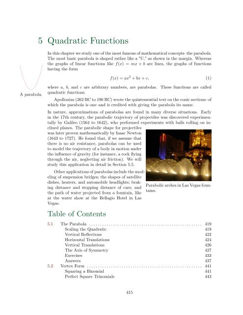
Chapter 5 Quadratic Functions - College of the Redwoods
Chapter 5 Quadratic Functions - College of the Redwoods
Chapter 5 Quadratic Functions - College of the Redwoods

Create successful ePaper yourself
Turn your PDF publications into a flip-book with our unique Google optimized e-Paper software.
5 <strong>Quadratic</strong> <strong>Functions</strong><br />
In this chapter we study one <strong>of</strong> <strong>the</strong> most famous <strong>of</strong> ma<strong>the</strong>matical concepts–<strong>the</strong> parabola.<br />
The most basic parabola is shaped ra<strong>the</strong>r like a "U," as shown in <strong>the</strong> margin. Whereas<br />
<strong>the</strong> graphs <strong>of</strong> linear functions like f(x) = mx + b are lines, <strong>the</strong> graphs <strong>of</strong> functions<br />
having <strong>the</strong> form<br />
f(x) = ax 2 + bx + c, (1)<br />
A parabola.<br />
where a, b, and c are arbitrary numbers, are parabolas.<br />
quadratic functions.<br />
These functions are called<br />
Apollonius (262 BC to 190 BC) wrote <strong>the</strong> quintessential text on <strong>the</strong> conic sections–<strong>of</strong><br />
which <strong>the</strong> parabola is one–and is credited with giving <strong>the</strong> parabola its name.<br />
In nature, approximations <strong>of</strong> parabolas are found in many diverse situations. Early<br />
in <strong>the</strong> 17th century, <strong>the</strong> parabolic trajectory <strong>of</strong> projectiles was discovered experimentally<br />
by Galileo (1564 to 1642), who performed experiments with balls rolling on inclined<br />
planes. The parabolic shape for projectiles<br />
was later proven ma<strong>the</strong>matically by Isaac Newton<br />
(1643 to 1727). He found that, if we assume that<br />
<strong>the</strong>re is no air resistance, parabolas can be used<br />
to model <strong>the</strong> trajectory <strong>of</strong> a body in motion under<br />
<strong>the</strong> influence <strong>of</strong> gravity (for instance, a rock flying<br />
through <strong>the</strong> air, neglecting air friction). We will<br />
study this application in detail in Section 5.5.<br />
O<strong>the</strong>r applications <strong>of</strong> parabolas include <strong>the</strong> modeling<br />
<strong>of</strong> suspension bridges; <strong>the</strong> shapes <strong>of</strong> satellite<br />
dishes, heaters, and automobile headlights; braking<br />
distance and stopping distance <strong>of</strong> cars; and<br />
<strong>the</strong> path <strong>of</strong> water projected from a fountain, like<br />
at <strong>the</strong> water show at <strong>the</strong> Bellagio Hotel in Las<br />
Vegas.<br />
Table <strong>of</strong> Contents<br />
Parabolic arches in Las Vegas fountains.<br />
5.1 The Parabola . . . . . . . . . . . . . . . . . . . . . . . . . . . . . . . . . . . . . . . . . . . . . . . . . . . . 419<br />
Scaling <strong>the</strong> <strong>Quadratic</strong> 419<br />
Vertical Reflections 422<br />
Horizontal Translations 424<br />
Vertical Translations 426<br />
The Axis <strong>of</strong> Symmetry 427<br />
Exercises 433<br />
Answers 437<br />
5.2 Vertex Form . . . . . . . . . . . . . . . . . . . . . . . . . . . . . . . . . . . . . . . . . . . . . . . . . . . . . 441<br />
Squaring a Binomial 441<br />
Perfect Square Trinomials 443<br />
415
416 <strong>Chapter</strong> 5 <strong>Quadratic</strong> <strong>Functions</strong><br />
Completing <strong>the</strong> Square 443<br />
Working with f(x) = x 2 + bx + c 445<br />
Working with f(x) = ax 2 + bx + c 447<br />
Exercises 453<br />
Answers 456<br />
5.3 Zeros <strong>of</strong> <strong>the</strong> <strong>Quadratic</strong> . . . . . . . . . . . . . . . . . . . . . . . . . . . . . . . . . . . . . . . . . . . . 461<br />
Factoring ax 2 + bx + c when a = 1 461<br />
Factoring ax 2 + bx + c when a ≠ 1 463<br />
Intercepts 465<br />
Putting it All Toge<strong>the</strong>r 469<br />
Exercises 473<br />
Answers 477<br />
5.4 The <strong>Quadratic</strong> Formula . . . . . . . . . . . . . . . . . . . . . . . . . . . . . . . . . . . . . . . . . . . 481<br />
Square Roots 481<br />
Development <strong>of</strong> <strong>the</strong> <strong>Quadratic</strong> Formula 483<br />
Intercepts 489<br />
The Discriminant 491<br />
Exercises 497<br />
Answers 501<br />
5.5 Motion . . . . . . . . . . . . . . . . . . . . . . . . . . . . . . . . . . . . . . . . . . . . . . . . . . . . . . . . . 505<br />
Uniform Speed 505<br />
Uniform Acceleration 507<br />
Area is Distance Traveled 510<br />
Motion in One Dimension 513<br />
The Acceleration Due to Gravity 517<br />
Exercises 521<br />
Answers 527<br />
5.6 Optimization . . . . . . . . . . . . . . . . . . . . . . . . . . . . . . . . . . . . . . . . . . . . . . . . . . . . 529<br />
Finding <strong>the</strong> Maximum or Minimum <strong>of</strong> a <strong>Quadratic</strong> Function 529<br />
A Shortcut for <strong>the</strong> Vertex 531<br />
Applications 534<br />
Exercises 541<br />
Answers 544<br />
5.7 Index . . . . . . . . . . . . . . . . . . . . . . . . . . . . . . . . . . . . . . . . . . . . . . . . . . . . . . . . . . . 545<br />
Version: Fall 2007
Section Table <strong>of</strong> Contents 417<br />
Copyright<br />
All parts <strong>of</strong> this intermediate algebra textbook are copyrighted in <strong>the</strong> name <strong>of</strong><br />
Department <strong>of</strong> Ma<strong>the</strong>matics, <strong>College</strong> <strong>of</strong> <strong>the</strong> <strong>Redwoods</strong>. They are not in <strong>the</strong> public<br />
domain. However, <strong>the</strong>y are being made available free for use in educational institutions.<br />
This <strong>of</strong>fer does not extend to any application that is made for pr<strong>of</strong>it.<br />
Users who have such applications in mind should contact David Arnold at davidarnold@redwoods.edu<br />
or Bruce Wagner at bruce-wagner@redwoods.edu.<br />
This work (including all text, Portable Document Format files, and any o<strong>the</strong>r original<br />
works), except where o<strong>the</strong>rwise noted, is licensed under a Creative Commons<br />
Attribution-NonCommercial-ShareAlike 2.5 License, and is copyrighted C○2006,<br />
Department <strong>of</strong> Ma<strong>the</strong>matics, <strong>College</strong> <strong>of</strong> <strong>the</strong> <strong>Redwoods</strong>. To view a copy <strong>of</strong> this<br />
license, visit http://creativecommons.org/licenses/by-nc-sa/2.5/ or send a letter<br />
to Creative Commons, 543 Howard Street, 5th Floor, San Francisco, California,<br />
94105, USA.<br />
Version: Fall 2007
418 <strong>Chapter</strong> 5 <strong>Quadratic</strong> <strong>Functions</strong><br />
Version: Fall 2007
Section 5.1 The Parabola 419<br />
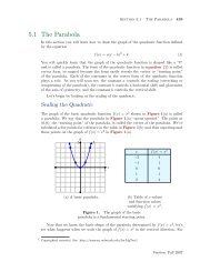
5.1 The Parabola<br />
In this section you will learn how to draw <strong>the</strong> graph <strong>of</strong> <strong>the</strong> quadratic function defined<br />
by <strong>the</strong> equation<br />
f(x) = a(x − h) 2 + k. (1)<br />
You will quickly learn that <strong>the</strong> graph <strong>of</strong> <strong>the</strong> quadratic function is shaped like a "U"<br />
and is called a parabola. The form <strong>of</strong> <strong>the</strong> quadratic function in equation (1) is called<br />
vertex form, so named because <strong>the</strong> form easily reveals <strong>the</strong> vertex or “turning point”<br />
<strong>of</strong> <strong>the</strong> parabola. Each <strong>of</strong> <strong>the</strong> constants in <strong>the</strong> vertex form <strong>of</strong> <strong>the</strong> quadratic function<br />
plays a role. As you will soon see, <strong>the</strong> constant a controls <strong>the</strong> scaling (stretching or<br />
compressing <strong>of</strong> <strong>the</strong> parabola), <strong>the</strong> constant h controls a horizontal shift and placement<br />
<strong>of</strong> <strong>the</strong> axis <strong>of</strong> symmetry, and <strong>the</strong> constant k controls <strong>the</strong> vertical shift.<br />
Let’s begin by looking at <strong>the</strong> scaling <strong>of</strong> <strong>the</strong> quadratic.<br />
Scaling <strong>the</strong> <strong>Quadratic</strong><br />
The graph <strong>of</strong> <strong>the</strong> basic quadratic function f(x) = x 2 shown in Figure 1(a) is called<br />
a parabola. We say that <strong>the</strong> parabola in Figure 1(a) “opens upward.” The point at<br />
(0, 0), <strong>the</strong> “turning point” <strong>of</strong> <strong>the</strong> parabola, is called <strong>the</strong> vertex <strong>of</strong> <strong>the</strong> parabola. We’ve<br />
tabulated a few points for reference in <strong>the</strong> table in Figure 1(b) and <strong>the</strong>n superimposed<br />
<strong>the</strong>se points on <strong>the</strong> graph <strong>of</strong> f(x) = x 2 in Figure 1(a).<br />
y<br />
5 f<br />
x<br />
5<br />
x f(x) = x 2<br />
−2 4<br />
−1 1<br />
0 0<br />
1 1<br />
2 4<br />
(a) A basic parabola.<br />
(b) Table <strong>of</strong> x-values<br />
and function values<br />
satisfying f(x) = x 2 .<br />
Figure 1. The graph <strong>of</strong> <strong>the</strong> basic<br />
parabola is a fundamental starting point.<br />
Now that we know <strong>the</strong> basic shape <strong>of</strong> <strong>the</strong> parabola determined by f(x) = x 2 , let’s<br />
see what happens when we scale <strong>the</strong> graph <strong>of</strong> f(x) = x 2 in <strong>the</strong> vertical direction. For<br />
1<br />
Copyrighted material. See: http://msenux.redwoods.edu/IntAlgText/<br />
Version: Fall 2007
420 <strong>Chapter</strong> 5 <strong>Quadratic</strong> <strong>Functions</strong><br />
example, let’s investigate <strong>the</strong> graph <strong>of</strong> g(x) = 2x 2 . The factor <strong>of</strong> 2 has a doubling<br />
effect. Note that each <strong>of</strong> <strong>the</strong> function values <strong>of</strong> g is twice <strong>the</strong> corresponding function<br />
value <strong>of</strong> f in <strong>the</strong> table in Figure 2(b).<br />
y<br />
10 g f<br />
x<br />
5<br />
x f(x) = x 2 g(x) = 2x 2<br />
−2 4 8<br />
−1 1 2<br />
0 0 0<br />
1 1 2<br />
2 4 8<br />
(a) The graphs <strong>of</strong> f and g.<br />
Figure 2.<br />
(b) Table <strong>of</strong> x-values and function values<br />
satisfying f(x) = x 2 and g(x) = 2x 2 .<br />
A stretch by a factor <strong>of</strong> 2 in <strong>the</strong> vertical direction.<br />
When <strong>the</strong> points in <strong>the</strong> table in Figure 2(b) are added to <strong>the</strong> coordinate system in<br />
Figure 2(a), <strong>the</strong> resulting graph <strong>of</strong> g is stretched by a factor <strong>of</strong> two in <strong>the</strong> vertical<br />
direction. It’s as if we had put <strong>the</strong> original graph <strong>of</strong> f on a sheet <strong>of</strong> rubber graph<br />
paper, grabbed <strong>the</strong> top and bottom edges <strong>of</strong> <strong>the</strong> sheet, and <strong>the</strong>n pulled each edge in<br />
<strong>the</strong> vertical direction to stretch <strong>the</strong> graph <strong>of</strong> f by a factor <strong>of</strong> two. Consequently, <strong>the</strong><br />
graph <strong>of</strong> g(x) = 2x 2 appears somewhat narrower in appearance, as seen in comparison<br />
to <strong>the</strong> graph <strong>of</strong> f(x) = x 2 in Figure 2(a). Note, however, that <strong>the</strong> vertex at <strong>the</strong> origin<br />
is unaffected by this scaling.<br />
In like manner, to draw <strong>the</strong> graph <strong>of</strong> h(x) = 3x 2 , take <strong>the</strong> graph <strong>of</strong> f(x) = x 2 and<br />
stretch <strong>the</strong> graph by a factor <strong>of</strong> three, tripling <strong>the</strong> y-value <strong>of</strong> each point on <strong>the</strong> original<br />
graph <strong>of</strong> f. This idea leads to <strong>the</strong> following result.<br />
Property 2. If a is a constant larger than 1, that is, if a > 1, <strong>the</strong>n <strong>the</strong> graph <strong>of</strong><br />
g(x) = ax 2 , when compared with <strong>the</strong> graph <strong>of</strong> f(x) = x 2 , is stretched by a factor<br />
<strong>of</strong> a.<br />
Version: Fall 2007
Section 5.1 The Parabola 421<br />
◮ Example 3. Compare <strong>the</strong> graphs <strong>of</strong> y = x 2 , y = 2x 2 , and y = 3x 2 on your<br />
graphing calculator.<br />
Load <strong>the</strong> functions y = x 2 , y = 2x 2 , and y = 3x 2 into <strong>the</strong> Y= menu, as shown<br />
in Figure 3(a). Push <strong>the</strong> ZOOM button and select 6:ZStandard to produce <strong>the</strong> image<br />
shown in Figure 3(b).<br />
(a)<br />
(b)<br />
Figure 3. Drawing y = x 2 , y = 2x 2 , and y = 3x 2 on <strong>the</strong><br />
graphing calculator.<br />
Note that as <strong>the</strong> “a” in y = ax 2 increases from 1 to 2 to 3, <strong>the</strong> graph <strong>of</strong> y = ax 2<br />
stretches fur<strong>the</strong>r and becomes, in a sense, narrower in appearance.<br />
Next, let’s consider what happens when we scale by a number that is smaller than<br />
1 (but greater than zero — we’ll deal with <strong>the</strong> negative in a moment). For example,<br />
let’s investigate <strong>the</strong> graph <strong>of</strong> g(x) = (1/2)x 2 . The factor 1/2 has a halving effect. Note<br />
that each <strong>of</strong> <strong>the</strong> function values <strong>of</strong> g is half <strong>the</strong> corresponding function value <strong>of</strong> f in<br />
<strong>the</strong> table in Figure 4(b).<br />
y<br />
5 f g<br />
x<br />
5<br />
x f(x) = x 2 g(x) = (1/2)x 2<br />
−2 4 2<br />
−1 1 1/2<br />
0 0 0<br />
1 1 1/2<br />
2 4 2<br />
(a) The graphs <strong>of</strong> f and g.<br />
Figure 4.<br />
(a) Table <strong>of</strong> x-values and function values<br />
satisfying f(x) = x 2 and g(x) = (1/2)x 2 .<br />
A compression by a factor <strong>of</strong> 2 in <strong>the</strong> vertical direction.<br />
When <strong>the</strong> points in <strong>the</strong> table in Figure 4(b) are added to <strong>the</strong> coordinate system<br />
in Figure 4(a), <strong>the</strong> resulting graph <strong>of</strong> g is compressed by a factor <strong>of</strong> 2 in <strong>the</strong> vertical<br />
direction. It’s as if we again placed <strong>the</strong> graph <strong>of</strong> f(x) = x 2 on a sheet <strong>of</strong> rubber graph<br />
Version: Fall 2007
422 <strong>Chapter</strong> 5 <strong>Quadratic</strong> <strong>Functions</strong><br />
paper, grabbed <strong>the</strong> top and bottom <strong>of</strong> <strong>the</strong> sheet, and <strong>the</strong>n squeezed <strong>the</strong>m toge<strong>the</strong>r by<br />
a factor <strong>of</strong> two. Consequently, <strong>the</strong> graph <strong>of</strong> g(x) = (1/2)x 2 appears somewhat wider<br />
in appearance, as seen in comparison to <strong>the</strong> graph <strong>of</strong> f(x) = x 2 in Figure 4(a). Note<br />
again that <strong>the</strong> vertex at <strong>the</strong> origin is unaffected by this scaling.<br />
Property 4. If a is a constant smaller than 1 (but larger than zero), that is,<br />
if 0 < a < 1, <strong>the</strong>n <strong>the</strong> graph <strong>of</strong> g(x) = ax 2 , when compared with <strong>the</strong> graph <strong>of</strong><br />
f(x) = x 2 , is compressed by a factor <strong>of</strong> 1/a.<br />
Some find Property 4 somewhat counterintuitive. However, if you compare <strong>the</strong><br />
function g(x) = (1/2)x 2 with <strong>the</strong> general form g(x) = ax 2 , you see that a = 1/2.<br />
Property 4 states that <strong>the</strong> graph will be compressed by a factor <strong>of</strong> 1/a. In this case,<br />
a = 1/2 and<br />
1<br />
a = 1<br />
1/2 = 2.<br />
Thus, Property 4 states that <strong>the</strong> graph <strong>of</strong> g(x) = (1/2)x 2 should be compressed by a<br />
factor <strong>of</strong> 1/(1/2) or 2, which is seen to be <strong>the</strong> case in Figure 4(a).<br />
◮ Example 5. Compare <strong>the</strong> graphs <strong>of</strong> y = x 2 , y = (1/2)x 2 , and y = (1/3)x 2 on<br />
your graphing calculator.<br />
Load <strong>the</strong> equations y = x 2 , y = (1/2)x 2 , and y = (1/3)x 2 into <strong>the</strong> Y=, as shown<br />
in Figure 5(a). Push <strong>the</strong> ZOOM button and select 6:ZStandard to produce <strong>the</strong> image<br />
shown in Figure 5(b).<br />
(a)<br />
(b)<br />
Figure 5. Drawing y = x 2 , y = (1/2)x 2 , and y = (1/3)x 2<br />
on <strong>the</strong> graphing calculator.<br />
Note that as <strong>the</strong> “a” in y = ax 2 decreases from 1 to 1/2 to 1/3, <strong>the</strong> graph <strong>of</strong> y = ax 2<br />
compresses fur<strong>the</strong>r and becomes, in a sense, wider in appearance.<br />
Vertical Reflections<br />
Let’s consider <strong>the</strong> graph <strong>of</strong> g(x) = ax 2 , when a < 0. For example, consider <strong>the</strong> graphs<br />
<strong>of</strong> g(x) = −x 2 and h(x) = (−1/2)x 2 in Figure 6.<br />
Version: Fall 2007
Section 5.1 The Parabola 423<br />
y<br />
5<br />
x<br />
5<br />
x g(x) = −x 2 h(x) = (−1/2)x 2<br />
−2 −4 −2<br />
−1 −1 −1/2<br />
0 0 0<br />
1 −1 −1/2<br />
2 −4 −2<br />
g h<br />
(a) The graphs <strong>of</strong> g and h.<br />
Figure 6.<br />
(b) Table <strong>of</strong> x-values and<br />
function values satisfying<br />
g(x) = −x 2 and h(x) = (−1/2)x 2 .<br />
A vertical reflection across <strong>the</strong> x-axis.<br />
When <strong>the</strong> table in Figure 6(b) is compared with <strong>the</strong> table in Figure 4(b), it is easy to<br />
see that <strong>the</strong> numbers in <strong>the</strong> last two columns are <strong>the</strong> same, but <strong>the</strong>y’ve been negated.<br />
The result is easy to see in Figure 6(a). The graphs have been reflected across <strong>the</strong><br />
x-axis. Each <strong>of</strong> <strong>the</strong> parabolas now “opens downward.”<br />
However, it is encouraging to see that <strong>the</strong> scaling role <strong>of</strong> <strong>the</strong> constant a in g(x) = ax 2<br />
has not changed. In <strong>the</strong> case <strong>of</strong> h(x) = (−1/2)x 2 , <strong>the</strong> y-values are still “compressed”<br />
by a factor <strong>of</strong> two, but <strong>the</strong> minus sign negates <strong>the</strong>se values, causing <strong>the</strong> graph to reflect<br />
across <strong>the</strong> x-axis. Thus, for example, one would think that <strong>the</strong> graph <strong>of</strong> y = −2x 2<br />
would be stretched by a factor <strong>of</strong> two, <strong>the</strong>n reflected across <strong>the</strong> x-axis. Indeed, this is<br />
correct, and this discussion leads to <strong>the</strong> following property.<br />
Property 6. If −1 < a < 0, <strong>the</strong>n <strong>the</strong> graph <strong>of</strong> g(x) = ax 2 , when compared with<br />
<strong>the</strong> graph <strong>of</strong> f(x) = x 2 , is compressed by a factor <strong>of</strong> 1/|a|, <strong>the</strong>n reflected across<br />
<strong>the</strong> x-axis. Secondly, if a < −1, <strong>the</strong>n <strong>the</strong> graph <strong>of</strong> g(x) = ax 2 , when compared<br />
with <strong>the</strong> graph <strong>of</strong> f(x) = x 2 , is stretched by a factor <strong>of</strong> |a|, <strong>the</strong>n reflected across<br />
<strong>the</strong> x-axis.<br />
Again, some find Property 6 confusing. However, if you compare g(x) = (−1/2)x 2<br />
with <strong>the</strong> general form g(x) = ax 2 , you see that a = −1/2. Note that in this case,<br />
−1 < a < 0. Property 6 states that <strong>the</strong> graph will be compressed by a factor <strong>of</strong> 1/|a|.<br />
In this case, a = −1/2 and<br />
1<br />
|a| = 1<br />
| − 1/2| = 2.<br />
That is, Property 6 states that <strong>the</strong> graph <strong>of</strong> g(x) = (−1/2)x 2 is compressed by a<br />
factor <strong>of</strong> 1/(| − 1/2|), or 2, <strong>the</strong>n reflected across <strong>the</strong> x-axis, which is seen to be <strong>the</strong> case<br />
in Figure 6(a). Note again that <strong>the</strong> vertex at <strong>the</strong> origin is unaffected by this scaling<br />
and reflection.<br />
Version: Fall 2007
424 <strong>Chapter</strong> 5 <strong>Quadratic</strong> <strong>Functions</strong><br />
◮ Example 7. Sketch <strong>the</strong> graphs <strong>of</strong> y = −2x 2 , y = −x 2 , and y = (−1/2)x 2 on your<br />
graphing calculator.<br />
Each <strong>of</strong> <strong>the</strong> equations were loaded separately into Y1 in <strong>the</strong> Y= menu. In each <strong>of</strong><br />
<strong>the</strong> images in Figure 7, we selected 6:ZStandard from <strong>the</strong> ZOOM menu to produce <strong>the</strong><br />
image.<br />
(a) y = −2x 2 (b) y = −x 2 (c) y = (−1/2)x 2<br />
Figure 7.<br />
In Figure 7(b), <strong>the</strong> graph <strong>of</strong> y = −x 2 is a reflection <strong>of</strong> <strong>the</strong> graph <strong>of</strong> y = x 2<br />
across <strong>the</strong> x-axis and opens downward. In Figure 7(a), note that <strong>the</strong> graph <strong>of</strong> y =<br />
−2x 2 is stretched vertically by a factor <strong>of</strong> 2 (compare with <strong>the</strong> graph <strong>of</strong> y = −x 2 in<br />
Figure 7(b)) and reflected across <strong>the</strong> x-axis to open downward. In Figure 7(c), <strong>the</strong><br />
graph <strong>of</strong> (−1/2)x 2 is compressed by a factor <strong>of</strong> 2, appears a bit wider, and is reflected<br />
across <strong>the</strong> x-axis to open downward.<br />
Horizontal Translations<br />
The graph <strong>of</strong> g(x) = (x + 1) 2 in Figure 8(a) shows a basic parabola that is shifted<br />
one unit to <strong>the</strong> left. Examine <strong>the</strong> table in Figure 8(b) and note that <strong>the</strong> equation<br />
g(x) = (x + 1) 2 produces <strong>the</strong> same y-values as does <strong>the</strong> equation f(x) = x 2 , <strong>the</strong> only<br />
difference being that <strong>the</strong>se y-values are calculated at x-values that are one unit less<br />
than those used for f(x) = x 2 . Consequently, <strong>the</strong> graph <strong>of</strong> g(x) = (x + 1) 2 must shift<br />
one unit to <strong>the</strong> left <strong>of</strong> <strong>the</strong> graph <strong>of</strong> f(x) = x 2 , as is evidenced in Figure 8(a).<br />
Note that this result is counterintuitive. One would think that replacing x with<br />
x + 1 would shift <strong>the</strong> graph one unit to <strong>the</strong> right, but <strong>the</strong> shift actually occurs in <strong>the</strong><br />
opposite direction.<br />
Finally, note that this time <strong>the</strong> vertex <strong>of</strong> <strong>the</strong> parabola has shifted 1 unit to <strong>the</strong> left<br />
and is now located at <strong>the</strong> point (−1, 0).<br />
We are led to <strong>the</strong> following conclusion.<br />
Property 8. If c > 0, <strong>the</strong>n <strong>the</strong> graph <strong>of</strong> g(x) = (x + c) 2 is shifted c units to <strong>the</strong><br />
left <strong>of</strong> <strong>the</strong> graph <strong>of</strong> f(x) = x 2 .<br />
Version: Fall 2007
Section 5.1 The Parabola 425<br />
y<br />
5 g f<br />
x<br />
5<br />
x f(x) = x 2 x g(x) = (x + 1) 2<br />
−2 4 −3 4<br />
−1 1 −2 1<br />
0 0 −1 0<br />
1 1 0 1<br />
2 4 1 4<br />
(a) The graphs <strong>of</strong> f and g.<br />
Figure 8.<br />
(a) Table <strong>of</strong> x-values and function values<br />
satisfying f(x) = x 2 and g(x) = (x + 1) 2 .<br />
A horizontal shift or translation.<br />
A similar thing happens when you replace x with x − 1, only this time <strong>the</strong> graph is<br />
shifted one unit to <strong>the</strong> right.<br />
◮ Example 9.<br />
calculator.<br />
Sketch <strong>the</strong> graphs <strong>of</strong> y = x 2 and y = (x − 1) 2 on your graphing<br />
Load <strong>the</strong> equations y = x 2 and y = (x − 1) 2 into <strong>the</strong> Y= menu, as shown in<br />
Figure 9(a). Push <strong>the</strong> ZOOM button and select 6:ZStandard to produce <strong>the</strong> image<br />
shown in Figure 9(b).<br />
Figure 9.<br />
calculator.<br />
(a)<br />
(b)<br />
Drawing y = x 2 and y = (x−1) 2 on <strong>the</strong> graphing<br />
Note that <strong>the</strong> graph <strong>of</strong> y = (x − 1) 2 is shifted 1 unit to <strong>the</strong> right <strong>of</strong> <strong>the</strong> graph <strong>of</strong> y = x 2<br />
and <strong>the</strong> vertex <strong>of</strong> <strong>the</strong> graph <strong>of</strong> y = (x − 1) 2 is now located at <strong>the</strong> point (1, 0).<br />
We are led to <strong>the</strong> following property.<br />
Property 10. If c > 0, <strong>the</strong>n <strong>the</strong> graph <strong>of</strong> g(x) = (x − c) 2 is shifted c units to<br />
<strong>the</strong> right <strong>of</strong> <strong>the</strong> graph <strong>of</strong> f(x) = x 2 .<br />
Version: Fall 2007
426 <strong>Chapter</strong> 5 <strong>Quadratic</strong> <strong>Functions</strong><br />
Vertical Translations<br />
The graph <strong>of</strong> g(x) = x 2 + 1 in Figure 10(a) is shifted one unit upward from <strong>the</strong> graph<br />
<strong>of</strong> f(x) = x 2 . This is easy to see as both equations use <strong>the</strong> same x-values in <strong>the</strong> table<br />
in Figure 10(b), but <strong>the</strong> function values <strong>of</strong> g(x) = x 2 + 1 are one unit larger than <strong>the</strong><br />
corresponding function values <strong>of</strong> f(x) = x 2 .<br />
Note that <strong>the</strong> vertex <strong>of</strong> <strong>the</strong> graph <strong>of</strong> g(x) = x 2 + 1 has also shifted upward 1 unit<br />
and is now located at <strong>the</strong> point (0, 1).<br />
y<br />
5 g f<br />
x<br />
5<br />
x f(x) = x 2 g(x) = x 2 + 1<br />
−2 4 5<br />
−1 1 2<br />
0 0 1<br />
1 1 2<br />
2 4 5<br />
Figure 10.<br />
A vertical shift or translation.<br />
The above discussion leads to <strong>the</strong> following property.<br />
Property 11. If c > 0, <strong>the</strong> graph <strong>of</strong> g(x) = x 2 + c is shifted c units upward<br />
from <strong>the</strong> graph <strong>of</strong> f(x) = x 2 .<br />
In a similar vein, <strong>the</strong> graph <strong>of</strong> y = x 2 − 1 is shifted downward one unit from <strong>the</strong><br />
graph <strong>of</strong> y = x 2 .<br />
◮ Example 12.<br />
calculator.<br />
Sketch <strong>the</strong> graphs <strong>of</strong> y = x 2 and y = x 2 − 1 on your graphing<br />
Load <strong>the</strong> equations y = x 2 and y = x 2 − 1 into <strong>the</strong> Y= menu, as shown in<br />
Figure 11(a). Push <strong>the</strong> ZOOM button and select 6:ZStandard to produce <strong>the</strong> image<br />
shown in Figure 11(b).<br />
Note that <strong>the</strong> graph <strong>of</strong> y = x 2 − 1 is shifted 1 unit downward from <strong>the</strong> graph <strong>of</strong><br />
y = x 2 and <strong>the</strong> vertex <strong>of</strong> <strong>the</strong> graph <strong>of</strong> y = x 2 − 1 is now at <strong>the</strong> point (0, −1).<br />
Version: Fall 2007
Section 5.1 The Parabola 427<br />
Figure 11.<br />
calculator.<br />
(a)<br />
(b)<br />
Drawing y = x 2 and y = x 2 −1 on <strong>the</strong> graphing<br />
The above discussion leads to <strong>the</strong> following property.<br />
Property 13. If c > 0, <strong>the</strong> graph <strong>of</strong> g(x) = x 2 − c is shifted c units downward<br />
from <strong>the</strong> graph <strong>of</strong> f(x) = x 2 .<br />
The Axis <strong>of</strong> Symmetry<br />
In Figure 1, <strong>the</strong> graph <strong>of</strong> y = x 2 is symmetric with respect to <strong>the</strong> y-axis. One half<br />
<strong>of</strong> <strong>the</strong> parabola is a mirror image <strong>of</strong> <strong>the</strong> o<strong>the</strong>r with respect to <strong>the</strong> y-axis. We say <strong>the</strong><br />
y-axis is acting as <strong>the</strong> axis <strong>of</strong> symmetry.<br />
If <strong>the</strong> parabola is reflected across <strong>the</strong> x-axis, as in Figure 6, <strong>the</strong> axis <strong>of</strong> symmetry<br />
doesn’t change. The graph is still symmetric with respect to <strong>the</strong> y-axis. Similar<br />
comments are in order for scalings and vertical translations. However, if <strong>the</strong> graph <strong>of</strong><br />
y = x 2 is shifted right or left, <strong>the</strong>n <strong>the</strong> axis <strong>of</strong> symmetry will change.<br />
◮ Example 14. Sketch <strong>the</strong> graph <strong>of</strong> y = −(x + 2) 2 + 3.<br />
Although not required, this example is much simpler if you perform reflections<br />
before translations.<br />
Tip 15.<br />
If at all possible, perform scalings and reflections before translations.<br />
In <strong>the</strong> series shown in Figure 12, we first perform a reflection, <strong>the</strong>n a horizontal<br />
translation, followed by a vertical translation.<br />
• In Figure 12(a), <strong>the</strong> graph <strong>of</strong> y = −x 2 is a reflection <strong>of</strong> <strong>the</strong> graph <strong>of</strong> y = x 2 across<br />
<strong>the</strong> x-axis and opens downward. Note that <strong>the</strong> vertex is still at <strong>the</strong> origin.<br />
• In Figure 12(b), we’ve replaced x with x+2 in <strong>the</strong> equation y = −x 2 to obtain <strong>the</strong><br />
equation y = −(x+2) 2 . The effect is to shift <strong>the</strong> graph <strong>of</strong> y = −x 2 in Figure 12(a)<br />
2 units to <strong>the</strong> left to obtain <strong>the</strong> graph <strong>of</strong> y = −(x + 2) 2 in Figure 12(b). Note that<br />
<strong>the</strong> vertex is now at <strong>the</strong> point (−2, 0).<br />
• In Figure 12(c), we’ve added 3 to <strong>the</strong> equation y = −(x+2) 2 to obtain <strong>the</strong> equation<br />
y = −(x + 2) 2 + 3. The effect is to shift <strong>the</strong> graph <strong>of</strong> y = −(x + 2) 2 in Figure 12(b)<br />
Version: Fall 2007
428 <strong>Chapter</strong> 5 <strong>Quadratic</strong> <strong>Functions</strong><br />
upward 3 units to obtain <strong>the</strong> graph <strong>of</strong> y = −(x + 2) 2 + 3 in Figure 12(c). Note<br />
that <strong>the</strong> vertex is now at <strong>the</strong> point (−2, 3).<br />
y<br />
5<br />
y<br />
5<br />
y<br />
5<br />
x<br />
5<br />
x<br />
5<br />
x<br />
5<br />
(a) y = −x 2 (b) y = −(x + 2) 2 (c) y = −(x + 2) 2 + 3<br />
Figure 12. Finding <strong>the</strong> graph <strong>of</strong> y = −(x + 2) 2 + 3<br />
through a series <strong>of</strong> transformations.<br />
In practice, we can proceed more quickly. Analyze <strong>the</strong> equation y = −(x + 2) 2 + 3.<br />
The minus sign tells us that <strong>the</strong> parabola “opens downward.” The presence <strong>of</strong> x + 2<br />
indicates a shift <strong>of</strong> 2 units to <strong>the</strong> left. Finally, adding <strong>the</strong> 3 will shift <strong>the</strong> graph 3 units<br />
upward. Thus, we have a parabola that “opens downward” with vertex at (−2, 3). This<br />
is shown in Figure 13.<br />
(−2, 3)<br />
y<br />
5<br />
x<br />
5<br />
x = −2<br />
Figure 13. The axis <strong>of</strong> symmetry<br />
passes through <strong>the</strong> vertex.<br />
The axis <strong>of</strong> symmetry passes through <strong>the</strong> vertex (−2, 3) in Figure 13 and has<br />
equation x = −2. Note that <strong>the</strong> right half <strong>of</strong> <strong>the</strong> parabola is a mirror image <strong>of</strong> its left<br />
half across this axis <strong>of</strong> symmetry. We can use <strong>the</strong> axis <strong>of</strong> symmetry to gain an accurate<br />
plot <strong>of</strong> <strong>the</strong> parabola with minimal plotting <strong>of</strong> points.<br />
Version: Fall 2007
Section 5.1 The Parabola 429<br />
Guidelines for Using <strong>the</strong> Axis <strong>of</strong> Symmetry.<br />
• Start by plotting <strong>the</strong> vertex and axis <strong>of</strong> symmetry as shown in Figure 14(a).<br />
• Next, compute two points on ei<strong>the</strong>r side <strong>of</strong> <strong>the</strong> axis <strong>of</strong> symmetry. We choose<br />
x = −1 and x = 0 and compute <strong>the</strong> corresponding y-values using <strong>the</strong> equation<br />
y = −(x + 2) 2 + 3.<br />
x y = −(x + 2) 2 + 3<br />
−1 2<br />
0 −1<br />
Plot <strong>the</strong> points from <strong>the</strong> table, as shown in Figure 14(b).<br />
• Finally, plot <strong>the</strong> mirror images <strong>of</strong> <strong>the</strong>se points across <strong>the</strong> axis <strong>of</strong> symmetry, as<br />
shown in Figure 14(c).<br />
(−2, 3)<br />
y<br />
5<br />
(−2, 3)<br />
y<br />
5<br />
(−2, 3)<br />
y<br />
5<br />
x<br />
5<br />
x<br />
5<br />
x<br />
5<br />
x = −2<br />
x = −2<br />
x = −2<br />
(a) (b) (c)<br />
Figure 14.<br />
Using <strong>the</strong> axis <strong>of</strong> symmetry to establish accuracy.<br />
The image in Figure 14(c) clearly contains enough information to complete <strong>the</strong> graph<br />
<strong>of</strong> <strong>the</strong> parabola having equation y = −(x + 2) 2 + 3 in Figure 15.<br />
(−2, 3)<br />
y<br />
5<br />
x<br />
5<br />
x = −2<br />
Figure 15. An accurate plot <strong>of</strong> y =<br />
−(x + 2) 2 + 3.<br />
Version: Fall 2007
430 <strong>Chapter</strong> 5 <strong>Quadratic</strong> <strong>Functions</strong><br />
Let’s summarize what we’ve seen thus far.<br />
Summary 16.<br />
The form <strong>of</strong> <strong>the</strong> quadratic function<br />
f(x) = a(x − h) 2 + k<br />
is called vertex form. The graph <strong>of</strong> this quadratic function is a parabola.<br />
1. The graph <strong>of</strong> <strong>the</strong> parabola opens upward if a > 0, downward if a < 0.<br />
2. If <strong>the</strong> magnitude <strong>of</strong> a is larger than 1, <strong>the</strong>n <strong>the</strong> graph <strong>of</strong> <strong>the</strong> parabola is stretched<br />
by a factor <strong>of</strong> a. If <strong>the</strong> magnitude <strong>of</strong> a is smaller than 1, <strong>the</strong>n <strong>the</strong> graph <strong>of</strong> <strong>the</strong><br />
parabola is compressed by a factor <strong>of</strong> 1/a.<br />
3. The parabola is translated h units to <strong>the</strong> right if h > 0, and h units to <strong>the</strong> left<br />
if h < 0.<br />
4. The parabola is translated k units upward if k > 0, and k units downward if<br />
k < 0.<br />
5. The coordinates <strong>of</strong> <strong>the</strong> vertex are (h, k).<br />
6. The axis <strong>of</strong> symmetry is a vertical line through <strong>the</strong> vertex whose equation is<br />
x = h.<br />
Let’s look at one final example.<br />
◮ Example 17. Use <strong>the</strong> technique <strong>of</strong> Example 14 to sketch <strong>the</strong> graph <strong>of</strong> f(x) =<br />
2(x − 2) 2 − 3.<br />
Compare f(x) = 2(x − 2) 2 − 3 with f(x) = a(x − h) 2 + k and note that a = 2.<br />
Hence, <strong>the</strong> parabola has been “stretched” by a factor <strong>of</strong> 2 and opens upward. The<br />
presence <strong>of</strong> x − 2 indicates a shift <strong>of</strong> 2 units to <strong>the</strong> right; and subtracting 3 shifts <strong>the</strong><br />
parabola 3 units downward. Therefore, <strong>the</strong> vertex will be located at <strong>the</strong> point (2, −3)<br />
and <strong>the</strong> axis <strong>of</strong> symmetry will be <strong>the</strong> vertical line having equation x = 2. This is shown<br />
in Figure 16(a).<br />
Note. Some prefer a more strict comparison <strong>of</strong> f(x) = 2(x − 2) 2 − 3 with <strong>the</strong><br />
general vertex form f(x) = a(x − h) 2 + k, yielding a = 2, h = 2, and k = −3. This<br />
immediately identifies <strong>the</strong> vertex at (h, k), or (2, −3).<br />
Next, evaluate <strong>the</strong> function f(x) = 2(x − 2) 2 − 3 at two points lying to <strong>the</strong> right <strong>of</strong><br />
<strong>the</strong> axis <strong>of</strong> symmetry (or to <strong>the</strong> left, if you prefer). Because <strong>the</strong> axis <strong>of</strong> symmetry is<br />
<strong>the</strong> vertical line x = 2, we choose to evaluate <strong>the</strong> function at x = 3 and 4.<br />
f(3) = 2(3 − 2) 2 − 3 = −1<br />
f(4) = 2(4 − 2) 2 − 3 = 5<br />
This gives us two points to <strong>the</strong> right <strong>of</strong> <strong>the</strong> axis <strong>of</strong> symmetry, (3, −1) and (4, 5), which<br />
we plot in Figure 16(b).<br />
Finally, we plot <strong>the</strong> mirror images <strong>of</strong> (3, −1) and (4, 5) across <strong>the</strong> axis <strong>of</strong> symmetry,<br />
which gives us <strong>the</strong> points (1, −1) and (0, 5), respectively. These are plotted in<br />
Figure 16(c). We <strong>the</strong>n draw <strong>the</strong> parabola through <strong>the</strong>se points.<br />
Version: Fall 2007
Section 5.1 The Parabola 431<br />
y<br />
5<br />
y<br />
5<br />
y<br />
5<br />
f<br />
x<br />
5<br />
x<br />
5<br />
x<br />
5<br />
(2, −3)<br />
(2, −3)<br />
(2, −3)<br />
x = 2<br />
x = 2<br />
x = 2<br />
(a) (b) (c)<br />
Figure 16. Creating <strong>the</strong> graph <strong>of</strong> f(x) = 2(x − 2) 2 − 3.<br />
Let’s finish by describing <strong>the</strong> domain and range <strong>of</strong> <strong>the</strong> function defined by <strong>the</strong><br />
rule f(x) = 2(x − 2) 2 − 3. If you use <strong>the</strong> intuitive notion that <strong>the</strong> domain is <strong>the</strong> set <strong>of</strong><br />
“permissible x-values,” <strong>the</strong>n one can substitute any number one wants into <strong>the</strong> equation<br />
f(x) = 2(x − 2) 2 − 3. Therefore, <strong>the</strong> domain is all real numbers, which we can write as<br />
follows: Domain = R or Domain = (−∞, ∞).<br />
You can also project each point on <strong>the</strong> graph <strong>of</strong> f(x) = 2(x−2) 2 −3 onto <strong>the</strong> x-axis,<br />
as shown in Figure 17(a). If you do this, <strong>the</strong>n <strong>the</strong> entire axis will “lie in shadow,” so<br />
once again, <strong>the</strong> domain is all real numbers.<br />
y<br />
5<br />
y<br />
5<br />
x<br />
5<br />
x<br />
5<br />
−3<br />
(a)<br />
(b)<br />
Figure 17. Projecting to find<br />
(a) <strong>the</strong> domain and (b) <strong>the</strong> range.<br />
To determine <strong>the</strong> range <strong>of</strong> <strong>the</strong> function f(x) = 2(x − 2) 2 − 3, project each point<br />
on <strong>the</strong> graph <strong>of</strong> f onto <strong>the</strong> y-axis, as shown in Figure 17(b). On <strong>the</strong> y-axis, all<br />
points greater than or equal to −3 “lie in shadow,” so <strong>the</strong> range is described with<br />
Range = {y : y ≥ −3} = [−3, ∞).<br />
Version: Fall 2007
432 <strong>Chapter</strong> 5 <strong>Quadratic</strong> <strong>Functions</strong><br />
The following summarizes how one finds <strong>the</strong> domain and range <strong>of</strong> a quadratic function<br />
that is in vertex form.<br />
Summary 18.<br />
The domain <strong>of</strong> <strong>the</strong> quadratic function<br />
f(x) = a(x − h) 2 + k,<br />
regardless <strong>of</strong> <strong>the</strong> values <strong>of</strong> <strong>the</strong> parameters a, h, and k, is <strong>the</strong> set <strong>of</strong> all real numbers,<br />
easily described with R or (−∞, ∞). On <strong>the</strong> o<strong>the</strong>r hand, <strong>the</strong> range depends upon<br />
<strong>the</strong> values <strong>of</strong> a and k.<br />
• If a > 0, <strong>the</strong>n <strong>the</strong> parabola opens upward and has vertex at (h, k). Consequently,<br />
<strong>the</strong> range will be<br />
[k, ∞) = {y : y ≥ k}.<br />
• If a < 0, <strong>the</strong>n <strong>the</strong> parabola opens downward and has vertex at (h, k). Consequently,<br />
<strong>the</strong> range will be<br />
(−∞, k] = {y : y ≤ k}.<br />
Version: Fall 2007
Section 5.1 The Parabola 433<br />
5.1 Exercises<br />
In Exercises 1-6, sketch <strong>the</strong> image <strong>of</strong><br />
your calculator screen on your homework<br />
paper. Label and scale each axis with<br />
xmin, xmax, ymin, and ymax. Label<br />
each graph with its equation. Remember<br />
to use a ruler to draw all lines, including<br />
axes.<br />
1. Use your graphing calculator to sketch<br />
<strong>the</strong> graphs <strong>of</strong> f(x) = x 2 , g(x) = 2x 2 , and<br />
h(x) = 4x 2 on one screen. Write a short<br />
sentence explaining what you learned in<br />
this exercise.<br />
2. Use your graphing calculator to sketch<br />
<strong>the</strong> graphs <strong>of</strong> f(x) = −x 2 , g(x) = −2x 2 ,<br />
and h(x) = −4x 2 on one screen. Write a<br />
short sentence explaining what you learned<br />
in this exercise.<br />
3. Use your graphing calculator to sketch<br />
<strong>the</strong> graphs <strong>of</strong> f(x) = x 2 , g(x) = (x −<br />
2) 2 , and h(x) = (x − 4) 2 on one screen.<br />
Write a short sentence explaining what<br />
you learned in this exercise.<br />
4. Use your graphing calculator to sketch<br />
<strong>the</strong> graphs <strong>of</strong> f(x) = x 2 , g(x) = (x +<br />
2) 2 , and h(x) = (x + 4) 2 on one screen.<br />
Write a short sentence explaining what<br />
you learned in this exercise.<br />
5. Use your graphing calculator to sketch<br />
<strong>the</strong> graphs <strong>of</strong> f(x) = x 2 , g(x) = x 2 +<br />
2, and h(x) = x 2 + 4 on one screen.<br />
Write a short sentence explaining what<br />
you learned in this exercise.<br />
6. Use your graphing calculator to sketch<br />
<strong>the</strong> graphs <strong>of</strong> f(x) = x 2 , g(x) = x 2 −<br />
2, and h(x) = x 2 − 4 on one screen.<br />
Write a short sentence explaining what<br />
you learned in this exercise.<br />
In Exercises 7-14, write down <strong>the</strong> given<br />
quadratic function on your homework paper,<br />
<strong>the</strong>n state <strong>the</strong> coordinates <strong>of</strong> <strong>the</strong> vertex.<br />
7. f(x) = −5(x − 4) 2 − 5<br />
8. f(x) = 5(x + 3) 2 − 7<br />
9. f(x) = 3(x + 1) 2<br />
10. f(x) = 7 5<br />
(<br />
x + 5 ) 2<br />
− 3 9 4<br />
11. f(x) = −7(x − 4) 2 + 6<br />
12. f(x) = − 1 2<br />
13. f(x) = 1 6<br />
14. f(x) = − 3 2<br />
(<br />
x − 8 ) 2<br />
+ 2 9 9<br />
(<br />
x + 7 ) 2<br />
+ 3 3 8<br />
(<br />
x + 1 ) 2<br />
− 8 2 9<br />
In Exercises 15-22, state <strong>the</strong> equation<br />
<strong>of</strong> <strong>the</strong> axis <strong>of</strong> symmetry <strong>of</strong> <strong>the</strong> graph <strong>of</strong><br />
<strong>the</strong> given quadratic function.<br />
15. f(x) = −7(x − 3) 2 + 1<br />
16. f(x) = −6(x + 8) 2 + 1<br />
2<br />
Copyrighted material. See: http://msenux.redwoods.edu/IntAlgText/<br />
Version: Fall 2007
434 <strong>Chapter</strong> 5 <strong>Quadratic</strong> <strong>Functions</strong><br />
17. f(x) = − 7 8<br />
18. f(x) = − 1 2<br />
19. f(x) = − 2 9<br />
(<br />
x + 1 ) 2<br />
+ 2 4 3<br />
(<br />
x − 3 ) 2<br />
− 5 8 7<br />
(<br />
x + 2 ) 2<br />
− 4 3 5<br />
20. f(x) = −7(x + 3) 2 + 9<br />
21. f(x) = − 8 7<br />
(<br />
x + 2 ) 2<br />
+ 6 9 5<br />
22. f(x) = 3(x + 3) 2 + 6<br />
In Exercises 23-36, perform each <strong>of</strong> <strong>the</strong><br />
following tasks for <strong>the</strong> given quadratic<br />
function.<br />
i. Set up a coordinate system on graph<br />
paper. Label and scale each axis.<br />
ii. Plot <strong>the</strong> vertex <strong>of</strong> <strong>the</strong> parabola and<br />
label it with its coordinates.<br />
iii. Draw <strong>the</strong> axis <strong>of</strong> symmetry and label<br />
it with its equation.<br />
iv. Set up a table near your coordinate<br />
system that contains exact coordinates<br />
<strong>of</strong> two points on ei<strong>the</strong>r side <strong>of</strong> <strong>the</strong> axis<br />
<strong>of</strong> symmetry. Plot <strong>the</strong>m on your coordinate<br />
system and <strong>the</strong>ir “mirror images”<br />
across <strong>the</strong> axis <strong>of</strong> symmetry.<br />
v. Sketch <strong>the</strong> parabola and label it with<br />
its equation.<br />
vi. Use interval notation to describe both<br />
<strong>the</strong> domain and range <strong>of</strong> <strong>the</strong> quadratic<br />
function.<br />
23. f(x) = (x + 2) 2 − 3<br />
24. f(x) = (x − 3) 2 − 4<br />
27. f(x) = (x − 3) 2<br />
28. f(x) = −(x + 2) 2<br />
29. f(x) = −x 2 + 7<br />
30. f(x) = −x 2 + 7<br />
31. f(x) = 2(x − 1) 2 − 6<br />
32. f(x) = −2(x + 1) 2 + 5<br />
33. f(x) = − 1 2 (x + 1)2 + 5<br />
34. f(x) = 1 2 (x − 3)2 − 6<br />
35. f(x) = 2(x − 5/2) 2 − 15/2<br />
36. f(x) = −3(x + 7/2) 2 + 15/4<br />
In Exercises 37-44, write <strong>the</strong> given quadratic<br />
function on your homework paper,<br />
<strong>the</strong>n use set-builder and interval notation<br />
to describe <strong>the</strong> domain and <strong>the</strong><br />
range <strong>of</strong> <strong>the</strong> function.<br />
37. f(x) = 7(x + 6) 2 − 6<br />
38. f(x) = 8(x + 1) 2 + 7<br />
39. f(x) = −3(x + 4) 2 − 7<br />
40. f(x) = −6(x − 7) 2 + 9<br />
41. f(x) = −7(x + 5) 2 − 7<br />
42. f(x) = 8(x − 4) 2 + 3<br />
43. f(x) = −4(x − 1) 2 + 2<br />
44. f(x) = 7(x − 2) 2 − 3<br />
25. f(x) = −(x − 2) 2 + 5<br />
26. f(x) = −(x + 4) 2 + 4<br />
Version: Fall 2007
Section 5.1 The Parabola 435<br />
In Exercises 45-52, using <strong>the</strong> given value<br />
<strong>of</strong> a, find <strong>the</strong> specific quadratic function<br />
<strong>of</strong> <strong>the</strong> form f(x) = a(x − h) 2 + k that<br />
has <strong>the</strong> graph shown. Note: h and k are<br />
integers. Check your solution with your<br />
graphing calculator.<br />
45. a = −2<br />
y<br />
5<br />
48. a = 0.5<br />
y<br />
5<br />
x<br />
5<br />
x<br />
5<br />
49. a = 2<br />
y<br />
5<br />
46. a = 0.5<br />
y<br />
5<br />
x<br />
5<br />
x<br />
5<br />
50. a = −0.5<br />
y<br />
5<br />
47. a = 2<br />
y<br />
5<br />
x<br />
5<br />
x<br />
5<br />
Version: Fall 2007
436 <strong>Chapter</strong> 5 <strong>Quadratic</strong> <strong>Functions</strong><br />
51. a = 2<br />
y<br />
5<br />
54.<br />
y<br />
5<br />
x<br />
5<br />
x<br />
5<br />
52. a = 0.5<br />
y<br />
5<br />
x<br />
5<br />
In Exercises 55-56, use <strong>the</strong> graph to<br />
determine <strong>the</strong> domain <strong>of</strong> <strong>the</strong> function f(x) =<br />
ax 2 +bx+c. The arrows on <strong>the</strong> graph are<br />
meant to indicate that <strong>the</strong> graph continues<br />
indefinitely in <strong>the</strong> continuing pattern<br />
and direction <strong>of</strong> each arrow. Use interval<br />
notation to describe your solution.<br />
55.<br />
y<br />
5<br />
In Exercises 53-54, use <strong>the</strong> graph to<br />
determine <strong>the</strong> range <strong>of</strong> <strong>the</strong> function f(x) =<br />
ax 2 +bx+c. The arrows on <strong>the</strong> graph are<br />
meant to indicate that <strong>the</strong> graph continues<br />
indefinitely in <strong>the</strong> continuing pattern<br />
and direction <strong>of</strong> each arrow. Describe<br />
your solution using interval notation.<br />
x<br />
5<br />
53.<br />
y<br />
5<br />
56.<br />
y<br />
5<br />
x<br />
5<br />
x<br />
5<br />
Version: Fall 2007
Section 5.1 The Parabola 437<br />
5.1 Answers<br />
1. Multiplying by 2 scales vertically by<br />
a factor <strong>of</strong> 2. Multiplying by 4 scales<br />
vertically by a factor <strong>of</strong> 4.<br />
y<br />
10<br />
hg f<br />
5. The graph <strong>of</strong> g(x) = x 2 +2 is shifted<br />
2 units to <strong>the</strong> upward from <strong>the</strong> graph <strong>of</strong><br />
f(x) = x 2 . The graph <strong>of</strong> h(x) = x 2 + 4<br />
is shifted 4 units upward from <strong>the</strong> graph<br />
<strong>of</strong> f(x) = x 2 .<br />
y<br />
10<br />
x<br />
10<br />
h<br />
g<br />
f<br />
x<br />
10<br />
3. The graph <strong>of</strong> g(x) = (x−2) 2 is shifted<br />
2 units to <strong>the</strong> right <strong>of</strong> f(x) = x 2 . The<br />
graph <strong>of</strong> h(x) = (x−4) 2 is shifted 4 units<br />
to <strong>the</strong> right <strong>of</strong> f(x) = x 2 .<br />
y<br />
10<br />
f g h<br />
7. (4, −5)<br />
9. (−1, 0)<br />
11. (4, 6)<br />
13.<br />
(<br />
− 7 3 , 3 )<br />
8<br />
x<br />
10<br />
15. x = 3<br />
17. x = − 1 4<br />
19. x = − 2 3<br />
21. x = − 2 9<br />
Version: Fall 2007
438 <strong>Chapter</strong> 5 <strong>Quadratic</strong> <strong>Functions</strong><br />
29. Domain= (−∞, ∞); Range= (−∞, 7]<br />
23. Domain= (−∞, ∞); Range= [−3, ∞)<br />
y<br />
10<br />
f(x)=(x−3) 2 y<br />
10<br />
y<br />
10 f(x)=(x+2) 2 −3<br />
y<br />
10<br />
(0,7)<br />
x<br />
10<br />
x<br />
10<br />
(−2,−3)<br />
x=−2<br />
f(x)=−x 2 +7<br />
x=0<br />
25. Domain= (−∞, ∞); Range= (−∞, 5] 31. Domain= (−∞, ∞); Range= [−6, ∞)<br />
y<br />
10<br />
y<br />
10 f(x)=2(x−1) 2 −6<br />
(2,5)<br />
x<br />
10<br />
x<br />
10<br />
(1,−6)<br />
f(x)=−(x−2) 2 +5<br />
x=2<br />
x=1<br />
27. Domain= (−∞, ∞); Range= [0, ∞) 33. Domain= (−∞, ∞); Range= (−∞, 5]<br />
(−1,5)<br />
(3,0)<br />
x<br />
10<br />
x<br />
10<br />
x=3<br />
x=−1<br />
f(x)=− 1 2 (x+1)2 +5<br />
Version: Fall 2007
Section 5.1 The Parabola 439<br />
35. Domain= (−∞, ∞); Range= [−15/2, ∞)<br />
y<br />
10<br />
f(x)=2(x−5/2) 2 −15/2<br />
x<br />
10<br />
x=5/2<br />
(5/2,−15/2)<br />
37. Domain= (−∞, ∞); Range= [−6, ∞) =<br />
{y : y ≥ −6}<br />
39. Domain= (−∞, ∞); Range= (−∞, −7] =<br />
{y : y ≤ −7}<br />
41. Domain= (−∞, ∞); Range= (−∞, −7] =<br />
{y : y ≤ −7}<br />
43. Domain= (−∞, ∞); Range= (−∞, 2] =<br />
{y : y ≤ 2}<br />
45. f(x) = −2(x − 3) 2 + 1<br />
47. f(x) = 2(x + 1) 2 − 1<br />
49. f(x) = 2(x + 2) 2 + 1<br />
51. f(x) = 2(x − 3) 2 − 1<br />
53. (−∞, −2]<br />
55. (−∞, ∞)<br />
Version: Fall 2007
440 <strong>Chapter</strong> 5 <strong>Quadratic</strong> <strong>Functions</strong><br />
Version: Fall 2007
Section 5.2 Vertex Form 441<br />
5.2 Vertex Form<br />
In <strong>the</strong> previous section, you learned that it is a simple task to sketch <strong>the</strong> graph <strong>of</strong> a<br />
quadratic function if it is presented in vertex form<br />
f(x) = a(x − h) 2 + k. (1)<br />
The goal <strong>of</strong> <strong>the</strong> current section is to start with <strong>the</strong> most general form <strong>of</strong> <strong>the</strong> quadratic<br />
function, namely<br />
f(x) = ax 2 + bx + c, (2)<br />
and manipulate <strong>the</strong> equation into vertex form. Once you have your quadratic function<br />
in vertex form, <strong>the</strong> technique <strong>of</strong> <strong>the</strong> previous section should allow you to construct <strong>the</strong><br />
graph <strong>of</strong> <strong>the</strong> quadratic function.<br />
However, before we turn our attention to <strong>the</strong> task <strong>of</strong> converting <strong>the</strong> general quadratic<br />
into vertex form, we need to review <strong>the</strong> necessary algebraic fundamentals. Let’s begin<br />
with a review <strong>of</strong> an important algebraic shortcut called squaring a binomial.<br />
Squaring a Binomial<br />
A monomial is a single algebraic term, usually constructed as a product <strong>of</strong> a number<br />
(called a coefficient) and one or more variables raised to nonnegative integral powers,<br />
such as −3x 2 or 14y 3 z 5 . The key phrase here is “single term.” A binomial is an algebraic<br />
sum or difference <strong>of</strong> two monomials (or terms), such as x + 2y or 3ab 2 − 2c 3 . The key<br />
phrase here is “two terms.”<br />
To “square a binomial,” start with an arbitrary binomial, such as a+b, <strong>the</strong>n multiply<br />
it by itself to produce its square (a + b)(a + b), or, more compactly, (a + b) 2 . We can<br />
use <strong>the</strong> distributive property to expand <strong>the</strong> square <strong>of</strong> <strong>the</strong> binomial a + b.<br />
(a + b) 2 = (a + b)(a + b)<br />
= a(a + b) + b(a + b)<br />
= a 2 + ab + ba + b 2<br />
Because ab = ba, we can add <strong>the</strong> two middle terms to arrive at <strong>the</strong> following property.<br />
Property 3.<br />
The square <strong>of</strong> <strong>the</strong> binomial a + b is expanded as follows.<br />
(a + b) 2 = a 2 + 2ab + b 2 (4)<br />
3<br />
Copyrighted material. See: http://msenux.redwoods.edu/IntAlgText/<br />
Version: Fall 2007
442 <strong>Chapter</strong> 5 <strong>Quadratic</strong> <strong>Functions</strong><br />
◮ Example 5. Expand (x + 4) 2 .<br />
We could proceed as follows.<br />
(x + 4) 2 = (x + 4)(x + 4)<br />
= x(x + 4) + 4(x + 4)<br />
= x 2 + 4x + 4x + 16<br />
= x 2 + 8x + 16<br />
Although correct, this technique will not help us with our upcoming task. What<br />
we need to do is follow <strong>the</strong> algorithm suggested by Property 3.<br />
Algorithm for Squaring a Binomial. To square <strong>the</strong> binomial a + b, proceed<br />
as follows:<br />
1. Square <strong>the</strong> first term to get a 2 .<br />
2. Multiply <strong>the</strong> first and second terms toge<strong>the</strong>r, and <strong>the</strong>n multiply <strong>the</strong> result by<br />
two to get 2ab.<br />
3. Square <strong>the</strong> second term to get b 2 .<br />
Thus, to expand (x + 4) 2 , we should proceed as follows.<br />
1. Square <strong>the</strong> first term to get x 2<br />
2. Multiply <strong>the</strong> first and second terms toge<strong>the</strong>r and <strong>the</strong>n multiply by two to get 8x.<br />
3. Square <strong>the</strong> second term to get 16.<br />
Proceeding in this manner allows us to perform <strong>the</strong> expansion mentally and simply<br />
write down <strong>the</strong> solution.<br />
(x + 4) 2 = x 2 + 2(x)(4) + 4 2 = x 2 + 8x + 16<br />
Here are a few more examples. In each, we’ve written an extra step to help clarify<br />
<strong>the</strong> procedure. In practice, you should simply write down <strong>the</strong> solution without any<br />
intermediate steps.<br />
(x + 3) 2 = x 2 + 2(x)(3) + 3 2 = x 2 + 6x + 9<br />
(x − 5) 2 = x 2 + 2(x)(−5) + (−5) 2 = x 2 − 10x + 25<br />
(<br />
x −<br />
1 2<br />
2)<br />
= x 2 + 2(x) ( − 1 ) (<br />
2 + −<br />
1 2<br />
2)<br />
= x 2 − x + 1 4<br />
It is imperative that you master this shortcut before moving on to <strong>the</strong> rest <strong>of</strong> <strong>the</strong><br />
material in this section.<br />
Version: Fall 2007
Section 5.2 Vertex Form 443<br />
Perfect Square Trinomials<br />
Once you’ve mastered squaring a binomial, as in<br />
(a + b) 2 = a 2 + 2ab + b 2 , (6)<br />
it’s a simple matter to identify and factor trinomials (three terms) having <strong>the</strong> form<br />
a 2 + 2ab + b 2 . You simply “undo” <strong>the</strong> multiplication. Whenever you spot a trinomial<br />
whose first and third terms are perfect squares, you should suspect that it factors as<br />
follows.<br />
a 2 + 2ab + b 2 = (a + b) 2 (7)<br />
A trinomial that factors according to this rule or pattern is called a perfect square<br />
trinomial.<br />
For example, <strong>the</strong> first and last terms <strong>of</strong> <strong>the</strong> following trinomial are perfect squares.<br />
x 2 + 16x + 64<br />
The square roots <strong>of</strong> <strong>the</strong> first and last terms are x and 8, respectively. Hence, it makes<br />
sense to try <strong>the</strong> following.<br />
x 2 + 16x + 64 = (x + 8) 2<br />
It is important that you check your result using multiplication. So, following <strong>the</strong><br />
three-step algorithm for squaring a binomial:<br />
1. Square x to get x 2 .<br />
2. Multiply x and 8 to get 8x, <strong>the</strong>n multiply this result by 2 to get 16x.<br />
3. Square 8 to get 64.<br />
Hence, x 2 + 16x + 64 is a perfect square trinomial and factors as (x + 8) 2 .<br />
As ano<strong>the</strong>r example, consider x 2 − 10x + 25. The square roots <strong>of</strong> <strong>the</strong> first and last<br />
terms are x and 5, respectively. Hence, it makes sense to try<br />
x 2 − 10x + 25 = (x − 5) 2 .<br />
Again, you should check this result. Note especially that twice <strong>the</strong> product <strong>of</strong> x and<br />
−5 equals <strong>the</strong> middle term on <strong>the</strong> left, namely, −10x.<br />
Completing <strong>the</strong> Square<br />
If a quadratic function is given in vertex form, it is a simple matter to sketch <strong>the</strong><br />
parabola represented by <strong>the</strong> equation. For example, consider <strong>the</strong> quadratic function<br />
f(x) = (x + 2) 2 + 3,<br />
which is in vertex form. The graph <strong>of</strong> this equation is a parabola that opens upward.<br />
It is translated 2 units to <strong>the</strong> left and 3 units upward. This is <strong>the</strong> advantage <strong>of</strong> vertex<br />
Version: Fall 2007
444 <strong>Chapter</strong> 5 <strong>Quadratic</strong> <strong>Functions</strong><br />
form. The transformations required to draw <strong>the</strong> graph <strong>of</strong> <strong>the</strong> function are easy to spot<br />
when <strong>the</strong> equation is written in vertex form.<br />
It’s a simple matter to transform <strong>the</strong> equation f(x) = (x + 2) 2 + 3 into <strong>the</strong> general<br />
form <strong>of</strong> a quadratic function, f(x) = ax 2 + bx + c. We simply use <strong>the</strong> three-step<br />
algorithm to square <strong>the</strong> binomial; <strong>the</strong>n we combine like terms.<br />
f(x) = (x + 2) 2 + 3<br />
f(x) = x 2 + 4x + 4 + 3<br />
f(x) = x 2 + 4x + 7<br />
Note, however, that <strong>the</strong> result <strong>of</strong> this manipulation, f(x) = x 2 + 4x + 7, is not as useful<br />
as vertex form, as it is difficult to identify <strong>the</strong> transformations required to draw <strong>the</strong><br />
parabola represented by <strong>the</strong> equation f(x) = x 2 + 4x + 7.<br />
It’s really <strong>the</strong> reverse <strong>of</strong> <strong>the</strong> manipulation above that is needed. If we are presented<br />
with an equation in <strong>the</strong> form f(x) = ax 2 + bx + c, such as f(x) = x 2 + 4x + 7, <strong>the</strong>n an<br />
algebraic method is needed to convert this equation to vertex form f(x) = a(x−h) 2 +k;<br />
or in this case, back to its original vertex form f(x) = (x + 2) 2 + 3.<br />
The procedure we seek is called completing <strong>the</strong> square. The name is derived from<br />
<strong>the</strong> fact that we need to “complete” <strong>the</strong> trinomial on <strong>the</strong> right side <strong>of</strong> y = x 2 + 4x + 7<br />
so that it becomes a perfect square trinomial.<br />
Algorithm for Completing <strong>the</strong> Square The procedure for completing <strong>the</strong><br />
square involves three key steps.<br />
1. Take half <strong>of</strong> <strong>the</strong> coefficient <strong>of</strong> x and square <strong>the</strong> result.<br />
2. Add and subtract <strong>the</strong> quantity from step one so that <strong>the</strong> right-hand side <strong>of</strong> <strong>the</strong><br />
equation does not change.<br />
3. Factor <strong>the</strong> resulting perfect square trinomial and combine constant terms.<br />
Let’s follow this procedure and place f(x) = x 2 + 4x + 7 in vertex form.<br />
1. Take half <strong>of</strong> <strong>the</strong> coefficient <strong>of</strong> x. Thus, (1/2)(4) = 2. Square this result. Thus,<br />
2 2 = 4.<br />
2. Add and subtract 4 on <strong>the</strong> right side <strong>of</strong> <strong>the</strong> equation f(x) = x 2 + 4x + 7.<br />
f(x) = x 2 + 4x + 4 − 4 + 7<br />
3. Group <strong>the</strong> first three terms on <strong>the</strong> right-hand side. These form a perfect square<br />
trinomial.<br />
f(x) = (x 2 + 4x + 4) − 4 + 7<br />
Now factor <strong>the</strong> perfect square trinomial and combine <strong>the</strong> constants at <strong>the</strong> end to<br />
get<br />
f(x) = (x + 2) 2 + 3.<br />
Version: Fall 2007
Section 5.2 Vertex Form 445<br />
That’s it, we’re done! We’ve returned <strong>the</strong> general quadratic f(x) = x 2 + 4x + 7<br />
back to vertex form f(x) = (x + 2) 2 + 3.<br />
Let’s try that once more.<br />
◮ Example 8.<br />
Place <strong>the</strong> quadratic function f(x) = x 2 − 8x − 9 in vertex form.<br />
We follow <strong>the</strong> three-step algorithm for completing <strong>the</strong> square.<br />
1. Take half <strong>of</strong> <strong>the</strong> coefficient <strong>of</strong> x and square: i.e.,<br />
[(1/2)(−8)] 2 = [−4] 2 = 16.<br />
2. Add and subtract this amount to <strong>the</strong> right-hand side <strong>of</strong> <strong>the</strong> function.<br />
f(x) = x 2 − 8x + 16 − 16 − 9<br />
3. Group <strong>the</strong> first three terms on <strong>the</strong> right-hand side. These form a perfect square<br />
trinomial.<br />
f(x) = (x 2 − 8x + 16) − 16 − 9<br />
Factor <strong>the</strong> perfect square trinomial and combine <strong>the</strong> coefficients at <strong>the</strong> end.<br />
f(x) = (x − 4) 2 − 25<br />
Now, let’s see how we can use <strong>the</strong> technique <strong>of</strong> completing <strong>the</strong> square to help in<br />
drawing <strong>the</strong> graphs <strong>of</strong> general quadratic functions.<br />
Working with f(x) = x 2 + bx + c<br />
The examples in this section will have <strong>the</strong> form f(x) = x 2 + bx + c. Note that <strong>the</strong><br />
coefficient <strong>of</strong> x 2 is 1. In <strong>the</strong> next section, we will work with a harder form, f(x) =<br />
ax 2 + bx + c, where a ≠ 1.<br />
◮ Example 9.<br />
sketch its graph.<br />
Complete <strong>the</strong> square to place f(x) = x 2 + 6x + 2 in vertex form and<br />
First, take half <strong>of</strong> <strong>the</strong> coefficient <strong>of</strong> x and square; i.e., [(1/2)(6)] 2 = 9. On <strong>the</strong> right<br />
side <strong>of</strong> <strong>the</strong> equation, add and subtract this amount so as to not change <strong>the</strong> equation.<br />
f(x) = x 2 + 6x + 9 − 9 + 2<br />
Group <strong>the</strong> first three terms on <strong>the</strong> right-hand side.<br />
f(x) = (x 2 + 6x + 9) − 9 + 2<br />
The first three terms on <strong>the</strong> right-hand side form a perfect square trinomial that is<br />
easily factored. Also, combine <strong>the</strong> constants at <strong>the</strong> end.<br />
f(x) = (x + 3) 2 − 7<br />
Version: Fall 2007
446 <strong>Chapter</strong> 5 <strong>Quadratic</strong> <strong>Functions</strong><br />
This is a parabola that opens upward. We need to shift <strong>the</strong> parabola 3 units to <strong>the</strong> left<br />
and <strong>the</strong>n 7 units downward, placing <strong>the</strong> vertex at (−3, −7) as shown in Figure 1(a).<br />
The axis <strong>of</strong> symmetry is <strong>the</strong> vertical line x = −3. The table in Figure 1(b) calculates<br />
two points to <strong>the</strong> right <strong>of</strong> <strong>the</strong> axis <strong>of</strong> symmetry, and mirror points on <strong>the</strong> left <strong>of</strong> <strong>the</strong><br />
axis <strong>of</strong> symmetry make for an accurate plot <strong>of</strong> <strong>the</strong> parabola.<br />
y<br />
10<br />
x<br />
10<br />
x y = (x + 3) 2 − 7<br />
−2 −6<br />
−1 −3<br />
(−3, −7)<br />
x = −3<br />
(a)<br />
(b)<br />
Figure 1. Plotting <strong>the</strong> graph <strong>of</strong> <strong>the</strong><br />
quadratic function f(x) = (x + 3) 2 − 7.<br />
Let’s look at ano<strong>the</strong>r example.<br />
◮ Example 10. Complete <strong>the</strong> square to place f(x) = x 2 − 8x + 21 in vertex form<br />
and sketch its graph.<br />
First, take half <strong>of</strong> <strong>the</strong> coefficient <strong>of</strong> x and square; i.e., [(1/2)(−8)] 2 = 16. On<br />
<strong>the</strong> right side <strong>of</strong> <strong>the</strong> equation, add and subtract this amount so as to not change <strong>the</strong><br />
equation.<br />
f(x) = x 2 − 8x + 16 − 16 + 21<br />
Group <strong>the</strong> first three terms on <strong>the</strong> right-hand side <strong>of</strong> <strong>the</strong> equation.<br />
f(x) = (x 2 − 8x + 16) − 16 + 21<br />
The first three terms form a perfect square trinomial that is easily factored.<br />
combine constants at <strong>the</strong> end.<br />
Also,<br />
f(x) = (x − 4) 2 + 5<br />
This is a parabola that opens upward. We need to shift <strong>the</strong> parabola 4 units to <strong>the</strong><br />
right and <strong>the</strong>n 5 units upward, placing <strong>the</strong> vertex at (4, 5), as shown in Figure 2(a).<br />
The table in Figure 2(b) calculates two points to <strong>the</strong> right <strong>of</strong> <strong>the</strong> axis <strong>of</strong> symmetry,<br />
and mirror points on <strong>the</strong> left <strong>of</strong> <strong>the</strong> axis <strong>of</strong> symmetry make for an accurate plot <strong>of</strong> <strong>the</strong><br />
parabola.<br />
Version: Fall 2007
Section 5.2 Vertex Form 447<br />
y<br />
10<br />
(4, 5)<br />
x<br />
10<br />
x y = (x − 4) 2 + 5<br />
5 6<br />
6 9<br />
x = 4<br />
(a)<br />
(b)<br />
Figure 2. Plotting <strong>the</strong> graph <strong>of</strong> <strong>the</strong><br />
quadratic function f(x) = (x − 4) 2 + 5.<br />
Working with f(x) = ax 2 + bx + c<br />
In <strong>the</strong> last two examples, <strong>the</strong> coefficient <strong>of</strong> x 2 was 1. In this section, we will learn how<br />
to complete <strong>the</strong> square when <strong>the</strong> coefficient <strong>of</strong> x 2 is some number o<strong>the</strong>r than 1.<br />
◮ Example 11. Complete <strong>the</strong> square to place f(x) = 2x 2 + 4x − 4 in vertex form<br />
and sketch its graph.<br />
In <strong>the</strong> last two examples, we gained some measure <strong>of</strong> success when <strong>the</strong> coefficient<br />
<strong>of</strong> x 2 was a 1. We were just getting comfortable with that situation and we’d like<br />
to continue to be comfortable, so let’s start by factoring a 2 from each term on <strong>the</strong><br />
right-hand side <strong>of</strong> <strong>the</strong> equation.<br />
f(x) = 2 [ x 2 + 2x − 2 ]<br />
If we ignore <strong>the</strong> factor <strong>of</strong> 2 out front, <strong>the</strong> coefficient <strong>of</strong> x 2 in <strong>the</strong> trinomial expression<br />
inside <strong>the</strong> paren<strong>the</strong>ses is a 1. Ah, familiar ground! We will proceed as we did before,<br />
but we will carry <strong>the</strong> factor <strong>of</strong> 2 outside <strong>the</strong> paren<strong>the</strong>ses in each step. Start by taking<br />
half <strong>of</strong> <strong>the</strong> coefficient <strong>of</strong> x and squaring <strong>the</strong> result; i.e., [(1/2)(2)] 2 = 1.<br />
Add and subtract this amount inside <strong>the</strong> paren<strong>the</strong>ses so as to not change <strong>the</strong> equation.<br />
f(x) = 2 [ x 2 + 2x + 1 − 1 − 2 ]<br />
Group <strong>the</strong> first three terms inside <strong>the</strong> paren<strong>the</strong>ses and combine constants.<br />
f(x) = 2 [ (x 2 + 2x + 1) − 3 ]<br />
Version: Fall 2007
448 <strong>Chapter</strong> 5 <strong>Quadratic</strong> <strong>Functions</strong><br />
The grouped terms inside <strong>the</strong> paren<strong>the</strong>ses form a perfect square trinomial that is easily<br />
factored.<br />
f(x) = 2 [ (x + 1) 2 − 3 ]<br />
Finally, redistribute <strong>the</strong> 2.<br />
f(x) = 2(x + 1) 2 − 6<br />
This is a parabola that opens upward. In addition, it is stretched by a factor <strong>of</strong><br />
2, so it will be somewhat narrower than our previous examples. The parabola is also<br />
shifted 1 unit to <strong>the</strong> left, <strong>the</strong>n 6 units downward, placing <strong>the</strong> vertex at (−1, −6), as<br />
shown in Figure 3(a). The table in Figure 3(b) calculates two points to <strong>the</strong> right <strong>of</strong><br />
<strong>the</strong> axis <strong>of</strong> symmetry, and mirror points on <strong>the</strong> left <strong>of</strong> <strong>the</strong> axis <strong>of</strong> symmetry make for<br />
an accurate plot <strong>of</strong> <strong>the</strong> parabola.<br />
y<br />
10<br />
x<br />
10<br />
x y = 2(x + 1) 2 − 6<br />
0 −4<br />
1 2<br />
(−1, −6)<br />
x = −1<br />
(a)<br />
(a)<br />
Figure 3. Plotting <strong>the</strong> graph <strong>of</strong> <strong>the</strong><br />
quadratic function f(x) = 2x 2 + 4x − 4.<br />
Let’s look at an example where <strong>the</strong> coefficient <strong>of</strong> x 2 is negative.<br />
◮ Example 12. Complete <strong>the</strong> square to place f(x) = −x 2 + 6x − 2 in vertex form<br />
and sketch its graph.<br />
In <strong>the</strong> last example, we factored out <strong>the</strong> coefficient <strong>of</strong> x 2 . This left us with a<br />
trinomial having leading coefficient 4 1, which enabled us to proceed much as we did<br />
before: halve <strong>the</strong> middle coefficient and square, add and subtract this amount, factor<br />
<strong>the</strong> resulting perfect square trinomial. Since we were successful with this technique in<br />
<strong>the</strong> last example, let’s begin again by factoring out <strong>the</strong> leading coefficient, in this case<br />
a −1.<br />
4 The leading coefficient <strong>of</strong> a quadratic function is <strong>the</strong> coefficient <strong>of</strong> x 2 . That is, if f(x) = ax 2 + bx + c,<br />
<strong>the</strong>n <strong>the</strong> leading coefficient is “a.” We’ll have more to say about <strong>the</strong> leading coefficient in <strong>Chapter</strong> 6.<br />
Version: Fall 2007
Section 5.2 Vertex Form 449<br />
f(x) = −1 [ x 2 − 6x + 2 ]<br />
If we ignore <strong>the</strong> factor <strong>of</strong> −1 out front, <strong>the</strong> coefficient <strong>of</strong> x 2 in <strong>the</strong> trinomial expression<br />
inside <strong>the</strong> paren<strong>the</strong>ses is a 1. Again, familiar ground! We will proceed as we did before,<br />
but we will carry <strong>the</strong> factor <strong>of</strong> −1 outside <strong>the</strong> paren<strong>the</strong>ses in each step. Start by taking<br />
half <strong>of</strong> <strong>the</strong> coefficient <strong>of</strong> x and squaring <strong>the</strong> result; i.e., [(1/2)(−6)] 2 = 9.<br />
Add and subtract this amount inside <strong>the</strong> paren<strong>the</strong>ses so as to not change <strong>the</strong> equation.<br />
f(x) = −1 [ x 2 − 6x + 9 − 9 + 2 ]<br />
Group <strong>the</strong> first three terms inside <strong>the</strong> paren<strong>the</strong>ses and combine constants.<br />
f(x) = −1 [ (x 2 − 6x + 9) − 7 ]<br />
The grouped terms inside <strong>the</strong> paren<strong>the</strong>ses form a perfect square trinomial that is easily<br />
factored.<br />
f(x) = −1 [ (x − 3) 2 − 7 ]<br />
Finally, redistribute <strong>the</strong> −1.<br />
f(x) = −(x − 3) 2 + 7<br />
This is a parabola that opens downward. The parabola is also shifted 3 units to<br />
<strong>the</strong> right, <strong>the</strong>n 7 units upward, placing <strong>the</strong> vertex at (3, 7), as shown in Figure 4(a).<br />
The table in Figure 4(b) calculates two points to <strong>the</strong> right <strong>of</strong> <strong>the</strong> axis <strong>of</strong> symmetry,<br />
and mirror points on <strong>the</strong> left <strong>of</strong> <strong>the</strong> axis <strong>of</strong> symmetry make for an accurate plot <strong>of</strong> <strong>the</strong><br />
parabola.<br />
y<br />
10<br />
(3, 7)<br />
x<br />
10<br />
x y = −(x − 3) 2 + 7<br />
4 6<br />
5 3<br />
x = 3<br />
(a)<br />
(b)<br />
Figure 4. Plotting <strong>the</strong> graph <strong>of</strong> <strong>the</strong><br />
quadratic function f(x) = −(x − 3) 2 + 7.<br />
Version: Fall 2007
450 <strong>Chapter</strong> 5 <strong>Quadratic</strong> <strong>Functions</strong><br />
Let’s try one more example.<br />
◮ Example 13. Complete <strong>the</strong> square to place f(x) = 3x 2 + 4x − 8 in vertex form<br />
and sketch its graph.<br />
Let’s begin again by factoring out <strong>the</strong> leading coefficient, in this case a 3.<br />
f(x) = 3 [ x 2 + 4 3 x − 8 ]<br />
3<br />
Fractions add a degree <strong>of</strong> difficulty, but, if you follow <strong>the</strong> same routine as in <strong>the</strong> previous<br />
examples, you should be able to get <strong>the</strong> needed result. Take half <strong>of</strong> <strong>the</strong> coefficient <strong>of</strong> x<br />
and square <strong>the</strong> result; i.e., [(1/2)(4/3)] 2 = [2/3] 2 = 4/9.<br />
Add and subtract this amount inside <strong>the</strong> paren<strong>the</strong>ses so as to not change <strong>the</strong> equation.<br />
f(x) = 3 [ x 2 + 4 3 x + 4 9 − 4 9 − 8 ]<br />
3<br />
Group <strong>the</strong> first three terms inside <strong>the</strong> paren<strong>the</strong>ses. You’ll need a common denominator<br />
to combine constants.<br />
f(x) = 3 [( x 2 + 4 3 x + 4 9)<br />
−<br />
4<br />
9 − 24 ]<br />
9<br />
The grouped terms inside <strong>the</strong> paren<strong>the</strong>ses form a perfect square trinomial that is easily<br />
factored.<br />
[ (x ) ]<br />
f(x) = 3 +<br />
2 2<br />
3 −<br />
28<br />
9<br />
Finally, redistribute <strong>the</strong> 3.<br />
f(x) = 3 ( x + 2 3) 2 −<br />
28<br />
3<br />
This is a parabola that opens upward. It is also stretched by a factor <strong>of</strong> 3, so it<br />
will be narrower than all <strong>of</strong> our previous examples. The parabola is also shifted 2/3<br />
units to <strong>the</strong> left, <strong>the</strong>n 28/3 units downward, placing <strong>the</strong> vertex at (−2/3, −28/3), as<br />
shown in Figure 5(a). The table in Figure 5(b) calculates two points to <strong>the</strong> right <strong>of</strong><br />
<strong>the</strong> axis <strong>of</strong> symmetry, and mirror points on <strong>the</strong> left <strong>of</strong> <strong>the</strong> axis <strong>of</strong> symmetry make for<br />
an accurate plot <strong>of</strong> <strong>the</strong> parabola.<br />
Version: Fall 2007
Section 5.2 Vertex Form 451<br />
y<br />
5<br />
(−2/3, −28/3)<br />
x<br />
10<br />
x y = 3(x + 2/3) 2 − 28/3<br />
0 −8<br />
1 −1<br />
x = −2/3<br />
(a)<br />
(b)<br />
Figure 5. Plotting <strong>the</strong> graph <strong>of</strong> <strong>the</strong> quadratic<br />
function f(x) = 3(x + 2/3) 2 − 28/3.<br />
Version: Fall 2007
452 <strong>Chapter</strong> 5 <strong>Quadratic</strong> <strong>Functions</strong><br />
Version: Fall 2007
Section 5.2 Vertex Form 453<br />
5.2 Exercises<br />
In Exercises 1-8, expand <strong>the</strong> binomial.<br />
1.<br />
2.<br />
(<br />
x + 4 ) 2<br />
5<br />
(<br />
x − 4 ) 2<br />
5<br />
3. (x + 3) 2<br />
4. (x + 5) 2<br />
5. (x − 7) 2<br />
6.<br />
(<br />
x − 2 ) 2<br />
5<br />
7. (x − 6) 2<br />
8.<br />
(<br />
x − 5 ) 2<br />
2<br />
In Exercises 9-16, factor <strong>the</strong> perfect square<br />
trinomial.<br />
9. x 2 − 6 5 x + 9<br />
25<br />
10. x 2 + 5x + 25<br />
4<br />
11. x 2 − 12x + 36<br />
12. x 2 + 3x + 9 4<br />
13. x 2 + 12x + 36<br />
14. x 2 − 3 2 x + 9 16<br />
15. x 2 + 18x + 81<br />
16. x 2 + 10x + 25<br />
In Exercises 17-24, transform <strong>the</strong> given<br />
quadratic function into vertex form f(x) =<br />
(x − h) 2 + k by completing <strong>the</strong> square.<br />
17. f(x) = x 2 − x + 8<br />
18. f(x) = x 2 + x − 7<br />
19. f(x) = x 2 − 5x − 4<br />
20. f(x) = x 2 + 7x − 1<br />
21. f(x) = x 2 + 2x − 6<br />
22. f(x) = x 2 + 4x + 8<br />
23. f(x) = x 2 − 9x + 3<br />
24. f(x) = x 2 − 7x + 8<br />
In Exercises 25-32, transform <strong>the</strong> given<br />
quadratic function into vertex form f(x) =<br />
a(x − h) 2 + k by completing <strong>the</strong> square.<br />
25. f(x) = −2x 2 − 9x − 3<br />
26. f(x) = −4x 2 − 6x + 1<br />
27. f(x) = 5x 2 + 5x + 5<br />
28. f(x) = 3x 2 − 4x − 6<br />
29. f(x) = 5x 2 + 7x − 3<br />
30. f(x) = 5x 2 + 6x + 4<br />
31. f(x) = −x 2 − x + 4<br />
32. f(x) = −3x 2 − 6x + 4<br />
5<br />
Copyrighted material. See: http://msenux.redwoods.edu/IntAlgText/<br />
Version: Fall 2007
454 <strong>Chapter</strong> 5 <strong>Quadratic</strong> <strong>Functions</strong><br />
In Exercises 33-38, find <strong>the</strong> vertex <strong>of</strong><br />
<strong>the</strong> graph <strong>of</strong> <strong>the</strong> given quadratic function.<br />
33. f(x) = −2x 2 + 5x + 3<br />
34. f(x) = x 2 + 5x + 8<br />
35. f(x) = −4x 2 − 4x + 1<br />
36. f(x) = 5x 2 + 7x + 8<br />
37. f(x) = 4x 2 + 2x + 8<br />
38. f(x) = x 2 + x − 7<br />
In Exercises 39-44, find <strong>the</strong> axis <strong>of</strong> symmetry<br />
<strong>of</strong> <strong>the</strong> graph <strong>of</strong> <strong>the</strong> given quadratic<br />
function.<br />
39. f(x) = −5x 2 − 7x − 8<br />
40. f(x) = x 2 + 6x + 3<br />
41. f(x) = −2x 2 − 5x − 8<br />
42. f(x) = −x 2 − 6x + 2<br />
43. f(x) = −5x 2 + x + 6<br />
44. f(x) = x 2 − 9x − 6<br />
For each <strong>of</strong> <strong>the</strong> quadratic functions in<br />
Exercises 45-66, perform each <strong>of</strong> <strong>the</strong><br />
following tasks.<br />
i. Use <strong>the</strong> technique <strong>of</strong> completing <strong>the</strong><br />
square to place <strong>the</strong> given quadratic<br />
function in vertex form.<br />
ii. Set up a coordinate system on a sheet<br />
<strong>of</strong> graph paper. Label and scale each<br />
axis.<br />
iii. Draw <strong>the</strong> axis <strong>of</strong> symmetry and label<br />
it with its equation. Plot <strong>the</strong> vertex<br />
and label it with its coordinates.<br />
iv. Set up a table near your coordinate<br />
system that calculates <strong>the</strong> coordinates<br />
<strong>of</strong> two points on ei<strong>the</strong>r side <strong>of</strong> <strong>the</strong> axis<br />
<strong>of</strong> symmetry. Plot <strong>the</strong>se points and<br />
<strong>the</strong>ir mirror images across <strong>the</strong> axis <strong>of</strong><br />
symmetry. Draw <strong>the</strong> parabola and<br />
label it with its equation<br />
v. Use <strong>the</strong> graph <strong>of</strong> <strong>the</strong> parabola to determine<br />
<strong>the</strong> domain and range <strong>of</strong> <strong>the</strong><br />
quadratic function. Describe <strong>the</strong> domain<br />
and range using interval notation.<br />
45. f(x) = x 2 − 8x + 12<br />
46. f(x) = x 2 + 4x − 1<br />
47. f(x) = x 2 + 6x + 3<br />
48. f(x) = x 2 − 4x + 1<br />
49. f(x) = x 2 − 2x − 6<br />
50. f(x) = x 2 + 10x + 23<br />
51. f(x) = −x 2 + 6x − 4<br />
52. f(x) = −x 2 − 6x − 3<br />
53. f(x) = −x 2 − 10x − 21<br />
54. f(x) = −x 2 + 12x − 33<br />
55. f(x) = 2x 2 − 8x + 3<br />
56. f(x) = 2x 2 + 8x + 4<br />
57. f(x) = −2x 2 − 12x − 13<br />
58. f(x) = −2x 2 + 24x − 70<br />
59. f(x) = (1/2)x 2 − 4x + 5<br />
60. f(x) = (1/2)x 2 + 4x + 6<br />
61. f(x) = (−1/2)x 2 − 3x + 1/2<br />
62. f(x) = (−1/2)x 2 + 4x − 2<br />
Version: Fall 2007
Section 5.2 Vertex Form 455<br />
63. f(x) = 2x 2 + 7x − 2<br />
64. f(x) = −2x 2 − 5x − 4<br />
65. f(x) = −3x 2 + 8x − 3<br />
79. Evaluate f(4x − 1) if f(x) = 4x 2 +<br />
3x − 3.<br />
80. Evaluate f(−5x−3) if f(x) = −4x 2 +<br />
x + 4.<br />
66. f(x) = 3x 2 + 4x − 6<br />
In Exercises 67-72, find <strong>the</strong> range <strong>of</strong><br />
<strong>the</strong> given quadratic function. Express<br />
your answer in both interval and set notation.<br />
67. f(x) = −2x 2 + 4x + 3<br />
68. f(x) = x 2 + 4x + 8<br />
69. f(x) = 5x 2 + 4x + 4<br />
70. f(x) = 3x 2 − 8x + 3<br />
71. f(x) = −x 2 − 2x − 7<br />
72. f(x) = x 2 + x + 9<br />
Drill for Skill. In Exercises 73-76,<br />
evaluate <strong>the</strong> function at <strong>the</strong> given value<br />
b.<br />
73. f(x) = 9x 2 − 9x + 4; b = −6<br />
74. f(x) = −12x 2 + 5x + 2; b = −3<br />
75. f(x) = 4x 2 − 6x − 4; b = 11<br />
76. f(x) = −2x 2 − 11x − 10; b = −12<br />
Drill for Skill. In Exercises 77-80,<br />
evaluate <strong>the</strong> function at <strong>the</strong> given expression.<br />
77. Evaluate f(x+4) if f(x) = −5x 2 +<br />
4x + 2.<br />
78. Evaluate f(−4x−5) if f(x) = 4x 2 +<br />
x + 1.<br />
Version: Fall 2007
456 <strong>Chapter</strong> 5 <strong>Quadratic</strong> <strong>Functions</strong><br />
5.2 Answers<br />
1. x 2 + 8 5 x + 16<br />
25<br />
3. x 2 + 6x + 9<br />
5. x 2 − 14x + 49<br />
35.<br />
37.<br />
(− 1 2 , 2 )<br />
(<br />
− 1 4 , 31 )<br />
4<br />
7. x 2 − 12x + 36<br />
9.<br />
(<br />
x − 3 ) 2<br />
5<br />
39. x = − 7 10<br />
41. x = − 5 4<br />
11. (x − 6) 2<br />
13. (x + 6) 2<br />
15. (x + 9) 2<br />
17.<br />
(<br />
x − 1 ) 2<br />
+ 31 2 4<br />
43. x = 1 10<br />
45. f(x) = (x − 4) 2 − 4<br />
y<br />
10<br />
f(x)=x 2 −8x+12<br />
19.<br />
(<br />
x − 5 ) 2<br />
− 41 2 4<br />
21. (x + 1) 2 − 7<br />
23.<br />
(<br />
x − 9 ) 2<br />
− 69 2 4<br />
(<br />
25. −2 x + 9 ) 2<br />
+ 57 4 8<br />
(<br />
27. 5 x + 1 ) 2<br />
+ 15 2 4<br />
x=4<br />
(4,−4)<br />
Domain = R, Range = [−4, ∞)<br />
x<br />
10<br />
(<br />
29. 5 x + 7 ) 2<br />
− 109<br />
10 20<br />
(<br />
31. −1 x + 1 ) 2<br />
+ 17 2 4<br />
33.<br />
( 5<br />
4 , 49 )<br />
8<br />
Version: Fall 2007
Section 5.2 Vertex Form 457<br />
47. f(x) = (x + 3) 2 − 6<br />
51. f(x) = −(x − 3) 2 + 5<br />
f(x)=x 2 +6x+3<br />
y<br />
10<br />
y<br />
10<br />
x=3<br />
(3,5)<br />
x<br />
10<br />
x<br />
10<br />
(−3,−6)<br />
x=−3<br />
Domain = R, Range = [−6, ∞)<br />
49. f(x) = (x − 1) 2 − 7<br />
f(x)=−x 2 +6x−4<br />
Domain = R, Range = (−∞, 5]<br />
53. f(x) = −(x + 5) 2 + 4<br />
y<br />
10 f(x)=x2 −2x−6<br />
x=−5<br />
y<br />
10<br />
(−5,4)<br />
x<br />
10<br />
x<br />
10<br />
(1,−7)<br />
x=1<br />
Domain = R, Range = [−7, ∞)<br />
f(x)=−x 2 −10x−21<br />
Domain = R, Range = (−∞, 4]<br />
Version: Fall 2007
458 <strong>Chapter</strong> 5 <strong>Quadratic</strong> <strong>Functions</strong><br />
55. f(x) = 2(x − 2) 2 − 5<br />
59. f(x) = (1/2)(x − 4) 2 − 3<br />
y<br />
10 f(x)=2x 2 −8x+3<br />
y<br />
10<br />
f(x)=(1/2)x 2 −4x+5<br />
(2,−5)<br />
x<br />
10<br />
(4,−3)<br />
x<br />
10<br />
x=2<br />
Domain = R, Range = [−5, ∞)<br />
57. f(x) = −2(x + 3) 2 + 5<br />
x=−3<br />
(−3,5)<br />
y<br />
10<br />
x=4<br />
Domain = R, Range = [−3, ∞)<br />
61. f(x) = (−1/2)(x + 3) 2 + 5<br />
(−3,5)<br />
y<br />
10<br />
x<br />
10<br />
x<br />
10<br />
f(x)=−2x 2 −12x−13<br />
x=−3<br />
f(x)=(−1/2)x 2 −3x+1/2<br />
Domain = R, Range = (−∞, 5]<br />
Domain = R, Range = (−∞, 5])<br />
Version: Fall 2007
Section 5.2 Vertex Form 459<br />
63. f(x) = 2(x + 7/4) 2 − 65/8<br />
y<br />
10 f(x)=2x 2 +7x−2<br />
x=−7/4<br />
x<br />
10<br />
(−7/4,−65/8)<br />
Domain = R, Range = [−65/8, ∞)<br />
65. f(x) = −3(x − 4/3) 2 + 7/3<br />
y<br />
10<br />
(4/3,7/3)<br />
x<br />
10<br />
x=4/3<br />
f(x)=−3x 2 +8x−3<br />
Domain = R, Range = (−∞, 7/3]<br />
67. (−∞, 5] = {x |x ≤ 5}<br />
69.<br />
[ ) {<br />
16<br />
5 , ∞ = x<br />
∣ x ≥ 16 }<br />
5<br />
71. (−∞, −6] = {x |x ≤ −6}<br />
73. 382<br />
75. 414<br />
77. −5x 2 − 36x − 62<br />
79. 64x 2 − 20x − 2<br />
Version: Fall 2007
460 <strong>Chapter</strong> 5 <strong>Quadratic</strong> <strong>Functions</strong><br />
Version: Fall 2007
Section 5.3 Zeros <strong>of</strong> <strong>the</strong> <strong>Quadratic</strong> 461<br />
5.3 Zeros <strong>of</strong> <strong>the</strong> <strong>Quadratic</strong><br />
We’ve seen how vertex form and intelligent use <strong>of</strong> <strong>the</strong> axis <strong>of</strong> symmetry can help to draw<br />
an accurate graph <strong>of</strong> <strong>the</strong> quadratic function defined by <strong>the</strong> equation f(x) = ax 2 +bx+c.<br />
When drawing <strong>the</strong> graph <strong>of</strong> <strong>the</strong> parabola it is helpful to know where <strong>the</strong> graph <strong>of</strong> <strong>the</strong><br />
parabola crosses <strong>the</strong> x-axis. That is <strong>the</strong> primary goal <strong>of</strong> this section, to find <strong>the</strong> zero<br />
crossings or x-intercepts <strong>of</strong> <strong>the</strong> parabola.<br />
Before we begin, you’ll need to review <strong>the</strong> techniques that will enable you to factor<br />
<strong>the</strong> quadratic expression ax 2 + bx + c.<br />
Factoring ax 2 + bx + c when a = 1<br />
Our intent in this section is to provide a quick review <strong>of</strong> techniques used to factor<br />
quadratic trinomials. We begin by showing how to factor trinomials having <strong>the</strong> form<br />
ax 2 + bx + c, where <strong>the</strong> leading coefficient is a = 1; that is, trinomials having <strong>the</strong> form<br />
x 2 +bx+c. In <strong>the</strong> next section, we will address <strong>the</strong> technique used to factor ax 2 +bx+c<br />
when a ≠ 1.<br />
Let’s begin with an example.<br />
◮ Example 1. Factor x 2 + 16x − 36.<br />
Note that <strong>the</strong> leading coefficient, <strong>the</strong> coefficient <strong>of</strong> x 2 , is a 1. This is an important<br />
observation, because <strong>the</strong> technique presented here will not work when <strong>the</strong> leading<br />
coefficient does not equal 1.<br />
Note <strong>the</strong> constant term <strong>of</strong> <strong>the</strong> trinomial x 2 + 16x − 36 is −36. List all integer pairs<br />
whose product equals −36.<br />
1, −36 −1, 36<br />
2, −18 −2, 18<br />
3, −12 −3, 12<br />
4, −9 −4, 9<br />
6, −6 −6, 6<br />
Note that we’ve framed <strong>the</strong> pair −2, 18. We’ve done this because <strong>the</strong> sum <strong>of</strong> this<br />
pair <strong>of</strong> integers equals <strong>the</strong> coefficient <strong>of</strong> x in <strong>the</strong> trinomial expression x 2 + 16x − 36.<br />
Use this framed pair to factor <strong>the</strong> trinomial.<br />
x 2 + 16x − 36 = (x − 2)(x + 18)<br />
It is important that you check your result. Use <strong>the</strong> distributive property to multiply.<br />
(x − 2)(x + 18) = x(x + 18) − 2(x + 18)<br />
= x 2 + 18x − 2x − 36<br />
= x 2 + 16x − 36<br />
6<br />
Copyrighted material. See: http://msenux.redwoods.edu/IntAlgText/<br />
Version: Fall 2007
462 <strong>Chapter</strong> 5 <strong>Quadratic</strong> <strong>Functions</strong><br />
Thus, our factorization is correct.<br />
Let’s summarize <strong>the</strong> technique.<br />
Algorithm. To factor <strong>the</strong> quadratic x 2 + bx + c, proceed as follows:<br />
1. List all <strong>the</strong> integer pairs whose product equals c.<br />
2. Circle or frame <strong>the</strong> pair whose sum equals <strong>the</strong> coefficient <strong>of</strong> x, namely b. Use<br />
this pair to factor <strong>the</strong> trinomial.<br />
Let’s look at ano<strong>the</strong>r example.<br />
◮ Example 2. Factor <strong>the</strong> trinomial x 2 − 25x − 84.<br />
List all <strong>the</strong> integer pairs whose product is −84.<br />
1, −84 −1, 84<br />
2, −42 −2, 42<br />
3, −28 −3, 28<br />
4, −21 −4, 21<br />
6, −14 −6, 14<br />
7, −12 −7, 12<br />
We’ve framed <strong>the</strong> pair whose sum equals <strong>the</strong> coefficient <strong>of</strong> x, namely −25. Use this<br />
pair to factor <strong>the</strong> trinomial.<br />
Check.<br />
x 2 − 25x − 84 = (x + 3)(x − 28)<br />
(x + 3)(x − 28) = x(x − 28) + 3(x − 28)<br />
= x 2 − 28x + 3x − 84<br />
= x 2 − 25x − 84<br />
With experience, <strong>the</strong>re are a number <strong>of</strong> ideas that will quicken <strong>the</strong> process.<br />
• As you are listing <strong>the</strong> integer pairs, should you happen to note that <strong>the</strong> current<br />
pair has <strong>the</strong> appropriate sum, <strong>the</strong>re is no need to list <strong>the</strong> remaining integer pairs.<br />
Simply halt <strong>the</strong> process <strong>of</strong> listing <strong>the</strong> integer pairs and use <strong>the</strong> current pair to factor<br />
<strong>the</strong> trinomial.<br />
• Some students are perfectly happy being asked “Can you think <strong>of</strong> an integer pair<br />
whose product is c and whose sum is b (where b and c refer to <strong>the</strong> coefficients <strong>of</strong><br />
x 2 + bx + c)” If you can pick <strong>the</strong> pair “out <strong>of</strong> <strong>the</strong> air” like this, all is well and good.<br />
Version: Fall 2007
Section 5.3 Zeros <strong>of</strong> <strong>the</strong> <strong>Quadratic</strong> 463<br />
Use <strong>the</strong> integer pair to factor <strong>the</strong> trinomial and don’t bo<strong>the</strong>r listing any integer<br />
pairs.<br />
Now, let’s investigate how to proceed when <strong>the</strong> leading coefficient is not 1.<br />
Factoring ax 2 + bx + c when a ≠ 1<br />
When a ≠ 1, we use a technique called <strong>the</strong> ac-test to factor <strong>the</strong> trinomial ax 2 + bx + c.<br />
The process is best explained with an example.<br />
◮ Example 3. Factor 2x 2 + 13x − 24.<br />
Note that <strong>the</strong> leading coefficient does not equal 1. Indeed, <strong>the</strong> coefficient <strong>of</strong> x 2 in<br />
this example is a 2. Therefore, <strong>the</strong> technique <strong>of</strong> <strong>the</strong> previous examples will not work.<br />
Thus, we turn to a similar technique called <strong>the</strong> ac-test.<br />
First, compare<br />
2x 2 + 13x − 24 and ax 2 + bx + c<br />
and note that a = 2, b = 13, and c = −24. Compute <strong>the</strong> product <strong>of</strong> a and c. This is<br />
how <strong>the</strong> technique earns its name “ac-test.”<br />
ac = (2)(−24) = −48<br />
List all integer pairs whose product is ac = −48.<br />
1, −48 −1, 48<br />
2, −24 −2, 24<br />
3, −16 −3, 16<br />
4, −12 −4, 12<br />
6, −8 −6, 8<br />
We’ve framed <strong>the</strong> pair whose sum is b = 13. The next step is to rewrite <strong>the</strong> trinomial<br />
2x 2 + 13x − 24, splitting <strong>the</strong> middle term into a sum, using our framed integer pair.<br />
2x 2 + 13x − 24 = 2x 2 − 3x + 16x − 24<br />
We factor an x out <strong>of</strong> <strong>the</strong> first two terms, <strong>the</strong>n an 8 out <strong>of</strong> <strong>the</strong> last two terms. This<br />
process is called factoring by grouping.<br />
2x 2 − 3x + 16x − 24 = x(2x − 3) + 8(2x − 3)<br />
We now factor out a common factor <strong>of</strong> 2x − 3.<br />
x(2x − 3) + 8(2x − 3) = (x + 8)(2x − 3)<br />
It’s helpful to see <strong>the</strong> complete process as a coherent unit.<br />
Version: Fall 2007
464 <strong>Chapter</strong> 5 <strong>Quadratic</strong> <strong>Functions</strong><br />
2x 2 + 13x − 24 = 2x 2 − 3x + 16x − 24<br />
= x(2x − 3) + 8(2x − 3)<br />
= (x + 8)(2x − 3)<br />
Check. Again, it is important to check <strong>the</strong> answer by multiplication.<br />
(x + 8)(2x − 3) = x(2x − 3) + 8(2x − 3)<br />
= 2x 2 − 3x + 16x − 24<br />
= 2x 2 + 13x − 24<br />
Because this is <strong>the</strong> original trinomial, our solution checks. 7<br />
Let’s summarize this process.<br />
Algorithm: ac-Test. To factor <strong>the</strong> quadratic ax 2 + bx + c, proceed as follows:<br />
1. List all integer pairs whose product equals ac.<br />
2. Circle or frame <strong>the</strong> pair whose sum equals <strong>the</strong> coefficient <strong>of</strong> x, namely b.<br />
3. Use <strong>the</strong> circled pair to express <strong>the</strong> middle term bx as a sum.<br />
4. Factor by “grouping.”<br />
Let’s look at ano<strong>the</strong>r example.<br />
◮ Example 4. Factor 3x 2 + 34x − 24.<br />
Compare<br />
3x 2 + 34x − 24 and ax 2 + bx + c<br />
and note that a = 3, b = 34 and c = −24. List all integer pairs whose product equals<br />
ac = (3)(−24) = −72.<br />
1, −72 −1, 72<br />
2, −36 −2, 36<br />
3, −24 −3, 24<br />
4, −18 −4, 18<br />
6, −12 −6, 12<br />
8, −9 −8, 9<br />
We’ve framed <strong>the</strong> pair whose sum is <strong>the</strong> same as b = 34, <strong>the</strong> coefficient <strong>of</strong> x in<br />
3x 2 + 34x − 24. Again, possible shortcuts are possible. If you can “think” <strong>of</strong> a pair<br />
whose product is ac = −72 and whose sum is b = 34, <strong>the</strong>n it is not necessary to list<br />
any integer pairs. Alternatively, if you come across <strong>the</strong> needed pair as you are listing<br />
7 If you check a number <strong>of</strong> your results, it will soon become apparent why <strong>the</strong> ac-test works so well.<br />
Version: Fall 2007
Section 5.3 Zeros <strong>of</strong> <strong>the</strong> <strong>Quadratic</strong> 465<br />
<strong>the</strong>m, <strong>the</strong>n you can halt <strong>the</strong> process. There is no need to list <strong>the</strong> remaining pairs if you<br />
have <strong>the</strong> one you need.<br />
Use <strong>the</strong> framed pair to express <strong>the</strong> middle term as a sum, <strong>the</strong>n factor by grouping.<br />
3x 2 + 34x − 24 = 3x 2 − 2x + 36x − 24<br />
We leave it to <strong>the</strong> reader to check this result.<br />
= x(3x − 2) + 12(3x − 2)<br />
= (x + 12)(3x − 2)<br />
Intercepts<br />
The points where <strong>the</strong> graph <strong>of</strong> a function crosses <strong>the</strong> x-axis are called <strong>the</strong> x-intercepts<br />
<strong>of</strong> graph <strong>of</strong> <strong>the</strong> function. Consider <strong>the</strong> graph <strong>of</strong> <strong>the</strong> quadratic function f in Figure 1.<br />
y<br />
10<br />
f<br />
(−3, 0) (2, 0)<br />
x<br />
10<br />
(0, −6)<br />
Figure 1. The x- and y-intercepts<br />
are key features <strong>of</strong> any graph.<br />
Note that <strong>the</strong> graph <strong>of</strong> <strong>the</strong> f crosses <strong>the</strong> x-axis at (−3, 0) and (2, 0). These are <strong>the</strong><br />
x-intercepts <strong>of</strong> <strong>the</strong> parabola. Note that <strong>the</strong> y-coordinate <strong>of</strong> each x-intercept is zero.<br />
In function notation, <strong>the</strong> solutions <strong>of</strong> f(x) = 0 (note <strong>the</strong> similarity to y = 0) are<br />
<strong>the</strong> x-coordinates <strong>of</strong> <strong>the</strong> points where <strong>the</strong> graph <strong>of</strong> f crosses <strong>the</strong> x-axis. Analyzing <strong>the</strong><br />
graph <strong>of</strong> f in Figure 1, we see that both −3 and 2 are solutions <strong>of</strong> f(x) = 0.<br />
Thus, <strong>the</strong> process for finding <strong>the</strong> x-intercepts is clear.<br />
Finding x-intercepts. To find <strong>the</strong> x-intercepts <strong>of</strong> <strong>the</strong> graph <strong>of</strong> any function, set<br />
y = 0 and solve for x. Alternatively, if function notation is used, set f(x) = 0 and<br />
solve for x.<br />
Let’s look at an example.<br />
Version: Fall 2007
466 <strong>Chapter</strong> 5 <strong>Quadratic</strong> <strong>Functions</strong><br />
◮ Example 5. Find <strong>the</strong> x-intercepts <strong>of</strong> <strong>the</strong> graph <strong>of</strong> <strong>the</strong> quadratic function defined<br />
by y = x 2 + 2x − 48.<br />
To find <strong>the</strong> x-intercepts, first set y = 0.<br />
0 = x 2 + 2x − 48<br />
Next, factor <strong>the</strong> trinomial on <strong>the</strong> right. Note that <strong>the</strong> coefficient <strong>of</strong> x 2 is 1. We need<br />
only think <strong>of</strong> two integers whose product equals <strong>the</strong> constant term −48 and whose sum<br />
equals <strong>the</strong> coefficient <strong>of</strong> x, namely 2. The numbers 8 and −6 come to mind, so <strong>the</strong><br />
trinomial factors as follows (readers should check this result).<br />
0 = (x + 8)(x − 6)<br />
To complete <strong>the</strong> solution, we need to use an important property <strong>of</strong> <strong>the</strong> real numbers<br />
called <strong>the</strong> zero product property.<br />
Zero Product Property. If a and b are any real numbers such that<br />
<strong>the</strong>n ei<strong>the</strong>r a = 0 or b = 0.<br />
ab = 0,<br />
In our case, we have 0 = (x + 8)(x − 6). Therefore, it must be <strong>the</strong> case that ei<strong>the</strong>r<br />
x + 8 = 0 or x − 6 = 0.<br />
These equations can be solved independently to produce<br />
x = −8 or x = 6.<br />
Thus, <strong>the</strong> x-intercepts <strong>of</strong> <strong>the</strong> graph <strong>of</strong> y = x 2 +2x−48 are located at (−8, 0) and (6, 0).<br />
Let’s look at ano<strong>the</strong>r example.<br />
◮ Example 6. Find <strong>the</strong> x-intercepts <strong>of</strong> <strong>the</strong> graph <strong>of</strong> <strong>the</strong> quadratic function f(x) =<br />
2x 2 − 7x − 15.<br />
To find <strong>the</strong> x-intercepts <strong>of</strong> <strong>the</strong> graph <strong>of</strong> <strong>the</strong> quadratic function f, we begin by setting<br />
f(x) = 0.<br />
Of course, f(x) = 2x 2 − 7x − 15, so we can substitute to obtain<br />
2x 2 − 7x − 15 = 0.<br />
We will now use <strong>the</strong> ac-test to factor <strong>the</strong> trinomial on <strong>the</strong> left. Note that ac =<br />
(2)(−15) = −30. List <strong>the</strong> integer pairs whose products equal −30.<br />
Version: Fall 2007
Section 5.3 Zeros <strong>of</strong> <strong>the</strong> <strong>Quadratic</strong> 467<br />
1, −30 −1, 20<br />
2, −15 −2, 15<br />
3, −10 −3, 10<br />
5, −6 −5, 6<br />
Note that <strong>the</strong> framed pair sum to <strong>the</strong> coefficient <strong>of</strong> x in 2x 2 − 7x − 15. Use <strong>the</strong><br />
framed pair to express <strong>the</strong> middle term as a sum, <strong>the</strong>n factor by grouping.<br />
2x 2 − 7x − 15 = 0<br />
2x 2 + 3x − 10x − 15 = 0<br />
x(2x + 3) − 5(2x + 3) = 0<br />
(x − 5)(2x + 3) = 0<br />
Now we can use <strong>the</strong> zero product property. Ei<strong>the</strong>r<br />
x − 5 = 0 or 2x + 3 = 0.<br />
Each <strong>of</strong> <strong>the</strong>se can be solved independently to obtain<br />
x = 5 or x = −3/2.<br />
Thus, <strong>the</strong> x-intercepts <strong>of</strong> <strong>the</strong> graph <strong>of</strong> <strong>the</strong> quadratic function f(x) = 2x 2 − 7x − 15 are<br />
located at (−3/2, 0) and (5, 0).<br />
One more definition is in order.<br />
Definition 7. Zeros <strong>of</strong> a Function. The solutions <strong>of</strong> f(x) = 0 are called <strong>the</strong><br />
zeros <strong>of</strong> <strong>the</strong> function f.<br />
Thus, in <strong>the</strong> last example, both −3/2 and 5 are zeros <strong>of</strong> <strong>the</strong> quadratic function<br />
f(x) = 2x 2 −7x−15. Note <strong>the</strong> intimate relationship between <strong>the</strong> zeros <strong>of</strong> <strong>the</strong> quadratic<br />
function and <strong>the</strong> x-intercepts <strong>of</strong> <strong>the</strong> graph. Note that −3/2 is a zero and (−3/2, 0) is<br />
an x-intercept. Similarly, 5 is a zero and (5, 0) is an x-intercept.<br />
The graphing calculator can be used to find <strong>the</strong> zeros <strong>of</strong> a function.<br />
◮ Example 8. Use <strong>the</strong> graphing calculator to find <strong>the</strong> zeros <strong>of</strong> <strong>the</strong> function f(x) =<br />
2x 2 − 7x − 15.<br />
Enter <strong>the</strong> function f(x) = 2x 2 − 7x − 15 into Y1 in <strong>the</strong> Y= menu; <strong>the</strong>n adjust <strong>the</strong><br />
window parameters as shown in Figure 2(b). Push <strong>the</strong> GRAPH button to produce <strong>the</strong><br />
parabola shown in Figure 2(c).<br />
To find a zero <strong>of</strong> <strong>the</strong> function, proceed as follows:<br />
Version: Fall 2007
468 <strong>Chapter</strong> 5 <strong>Quadratic</strong> <strong>Functions</strong><br />
(a) (b) (c)<br />
Figure 2. Plotting <strong>the</strong> quadratic function f(x) = 2x 2 − 7x − 15.<br />
• Press 2nd TRACE to open <strong>the</strong> CALCULATE window shown in Figure 3(a). From this<br />
menu, select 2:zero.<br />
• The calculator responds by asking for a “Left bound.” Use <strong>the</strong> arrow keys to move<br />
<strong>the</strong> cursor slightly to <strong>the</strong> left <strong>of</strong> <strong>the</strong> leftmost x-intercept, as shown in Figure 3(b).<br />
Press <strong>the</strong> ENTER key.<br />
• The calculator responds by asking for a “Right bound.” Use <strong>the</strong> arrow keys to move<br />
<strong>the</strong> cursor slightly to <strong>the</strong> right <strong>of</strong> <strong>the</strong> leftmost x-intercept, as shown in Figure 3(c).<br />
Press <strong>the</strong> ENTER key.<br />
• The calculator responds by asking for a “Guess.” You may use <strong>the</strong> arrow keys to<br />
select a starting x-value any where between <strong>the</strong> left- and right-bounds you selected<br />
(note that <strong>the</strong> calculator marks <strong>the</strong>se on <strong>the</strong> screen in Figure 3(d)). However, <strong>the</strong><br />
cursor already lies between <strong>the</strong>se marks, so we typically just hit ENTER at this point.<br />
We suggest you do so also.<br />
(a) (b) (c) (d)<br />
Figure 3.<br />
Using <strong>the</strong> zero utility to find an x-intercept.<br />
The calculator responds by marking <strong>the</strong> x-intercept and reporting its x-value at <strong>the</strong><br />
bottom <strong>of</strong> <strong>the</strong> screen, as shown in Figure 4(a). This is one <strong>of</strong> <strong>the</strong> zeros <strong>of</strong> <strong>the</strong> function.<br />
Note that this value <strong>of</strong> −1.5 agrees nicely with our hand calculated result −3/2 in<br />
Example 6. We followed precisely <strong>the</strong> same procedure outlined above to find <strong>the</strong><br />
second x-intercept shown in Figure 4(b). Note that it also agrees with <strong>the</strong> hand<br />
calculated solution <strong>of</strong> Example 6.<br />
In a similar vein, <strong>the</strong> point where <strong>the</strong> graph <strong>of</strong> a function crosses <strong>the</strong> y-axis is<br />
called <strong>the</strong> y-intercept <strong>of</strong> <strong>the</strong> graph <strong>of</strong> <strong>the</strong> function. In Figure 1 <strong>the</strong> y-intercept <strong>of</strong> <strong>the</strong><br />
parabola is (0, −6). Note that <strong>the</strong> x-coordinate <strong>of</strong> this y-intercept is zero.<br />
Thus, <strong>the</strong> process for finding y-intercepts should be clear.<br />
Version: Fall 2007
Section 5.3 Zeros <strong>of</strong> <strong>the</strong> <strong>Quadratic</strong> 469<br />
(a)<br />
(b)<br />
Figure 4. The zeros <strong>of</strong> f(x) − 2x 2 − 7x − 15.<br />
Finding y-intercepts. To find <strong>the</strong> y-intercepts <strong>of</strong> <strong>the</strong> graph <strong>of</strong> any function, set<br />
x = 0 and solve for y. Alternatively, if function notation is used, simply evaluate<br />
f(0).<br />
◮ Example 9. Find <strong>the</strong> y-intercept <strong>of</strong> <strong>the</strong> quadratic function defined by f(x) =<br />
x 2 − 3x − 11.<br />
Evaluate <strong>the</strong> function at x = 0.<br />
f(0) = (0) 2 − 3(0) − 11 = −11.<br />
The coordinates <strong>of</strong> <strong>the</strong> y-intercept are (0, −11).<br />
Putting it All Toge<strong>the</strong>r<br />
We will find both x- and y-intercepts extremely useful when drawing <strong>the</strong> graph <strong>of</strong> a<br />
quadratic function.<br />
◮ Example 10. Place <strong>the</strong> quadratic function y = x 2 + 2x − 24 in vertex form. Plot<br />
<strong>the</strong> vertex and axis <strong>of</strong> symmetry and label <strong>the</strong>m with <strong>the</strong>ir coordinates and equation,<br />
respectively. Find and plot <strong>the</strong> x- and y-intercepts <strong>of</strong> <strong>the</strong> parabola and label <strong>the</strong>m with<br />
<strong>the</strong>ir coordinates.<br />
Take half <strong>of</strong> <strong>the</strong> coefficient <strong>of</strong> x, square, <strong>the</strong>n add and subtract this amount to<br />
balance <strong>the</strong> equation. Factor and combine coefficients.<br />
y = x 2 + 2x + 1 − 1 − 24<br />
y = (x + 1) 2 − 25<br />
The graph is a parabola that opens upward; it is shifted 1 unit to <strong>the</strong> left and 25 units<br />
downward. This information is enough to plot and label <strong>the</strong> vertex, <strong>the</strong>n plot and label<br />
<strong>the</strong> axis <strong>of</strong> symmetry, as shown in Figure 5(a).<br />
To find <strong>the</strong> x-intercepts, let y = 0 in y = x 2 + 2x − 24.<br />
0 = x 2 + 2x − 24<br />
Version: Fall 2007
470 <strong>Chapter</strong> 5 <strong>Quadratic</strong> <strong>Functions</strong><br />
The leading coefficient is a 1. The integer pair −4 and 6 has product −24 and sum 2.<br />
Thus, <strong>the</strong> right-hand side factors as follows.<br />
0 = (x + 6)(x − 4)<br />
In order that this product equals zero, ei<strong>the</strong>r<br />
x + 6 = 0 or x − 4 = 0.<br />
Solve each <strong>of</strong> <strong>the</strong>se linear equations independently.<br />
x = −6 or x = 4.<br />
Recall that we let y = 0. We’ve found two solutions, x = −6 and x = 4. Thus, we have<br />
x-intercepts at (−6, 0) and (4, 0), as pictured in Figure 5(b).<br />
Finally, to find <strong>the</strong> y-intercept, let x = 0 in y = x 2 +2x−24. With this substitution,<br />
y = −24. Thus, <strong>the</strong> y-intercept is (0, −24), as pictured in Figure 5(c). Note that we’ve<br />
also included <strong>the</strong> mirror image <strong>of</strong> <strong>the</strong> y-intercept across <strong>the</strong> axis <strong>of</strong> symmetry.<br />
y<br />
y<br />
y<br />
x<br />
(−6, 0) (4, 0)<br />
x<br />
(−6, 0) (4, 0)<br />
x<br />
(−1, −25)<br />
(−1, −25)<br />
(−1, −25)<br />
(0, −24)<br />
x = −1<br />
(a) Plotting <strong>the</strong> vertex<br />
and axis <strong>of</strong> symmetry.<br />
x = −1<br />
(b) Adding <strong>the</strong> x-intercepts<br />
provides added accuracy.<br />
Figure 5.<br />
x = −1<br />
(c) Adding <strong>the</strong><br />
y-intercept and its<br />
mirror image provides<br />
an excellent final graph.<br />
Let’s look at one final example.<br />
◮ Example 11. Plot <strong>the</strong> parabola represented by <strong>the</strong> equation f(x) = −2x 2 −7x+15.<br />
Plot and label <strong>the</strong> vertex, axis <strong>of</strong> symmetry, and <strong>the</strong> x- and y-intercepts.<br />
First, factor out a −2.<br />
[<br />
f(x) = −2 x 2 + 7 2 x − 15 ]<br />
2<br />
Version: Fall 2007
Section 5.3 Zeros <strong>of</strong> <strong>the</strong> <strong>Quadratic</strong> 471<br />
Half 8 <strong>of</strong> 7/2 is 7/4. Squared, this amounts to 49/16. Add and subtract this last amount<br />
to keep <strong>the</strong> equation balanced.<br />
[<br />
f(x) = −2 x 2 + 7 2 x + 49<br />
16 − 49<br />
16 − 15 ]<br />
2<br />
The first three terms inside <strong>the</strong> paren<strong>the</strong>ses form a perfect square trinomial. The last<br />
two constants are combined with a common denominator.<br />
[(<br />
f(x) = −2 x 2 + 7 2 x + 49 )<br />
− 49<br />
16 16 − 120 ]<br />
16<br />
[ (<br />
f(x) = −2 x + 7 ) ]<br />
2<br />
− 169<br />
4 16<br />
Finally, redistribute <strong>the</strong> −2.<br />
(<br />
f(x) = −2 x + 7 ) 2<br />
+ 169<br />
4 8<br />
The graph <strong>of</strong> this last equation is a parabola that opens downward, translated 7/4 units<br />
to <strong>the</strong> left and 169/8 units upward. This is enough information to plot and label <strong>the</strong><br />
vertex and axis <strong>of</strong> symmetry, as shown in Figure 6(a).<br />
To find <strong>the</strong> y-intercepts, set f(x) = 0 in f(x) = −2x 2 − 7x + 15.<br />
multiply both sides <strong>of</strong> <strong>the</strong> resulting equation by −1.<br />
0 = −2x 2 − 7x + 15<br />
0 = 2x 2 + 7x − 15<br />
We will also<br />
After comparing 2x 2 + 7x − 15 with ax 2 + bx + c, we note that <strong>the</strong> integer pair −3 and<br />
10 have product equal to ac = −30 and sum equal to b = 7. Use this pair to express<br />
<strong>the</strong> middle term <strong>of</strong> 2x 2 + 7x − 15 as a sum and <strong>the</strong>n factor by grouping.<br />
By <strong>the</strong> zero product property, ei<strong>the</strong>r<br />
0 = 2x 2 − 3x + 10x − 15<br />
0 = x(2x − 3) + 5(2x − 3)<br />
0 = (x + 5)(2x − 3)<br />
Solve <strong>the</strong>se linear equations independently.<br />
x + 5 = 0 or 2x − 3 = 0.<br />
x = −5 or x = 3 2<br />
These x-values are <strong>the</strong> zeros <strong>of</strong> f (<strong>the</strong>y make f(x) = 0), so we have x-intercepts at<br />
(−5, 0) and (3/2, 0), as shown in Figure 6(b).<br />
8<br />
1<br />
2 · 72 = 7 4<br />
Version: Fall 2007
472 <strong>Chapter</strong> 5 <strong>Quadratic</strong> <strong>Functions</strong><br />
y<br />
y<br />
y<br />
(−7/4, 169/8)<br />
x<br />
(−7/4, 169/8)<br />
(−5, 0) (3/2, 0)<br />
x<br />
(−7/4, 169/8)<br />
(0, 15)<br />
(−5, 0) (3/2, 0)<br />
x<br />
x = −7/4<br />
(a) Plotting <strong>the</strong> vertex<br />
and axis <strong>of</strong> symmetry.<br />
x = −7/4<br />
(b) Adding <strong>the</strong> x-intercepts<br />
provides added accuracy.<br />
Figure 6.<br />
x = −7/4<br />
(c) Adding <strong>the</strong> y-intercept<br />
and its mirror image provide<br />
an excellent final graph.<br />
Finally, to find <strong>the</strong> y-intercept, set x = 0 in f(x) = −2x 2 − 7x + 15 to get f(0) = 15.<br />
Note <strong>the</strong> positioning <strong>of</strong> <strong>the</strong> y-intercept (0, 15) and its mirror image across <strong>the</strong> axis <strong>of</strong><br />
symmetry in Figure 6(c).<br />
Version: Fall 2007
Section 5.3 Zeros <strong>of</strong> <strong>the</strong> <strong>Quadratic</strong> 473<br />
5.3 Exercises<br />
In Exercises 1-8, factor <strong>the</strong> given quadratic<br />
polynomial.<br />
1. x 2 + 9x + 14<br />
2. x 2 + 6x + 5<br />
3. x 2 + 10x + 9<br />
4. x 2 + 4x − 21<br />
5. x 2 − 4x − 5<br />
6. x 2 + 7x − 8<br />
7. x 2 − 7x + 12<br />
8. x 2 + 5x − 24<br />
In Exercises 9-16, find <strong>the</strong> zeros <strong>of</strong> <strong>the</strong><br />
given quadratic function.<br />
9. f(x) = x 2 − 2x − 15<br />
10. f(x) = x 2 + 4x − 32<br />
11. f(x) = x 2 + 10x − 39<br />
12. f(x) = x 2 + 4x − 45<br />
13. f(x) = x 2 − 14x + 40<br />
14. f(x) = x 2 − 5x − 14<br />
15. f(x) = x 2 + 9x − 36<br />
16. f(x) = x 2 + 11x − 26<br />
In Exercises 17-22, perform each <strong>of</strong> <strong>the</strong><br />
following tasks for <strong>the</strong> quadratic functions.<br />
i. Load <strong>the</strong> function into Y1 <strong>of</strong> <strong>the</strong> Y= <strong>of</strong><br />
your graphing calculator. Adjust <strong>the</strong><br />
window parameters so that <strong>the</strong> vertex<br />
is visible in <strong>the</strong> viewing window.<br />
ii. Set up a coordinate system on your<br />
homework paper. Label and scale each<br />
axis with xmin, xmax, ymin, and ymax.<br />
Make a reasonable copy <strong>of</strong> <strong>the</strong> image<br />
in <strong>the</strong> viewing window <strong>of</strong> your calculator<br />
on this coordinate system and<br />
label it with its equation.<br />
iii. Use <strong>the</strong> zero utility on your graphing<br />
calculator to find <strong>the</strong> zeros <strong>of</strong> <strong>the</strong><br />
function. Use <strong>the</strong>se results to plot<br />
<strong>the</strong> x-intercepts on your coordinate<br />
system and label <strong>the</strong>m with <strong>the</strong>ir coordinates.<br />
iv. Use a strictly algebraic technique (no<br />
calculator) to find <strong>the</strong> zeros <strong>of</strong> <strong>the</strong><br />
given quadratic function. Show your<br />
work next to your coordinate system.<br />
Be stubborn! Work <strong>the</strong> problem until<br />
your algebraic and graphically zeros<br />
are a reasonable match.<br />
17. f(x) = x 2 + 5x − 14<br />
18. f(x) = x 2 + x − 20<br />
19. f(x) = −x 2 + 3x + 18<br />
20. f(x) = −x 2 + 3x + 40<br />
21. f(x) = x 2 − 16x − 36<br />
22. f(x) = x 2 + 4x − 96<br />
9<br />
Copyrighted material. See: http://msenux.redwoods.edu/IntAlgText/<br />
Version: Fall 2007
474 <strong>Chapter</strong> 5 <strong>Quadratic</strong> <strong>Functions</strong><br />
In Exercises 23-30, perform each <strong>of</strong> <strong>the</strong><br />
following tasks for <strong>the</strong> given quadratic<br />
function.<br />
i. Set up a coordinate system on graph<br />
paper. Label and scale each axis. Remember<br />
to draw all lines with a ruler.<br />
ii. Use <strong>the</strong> technique <strong>of</strong> completing <strong>the</strong><br />
square to place <strong>the</strong> quadratic function<br />
in vertex form. Plot <strong>the</strong> vertex<br />
on your coordinate system and label<br />
it with its coordinates. Draw <strong>the</strong> axis<br />
<strong>of</strong> symmetry on your coordinate system<br />
and label it with its equation.<br />
iii. Use a strictly algebraic technique (no<br />
calculators) to find <strong>the</strong> x-intercepts<br />
<strong>of</strong> <strong>the</strong> graph <strong>of</strong> <strong>the</strong> given quadratic<br />
function. Plot <strong>the</strong>m on your coordinate<br />
system and label <strong>the</strong>m with<br />
<strong>the</strong>ir coordinates.<br />
iv. Find <strong>the</strong> y-intercept <strong>of</strong> <strong>the</strong> graph <strong>of</strong><br />
<strong>the</strong> quadratic function. Plot <strong>the</strong> y-<br />
intercept on your coordinate system<br />
and its mirror image across <strong>the</strong> axis<br />
<strong>of</strong> symmetry, <strong>the</strong>n label <strong>the</strong>se points<br />
with <strong>the</strong>ir coordinates.<br />
v. Using all <strong>the</strong> information plotted, draw<br />
<strong>the</strong> graph <strong>of</strong> <strong>the</strong> quadratic function<br />
and label it with <strong>the</strong> vertex form <strong>of</strong><br />
its equation. Use interval notation to<br />
describe <strong>the</strong> domain and range <strong>of</strong> <strong>the</strong><br />
quadratic function.<br />
23. f(x) = x 2 + 2x − 8<br />
24. f(x) = x 2 − 6x + 8<br />
25. f(x) = x 2 + 4x − 12<br />
26. f(x) = x 2 + 8x + 12<br />
30. f(x) = −x 2 − 8x + 20<br />
In Exercises 31-38, factor <strong>the</strong> given quadratic<br />
polynomial.<br />
31. 42x 2 + 5x − 2<br />
32. 3x 2 + 7x − 20<br />
33. 5x 2 − 19x + 12<br />
34. 54x 2 − 3x − 1<br />
35. −4x 2 + 9x − 5<br />
36. 3x 2 − 5x − 12<br />
37. 2x 2 − 3x − 35<br />
38. −6x 2 + 25x + 9<br />
In Exercises 39-46, find <strong>the</strong> zeros <strong>of</strong><br />
<strong>the</strong> given quadratic functions.<br />
39. f(x) = 2x 2 − 3x − 20<br />
40. f(x) = 2x 2 − 7x − 30<br />
41. f(x) = −2x 2 + x + 28<br />
42. f(x) = −2x 2 + 15x − 22<br />
43. f(x) = 3x 2 − 20x + 12<br />
44. f(x) = 4x 2 + 11x − 20<br />
45. f(x) = −4x 2 + 4x + 15<br />
46. f(x) = −6x 2 − x + 12<br />
27. f(x) = −x 2 − 2x + 8<br />
28. f(x) = −x 2 − 2x + 24<br />
29. f(x) = −x 2 − 8x + 48<br />
Version: Fall 2007
Section 5.3 Zeros <strong>of</strong> <strong>the</strong> <strong>Quadratic</strong> 475<br />
In Exercises 47-52, perform each <strong>of</strong> <strong>the</strong><br />
following tasks for <strong>the</strong> given quadratic<br />
functions.<br />
i. Load <strong>the</strong> function into Y1 <strong>of</strong> <strong>the</strong> Y= <strong>of</strong><br />
your graphing calculator. Adjust <strong>the</strong><br />
window parameters so that <strong>the</strong> vertex<br />
is visible in <strong>the</strong> viewing window.<br />
ii. Set up a coordinate system on your<br />
homework paper. Label and scale each<br />
axis with xmin, xmax, ymin, and ymax.<br />
Make a reasonable copy <strong>of</strong> <strong>the</strong> image<br />
in <strong>the</strong> viewing window <strong>of</strong> your calculator<br />
on this coordinate system and<br />
label it with its equation.<br />
iii. Use <strong>the</strong> zero utility on your graphing<br />
calculator to find <strong>the</strong> zeros <strong>of</strong> <strong>the</strong><br />
function. Use <strong>the</strong>se results to plot<br />
<strong>the</strong> x-intercepts on your coordinate<br />
system and label <strong>the</strong>m with <strong>the</strong>ir coordinates.<br />
iv. Use a strictly algebraic technique (no<br />
calculator) to find <strong>the</strong> zeros <strong>of</strong> <strong>the</strong><br />
given quadratic function. Show your<br />
work next to your coordinate system.<br />
Be stubborn! Work <strong>the</strong> problem until<br />
your algebraic and graphically zeros<br />
are a reasonable match.<br />
47. f(x) = 2x 2 + 3x − 35<br />
48. f(x) = 2x 2 − 5x − 42<br />
49. f(x) = −2x 2 + 5x + 33<br />
50. f(x) = −2x 2 − 5x + 52<br />
51. f(x) = 4x 2 − 24x − 13<br />
52. f(x) = 4x 2 + 24x − 45<br />
In Exercises 53-60, perform each <strong>of</strong> <strong>the</strong><br />
following tasks for <strong>the</strong> given quadratic<br />
functions.<br />
i. Set up a coordinate system on graph<br />
paper. Label and scale each axis. Remember<br />
to draw all lines with a ruler.<br />
ii. Use <strong>the</strong> technique <strong>of</strong> completing <strong>the</strong><br />
square to place <strong>the</strong> quadratic function<br />
in vertex form. Plot <strong>the</strong> vertex<br />
on your coordinate system and label<br />
it with its coordinates. Draw <strong>the</strong> axis<br />
<strong>of</strong> symmetry on your coordinate system<br />
and label it with its equation.<br />
iii. Use a strictly algebraic method (no<br />
calculators) to find <strong>the</strong> x-intercepts<br />
<strong>of</strong> <strong>the</strong> graph <strong>of</strong> <strong>the</strong> quadratic function.<br />
Plot <strong>the</strong>m on your coordinate<br />
system and label <strong>the</strong>m with <strong>the</strong>ir coordinates.<br />
iv. Find <strong>the</strong> y-intercept <strong>of</strong> <strong>the</strong> graph <strong>of</strong><br />
<strong>the</strong> quadratic function. Plot <strong>the</strong> y-<br />
intercept on your coordinate system<br />
and its mirror image across <strong>the</strong> axis<br />
<strong>of</strong> symmetry, <strong>the</strong>n label <strong>the</strong>se points<br />
with <strong>the</strong>ir coordinates.<br />
v. Using all <strong>the</strong> information plotted, draw<br />
<strong>the</strong> graph <strong>of</strong> <strong>the</strong> quadratic function<br />
and label it with <strong>the</strong> vertex form <strong>of</strong><br />
its equation. Use interval notation to<br />
describe <strong>the</strong> domain and range <strong>of</strong> <strong>the</strong><br />
quadratic function.<br />
53. f(x) = 2x 2 − 8x − 24<br />
54. f(x) = 2x 2 − 4x − 6<br />
55. f(x) = −2x 2 − 4x + 16<br />
56. f(x) = −2x 2 − 16x + 40<br />
57. f(x) = 3x 2 + 18x − 48<br />
58. f(x) = 3x 2 + 18x − 216<br />
59. f(x) = 2x 2 + 10x − 48<br />
60. f(x) = 2x 2 − 10x − 100<br />
Version: Fall 2007
476 <strong>Chapter</strong> 5 <strong>Quadratic</strong> <strong>Functions</strong><br />
In Exercises 61-66, Use <strong>the</strong> graph <strong>of</strong><br />
f(x) = ax 2 + bx + c shown to find all solutions<br />
<strong>of</strong> <strong>the</strong> equation f(x) = 0. (Note:<br />
Every solution is an integer.)<br />
64.<br />
y<br />
5<br />
61.<br />
y<br />
5<br />
x<br />
5<br />
x<br />
5<br />
65.<br />
y<br />
5<br />
62.<br />
y<br />
5<br />
x<br />
5<br />
x<br />
5<br />
66.<br />
y<br />
5<br />
63.<br />
y<br />
5<br />
x<br />
5<br />
x<br />
5<br />
Version: Fall 2007
Section 5.3 Zeros <strong>of</strong> <strong>the</strong> <strong>Quadratic</strong> 477<br />
5.3 Answers<br />
1. (x + 2)(x + 7)<br />
19.<br />
3. (x + 9)(x + 1)<br />
5. (x − 5)(x + 1)<br />
30<br />
y<br />
7. (x − 4)(x − 3)<br />
9. Zeros: x = −3, x = 5<br />
(−3,0) (6,0)<br />
x<br />
−10 10<br />
11. Zeros: x = −13, x = 3<br />
13. Zeros: x = 4, x = 10<br />
15. Zeros: x = −12, x = 3<br />
−30<br />
f(x)=−x 2 +3x+18<br />
17.<br />
21.<br />
30<br />
y<br />
f(x)=x 2 −5x−14<br />
100<br />
y<br />
f(x)=x 2 −16x−36<br />
−10<br />
(−7,0) (2,0)<br />
x<br />
10<br />
−10<br />
(−2,0) (18,0)<br />
x<br />
30<br />
−30<br />
−100<br />
Version: Fall 2007
478 <strong>Chapter</strong> 5 <strong>Quadratic</strong> <strong>Functions</strong><br />
23. Domain = (−∞, ∞),<br />
Range = [−9, ∞)<br />
y<br />
10 f(x)=(x+1) 2 −9<br />
x=−1<br />
27. Domain = (−∞, ∞),<br />
Range = (−∞, 9]<br />
20<br />
(−1,9)<br />
(−2,8)<br />
y<br />
(0,8)<br />
(−4,0) (2,0)<br />
x<br />
10<br />
(−4,0) (2,0)<br />
x<br />
10<br />
(−2,−8)<br />
(−1,−9)<br />
(0,−8)<br />
x=−1<br />
f(x)=−(x+1) 2 +9<br />
25. Domain = (−∞, ∞),<br />
Range = [−16, ∞)<br />
29. Domain = (−∞, ∞),<br />
Range = (−∞, 64]<br />
y<br />
20 f(x)=(x+2) 2 −16<br />
x=−2<br />
(−4,64)<br />
(−8,48)<br />
100<br />
y<br />
(0,48)<br />
(−6,0) (2,0)<br />
x<br />
10<br />
(−12,0) (4,0)<br />
x<br />
20<br />
(−4,−12)<br />
(−2,−16)<br />
(0,−12)<br />
x=−4<br />
f(x)=−(x+4) 2 +64<br />
31. (7x + 2)(6x − 1)<br />
33. (x − 3)(5x − 4)<br />
35. (4x − 5)(−x + 1)<br />
37. (2x + 7)(x − 5)<br />
39. Zeros: x = −5/2, x = 4<br />
41. Zeros: x = −7/2, x = 4<br />
43. Zeros: x = 2/3, x = 6<br />
Version: Fall 2007
Section 5.3 Zeros <strong>of</strong> <strong>the</strong> <strong>Quadratic</strong> 479<br />
45. Zeros: x = −3/2, x = 5/2<br />
51.<br />
47.<br />
100<br />
y<br />
f(x)=4x 2 −24x−13<br />
50<br />
y<br />
f(x)=2x 2 +3x−35<br />
−10<br />
(−5,0) (3.5,0)<br />
x<br />
10<br />
−10 10<br />
x<br />
(−0.5,0) (6.5,0)<br />
−100<br />
−50<br />
53. Domain = (−∞, ∞),<br />
Range = [−32, ∞)<br />
49.<br />
50<br />
y<br />
50<br />
y<br />
x=2<br />
f(x)=2(x−2) 2 −32<br />
(−3,0) (5.5,0)<br />
x<br />
−10 10<br />
x<br />
(−2,0) (6,0) 10<br />
(0,−24)<br />
(4,−24)<br />
(2,−32)<br />
−50<br />
f(x)=−2x 2 +5x+33<br />
55. Domain = (−∞, ∞),<br />
Range = (−∞, 18]<br />
(−1,18) 20<br />
(−2,16)<br />
y<br />
(0,16)<br />
(−4,0) (2,0)<br />
x<br />
10<br />
x=−1<br />
f(x)=−2(x+1) 2 +18<br />
Version: Fall 2007
480 <strong>Chapter</strong> 5 <strong>Quadratic</strong> <strong>Functions</strong><br />
57. Domain = (−∞, ∞),<br />
Range = [−75, ∞)<br />
y<br />
100 f(x)=3(x+3) 2 −75<br />
61. −2, 3<br />
63. −3, 0<br />
65. −3, 0<br />
(−8,0) (2,0)<br />
x<br />
20<br />
(−6,−48)<br />
(0,−48)<br />
(−3,−75)<br />
x=−3<br />
59. Domain = (−∞, ∞),<br />
Range = [−121/2, ∞)<br />
y<br />
100 f(x)=2(x+5/2) 2 −121/2<br />
x=−5/2<br />
(−8,0) (3,0)<br />
x<br />
20<br />
(−5,−48)<br />
(−5/2,−121/2)<br />
(0,−48)<br />
Version: Fall 2007
Section 5.4 The <strong>Quadratic</strong> Formula 481<br />
5.4 The <strong>Quadratic</strong> Formula<br />
Consider <strong>the</strong> general quadratic function<br />
f(x) = ax 2 + bx + c.<br />
In <strong>the</strong> previous section, we learned that we can find <strong>the</strong> zeros <strong>of</strong> this function by solving<br />
<strong>the</strong> equation<br />
f(x) = 0.<br />
If we substitute f(x) = ax 2 + bx + c, <strong>the</strong>n <strong>the</strong> resulting equation<br />
ax 2 + bx + c = 0 (1)<br />
is called a quadratic equation. In <strong>the</strong> previous section, we solved equations <strong>of</strong> this type<br />
by factoring and using <strong>the</strong> zero product property.<br />
However, it is not always possible to factor <strong>the</strong> trinomial on <strong>the</strong> left-hand side <strong>of</strong> <strong>the</strong><br />
quadratic equation (1) as a product <strong>of</strong> factors with integer coefficients. For example,<br />
consider <strong>the</strong> quadratic equation<br />
2x 2 + 7x − 3 = 0. (2)<br />
Comparing 2x 2 + 7x − 3 with ax 2 + bx + c, let’s list all integer pairs whose product is<br />
ac = (2)(−3) = −6.<br />
1, −6 −1, 6<br />
2, −3 −2, 3<br />
Not a single one <strong>of</strong> <strong>the</strong>se integer pairs adds to b = 7. Therefore, <strong>the</strong> quadratic<br />
trinomial 2x 2 + 7x − 3 does not factor over <strong>the</strong> integers. 11 Consequently, we’ll need<br />
ano<strong>the</strong>r method to solve <strong>the</strong> quadratic equation (2).<br />
The purpose <strong>of</strong> this section is to develop a formula that will consistently provide<br />
solutions <strong>of</strong> <strong>the</strong> general quadratic equation (1). However, before we can develop <strong>the</strong><br />
“<strong>Quadratic</strong> Formula,” we need to lay some groundwork involving <strong>the</strong> square roots <strong>of</strong><br />
numbers.<br />
Square Roots<br />
We begin our discussion <strong>of</strong> square roots by investigating <strong>the</strong> solutions <strong>of</strong> <strong>the</strong> equation<br />
x 2 = a. Consider <strong>the</strong> ra<strong>the</strong>r simple equation<br />
x 2 = 25. (3)<br />
Because (−5) 2 = 25 and (5) 2 = 25, equation (3) has two solutions, x = −5 or x = 5.<br />
We usually denote <strong>the</strong>se solutions simultaneously, using a “plus or minus” sign:<br />
10<br />
Copyrighted material. See: http://msenux.redwoods.edu/IntAlgText/<br />
11 This means that <strong>the</strong> trinomial 2x 2 + 7x − 3 cannot be expressed as a product <strong>of</strong> factors with integral<br />
(integer) coefficients.<br />
Version: Fall 2007
482 <strong>Chapter</strong> 5 <strong>Quadratic</strong> <strong>Functions</strong><br />
x = ±5<br />
These solutions are called square roots <strong>of</strong> 25. Because <strong>the</strong>re are two solutions, we need<br />
a different notation for each. We will denote <strong>the</strong> positive square root <strong>of</strong> 25 with <strong>the</strong><br />
notation √ 25 and <strong>the</strong> negative square root <strong>of</strong> 25 with <strong>the</strong> notation − √ 25. Thus,<br />
√<br />
25 = 5 and −<br />
√<br />
25 = −5.<br />
In a similar vein, <strong>the</strong> equation x 2 = 36 has two solutions, x = ± √ 36, or alternatively,<br />
x = ±6. The notation √ 36 calls for <strong>the</strong> positive square root, while <strong>the</strong> notation − √ 36<br />
calls for <strong>the</strong> negative square root. That is,<br />
√<br />
36 = 6 and −<br />
√<br />
36 = −6.<br />
It is not necessary that <strong>the</strong> right-hand side <strong>of</strong> <strong>the</strong> equation x 2 = a be a “perfect<br />
square.” For example, <strong>the</strong> equation<br />
x 2 = 7 has solutions x = ± √ 7. (4)<br />
There is no rational square root <strong>of</strong> 7. That is, <strong>the</strong>re is no way to express <strong>the</strong> square<br />
root <strong>of</strong> 7 in <strong>the</strong> form p/q, where p and q are integers. Therefore, √ 7 is an example <strong>of</strong><br />
an irrational number. However, √ 7 is a perfectly valid real number and we’re perfectly<br />
comfortable leaving our answer in <strong>the</strong> form shown in equation (4).<br />
However, if an approximation is needed for <strong>the</strong> square root <strong>of</strong> 7, we can reason that<br />
because 7 lies between 4 and 9, <strong>the</strong> square root <strong>of</strong> 7 will lie between 2 and 3. Because<br />
7 is closer to 9 than 4, a reasonable approximation might be 12<br />
√<br />
7 ≈ 2.6.<br />
A calculator can provide an even better approximation. For example, our TI83 reports<br />
√<br />
7 ≈ 2.645751311.<br />
There are two degenerate cases involving <strong>the</strong> equation x 2 = a that demand our<br />
attention.<br />
1. The equation x 2 = 0 has only one solution, namely x = 0. Thus, √ 0 = 0.<br />
2. The equation x 2 = −4 has no real solutions. 13 It is not possible to square a real<br />
number and get −4. In this situation, we will simply state that “<strong>the</strong> equation<br />
x 2 = −4 has no real solutions (no solutions that are real numbers).”<br />
12 The symbol ≈ means “approximately equal to.”<br />
13 It is incorrect to state that <strong>the</strong> equation x 2 = −4 has “no solutions.” If we introduce <strong>the</strong> set <strong>of</strong> complex<br />
numbers (a set <strong>of</strong> numbers introduced in college algebra and trigonometry), <strong>the</strong>n <strong>the</strong> equation x 2 = −4<br />
has two solutions, both <strong>of</strong> which are complex numbers.<br />
Version: Fall 2007
Section 5.4 The <strong>Quadratic</strong> Formula 483<br />
◮ Example 5. Find all real solutions <strong>of</strong> <strong>the</strong> equations x 2 = 30, x 2 = 0, and x 2 =<br />
−14.<br />
The solutions follow.<br />
• The equation x 2 = 30 has two real solutions, namely x = ± √ 30.<br />
• The equation x 2 = 0 has one real solution, namely x = 0.<br />
• The equation x 2 = −14 has no real solutions.<br />
Let’s try additional examples.<br />
◮ Example 6. Find all real solutions <strong>of</strong> <strong>the</strong> equation (x + 2) 2 = 43.<br />
There are two possibilities for x + 2, namely<br />
x + 2 = ± √ 43.<br />
To solve for x, subtract 2 from both sides <strong>of</strong> this last equation.<br />
x = −2 ± √ 43.<br />
Although this last answer is usually <strong>the</strong> preferable form <strong>of</strong> <strong>the</strong> answer, <strong>the</strong>re are some<br />
times when an approximation is needed. So, our TI83 gives <strong>the</strong> following approximations.<br />
−2 − √ 43 ≈ −8.557438524 and − 2 + √ 43 ≈ 4.557438524<br />
◮ Example 7. Find all real solutions <strong>of</strong> <strong>the</strong> equation (x − 4) 2 = −15.<br />
If x is a real number, <strong>the</strong>n so is x − 4. It’s not possible to square <strong>the</strong> real number<br />
x − 4 and get −15. Thus, this problem has no real solutions. 14<br />
Development <strong>of</strong> <strong>the</strong> <strong>Quadratic</strong> Formula<br />
We now have all <strong>the</strong> groundwork in place to pursue a solution <strong>of</strong> <strong>the</strong> general quadratic<br />
equation<br />
ax 2 + bx + c = 0. (8)<br />
We’re going to use a form <strong>of</strong> “completing <strong>the</strong> square” to solve this equation for x. Let’s<br />
begin by subtracting c from both sides <strong>of</strong> <strong>the</strong> equation.<br />
ax 2 + bx = −c<br />
14 Again, when you study <strong>the</strong> complex numbers, you will learn that this equation has two complex solutions.<br />
Hence, it is important that you do not say that “this problem has no solutions,” as that is simply<br />
not true. You must say that “this problem has no real solutions.”<br />
Version: Fall 2007
484 <strong>Chapter</strong> 5 <strong>Quadratic</strong> <strong>Functions</strong><br />
Next, divide both sides <strong>of</strong> <strong>the</strong> equation by a.<br />
x 2 + b a x = − c a<br />
Take half <strong>of</strong> <strong>the</strong> coefficient <strong>of</strong> x, as in (1/2)(b/a) = b/(2a). Square this result to get<br />
b 2 /(4a 2 ). Add this amount to both sides <strong>of</strong> <strong>the</strong> equation.<br />
x 2 + b a x + b2<br />
4a 2 = − c a + b2<br />
4a 2<br />
On <strong>the</strong> left we factor <strong>the</strong> perfect square trinomial. On <strong>the</strong> right we get a common<br />
denominator and add <strong>the</strong> resulting equivalent fractions.<br />
(<br />
x + b ) 2<br />
= − 4ac<br />
2a 4a 2 + b2<br />
4a 2<br />
(<br />
x + b ) 2<br />
= b2 − 4ac<br />
2a 4a 2<br />
Provided <strong>the</strong> right-hand side <strong>of</strong> this last equation is positive, we have two real solutions.<br />
x + b<br />
√<br />
b<br />
2a = ± 2 − 4ac<br />
4a 2<br />
On <strong>the</strong> right, we take <strong>the</strong> square root <strong>of</strong> <strong>the</strong> top and <strong>the</strong> bottom <strong>of</strong> <strong>the</strong> fraction. 15<br />
x + b<br />
√<br />
b<br />
2a = ± 2 − 4ac<br />
2a<br />
To complete <strong>the</strong> solution, we need only subtract b/(2a) from both sides <strong>of</strong> <strong>the</strong> equation.<br />
x = − b<br />
√<br />
b<br />
2a ± 2 − 4ac<br />
2a<br />
Although this last answer is a perfectly good solution, we customarily rewrite <strong>the</strong><br />
solution with a single common denominator.<br />
x = −b ± √ b 2 − 4ac<br />
2a<br />
This last result gives <strong>the</strong> solution to <strong>the</strong> general quadratic equation (8). The solution<br />
(9) is called <strong>the</strong> quadratic formula.<br />
(9)<br />
15 In a later section we will present a more formal approach to <strong>the</strong> symbolic manipulation <strong>of</strong> radicals.<br />
For now, you can compute (2/3) 2 with <strong>the</strong> calculation (2/3)(2/3) = 4/9, or you can simply square<br />
numerator and denominator <strong>of</strong> <strong>the</strong> fraction, as in (2/3) 2 = (2 2 /3 2 ) = 4/9. Conversely, one can take <strong>the</strong><br />
square root <strong>of</strong> a fraction by taking <strong>the</strong> square root <strong>of</strong> <strong>the</strong> numerator divided by <strong>the</strong> square root <strong>of</strong> <strong>the</strong><br />
denominator, as in √ 4/9 = √ 4/ √ 9 = 2/3.<br />
Version: Fall 2007
Section 5.4 The <strong>Quadratic</strong> Formula 485<br />
The <strong>Quadratic</strong> Formula. The solutions to <strong>the</strong> quadratic equation<br />
are given by <strong>the</strong> quadratic formula<br />
ax 2 + bx + c = 0 (10)<br />
x = −b ± √ b 2 − 4ac<br />
. (11)<br />
2a<br />
Although <strong>the</strong> development <strong>of</strong> <strong>the</strong> quadratic formula can be intimidating, in practice<br />
its application is quite simple. Let’s look at some examples.<br />
◮ Example 12.<br />
Use <strong>the</strong> quadratic formula to solve <strong>the</strong> equation<br />
x 2 = 27 − 6x.<br />
The first step is to place <strong>the</strong> equation in <strong>the</strong> form ax 2 + bx + c = 0 by moving every<br />
term to one side <strong>of</strong> <strong>the</strong> equation, 16 arranging <strong>the</strong> terms in descending powers <strong>of</strong> x.<br />
x 2 + 6x − 27 = 0<br />
Next, compare x 2 + 6x − 27 = 0 with <strong>the</strong> general form <strong>of</strong> <strong>the</strong> quadratic equation<br />
ax 2 + bx + c = 0 and note that a = 1, b = 6, and c = −27. Copy down <strong>the</strong> quadratic<br />
formula.<br />
x = −b ± √ b 2 − 4ac<br />
2a<br />
Substitute a = 1, b = 6, and c = −27 and simplify.<br />
x = −(6) ± √ (6) 2 − 4(1)(−27)<br />
2(1)<br />
x = −6 ± √ 36 + 108<br />
2<br />
x = −6 ± √ 144<br />
2<br />
In this case, 144 is a perfect square. That is, √ 144 = 12, so we can continue to simplify.<br />
x =<br />
−6 ± 12<br />
2<br />
It’s important to note that <strong>the</strong>re are two real answers, namely<br />
Simplifying,<br />
x =<br />
−6 − 12<br />
2<br />
or x =<br />
x = −9 or x = 3.<br />
−6 + 12<br />
.<br />
2<br />
16 We like to say “Make one side equal to zero.”<br />
Version: Fall 2007
486 <strong>Chapter</strong> 5 <strong>Quadratic</strong> <strong>Functions</strong><br />
It’s interesting to note that this problem could have been solved by factoring. Indeed,<br />
x 2 + 6x − 27 = 0<br />
(x − 3)(x + 9) = 0,<br />
so <strong>the</strong> zero product property requires that ei<strong>the</strong>r x − 3 = 0 or x + 9 = 0, which leads<br />
to x = 3 or x = −9, answers identical to those found by <strong>the</strong> quadratic formula.<br />
We’ll have more to say about <strong>the</strong> “discriminant” soon, but it’s no coincidence that<br />
<strong>the</strong> quadratic x 2 + 6x − 27 factored. Here is <strong>the</strong> relevant fact.<br />
When <strong>the</strong> Discriminant is a Perfect Square. In <strong>the</strong> quadratic formula,<br />
x = −b ± √ b 2 − 4ac<br />
,<br />
2a<br />
<strong>the</strong> number under <strong>the</strong> radical, b 2 − 4ac, is called <strong>the</strong> discriminant. When <strong>the</strong><br />
discriminant is a perfect square, <strong>the</strong> quadratic function will always factor.<br />
However, it is not always <strong>the</strong> case that we can factor <strong>the</strong> given quadratic. Let’s look<br />
at ano<strong>the</strong>r example.<br />
◮ Example 13.<br />
<strong>of</strong> f(x) = 2.<br />
Given <strong>the</strong> quadratic function f(x) = x 2 − 2x, find all real solutions<br />
Because f(x) = x 2 − 2x, <strong>the</strong> equation f(x) = 2 becomes<br />
x 2 − 2x = 2.<br />
Set one side <strong>of</strong> <strong>the</strong> equation equal to zero by subtracting 2 from both sides <strong>of</strong> <strong>the</strong><br />
equation. 17 x 2 − 2x − 2 = 0<br />
Compare x 2 − 2x − 2 = 0 with <strong>the</strong> general quadratic equation ax 2 + bx + c = 0 and<br />
note that a = 1, b = −2 and c = −2. Write down <strong>the</strong> quadratic formula.<br />
x = −b ± √ b 2 − 4ac<br />
2a<br />
Next, substitute a = 1, b = −2, and c = −2. Note <strong>the</strong> careful use <strong>of</strong> paren<strong>the</strong>ses. 18<br />
x = −(−2) ± √ (−2) 2 − 4(1)(−2)<br />
2(1)<br />
17 Note that <strong>the</strong> quadratic expression on <strong>the</strong> left-hand side <strong>of</strong> <strong>the</strong> resulting equation does not factor over<br />
<strong>the</strong> integers. There are no integer pairs whose product is −2 that sum to −2.<br />
18 For example, without paren<strong>the</strong>ses, −2 2 = −4, whereas with paren<strong>the</strong>ses (−2) 2 = 4.<br />
Version: Fall 2007
Section 5.4 The <strong>Quadratic</strong> Formula 487<br />
Simplify.<br />
x = 2 ± √ 4 + 8<br />
2<br />
x = 2 ± √ 12<br />
2<br />
In this case, 12 is not a perfect square, so we’ve simplified as much as is possible at<br />
this time. 19 However, we can approximate <strong>the</strong>se solutions with <strong>the</strong> aid <strong>of</strong> a calculator.<br />
x = 2 − √ 12<br />
2<br />
≈ −0.7320508076 and x = 2 + √ 12<br />
2<br />
We will find <strong>the</strong>se approximations useful in what follows.<br />
≈ 2.732050808. (14)<br />
The equations in Examples 12 and 13 represent a fundamental shift in our usual<br />
technique for solving equations. In <strong>the</strong> past, we’ve tried to “isolate” <strong>the</strong> terms containing<br />
x (or whatever unknown we are solving for) on one side <strong>of</strong> <strong>the</strong> equation, and<br />
all o<strong>the</strong>r terms on <strong>the</strong> o<strong>the</strong>r side <strong>of</strong> <strong>the</strong> equation. Now, in Examples 12 and 13, we<br />
find ourselves moving everything to one side <strong>of</strong> <strong>the</strong> equation, making one side <strong>of</strong> <strong>the</strong><br />
equation equal to zero. This bears some explanation.<br />
Linear or Nonlinear. Let’s assume that <strong>the</strong> unknown we are solving for is x.<br />
• If <strong>the</strong> highest power <strong>of</strong> x present in <strong>the</strong> equation is x to <strong>the</strong> first power, <strong>the</strong>n<br />
<strong>the</strong> equation is linear. Thus, for example, each <strong>of</strong> <strong>the</strong> equations<br />
2x + 3 = 7, 3 − 4x = 5x + 9, and ax + b = cx + d<br />
is linear.<br />
• If <strong>the</strong>re are powers <strong>of</strong> x higher than x to <strong>the</strong> first power in <strong>the</strong> equation, <strong>the</strong>n<br />
<strong>the</strong> equation is nonlinear. Thus, for example, each <strong>of</strong> <strong>the</strong> equations<br />
is nonlinear.<br />
x 2 − 4x = 9, x 3 = 2x + 3, and ax 2 + bx = cx + d<br />
The strategy for solving an equation will shift, depending on whe<strong>the</strong>r <strong>the</strong> equation<br />
is linear or nonlinear.<br />
19 In a later chapter on irrational functions, we will take up <strong>the</strong> topic <strong>of</strong> simplifying radical expressions.<br />
Until <strong>the</strong>n, this form <strong>of</strong> <strong>the</strong> final answer will have to suffice.<br />
Version: Fall 2007
488 <strong>Chapter</strong> 5 <strong>Quadratic</strong> <strong>Functions</strong><br />
Solution Strategy—Linear Versus Nonlinear. When solving equations, you<br />
must first ask if <strong>the</strong> equation is linear or nonlinear. Again, let’s assume <strong>the</strong> unknown<br />
we wish to solve for is x.<br />
• If <strong>the</strong> equation is linear, move all terms containing x to one side <strong>of</strong> <strong>the</strong> equation,<br />
all <strong>the</strong> remaining terms to <strong>the</strong> o<strong>the</strong>r side <strong>of</strong> <strong>the</strong> equation.<br />
• If <strong>the</strong> equation is nonlinear, move all terms to one side <strong>of</strong> <strong>the</strong> equation, making<br />
<strong>the</strong> o<strong>the</strong>r side <strong>of</strong> <strong>the</strong> equation zero.<br />
Thus, because ax + b = cx + d is linear in x, <strong>the</strong> first step in solving <strong>the</strong> equation<br />
would be to move all terms containing x to one side <strong>of</strong> <strong>the</strong> equation, all o<strong>the</strong>r terms to<br />
<strong>the</strong> o<strong>the</strong>r side <strong>of</strong> <strong>the</strong> equation, as in<br />
ax − cx = d − b.<br />
On <strong>the</strong> o<strong>the</strong>r hand, <strong>the</strong> equation ax 2 + bx = cx + d is nonlinear in x, so <strong>the</strong> first step<br />
would be to move all terms to one side <strong>of</strong> <strong>the</strong> equation, making <strong>the</strong> o<strong>the</strong>r side <strong>of</strong> <strong>the</strong><br />
equation equal to zero, as in<br />
ax 2 + bx − cx − d = 0.<br />
In Example 13, <strong>the</strong> equation x 2 −2x = 2 is nonlinear in x, so we moved everything<br />
to <strong>the</strong> left-hand side <strong>of</strong> <strong>the</strong> equation, making <strong>the</strong> right-hand side <strong>of</strong> <strong>the</strong> equation equal<br />
to zero, as in x 2 − 2x − 2 = 0. However, it doesn’t matter which side you make equal to<br />
zero. Suppose instead that you move every term to <strong>the</strong> right-hand side <strong>of</strong> <strong>the</strong> equation,<br />
as in<br />
0 = −x 2 + 2x + 2.<br />
Comparing 0 = −x 2 + 2x + 2 with general quadratic equation 0 = ax 2 + bx + c, note<br />
that a = −1, b = 2, and c = 2. Write down <strong>the</strong> quadratic formula.<br />
x = −b ± √ b 2 − 4ac<br />
2a<br />
Next, substitute a = −1, b = 2, and c = 2. Again, note <strong>the</strong> careful use <strong>of</strong> paren<strong>the</strong>ses.<br />
This leads to two solutions,<br />
x = −(2) ± √ (2) 2 − 4(−1)(2)<br />
2(−1)<br />
x = −2 ± √ 4 + 8<br />
−2<br />
= −2 ± √ 12<br />
.<br />
−2<br />
In Example 13, we found <strong>the</strong> following solutions and <strong>the</strong>ir approximations.<br />
x = 2 − √ 12<br />
2<br />
≈ −0.7320508076 and x = 2 + √ 12<br />
2<br />
≈ 2.732050808.<br />
Version: Fall 2007
Section 5.4 The <strong>Quadratic</strong> Formula 489<br />
It is a fair question to ask if our solutions x = (−2 ± √ 12)/(−2) are <strong>the</strong> same. One<br />
way to find out is to find decimal approximations <strong>of</strong> each on our calculator.<br />
x = −2 − √ 12<br />
−2<br />
≈ 2.732050808 and x = −2 + √ 12<br />
−2<br />
≈ −0.7320508076.<br />
The fact that we get <strong>the</strong> same decimal approximations should spark confidence that<br />
we have <strong>the</strong> same solutions. However, we can also manipulate <strong>the</strong> exact forms <strong>of</strong> our<br />
solutions to show that <strong>the</strong>y match <strong>the</strong> previous forms found in Example 13.<br />
Take <strong>the</strong> two solutions and multiply both numerator and denominator by minus<br />
one.<br />
−2 − √ 12<br />
−2<br />
= 2 + √ 12<br />
2<br />
and<br />
−2 + √ 12<br />
−2<br />
= 2 − √ 12<br />
2<br />
This shows that our solutions are identical to those found in Example 13.<br />
We can do <strong>the</strong> same negation <strong>of</strong> numerator and denominator in compact form.<br />
−2 ± √ 12<br />
−2<br />
= 2 ∓ √ 12<br />
2<br />
Note that this leads to <strong>the</strong> same two answers, (2 − √ 12)/2 and (2 + √ 12)/2.<br />
Of <strong>the</strong> two methods (move all <strong>the</strong> terms to <strong>the</strong> left or all <strong>the</strong> terms to <strong>the</strong> right), we<br />
prefer <strong>the</strong> approach <strong>of</strong> Example 13. By moving <strong>the</strong> terms to <strong>the</strong> left-hand side <strong>of</strong> <strong>the</strong><br />
equation, as in x 2 − 2x − 2 = 0, <strong>the</strong> coefficient <strong>of</strong> x 2 is positive (a = 1) and we avoid<br />
<strong>the</strong> minus sign in <strong>the</strong> denominator produced by <strong>the</strong> quadratic formula.<br />
Intercepts<br />
In Example 13, we used <strong>the</strong> quadratic formula to find <strong>the</strong> solutions <strong>of</strong> x 2 − 2x − 2 =<br />
0. These solutions, and <strong>the</strong>ir approximations, are shown in equation (14). It is<br />
important to make <strong>the</strong> connection that <strong>the</strong> solutions in equation (14) are <strong>the</strong> zeros<br />
<strong>of</strong> <strong>the</strong> quadratic function g(x) = x 2 − 2x − 2. The zeros also provide <strong>the</strong> x-coordinates<br />
<strong>of</strong> <strong>the</strong> x-intercepts <strong>of</strong> <strong>the</strong> graph <strong>of</strong> g (a parabola). To emphasize this point, let’s draw<br />
<strong>the</strong> graph <strong>of</strong> <strong>the</strong> parabola having <strong>the</strong> equation g(x) = x 2 − 2x − 2.<br />
First, complete <strong>the</strong> square to place <strong>the</strong> quadratic function in vertex form. Take half<br />
<strong>the</strong> middle coefficient and square, as in [(1/2)(−2)] 2 = 1; <strong>the</strong>n add and subtract this<br />
term so <strong>the</strong> equation remains balanced.<br />
g(x) = x 2 − 2x − 2<br />
g(x) = x 2 − 2x + 1 − 1 − 2<br />
Factor <strong>the</strong> perfect square trinomial, <strong>the</strong>n combine <strong>the</strong> constants at <strong>the</strong> end.<br />
g(x) = (x − 1) 2 − 3<br />
This is a parabola that opens upward. It is shifted to <strong>the</strong> right 1 unit and down 3 units.<br />
This makes it easy to identify <strong>the</strong> vertex and draw <strong>the</strong> axis <strong>of</strong> symmetry, as shown in<br />
Figure 1(a).<br />
Version: Fall 2007
490 <strong>Chapter</strong> 5 <strong>Quadratic</strong> <strong>Functions</strong><br />
It will now be apparent why we used our calculator to approximate <strong>the</strong> solutions<br />
in (14). These are <strong>the</strong> x-coordinates <strong>of</strong> <strong>the</strong> x-intercepts. One x-intercept is located at<br />
approximately (−0.73, 0), <strong>the</strong> o<strong>the</strong>r at approximately (2.73, 0). These approximations<br />
are used to plot <strong>the</strong> location <strong>of</strong> <strong>the</strong> intercepts as shown in Figure 1(b). However, <strong>the</strong><br />
actual values <strong>of</strong> <strong>the</strong> intercepts are ((2− √ 12)/2, 0) and ((2+ √ 12)/2, 0), and <strong>the</strong>se exact<br />
values should be used to annotate <strong>the</strong> intercepts, as shown in Figure 1(b).<br />
Finally, to find <strong>the</strong> y-intercept, let x = 0 in g(x) = x 2 − 2x − 2. Thus, g(0) = −2<br />
and <strong>the</strong> y-intercept is (0, −2). The y-intercept and its mirror image across <strong>the</strong> axis <strong>of</strong><br />
symmetry are both plotted in Figure 1(c), where <strong>the</strong> final graph <strong>of</strong> <strong>the</strong> parabola is<br />
also shown.<br />
y<br />
y<br />
y<br />
(1, −3)<br />
x<br />
( √ ) ( √ )<br />
2− 12<br />
2<br />
, 0 2+ 12<br />
2<br />
, 0<br />
x<br />
(1, −3)<br />
( √ ) ( √ )<br />
2− 12<br />
2<br />
, 0 2+ 12<br />
2<br />
, 0<br />
x<br />
(0, −2)<br />
(1, −3)<br />
x = 1<br />
(a) Plotting <strong>the</strong> vertex<br />
and axis <strong>of</strong> symmetry.<br />
x = 1<br />
(b) Adding <strong>the</strong> x-intercepts<br />
provides added accuracy.<br />
x = 1<br />
(c) Adding <strong>the</strong><br />
y-intercept and its<br />
mirror image provides<br />
an excellent final graph.<br />
Figure 1.<br />
We’ve made an important point and we pause to provide emphasis.<br />
Zeros and Intercepts. Whenever you use <strong>the</strong> quadratic formula to solve <strong>the</strong><br />
quadratic equation<br />
<strong>the</strong> solutions<br />
are <strong>the</strong> zeros <strong>of</strong> <strong>the</strong> quadratic function<br />
ax 2 + bx + c = 0,<br />
x = −b ± √ b 2 − 4ac<br />
2a<br />
f(x) = ax 2 + bx + c.<br />
The solutions also provide <strong>the</strong> x-coordinates <strong>of</strong> <strong>the</strong> x-intercepts <strong>of</strong> <strong>the</strong> graph <strong>of</strong> f.<br />
We need to discuss one final concept.<br />
Version: Fall 2007
Section 5.4 The <strong>Quadratic</strong> Formula 491<br />
The Discriminant<br />
Consider again <strong>the</strong> quadratic equation ax 2 + bx + c = 0 and <strong>the</strong> solutions (zeros)<br />
provided by <strong>the</strong> quadratic formula<br />
x = −b ± √ b 2 − 4ac<br />
.<br />
2a<br />
The expression under <strong>the</strong> radical, b 2 − 4ac, is called <strong>the</strong> discriminant, which we denote<br />
by <strong>the</strong> letter D. That is, <strong>the</strong> formula for <strong>the</strong> discriminant is given by<br />
D = b 2 − 4ac.<br />
The discriminant is used to determine <strong>the</strong> nature and number <strong>of</strong> solutions to <strong>the</strong> quadratic<br />
equation ax 2 +bx+c = 0. This is done without actually calculating <strong>the</strong> solutions.<br />
Let’s look at three key examples.<br />
◮ Example 15.<br />
Consider <strong>the</strong> quadratic equation<br />
x 2 − 4x − 4 = 0.<br />
Calculate <strong>the</strong> discriminant and use it to determine <strong>the</strong> nature and number <strong>of</strong> <strong>the</strong><br />
solutions.<br />
Compare x 2 − 4x − 4 = 0 with ax 2 + bx + c = 0 and note that a = 1, b = −4, and<br />
c = −4. The discriminant is given by <strong>the</strong> calculation<br />
D = b 2 − 4ac = (−4) 2 − 4(1)(−4) = 32.<br />
Note that <strong>the</strong> discriminant D is positive; i.e., D > 0.<br />
Consider <strong>the</strong> quadratic function f(x) = x 2 − 4x − 4, which can be written in vertex<br />
form<br />
f(x) = (x − 2) 2 − 8.<br />
This is a parabola that opens upward. It is shifted to <strong>the</strong> right 2 units, <strong>the</strong>n downward<br />
8 units. Therefore, it will cross <strong>the</strong> x-axis in two locations. Hence, one would expect<br />
that <strong>the</strong> quadratic formula would provide two real solutions (x-intercepts). Indeed,<br />
x = −(−4) ± √ (−4) 2 − 4(1)(−4)<br />
2(1)<br />
= 4 ± √ 32<br />
.<br />
2<br />
Note that <strong>the</strong> discriminant, D = 32 as calculated above, is <strong>the</strong> number under <strong>the</strong> square<br />
root. These solutions have approximations<br />
x = 4 − √ 32<br />
2<br />
≈ −0.8284271247 and x = 4 + √ 32<br />
2<br />
≈ 4.828427125,<br />
which aid in plotting an accurate graph <strong>of</strong> f(x) = (x − 2) 2 − 8, as shown in Figure 2.<br />
Version: Fall 2007
492 <strong>Chapter</strong> 5 <strong>Quadratic</strong> <strong>Functions</strong><br />
y<br />
( √ ) ( √ )<br />
4− 32<br />
2<br />
, 0<br />
4+ 32<br />
2<br />
, 0<br />
x<br />
(2, −8)<br />
Figure 2. If <strong>the</strong> discriminant is positive,<br />
<strong>the</strong>re are two real x-intercepts.<br />
Thus, if <strong>the</strong> discriminant is positive, <strong>the</strong> parabola will have two real x-intercepts.<br />
Next, let’s look at an example where <strong>the</strong> discriminant equals zero.<br />
◮ Example 16. Consider again <strong>the</strong> quadratic equation ax 2 + bx + c = 0 and <strong>the</strong><br />
solutions (zeros) provided by <strong>the</strong> quadratic formula<br />
x = −b ± √ b 2 − 4ac<br />
.<br />
2a<br />
The expression under <strong>the</strong> radical, b 2 − 4ac, is called <strong>the</strong> discriminant, which we denote<br />
by <strong>the</strong> letter D. That is, <strong>the</strong> formula for <strong>the</strong> discriminant is given by<br />
D = b 2 − 4ac.<br />
The discriminant is used to determine <strong>the</strong> nature and number <strong>of</strong> solutions to <strong>the</strong> quadratic<br />
equation ax 2 +bx+c = 0. This is done without actually calculating <strong>the</strong> solutions.<br />
Consider <strong>the</strong> quadratic equation<br />
x 2 − 4x + 4 = 0.<br />
Calculate <strong>the</strong> discriminant and use it to determine <strong>the</strong> nature and number <strong>of</strong> <strong>the</strong><br />
solutions.<br />
Compare x 2 − 4x + 4 = 0 with ax 2 + bx + c = 0 and note that a = 1, b = −4, and<br />
c = 4. The discriminant is given by <strong>the</strong> calculation<br />
Note that <strong>the</strong> discriminant equals zero.<br />
D = b 2 − 4ac = (−4) 2 − 4(1)(4) = 0.<br />
Consider <strong>the</strong> quadratic function f(x) = x 2 − 4x + 4, which can be written in vertex<br />
form<br />
Version: Fall 2007
Section 5.4 The <strong>Quadratic</strong> Formula 493<br />
f(x) = (x − 2) 2 . (17)<br />
This is a parabola that opens upward and is shifted 2 units to <strong>the</strong> right. Note that<br />
<strong>the</strong>re is no vertical shift, so <strong>the</strong> vertex <strong>of</strong> <strong>the</strong> parabola will rest on <strong>the</strong> x-axis, as shown<br />
in Figure 3. In this case, we found it necessary to plot two points to <strong>the</strong> right <strong>of</strong> <strong>the</strong><br />
axis <strong>of</strong> symmetry, <strong>the</strong>n mirror <strong>the</strong>m across <strong>the</strong> axis <strong>of</strong> symmetry, in order to get an<br />
accurate plot <strong>of</strong> <strong>the</strong> parabola.<br />
y<br />
10<br />
(2, 0)<br />
x<br />
10<br />
x f(x) = (x − 2) 2<br />
3 1<br />
4 4<br />
x = 2<br />
Figure 3. At <strong>the</strong> right is a table <strong>of</strong> points satisfying f(x) = (x−2) 2 . These<br />
points and <strong>the</strong>ir mirror images are seen as solid dots superimposed on <strong>the</strong><br />
graph <strong>of</strong> f(x) = (x − 2) 2 at <strong>the</strong> left.<br />
Take a closer look at equation (17). If we set f(x) = 0 in this equation, <strong>the</strong>n we<br />
get 0 = (x − 2) 2 . This could be written 0 = (x − 2)(x − 2) and we could say that <strong>the</strong><br />
solutions are 2 and 2 again. However, ma<strong>the</strong>maticians prefer to say that “2 is a solution<br />
<strong>of</strong> multiplicity 2” or “2 is a double solution.” 20 Note how <strong>the</strong> parabola is tangent to<br />
<strong>the</strong> x-axis at <strong>the</strong> location <strong>of</strong> <strong>the</strong> “double solution.” That is, <strong>the</strong> parabola comes down<br />
from positive infinity, touches (but does not cross) <strong>the</strong> x-axis at x = 2, <strong>the</strong>n rises again<br />
to positive infinity. Of course, <strong>the</strong> situation would be reversed in <strong>the</strong> parabola opened<br />
downward, as in g(x) = −(x − 2) 2 , but <strong>the</strong> graph would still “kiss” <strong>the</strong> x-axis at <strong>the</strong><br />
location <strong>of</strong> <strong>the</strong> “double solution.”<br />
Still, <strong>the</strong> key thing to note here is <strong>the</strong> fact that <strong>the</strong> discriminant D = 0 and <strong>the</strong><br />
parabola has only one x-intercept. That is, <strong>the</strong> equation x 2 − 4x + 4 = 0 has a single<br />
real solution.<br />
Next, let’s look what happens when <strong>the</strong> discriminant is negative.<br />
◮ Example 18.<br />
Consider <strong>the</strong> quadratic equation<br />
x 2 − 4x + 8 = 0.<br />
20 Actually, ma<strong>the</strong>maticians call <strong>the</strong>se “double roots,” but we prefer to postpone that language until <strong>the</strong><br />
chapter on polynomial functions.<br />
Version: Fall 2007
494 <strong>Chapter</strong> 5 <strong>Quadratic</strong> <strong>Functions</strong><br />
Calculate <strong>the</strong> discriminant and use it to determine <strong>the</strong> nature and number <strong>of</strong> <strong>the</strong><br />
solutions.<br />
Compare x 2 − 4x + 8 = 0 with ax 2 + bx + c = 0 and note that a = 1, b = −4, and<br />
c = 8. The discriminant is given by <strong>the</strong> calculation<br />
Note that <strong>the</strong> discriminant is negative.<br />
D = b 2 − 4ac = (−4) 2 − 4(1)(8) = −16.<br />
Consider <strong>the</strong> quadratic function f(x) = x 2 − 4x + 8, which can be written in vertex<br />
form<br />
f(x) = (x − 2) 2 + 4.<br />
This is a parabola that opens upward. Moreover, it has to be shifted 2 units to <strong>the</strong> right<br />
and 4 units upward, so <strong>the</strong>re can be no x-intercepts, as shown in Figure 4. Again,<br />
we found it necessary in this example to plot two points to <strong>the</strong> right <strong>of</strong> <strong>the</strong> axis <strong>of</strong><br />
symmetry, <strong>the</strong>n mirror <strong>the</strong>m, in order to get an accurate plot <strong>of</strong> <strong>the</strong> parabola.<br />
y<br />
10<br />
(2, 4) x f(x) = (x−2) 2 +4<br />
x<br />
10<br />
3 5<br />
4 8<br />
x = 2<br />
Figure 4. At <strong>the</strong> right is a table <strong>of</strong> points satisfying f(x) = (x − 2) 2 + 4.<br />
These points and <strong>the</strong>ir mirror images are seen as solid dots superimposed on<br />
<strong>the</strong> graph <strong>of</strong> f(x) = (x − 2) 2 + 4 at <strong>the</strong> left.<br />
Once again, <strong>the</strong> key point in this example is <strong>the</strong> fact that <strong>the</strong> discriminant is negative<br />
and <strong>the</strong>re are no real solutions <strong>of</strong> <strong>the</strong> quadratic equation (equivalently, <strong>the</strong>re are no<br />
x-intercepts). Let’s see what happens if we actually try to find <strong>the</strong> solutions <strong>of</strong> x 2 −<br />
4x + 8 = 0 using <strong>the</strong> quadratic formula. Again, a = 1, b = −4, and c = 8, so<br />
x = −b ± √ b 2 − 4ac<br />
2a<br />
= −(−4) ± √ (−4) 2 − 4(1)(8)<br />
.<br />
2(1)<br />
Simplifying,<br />
x = 4 ± √ −16<br />
.<br />
2<br />
Version: Fall 2007
Section 5.4 The <strong>Quadratic</strong> Formula 495<br />
Again, remember that <strong>the</strong> number under <strong>the</strong> square root is <strong>the</strong> discriminant. In this<br />
case <strong>the</strong> disriminant is −16. It is not possible to square a real number and get −16.<br />
Thus, <strong>the</strong> quadratic equation x 2 − 4x + 8 = 0 has no real solutions, as predicted.<br />
Let’s summarize <strong>the</strong> findings in our last three examples.<br />
Summary 19.<br />
Consider <strong>the</strong> quadratic equation<br />
ax 2 + bx + c = 0.<br />
The discriminant is defined as<br />
D = b 2 − 4ac.<br />
There are three possibilities:<br />
1. If D > 0, <strong>the</strong>n <strong>the</strong> quadratic equation has two real solutions.<br />
2. If D = 0, <strong>the</strong>n <strong>the</strong> quadratic equation has one real solution.<br />
3. If D < 0, <strong>the</strong>n <strong>the</strong> quadratic equation has no real solutions.<br />
This key result is reflected in <strong>the</strong> graph <strong>of</strong> <strong>the</strong> quadratic function.<br />
Summary 20.<br />
Consider <strong>the</strong> quadratic function<br />
f(x) = ax 2 + bx + c.<br />
The graph <strong>of</strong> this function is a parabola. Three possibilities exist depending upon<br />
<strong>the</strong> value <strong>of</strong> <strong>the</strong> discriminant D = b 2 − 4ac.<br />
1. If D > 0, <strong>the</strong> parabola has two x-intercepts.<br />
2. If D = 0, <strong>the</strong> parabola has exactly one x-intercept.<br />
3. If D < 0, <strong>the</strong> parabola has no x-intercepts.<br />
Version: Fall 2007
496 <strong>Chapter</strong> 5 <strong>Quadratic</strong> <strong>Functions</strong><br />
Version: Fall 2007
Section 5.4 The <strong>Quadratic</strong> Formula 497<br />
5.4 Exercises<br />
In Exercises 1-8, find all real solutions<br />
<strong>of</strong> <strong>the</strong> given equation. Use a calculator to<br />
approximate <strong>the</strong> answers, correct to <strong>the</strong><br />
nearest hundredth (two decimal places).<br />
1. x 2 = 36<br />
2. x 2 = 81<br />
3. x 2 = 17<br />
4. x 2 = 13<br />
5. x 2 = 0<br />
6. x 2 = −18<br />
7. x 2 = −12<br />
8. x 2 = 3<br />
In Exercises 9-16, find all real solutions<br />
<strong>of</strong> <strong>the</strong> given equation. Use a calculator to<br />
approximate your answers to <strong>the</strong> nearest<br />
hundredth.<br />
9. (x − 1) 2 = 25<br />
10. (x + 3) 2 = 9<br />
11. (x + 2) 2 = 0<br />
12. (x − 3) 2 = −9<br />
13. (x + 6) 2 = −81<br />
14. (x + 7) 2 = 10<br />
15. (x − 8) 2 = 15<br />
16. (x + 10) 2 = 37<br />
In Exercises 17-28, perform each <strong>of</strong> <strong>the</strong><br />
following tasks for <strong>the</strong> given quadratic<br />
function.<br />
i. Set up a coordinate system on a sheet<br />
<strong>of</strong> graph paper. Label and scale each<br />
axis. Remember to draw all lines with<br />
a ruler.<br />
ii. Place <strong>the</strong> quadratic function in vertex<br />
form. Plot <strong>the</strong> vertex on your coordinate<br />
system and label it with its<br />
coordinates. Draw <strong>the</strong> axis <strong>of</strong> symmetry<br />
on your coordinate system and<br />
label it with its equation.<br />
iii. Use <strong>the</strong> quadratic formula to find <strong>the</strong><br />
x-intercepts <strong>of</strong> <strong>the</strong> parabola. Use a<br />
calculator to approximate each intercept,<br />
correct to <strong>the</strong> nearest tenth, and<br />
use <strong>the</strong>se approximations to plot <strong>the</strong><br />
x-intercepts on your coordinate system.<br />
However, label each x-intercept<br />
with its exact coordinates.<br />
iv. Plot <strong>the</strong> y-intercept on your coordinate<br />
system and its mirror image across<br />
<strong>the</strong> axis <strong>of</strong> symmetry and label each<br />
with <strong>the</strong>ir coordinates.<br />
v. Using all <strong>of</strong> <strong>the</strong> information on your<br />
coordinate system, draw <strong>the</strong> graph <strong>of</strong><br />
<strong>the</strong> parabola, <strong>the</strong>n label it with <strong>the</strong><br />
vertex form <strong>of</strong> <strong>the</strong> function. Use interval<br />
notation to state <strong>the</strong> domain<br />
and range <strong>of</strong> <strong>the</strong> quadratic function.<br />
17. f(x) = x 2 − 4x − 8<br />
18. f(x) = x 2 + 6x − 1<br />
19. f(x) = x 2 + 6x − 3<br />
20. f(x) = x 2 − 8x + 1<br />
21. f(x) = −x 2 + 2x + 10<br />
21<br />
Copyrighted material. See: http://msenux.redwoods.edu/IntAlgText/<br />
Version: Fall 2007
498 <strong>Chapter</strong> 5 <strong>Quadratic</strong> <strong>Functions</strong><br />
22. f(x) = −x 2 − 8x − 8<br />
23. f(x) = −x 2 − 8x − 9<br />
24. f(x) = −x 2 + 10x − 20<br />
25. f(x) = 2x 2 − 20x + 40<br />
26. f(x) = 2x 2 − 16x + 12<br />
27. f(x) = −2x 2 + 16x + 8<br />
28. f(x) = −2x 2 − 24x − 52<br />
In Exercises 29-32, perform each <strong>of</strong> <strong>the</strong><br />
following tasks for <strong>the</strong> given quadratic<br />
equation.<br />
i. Set up a coordinate system on a sheet<br />
<strong>of</strong> graph paper. Label and scale each<br />
axis. Remember to draw all lines with<br />
a ruler.<br />
ii. Show that <strong>the</strong> discriminant is negative.<br />
iii. Use <strong>the</strong> technique <strong>of</strong> completing <strong>the</strong><br />
square to put <strong>the</strong> quadratic function<br />
in vertex form. Plot <strong>the</strong> vertex on<br />
your coordinate system and label it<br />
with its coordinates. Draw <strong>the</strong> axis <strong>of</strong><br />
symmetry on your coordinate system<br />
and label it with its equation.<br />
iv. Plot <strong>the</strong> y-intercept and its mirror<br />
image across <strong>the</strong> axis <strong>of</strong> symmetry<br />
on your coordinate system and label<br />
each with <strong>the</strong>ir coordinates.<br />
v. Because <strong>the</strong> discriminant is negative<br />
(did you remember to show that),<br />
<strong>the</strong>re are no x-intercepts. Use <strong>the</strong><br />
given equation to calculate one additional<br />
point, <strong>the</strong>n plot <strong>the</strong> point and<br />
its mirror image across <strong>the</strong> axis <strong>of</strong><br />
symmetry and label each with <strong>the</strong>ir<br />
coordinates.<br />
vi. Using all <strong>of</strong> <strong>the</strong> information on your<br />
coordinate system, draw <strong>the</strong> graph <strong>of</strong><br />
<strong>the</strong> parabola, <strong>the</strong>n label it with <strong>the</strong><br />
vertex form <strong>of</strong> function. Use interval<br />
notation to describe <strong>the</strong> domain and<br />
range <strong>of</strong> <strong>the</strong> quadratic function.<br />
29. f(x) = x 2 + 4x + 8<br />
30. f(x) = x 2 − 4x + 9<br />
31. f(x) = −x 2 + 6x − 11<br />
32. f(x) = −x 2 − 8x − 20<br />
In Exercises 33-36, perform each <strong>of</strong> <strong>the</strong><br />
following tasks for <strong>the</strong> given quadratic<br />
function.<br />
i. Set up a coordinate system on a sheet<br />
<strong>of</strong> graph paper. Label and scale each<br />
axis. Remember to draw all lines with<br />
a ruler.<br />
ii. Use <strong>the</strong> discriminant to help determine<br />
<strong>the</strong> value <strong>of</strong> k so that <strong>the</strong> graph<br />
<strong>of</strong> <strong>the</strong> given quadratic function has<br />
exactly one x-intercept.<br />
iii. Substitute this value <strong>of</strong> k back into<br />
<strong>the</strong> given quadratic function, <strong>the</strong>n use<br />
<strong>the</strong> technique <strong>of</strong> completing <strong>the</strong> square<br />
to put <strong>the</strong> quadratic function in vertex<br />
form. Plot <strong>the</strong> vertex on your coordinate<br />
system and label it with its<br />
coordinates. Draw <strong>the</strong> axis <strong>of</strong> symmetry<br />
on your coordinate system and<br />
label it with its equation.<br />
iv. Plot <strong>the</strong> y-intercept and its mirror<br />
image across <strong>the</strong> axis <strong>of</strong> symmetry<br />
and label each with <strong>the</strong>ir coordinates.<br />
v. Use <strong>the</strong> equation to calculate an additional<br />
point on ei<strong>the</strong>r side <strong>of</strong> <strong>the</strong> axis<br />
<strong>of</strong> symmetry, <strong>the</strong>n plot this point and<br />
its mirror image across <strong>the</strong> axis <strong>of</strong><br />
symmetry and label each with <strong>the</strong>ir<br />
coordinates.<br />
vi. Using all <strong>of</strong> <strong>the</strong> information on your<br />
coordinate system, draw <strong>the</strong> graph<br />
<strong>of</strong> <strong>the</strong> parabola, <strong>the</strong>n label it with<br />
<strong>the</strong> vertex form <strong>of</strong> <strong>the</strong> function. Use<br />
Version: Fall 2007
Section 5.4 The <strong>Quadratic</strong> Formula 499<br />
interval notation to describe <strong>the</strong> domain<br />
and range <strong>of</strong> <strong>the</strong> quadratic function.<br />
33. f(x) = x 2 − 4x + 4k<br />
34. f(x) = x 2 + 6x + 3k<br />
35. f(x) = kx 2 − 16x − 32<br />
36. f(x) = kx 2 − 24x + 48<br />
37. Find all values <strong>of</strong> k so that <strong>the</strong> graph<br />
<strong>of</strong> <strong>the</strong> quadratic function f(x) = kx 2 −<br />
3x + 5 has exactly two x-intercepts.<br />
38. Find all values <strong>of</strong> k so that <strong>the</strong> graph<br />
<strong>of</strong> <strong>the</strong> quadratic function f(x) = 2x 2 +<br />
7x − 4k has exactly two x-intercepts.<br />
39. Find all values <strong>of</strong> k so that <strong>the</strong> graph<br />
<strong>of</strong> <strong>the</strong> quadratic function f(x) = 2x 2 −<br />
x + 5k has no x-intercepts.<br />
40. Find all values <strong>of</strong> k so that <strong>the</strong> graph<br />
<strong>of</strong> <strong>the</strong> quadratic function f(x) = kx 2 −<br />
2x − 4 has no x-intercepts.<br />
In Exercises 41-50, find all real solutions,<br />
if any, <strong>of</strong> <strong>the</strong> equation f(x) = b.<br />
41. f(x) = 63x 2 + 74x − 1; b = 8<br />
42. f(x) = 64x 2 + 128x + 64; b = 0<br />
43. f(x) = x 2 − x − 5; b = 2<br />
44. f(x) = 5x 2 − 5x; b = 3<br />
45. f(x) = 4x 2 + 4x − 1; b = −2<br />
46. f(x) = 2x 2 − 9x − 3; b = −1<br />
47. f(x) = 2x 2 + 4x + 6; b = 0<br />
48. f(x) = 24x 2 − 54x + 27; b = 0<br />
49. f(x) = −3x 2 + 2x − 13; b = −5<br />
50. f(x) = x 2 − 5x − 7; b = 0<br />
In Exercises 51-60, find all real solutions,<br />
if any, <strong>of</strong> <strong>the</strong> quadratic equation.<br />
51. −2x 2 + 7 = −3x<br />
52. −x 2 = −9x + 7<br />
53. x 2 − 2 = −3x<br />
54. 81x 2 = −162x − 81<br />
55. 9x 2 + 81 = −54x<br />
56. −30x 2 − 28 = −62x<br />
57. −x 2 + 6 = 7x<br />
58. −8x 2 = 4x + 2<br />
59. 4x 2 + 3 = −x<br />
60. 27x 2 = −66x + 16<br />
In Exercises 61-66, find all <strong>of</strong> <strong>the</strong> x-<br />
intercepts, if any, <strong>of</strong> <strong>the</strong> given function.<br />
61. f(x) = −4x 2 − 4x − 5<br />
62. f(x) = 49x 2 − 28x + 4<br />
63. f(x) = −56x 2 + 47x + 18<br />
64. f(x) = 24x 2 + 34x + 12<br />
65. f(x) = 36x 2 + 96x + 64<br />
66. f(x) = 5x 2 + 2x + 3<br />
In Exercises 67-74, determine <strong>the</strong> number<br />
<strong>of</strong> real solutions <strong>of</strong> <strong>the</strong> equation.<br />
67. 9x 2 + 6x + 1 = 0<br />
Version: Fall 2007
500 <strong>Chapter</strong> 5 <strong>Quadratic</strong> <strong>Functions</strong><br />
68. 7x 2 − 12x + 7 = 0<br />
69. −6x 2 + 4x − 7 = 0<br />
70. −8x 2 + 11x − 4 = 0<br />
71. −5x 2 − 10x − 5 = 0<br />
72. 6x 2 + 11x + 2 = 0<br />
73. −7x 2 − 4x + 5 = 0<br />
74. 6x 2 + 10x + 4 = 0<br />
Version: Fall 2007
Section 5.4 The <strong>Quadratic</strong> Formula 501<br />
5.4 Answers<br />
1. x = ±6<br />
3. x = ± √ 17 = ±4.12<br />
5. x = 0<br />
19. Domain = (−∞, ∞),<br />
Range = [−12, ∞)<br />
20<br />
y<br />
f(x)=(x+3) 2 −12<br />
x=−3<br />
7. No real solutions.<br />
9. x = −4 or x = 6<br />
11. x = −2<br />
13. No real solutions.<br />
15. x = 8 ± √ 15 ≈ 4.13, 11.87<br />
17. Domain = (−∞, ∞),<br />
Range = [−12, ∞)<br />
20<br />
y<br />
x=2<br />
f(x)=(x−2) 2 −12<br />
((−6− √ 48)/2,0) ((−6+ √ 48)/2,0)<br />
(−6,−3)<br />
(−3,−12)<br />
(0,−3)<br />
21. Domain = (−∞, ∞),<br />
Range = (−∞, 11]<br />
y<br />
20<br />
x=1<br />
(1,11)<br />
(0,10) (2,10)<br />
x<br />
10<br />
((4− √ 48)/2,0) ((4+ √ 48)/2,0)<br />
x<br />
10<br />
((−2+ √ 44)/(−2),0)<br />
((−2− √ 44)/(−2),0)<br />
x<br />
10<br />
(0,−8)<br />
(4,−8)<br />
(2,−12)<br />
f(x)=−(x−1) 2 +11<br />
Version: Fall 2007
502 <strong>Chapter</strong> 5 <strong>Quadratic</strong> <strong>Functions</strong><br />
23. Domain = (−∞, ∞),<br />
Range = (−∞, 7]<br />
27. Domain = (−∞, ∞),<br />
Range = (−∞, 40]<br />
x=−4<br />
20<br />
y<br />
50<br />
y<br />
(4,40)<br />
(−4,7)<br />
((8+ √ 28)/(−2),0) ((8− √ 28)/(−2),0)<br />
x<br />
10<br />
((−16+ √ (0,8) (8,8)<br />
320)/(−4),0)<br />
((−16− √ 320)/(−4),0)<br />
x<br />
20<br />
(−8,−9)<br />
(0,−9)<br />
x=4<br />
f(x)=−(x+4) 2 +7<br />
f(x)=−2(x−4) 2 +40<br />
25. Domain = (−∞, ∞),<br />
Range = [−10, ∞)<br />
50<br />
y<br />
f(x)=2(x−5) 2 −10<br />
(0,40) (10,40)<br />
29. Domain = (−∞, ∞),<br />
Range = [4, ∞)<br />
y<br />
20 f(x)=(x+2) 2 +4<br />
((20− √ 80)/4,0) ((20+ √ 80)/4,0)<br />
x<br />
20<br />
(5,−10)<br />
(−4,8)<br />
(0,8)<br />
(−3,5)<br />
(−1,5)<br />
(−2,4)<br />
x<br />
10<br />
x=5<br />
x=−2<br />
Version: Fall 2007
Section 5.4 The <strong>Quadratic</strong> Formula 503<br />
31. Domain = (−∞, ∞),<br />
Range = (−∞, −2]<br />
35. k = −2, Domain = (−∞, ∞),<br />
Range = (−∞, 0]<br />
20<br />
y<br />
x=3<br />
x=−4<br />
50<br />
y<br />
(3,−2)<br />
(2,−3)<br />
(4,−3)<br />
x<br />
10<br />
(−6,−8)<br />
(−4,0)<br />
(−2,−8)<br />
x<br />
10<br />
(0,−11)<br />
(6,−11)<br />
(−8,−32)<br />
(0,−32)<br />
f(x)=−(x−3) 2 −2<br />
f(x)=−2(x+4) 2<br />
33. k = 1, Domain = (−∞, ∞),<br />
Range = [0, ∞)<br />
20<br />
y<br />
f(x)=(x−2) 2<br />
(−2,16) (6,16)<br />
37. {k : k < 9/20}<br />
39. {k : k > 1/40}<br />
41. − 9 7 , 1 9<br />
(0,4) (4,4)<br />
(2,0)<br />
x=2<br />
x<br />
10<br />
1+ √ 29<br />
43.<br />
2<br />
, 1−√ 29<br />
2<br />
45. − 1 2<br />
47. no real solutions<br />
49. no real solutions<br />
3− √ 65<br />
51.<br />
4<br />
, 3+√ 65<br />
4<br />
53. − 3−√ 17<br />
2<br />
, − 3+√ 17<br />
2<br />
55. −3<br />
57. − 7+√ 73<br />
2<br />
, − 7−√ 73<br />
2<br />
59. no real solutions<br />
61. no x-intercepts<br />
63. ( 9 8 , 0), (− 2 7 , 0)<br />
65. (− 4 3 , 0)<br />
Version: Fall 2007
504 <strong>Chapter</strong> 5 <strong>Quadratic</strong> <strong>Functions</strong><br />
67. 1<br />
69. 0<br />
71. 1<br />
73. 2<br />
Version: Fall 2007
Section 5.5 Motion 505<br />
5.5 Motion<br />
If a particle moves with uniform or constant acceleration, <strong>the</strong>n it must behave according<br />
to certain standard laws <strong>of</strong> kinematics. In this section we will develop <strong>the</strong>se laws <strong>of</strong><br />
motion and apply <strong>the</strong>m to a number <strong>of</strong> interesting applications.<br />
Uniform Speed<br />
If an object travels with uniform (constant) speed v, <strong>the</strong>n <strong>the</strong> distance d traveled in<br />
time t is given by <strong>the</strong> formula<br />
d = vt, (1)<br />
or in words, “distance equals speed times time.” This concept is probably familiar to<br />
those <strong>of</strong> us who drive our cars on <strong>the</strong> highway. For example, if I drive my car at a<br />
constant speed <strong>of</strong> 50 miles per hour, in 3 hours I will travel 150 miles. That is,<br />
150 mi = 50 mi<br />
h × 3 h<br />
Note that this computation has <strong>the</strong> form “distance equals speed times time.” It is<br />
important to note how <strong>the</strong> units balance on each side <strong>of</strong> this result. This is easily seen<br />
by canceling units much as you would cancel numbers with ordinary fractions.<br />
150 mi = 50 mi<br />
h × 3 h<br />
In Figure 1(a) we’ve plotted <strong>the</strong> speed v <strong>of</strong> <strong>the</strong> car versus time t. Because <strong>the</strong><br />
speed is uniform (constant), <strong>the</strong> graph is a horizontal ray, starting at time t = 0 and<br />
moving to <strong>the</strong> right. In Figure 1(b), we’ve shaded <strong>the</strong> area under <strong>the</strong> constant speed<br />
ray over <strong>the</strong> time interval [0, 3] hours. Note that <strong>the</strong> area <strong>of</strong> <strong>the</strong> shaded rectangular<br />
region has height equal to 50 miles per hour (50 mi/h) and width equal to 3 hours (3 h),<br />
so <strong>the</strong> area <strong>of</strong> this rectangle is<br />
Area = height × width = 50 mi<br />
h<br />
× 3 h = 150 mi.<br />
Note <strong>the</strong> units on <strong>the</strong> answer. The area under <strong>the</strong> constant speed ray is 150 miles.<br />
That is, <strong>the</strong> area under <strong>the</strong> speed curve is <strong>the</strong> distance traveled!<br />
Our work has led us to <strong>the</strong> following result.<br />
Uniform Speed. Suppose that an object travels with uniform (constant) speed<br />
v.<br />
• The distance traveled d is given by <strong>the</strong> formula d = vt, where t is <strong>the</strong> time <strong>of</strong><br />
travel.<br />
• The graph <strong>of</strong> speed v versus time t will be a horizontal ray, starting at time<br />
t = 0 and moving to <strong>the</strong> right.<br />
• The area <strong>of</strong> <strong>the</strong> rectangular region under <strong>the</strong> graph <strong>of</strong> v over <strong>the</strong> time interval<br />
[0, t] gives <strong>the</strong> distance traveled during that time period.<br />
Version: Fall 2007
506 <strong>Chapter</strong> 5 <strong>Quadratic</strong> <strong>Functions</strong><br />
v (mi/h)<br />
v (mi/h)<br />
50<br />
v=50<br />
50<br />
3 h<br />
v=50<br />
40<br />
40<br />
30<br />
20<br />
30<br />
20<br />
Area=150 mi<br />
50 mi/h<br />
10<br />
0<br />
0 1 2 3<br />
(a) Constant speed is<br />
represented by a horizontal ray.<br />
Let’s look at ano<strong>the</strong>r example.<br />
t (h)<br />
Figure 1.<br />
10<br />
0<br />
0 1 2 3<br />
(b) The area under <strong>the</strong> speed<br />
curve is <strong>the</strong> distance traveled.<br />
◮ Example 2. An object is traveling with uniform speed v. The graph <strong>of</strong> v versus<br />
t is shown in <strong>the</strong> graph that follows.<br />
v (ft/s)<br />
100 v<br />
t (h)<br />
0<br />
t (s)<br />
0 10 20<br />
Figure 2. The graph <strong>of</strong> <strong>the</strong> speed <strong>of</strong> <strong>the</strong> object versus<br />
time.<br />
What is <strong>the</strong> speed <strong>of</strong> <strong>the</strong> object at any time t How far will <strong>the</strong> object travel in 20<br />
seconds<br />
We read <strong>the</strong> speed from <strong>the</strong> graph. Note that <strong>the</strong> ray representing <strong>the</strong> speed is<br />
level (constant) at 100 feet per second (100 ft/s). Therefore, <strong>the</strong> speed at any time t is<br />
v = 100. In function notation, we would write v(t) = 100, being mindful that <strong>the</strong> units<br />
are feet per second (ft/s).<br />
Version: Fall 2007
Section 5.5 Motion 507<br />
To find <strong>the</strong> distance traveled in 20 seconds, we have two choices:<br />
1. If we use <strong>the</strong> formula d = vt, <strong>the</strong>n<br />
d = vt<br />
d = 100 ft s × 20 s<br />
d = 2000 ft<br />
That is, <strong>the</strong> object travels 2000 feet in <strong>the</strong> 20 seconds.<br />
2. We can also find <strong>the</strong> distance traveled by shading <strong>the</strong> area under <strong>the</strong> uniform speed<br />
curve over <strong>the</strong> 20 second time interval.<br />
v (ft/s)<br />
100 v<br />
2000 ft<br />
0<br />
t (s)<br />
0 10 20<br />
Figure 3. The area under <strong>the</strong> uniform speed curve<br />
represents <strong>the</strong> distance traveled.<br />
Note that <strong>the</strong> height <strong>of</strong> <strong>the</strong> shaded rectangular region in Figure 3 is 100 feet per<br />
second (100 ft/s) and <strong>the</strong> width is 20 seconds (20 s). Hence, <strong>the</strong> area <strong>of</strong> <strong>the</strong> shaded<br />
rectangular region is<br />
Area = 100 ft s<br />
× 20 s = 2000 ft,<br />
which is identical to <strong>the</strong> result found with <strong>the</strong> formula d = vt.<br />
Uniform Acceleration<br />
Let’s get back in <strong>the</strong> car again and drive down <strong>the</strong> highway at a steady (constant) speed<br />
<strong>of</strong> v = 30 miles per hour. We decide to overtake a truck in front <strong>of</strong> us, so we step on<br />
<strong>the</strong> accelerator <strong>of</strong> <strong>the</strong> car, which increases <strong>the</strong> speed <strong>of</strong> <strong>the</strong> car, allowing us to pass <strong>the</strong><br />
truck.<br />
Definition 3. Acceleration is <strong>the</strong> rate at which an object’s speed is changing<br />
with respect to time.<br />
Version: Fall 2007
508 <strong>Chapter</strong> 5 <strong>Quadratic</strong> <strong>Functions</strong><br />
For example, suppose that when we step on <strong>the</strong> accelerator <strong>of</strong> <strong>the</strong> car, <strong>the</strong> speed <strong>of</strong><br />
<strong>the</strong> car changes at a constant 20 miles per hour per hour. We would <strong>the</strong>n say that <strong>the</strong><br />
acceleration is uniform (constant) and would write<br />
or, more succinctly, as<br />
Acceleration = 20 mi/h<br />
h ,<br />
Acceleration = 20 mi<br />
h 2 .<br />
The latter notation is preferred by scientists, but <strong>the</strong> notation a = 20 (mi/h)/h is much<br />
easier to understand. That is, <strong>the</strong> speed is increasing at a constant rate <strong>of</strong> 20 miles per<br />
hour every hour.<br />
• At <strong>the</strong> moment we step on <strong>the</strong> accelerator to pass <strong>the</strong> truck, <strong>the</strong> initial speed <strong>of</strong> <strong>the</strong><br />
car is v = 30 miles per hour. If we maintain a constant acceleration <strong>of</strong> 20 miles per<br />
hour per hour, after 1 hour, <strong>the</strong> speed increases by 20 miles per hour, so <strong>the</strong> speed<br />
<strong>of</strong> <strong>the</strong> car at <strong>the</strong> end <strong>of</strong> 1 hour is<br />
v = 30 + 20(1),<br />
or v = 50 miles per hour.<br />
• At <strong>the</strong> end <strong>of</strong> two hours, <strong>the</strong> speed <strong>of</strong> <strong>the</strong> car is<br />
v = 30 + 20(2),<br />
or v = 70 miles per hour.<br />
• At <strong>the</strong> end <strong>of</strong> three hours, <strong>the</strong> speed <strong>of</strong> <strong>the</strong> car is<br />
or v = 90 miles per hour.<br />
v = 30 + 20(3),<br />
Continuing in this manner, it’s easy to see that <strong>the</strong> speed <strong>of</strong> <strong>the</strong> car at <strong>the</strong> end <strong>of</strong> t<br />
hours will be given by <strong>the</strong> formula<br />
v = 30 + 20t.<br />
It’s important to note that we are making an assumption that we keep our foot on<br />
that accelerator to maintain a uniform (constant) acceleration <strong>of</strong> 20 miles per hour per<br />
hour. Granted, this is a pretty silly example with very low acceleration (is that Fred<br />
Flintstone’s car), but it does allow us to concentrate on <strong>the</strong> concept without having<br />
to deal with messy units.<br />
If we follow <strong>the</strong> argument above, it’s not hard to develop <strong>the</strong> first equation <strong>of</strong> motion.<br />
First Equation <strong>of</strong> Motion. If an object having initial speed v 0 experiences a<br />
constant acceleration a, <strong>the</strong>n its speed at time t is given by <strong>the</strong> formula<br />
v = v 0 + at.<br />
Version: Fall 2007
Section 5.5 Motion 509<br />
We follow <strong>the</strong> scientific practice <strong>of</strong> denoting <strong>the</strong> initial speed by v 0 , <strong>the</strong> speed at<br />
time t = 0. That’s why we subscript v with zero.<br />
Of course, <strong>the</strong> first equation <strong>of</strong> motion is valid only if each quantity possesses <strong>the</strong><br />
proper units.<br />
◮ Example 4. Suppose that a particle has an initial speed <strong>of</strong> 20 feet per second<br />
(20 ft/s) and is given a constant acceleration <strong>of</strong> 4 feet per second per second (4 ft/s 2 ).<br />
What will be <strong>the</strong> speed <strong>of</strong> <strong>the</strong> particle after 3 minutes (3 min)<br />
It is tempting to start with <strong>the</strong> formula<br />
v = v 0 + at<br />
and substitute v 0 = 20 ft/s, a = 4 ft/s 2 , and t = 3 min.<br />
v = 20 ft s + 4 ft<br />
s 2 × 3 min<br />
However, note that <strong>the</strong> units will not cancel because <strong>the</strong> time is measured in minutes.<br />
What we need to do is change <strong>the</strong> time to seconds with <strong>the</strong> conversion 22<br />
t = 3 min × 60<br />
s<br />
= 180 s.<br />
min<br />
Now <strong>the</strong> units should be correct. We substitute <strong>the</strong> time in seconds into <strong>the</strong> formula<br />
v = v 0 + at and obtain<br />
v = 20 ft s + 4 ft/s<br />
s<br />
= 20 ft s + 720 ft s<br />
× 180 s<br />
= 740 ft s<br />
Hence, <strong>the</strong> speed <strong>of</strong> <strong>the</strong> particle at three minutes is v = 740 ft/s.<br />
Let’s look at ano<strong>the</strong>r example.<br />
◮ Example 5. A ball is thrown into <strong>the</strong> air with an initial velocity <strong>of</strong> 180 feet per<br />
second (180 ft/s). It immediately begins to decelerate at a constant rate <strong>of</strong> 32 feet per<br />
second per second (32 ft/s 2 ). At what time will <strong>the</strong> ball reach its maximum height<br />
When <strong>the</strong> ball reaches its maximum height, its velocity will equal zero. That is,<br />
at <strong>the</strong> exact moment when <strong>the</strong> ball is at its maximum height, it will stop before it<br />
returns to <strong>the</strong> ground. Thus, to find <strong>the</strong> time when <strong>the</strong> ball is at its maximum height,<br />
substitute v = 0 in <strong>the</strong> formula v = v 0 + at and solve for t.<br />
22 There are 60 seconds in 1 minute.<br />
Version: Fall 2007
510 <strong>Chapter</strong> 5 <strong>Quadratic</strong> <strong>Functions</strong><br />
0 = v 0 + at<br />
at = −v 0<br />
t = − v 0<br />
a<br />
When we say that <strong>the</strong> ball decelerates at a constant rate <strong>of</strong> 32 ft/s every second, we<br />
are implying that <strong>the</strong> ball loses speed at a rate <strong>of</strong> 32 ft/s every second. Thus, <strong>the</strong><br />
acceleration is negative in this case and we write a = −32 ft/s 2 .<br />
Finally, we need only substitute <strong>the</strong> initial speed (v 0 = 180 ft/s) and <strong>the</strong> acceleration<br />
(a = −32 ft/s 2 ) into equation (6) and simplify.<br />
180 ft/s<br />
t = −<br />
−32 ft/s 2<br />
An analysis <strong>of</strong> <strong>the</strong> units is a good check that we are doing things correctly. Note that<br />
ft/s<br />
ft/s 2 = ft s × s2<br />
ft = s<br />
Thus, <strong>the</strong> time for <strong>the</strong> ball to reach its maximum height is<br />
t = 5 s.<br />
(6)<br />
Area is Distance Traveled<br />
If we plot <strong>the</strong> graph <strong>of</strong> <strong>the</strong> speed v versus <strong>the</strong> time t, note that <strong>the</strong> equation v = v 0 + at<br />
has <strong>the</strong> form y = mx+b, particularly if we arrange <strong>the</strong> equation in <strong>the</strong> order v = at+v 0 .<br />
It is <strong>the</strong>n easily seen that <strong>the</strong> graph will be a line with intercept equaling <strong>the</strong> initial<br />
velocity v 0 and slope equaling <strong>the</strong> acceleration a. The graph <strong>of</strong> v = v 0 + at is shown in<br />
Figure 4(a).<br />
In Figure 4(b), we’ve shaded <strong>the</strong> area under <strong>the</strong> graph <strong>of</strong> v = v 0 + at over <strong>the</strong><br />
time interval [0, t]. There is a natural question to ask. Will <strong>the</strong> area under <strong>the</strong> graph<br />
<strong>of</strong> v = v 0 + at in Figure 4(b) represent <strong>the</strong> distance traveled during <strong>the</strong> time interval<br />
[0, t]<br />
v<br />
(t,v)<br />
v=v 0 +at<br />
v<br />
(t,v)<br />
v=v 0 +at<br />
(0,v 0 )<br />
(0,v 0 )<br />
0<br />
0 t<br />
(a)<br />
t<br />
0<br />
0 t<br />
(b)<br />
Figure 4. The graph <strong>of</strong> v = v 0 + at is a line with intercept v 0 and slope a.<br />
t<br />
Version: Fall 2007
Section 5.5 Motion 511<br />
We know <strong>the</strong> area under a uniform (constant) speed ray will equal <strong>the</strong> distance<br />
traveled. Can we use this fact to answer our question on <strong>the</strong> shaded triangular region<br />
in Figure 4(b)<br />
Let’s take <strong>the</strong> time interval [0, t] in Figure 4(b) and divide it up into 4 equal<br />
subintervals <strong>of</strong> time, as shown in Figure 5(a).<br />
v<br />
(t,v)<br />
v=v 0 +at<br />
v<br />
(t,v)<br />
v=v 0 +at<br />
(0,v 0 )<br />
(0,v 0 )<br />
0<br />
0 t<br />
(a)<br />
Figure 5.<br />
t<br />
0<br />
0 t<br />
(b)<br />
Subdividing <strong>the</strong> area into rectangles.<br />
t<br />
Next, use <strong>the</strong> left endpoint <strong>of</strong> each subinterval <strong>of</strong> time to draw four rectangles and<br />
fill <strong>the</strong>m with <strong>the</strong> color white, as shown in Figure 5(b). The top <strong>of</strong> each rectangle is<br />
horizontal, so we know that this represents uniform (constant) speed. Therefore, <strong>the</strong><br />
area <strong>of</strong> each white rectangle represents <strong>the</strong> distance traveled during that subinterval <strong>of</strong><br />
time. If we sum <strong>the</strong> areas <strong>of</strong> all four rectangles, <strong>the</strong>n we get <strong>the</strong> total distance traveled<br />
during <strong>the</strong> time span [0, t], with, <strong>of</strong> course, <strong>the</strong> assumption that <strong>the</strong> speed is constant<br />
during each <strong>of</strong> <strong>the</strong> subintervals <strong>of</strong> time.<br />
However, <strong>the</strong> speed is not constant during each subinterval <strong>of</strong> time, so <strong>the</strong> sum <strong>of</strong><br />
<strong>the</strong> areas <strong>of</strong> <strong>the</strong> rectangles only approximates <strong>the</strong> total distance traveled on <strong>the</strong> time<br />
interval [0, t].<br />
The key idea is to draw more rectangles. In Figure 6(a), we’ve divided <strong>the</strong> time<br />
interval [0, t] into 8 equal subintervals <strong>of</strong> time. In Figure 6(b), we again use <strong>the</strong> left<br />
endpoints <strong>of</strong> each subinterval <strong>of</strong> time to draw rectangles and we fill <strong>the</strong>m with <strong>the</strong> color<br />
white.<br />
Again, <strong>the</strong> top <strong>of</strong> each white rectangle is horizontal, which represents a uniform<br />
(constant) speed on that subinterval <strong>of</strong> time. Therefore, <strong>the</strong> area <strong>of</strong> each white rectangle<br />
again represents <strong>the</strong> distance traveled during that subinterval <strong>of</strong> time. The sum <strong>of</strong> all<br />
8 rectangles represents <strong>the</strong> distance traveled during <strong>the</strong> time interval [0, t], assuming<br />
that <strong>the</strong> speed is constant during each <strong>of</strong> <strong>the</strong> subintervals <strong>of</strong> time.<br />
However, <strong>the</strong> speed is not constant on <strong>the</strong> time interval [0, t], so <strong>the</strong> sum <strong>of</strong> <strong>the</strong><br />
eight rectangles only <strong>of</strong>fers an approximation <strong>of</strong> <strong>the</strong> distance traveled during <strong>the</strong> time<br />
interval [0, t], albeit a better approximation than that <strong>of</strong>fered by <strong>the</strong> sum <strong>of</strong> <strong>the</strong> areas<br />
<strong>of</strong> only four rectangles in Figure 5(b).<br />
As we subdivide <strong>the</strong> time interval [0, t] fur<strong>the</strong>r, two things will happen.<br />
Version: Fall 2007
512 <strong>Chapter</strong> 5 <strong>Quadratic</strong> <strong>Functions</strong><br />
v<br />
v=v 0 +at<br />
v<br />
v=v 0 +at<br />
(t,v)<br />
(t,v)<br />
(0,v 0 )<br />
(0,v 0 )<br />
0<br />
0 t<br />
(a)<br />
Figure 6.<br />
t<br />
0<br />
0 t<br />
(b)<br />
Subdividing <strong>the</strong> area into rectangles.<br />
t<br />
1. The subintervals <strong>of</strong> time will become smaller (in fact, infinitesimally small). When<br />
that happens, it becomes more and more reasonable to assume that <strong>the</strong> speed is<br />
constant during that subinterval <strong>of</strong> time. Therefore, in <strong>the</strong> limit, <strong>the</strong> sum <strong>of</strong> <strong>the</strong><br />
areas <strong>of</strong> <strong>the</strong> rectangles will represent <strong>the</strong> total distance traveled over <strong>the</strong> time interval<br />
[0, t].<br />
2. The sum <strong>of</strong> <strong>the</strong> areas <strong>of</strong> <strong>the</strong> rectangles converges to <strong>the</strong> area <strong>of</strong> <strong>the</strong> shaded region<br />
under <strong>the</strong> speed curve in Figure 4(a).<br />
This argument leads to one compelling conclusion.<br />
Area Equals Distance Traveled. The area under <strong>the</strong> speed curve v = v 0 + at<br />
over <strong>the</strong> time interval [0, t] represents <strong>the</strong> distance traveled during <strong>the</strong> time interval<br />
[0, t].<br />
In Figure 7, <strong>the</strong> shaded region under v = v 0 +at is a trapezoid. To find <strong>the</strong> area <strong>of</strong><br />
this trapezoid, we add <strong>the</strong> bases (parallel sides) toge<strong>the</strong>r, multiply by <strong>the</strong> height, <strong>the</strong>n<br />
take half <strong>of</strong> <strong>the</strong> result.<br />
v<br />
v=v 0 +at<br />
v 0 +at<br />
v 0<br />
t<br />
Figure 7. The area <strong>of</strong> <strong>the</strong> shaded trapezoidal<br />
region represents <strong>the</strong> distance traveled.<br />
t<br />
Version: Fall 2007
Section 5.5 Motion 513<br />
Thus, <strong>the</strong> area <strong>of</strong> <strong>the</strong> shaded region in Figure 7 is given by <strong>the</strong> formula<br />
Area = 1 2[<br />
v0 + (v 0 + at) ] t.<br />
Sum <strong>the</strong> quantity inside <strong>the</strong> paren<strong>the</strong>ses, <strong>the</strong>n distribute <strong>the</strong> 1/2 and <strong>the</strong> t to obtain<br />
Motion in One Dimension<br />
Area = v 0 t + 1 2 at2 . (7)<br />
Suppose that a particle is constrained to move along <strong>the</strong> real line. In addition, suppose<br />
that at time t = 0, <strong>the</strong> initial position <strong>of</strong> <strong>the</strong> particle is at x 0 and <strong>the</strong> particle has initial<br />
speed v 0 and is moving to <strong>the</strong> right (as shown in Figure 8). Let’s assume that <strong>the</strong><br />
particle experiences uniform acceleration a that is positive so that <strong>the</strong> particle continues<br />
to move to <strong>the</strong> right with increasing speed. At time t, let <strong>the</strong> particle’s position be<br />
denoted by x and its speed by v (also shown in Figure 8).<br />
x 0 ,v 0<br />
x,v<br />
0<br />
t<br />
Figure 8. A particle moves on <strong>the</strong> line with uniform<br />
acceleration.<br />
Because we’ve assumed that <strong>the</strong> particle moves to <strong>the</strong> right with increasing speed,<br />
<strong>the</strong> distance traveled by <strong>the</strong> particle is given by <strong>the</strong> expression x − x 0 . However, we’ve<br />
also learned that <strong>the</strong> distance traveled is <strong>the</strong> area under <strong>the</strong> graph <strong>of</strong> <strong>the</strong> velocity (shown<br />
in Figure 7), which we calculated in equation (7) to be v 0 t + (1/2)at 2 . We conclude<br />
that<br />
which leads to <strong>the</strong> second equation <strong>of</strong> motion.<br />
x − x 0 = v 0 t + 1 2 at2 , (8)<br />
Second Equation <strong>of</strong> Motion. Suppose that a particle moves on <strong>the</strong> real line<br />
with uniform acceleration a. Moreover, assume that <strong>the</strong> particle’s position and<br />
speed at time t = 0 are given by x 0 and v 0 , respectively. Let x represent <strong>the</strong><br />
particle’s position at time t. Then, <strong>the</strong> particle’s position at time t is given by <strong>the</strong><br />
formula<br />
x = x 0 + v 0 t + 1 2 at2 . (9)<br />
In developing <strong>the</strong> equation <strong>of</strong> motion equation (9), we’ve avoided <strong>the</strong> notion <strong>of</strong><br />
velocity. However, if a particle is constrained to move along <strong>the</strong> real line, it can move<br />
to <strong>the</strong> right or it can move to <strong>the</strong> left. This adds ano<strong>the</strong>r dimension to speed.<br />
Let’s draw a number line (as shown in Figure 9), locate <strong>the</strong> origin, and agree that<br />
positive displacements are to <strong>the</strong> right and negative displacements are to <strong>the</strong> left.<br />
Version: Fall 2007
514 <strong>Chapter</strong> 5 <strong>Quadratic</strong> <strong>Functions</strong><br />
P<br />
− 0<br />
Figure 9. Orienting <strong>the</strong> real line.<br />
x<br />
+<br />
Next, we define what is meant by velocity.<br />
Definition 10. Velocity is <strong>the</strong> rate at which an object’s position is changing<br />
with respect to time.<br />
For example, suppose that displacements on <strong>the</strong> oriented line in Figure 9 are measured<br />
in meters. Fur<strong>the</strong>rmore, suppose that <strong>the</strong> particle at point P in Figure 9 has<br />
velocity v = 20 meters per second. This would mean that <strong>the</strong> position <strong>of</strong> <strong>the</strong> particle<br />
is changing by a positive 20 meters each second. Because <strong>of</strong> <strong>the</strong> way we’ve oriented<br />
<strong>the</strong> line Figure 9, this means that <strong>the</strong> particle is moving to <strong>the</strong> right at a rate <strong>of</strong> 20<br />
meters per second.<br />
On <strong>the</strong> o<strong>the</strong>r hand, if <strong>the</strong> velocity <strong>of</strong> <strong>the</strong> particle at point P was v = −20 meters per<br />
second, this would mean that <strong>the</strong> position <strong>of</strong> <strong>the</strong> particle is changing by a negative 20<br />
meters each second. Because <strong>of</strong> <strong>the</strong> orientation we’ve chosen in Figure 9, this would<br />
mean that <strong>the</strong> particle is moving to <strong>the</strong> left at a rate <strong>of</strong> 20 meters per second.<br />
Note that in each case (positive or negative velocity) <strong>the</strong> speed is 20 meters per<br />
second. What velocity brings to <strong>the</strong> table is an additional attribute <strong>of</strong> orientation. The<br />
sign <strong>of</strong> <strong>the</strong> velocity indicates a direction, while <strong>the</strong> magnitude <strong>of</strong> <strong>the</strong> velocity indicates<br />
a speed.<br />
It is important for us to state that <strong>the</strong> equations <strong>of</strong> motion apply equally well when<br />
we introduce <strong>the</strong> notion <strong>of</strong> velocity. Thus, we can summarize as follows.<br />
The Equations <strong>of</strong> Motion. Suppose that a particle moves on an oriented real<br />
line with uniform acceleration a. Fur<strong>the</strong>r, let x 0 and v 0 represent <strong>the</strong> initial position<br />
and velocity <strong>of</strong> <strong>the</strong> particle at time t = 0.<br />
• The velocity v <strong>of</strong> <strong>the</strong> particle at time t is given by <strong>the</strong> formula<br />
v = v 0 + at.<br />
• The position x <strong>of</strong> <strong>the</strong> particle at time t is given by <strong>the</strong> formula<br />
x = x 0 + v 0 t + 1 2 at2 .<br />
Let’s look at some applications <strong>of</strong> <strong>the</strong>se Equations <strong>of</strong> Motion.<br />
Version: Fall 2007
Section 5.5 Motion 515<br />
◮ Example 11. Orient <strong>the</strong> real line as in Figure 9. Suppose that at time t = 0 <strong>the</strong><br />
particle is located 2 meters to <strong>the</strong> right <strong>of</strong> <strong>the</strong> origin and is moving at a rate <strong>of</strong> 3 meters<br />
per second. Fur<strong>the</strong>r, suppose that particle is moving with a uniform acceleration <strong>of</strong><br />
1.5 m/s 2 . Find <strong>the</strong> speed and position <strong>of</strong> <strong>the</strong> particle at <strong>the</strong> end <strong>of</strong> 10 seconds.<br />
We’re given that v 0 = 3 m/s and a = 1.5 m/s 2 . Thus, after t = 10 seconds,<br />
v = v 0 + at<br />
v = 3 m s<br />
+ 1.5<br />
m/s<br />
s<br />
v = 3 m s + 15 m s<br />
v = 18 m s .<br />
× 10 s<br />
We’re also given that x 0 = 2 m. Thus, after t = 10 seconds,<br />
x = x 0 + v 0 t + 1 2 at2<br />
(<br />
x = 2 m + 3 m )<br />
(10 s) + 1 (1.5 m )<br />
s 2 s 2 (10 s) 2<br />
(<br />
x = 2 m + 3 m )<br />
(10 s) + 1 (1.5 m ) (100<br />
s<br />
s 2 s 2 2 )<br />
x = 2 m + 30 m + 75 m<br />
x = 107 m.<br />
Thus, at <strong>the</strong> end <strong>of</strong> t = 10 seconds, <strong>the</strong> particle is located 107 meters to <strong>the</strong> right <strong>of</strong><br />
<strong>the</strong> origin and has velocity 18 meters per second (it is moving to <strong>the</strong> right with speed<br />
18 meters per second).<br />
Let’s look at ano<strong>the</strong>r application <strong>of</strong> <strong>the</strong> Equations <strong>of</strong> Motion.<br />
◮ Example 12. A car is traveling down <strong>the</strong> highway at a speed <strong>of</strong> 60 miles per<br />
hour. Suddenly, a deer appears in <strong>the</strong> road ahead and <strong>the</strong> driver applies <strong>the</strong> brakes,<br />
decelerating <strong>the</strong> car at a constant rate <strong>of</strong> 12.9 feet per second every second. How long<br />
does it take <strong>the</strong> car to stop and how far does it travel during this time<br />
The velocity <strong>of</strong> <strong>the</strong> car is given by <strong>the</strong> formula v = v 0 + at. The car will stop when<br />
v = 0. Therefore, substitute v = 0 in <strong>the</strong> formula and solve for t.<br />
v = v 0 + at<br />
0 = v 0 + at<br />
t = − v 0<br />
a<br />
At time t = 0, <strong>the</strong> car’s initial velocity is v 0 = 60 mi/h. The car is decelerating so it is<br />
losing speed at <strong>the</strong> given rate <strong>of</strong> 12.9 feet per second every second; i.e., a = −12.9 ft/s 2 .<br />
We could try substituting <strong>the</strong>se numbers into our last result.<br />
(13)<br />
Version: Fall 2007
516 <strong>Chapter</strong> 5 <strong>Quadratic</strong> <strong>Functions</strong><br />
60 mi/h<br />
t = −<br />
−12.9 ft/s 2<br />
The problem is immediately apparent: <strong>the</strong> units will not cancel. We have two choices;<br />
we can ei<strong>the</strong>r (1) change <strong>the</strong> initial velocity into feet per second, or (2) change <strong>the</strong><br />
acceleration into miles per hour per hour. We will do <strong>the</strong> former with <strong>the</strong> following<br />
calculation.<br />
v 0 =<br />
60 mi<br />
h<br />
×<br />
5280 ft<br />
mi<br />
We’ll substitute this number in equation (13).<br />
× 1 h<br />
60 min × 1 min = 88 ft/s<br />
60 s<br />
t = − v 0<br />
a<br />
88 ft/s<br />
t = −<br />
−12.9 ft/s 2<br />
t ≈ 6.8 s<br />
Again, it is important to check <strong>the</strong> units. Note that<br />
which is <strong>the</strong> correct unit for time.<br />
ft/s<br />
ft/s 2 = ft s × s2<br />
ft = s,<br />
We’ll now find <strong>the</strong> stopping distance by letting <strong>the</strong> initial position <strong>of</strong> <strong>the</strong> car be<br />
x 0 = 0 feet. Thus, x = x 0 + v 0 t + (1/2)at 2 becomes<br />
and x will represent <strong>the</strong> stopping distance.<br />
x = v 0 t + 1 2 at2 ,<br />
Now, substitute <strong>the</strong> initial speed v 0 = 88 feet per second, <strong>the</strong> acceleration a = −12.9<br />
feet per second each second, and <strong>the</strong> stopping time t = 6.8 seconds. Thus,<br />
x = v 0 t + 1 2 at2<br />
( ) 88 ft<br />
x = (6.8 s) + 1 ( −12.9 ft/s<br />
s<br />
2 s<br />
( ) 88 ft<br />
x = (6.8 s) + 1 s<br />
2<br />
x = 598.4 ft − 298.248 ft<br />
x ≈ 300 ft,<br />
)<br />
(6.8 s) 2<br />
( −12.9 ft<br />
s 2 ) (46.24<br />
s<br />
2 )<br />
where we’ve rounded <strong>the</strong> stopping distance to <strong>the</strong> nearest foot.<br />
Version: Fall 2007
Section 5.5 Motion 517<br />
The Acceleration Due to Gravity<br />
If we neglect air resistance, <strong>the</strong>n a body will fall to <strong>the</strong> surface <strong>of</strong> <strong>the</strong> earth with uniform<br />
acceleration. Physicists use <strong>the</strong> letter g to represent <strong>the</strong> acceleration due to gravity.<br />
Near <strong>the</strong> surface <strong>of</strong> <strong>the</strong> earth, this acceleration is given by g = 32 ft/s 2 or, in <strong>the</strong> metric<br />
system, g = 9.8 m/s 2 .<br />
Remember, acceleration is <strong>the</strong> rate at which a body’s velocity is changing with<br />
respect to time. Consequently, if we drop a body from rest at a very large height, after<br />
1 second, its velocity will be 32 feet per second. After 2 seconds, its speed will be 64<br />
feet per second. After 3 seconds, its speed will be 96 feet per second. Note how <strong>the</strong><br />
speed is changing at a rate <strong>of</strong> 32 feet per second every second <strong>of</strong> time.<br />
Gravity always attracts an object to <strong>the</strong> center <strong>of</strong> <strong>the</strong> earth, so we have to keep this<br />
in mind when using <strong>the</strong> Equations <strong>of</strong> Motion.<br />
Let’s look at an example.<br />
◮ Example 14. A ball is released from rest from a hot-air balloon that is hovering<br />
at a distance <strong>of</strong> 2000 feet above <strong>the</strong> surface <strong>of</strong> <strong>the</strong> earth. How long will it take until<br />
<strong>the</strong> ball strikes <strong>the</strong> ground<br />
In this exercise, we’ll rotate <strong>the</strong> real line so that it is vertical, as shown in Figure 10(a).<br />
We’ll set <strong>the</strong> origin at ground level and let <strong>the</strong> positive y-direction point upward (indicated<br />
by <strong>the</strong> + sign at <strong>the</strong> top <strong>of</strong> <strong>the</strong> line in Figure 10(a).<br />
y<br />
+<br />
y<br />
−<br />
y 0 =2000<br />
y 0 =0<br />
y=0<br />
ground<br />
y=2000<br />
ground<br />
−<br />
(a) The origin<br />
at ground level.<br />
Figure 10.<br />
+<br />
(b) The origin at<br />
<strong>the</strong> release point.<br />
We’ll start with <strong>the</strong> equation y = y 0 + v 0 t + (1/2) at 2 , and <strong>the</strong>n note that <strong>the</strong> initial<br />
velocity is v 0 = 0 feet per second (<strong>the</strong> ball is released from rest), so <strong>the</strong> equation<br />
becomes<br />
Version: Fall 2007
518 <strong>Chapter</strong> 5 <strong>Quadratic</strong> <strong>Functions</strong><br />
y = y 0 + 1 2 at2 .<br />
We’re asked to find when <strong>the</strong> ball hits <strong>the</strong> ground, so that means we’re asked to find<br />
when y = 0 (see Figure 10(a). Set y = 0 in <strong>the</strong> last equation and solve for t. 23<br />
0 = y 0 + 1 2 at2<br />
t 2 = − 2y 0<br />
√<br />
a<br />
t = − 2y 0<br />
a<br />
Note that positive displacements are upward (see Figure 10(a)). If <strong>the</strong> velocity is<br />
positive, <strong>the</strong> ball is moving upward. In our case, <strong>the</strong> ball is moving downward, so <strong>the</strong><br />
velocity is negative. As <strong>the</strong> ball moves downward, its speed becomes greater, so <strong>the</strong><br />
velocity becomes more and more negative. Hence, <strong>the</strong> acceleration must be negative;<br />
i.e., a = −32 ft/s 2 . Substitute this acceleration and <strong>the</strong> initial position y 0 = 2000 ft<br />
into <strong>the</strong> last result and simplify.<br />
√<br />
2(2000 ft)<br />
t = −<br />
−32 ft/s 2<br />
t ≈ 11.2 s<br />
We’ve rounded <strong>the</strong> result to <strong>the</strong> nearest tenth <strong>of</strong> a second. Again, checking <strong>the</strong> units<br />
is important. In this case,<br />
√ √<br />
ft<br />
ft/s 2 = ft × s2<br />
ft = √ s 2 = s.<br />
Alternatively, we could set up <strong>the</strong> real line as shown in Figure 10(b), where we’ve<br />
placed <strong>the</strong> origin at <strong>the</strong> point <strong>of</strong> release and reversed <strong>the</strong> orientation (<strong>the</strong> positive y-<br />
direction is now downward). Thus, <strong>the</strong> initial position is y 0 = 0 feet and <strong>the</strong> initial<br />
velocity is v 0 = 0 feet per second (<strong>the</strong> ball is released from rest). Set <strong>the</strong>se values in<br />
<strong>the</strong> equation y = y 0 + v 0 t + (1/2) at 2 and solve for t.<br />
y = 1 2 at2<br />
t 2 = 2y √<br />
a<br />
2y<br />
t =<br />
a<br />
Positive displacements are in <strong>the</strong> downward direction (note <strong>the</strong> reversal <strong>of</strong> orientation<br />
in Figure 10(b)). This means that when <strong>the</strong> velocity is positive, <strong>the</strong> ball is<br />
moving downward. When we release <strong>the</strong> ball, it is going to pick up more speed, so <strong>the</strong><br />
23 There are actually two answers for t, namely t = ± √ −2y 0 /a, but only <strong>the</strong> positive time makes sense<br />
in this problem situation.<br />
Version: Fall 2007
Section 5.5 Motion 519<br />
velocity becomes more and more positive. Hence, <strong>the</strong> acceleration is positive in this<br />
orientation; i.e., a = 32 ft/s 2 .<br />
When <strong>the</strong> ball hits ground level, <strong>the</strong> position is y = 2000 ft. Substitute this value<br />
<strong>of</strong> y and <strong>the</strong> acceleration in <strong>the</strong> last result and simplify (check <strong>the</strong> units).<br />
√<br />
2(2000 ft)<br />
t =<br />
32 ft/s 2<br />
Note that this will give <strong>the</strong> same result as before; i.e., t ≈ 11.2 seconds.<br />
◮ Example 15. A ball is thrown into <strong>the</strong> air from shoulder height (about 5 feet)<br />
with an initial upward velocity <strong>of</strong> 100 feet per second. Find <strong>the</strong> time it takes <strong>the</strong> ball<br />
to return to <strong>the</strong> ground.<br />
Let’s find a solution using <strong>the</strong> graphing calculator. Using <strong>the</strong> orientation <strong>of</strong> Figure 10(a),<br />
start with <strong>the</strong> equation<br />
y = y 0 + v 0 t + 1 2 at2<br />
and note that <strong>the</strong> initial position is y 0 = 5 feet, <strong>the</strong> initial velocity is v 0 = 100 feet per<br />
second, and <strong>the</strong> acceleration is a = −32 feet per second per second. Substitute <strong>the</strong>se<br />
numbers into <strong>the</strong> previous equation to obtain<br />
y = 5 + 100t + 1 2 (−32)t2<br />
y = 5 + 100t − 16t 2 .<br />
Enter this equation into <strong>the</strong> Y= menu as shown in Figure 11(a). Adjust <strong>the</strong> window<br />
parameters as shown in Figure 11(b) to produce <strong>the</strong> image shown in Figure 11(c). 24<br />
Figure 11.<br />
(a) (b) (c)<br />
Using <strong>the</strong> graphing calculator to determine <strong>the</strong> time to return to <strong>the</strong> ground.<br />
To determine <strong>the</strong> time it takes <strong>the</strong> ball to return to <strong>the</strong> ground, we must locate<br />
where <strong>the</strong> height <strong>of</strong> <strong>the</strong> ball is y = 0 feet. Because <strong>the</strong> graph in Figure 11(c) is a plot<br />
<strong>of</strong> height or position (on <strong>the</strong> vertical axis) versus time (on <strong>the</strong> horizontal axis), this<br />
24 It is important to understand that <strong>the</strong> curve in Figure 11(c) is not <strong>the</strong> actual flight path <strong>of</strong> <strong>the</strong> ball.<br />
Indeed, <strong>the</strong> ball goes straight up, <strong>the</strong>n straight down, so all <strong>of</strong> its motion is constrained to a vertical<br />
line. Ra<strong>the</strong>r, <strong>the</strong> graph in Figure 11(c) is a graph <strong>of</strong> <strong>the</strong> height or position <strong>of</strong> <strong>the</strong> ball versus time.<br />
Version: Fall 2007
520 <strong>Chapter</strong> 5 <strong>Quadratic</strong> <strong>Functions</strong><br />
occurs when <strong>the</strong> graph in Figure 11(c) crosses <strong>the</strong> horizontal axis; that is, at a zero<br />
<strong>of</strong> <strong>the</strong> function defined by y = 5 + 100t − 16t 2 . To determine this time, use <strong>the</strong> utility<br />
2:zero in <strong>the</strong> CALC menu to determine <strong>the</strong> zero. The result is shown in Figure 11(c),<br />
where we determine it takes approximately t ≈ 6.29 seconds for <strong>the</strong> ball to return to<br />
<strong>the</strong> ground.<br />
Alternatively, we can set y = 0 in <strong>the</strong> equation y = y 0 + v 0 t + (1/2) at 2 and use <strong>the</strong><br />
quadratic formula to solve for <strong>the</strong> time t.<br />
0 = y 0 + v 0 t + 1 2 at2<br />
√<br />
t = −v 0 ± v0 2 − 4 ( 1<br />
2 a) (y 0 )<br />
2 ( 1<br />
2 a)<br />
t = −v 0 ± √ v 2 0 − 2ay 0<br />
a<br />
We can now insert y 0 = 5 ft, v 0 = 100 ft/s, and a = −32 ft/s 2 , and <strong>the</strong>n use a calculator<br />
to obtain<br />
t = −100 ft/s ± √ (100 ft/s) 2 − 2(−32 ft/s 2 )(5 ft)<br />
−32 ft/s 2<br />
t ≈ −0.05, 6.29 s<br />
The negative answer does not apply in this situation, so we keep <strong>the</strong> solution t ≈ 6.29<br />
seconds. Note how this agrees with <strong>the</strong> solution found on <strong>the</strong> graphing calculator.<br />
Again, it is important to make sure <strong>the</strong> units check. Underneath <strong>the</strong> radical, both<br />
terms have units ft 2 /s 2 . When <strong>the</strong> square root is taken, <strong>the</strong>se units become ft/s. Thus,<br />
both terms in <strong>the</strong> numerator are in ft/s, but <strong>the</strong> denominator has units ft/s 2 . When<br />
you invert and multiply, as we saw in Example 12, <strong>the</strong> units simplify to seconds.<br />
.<br />
Version: Fall 2007
Section 5.5 Motion 521<br />
5.5 Exercises<br />
In Exercises 1-12, write down <strong>the</strong> formula<br />
d = vt and solve for <strong>the</strong> unknown<br />
quantity in <strong>the</strong> problem. Once that is<br />
completed, substitute <strong>the</strong> known quantities<br />
in <strong>the</strong> result and simplify. Make<br />
sure to check that your units cancel and<br />
provide <strong>the</strong> appropriate units for your solution.<br />
1. If Martha maintains a constant speed<br />
<strong>of</strong> 30 miles per hour, how far will she<br />
travel in 5 hours<br />
2. If Jamal maintains a constant speed<br />
<strong>of</strong> 25 miles per hour, how far will he<br />
travel in 5 hours<br />
3. If Arturo maintains a constant speed<br />
<strong>of</strong> 30 miles per hour, how long will it take<br />
him to travel 120 miles<br />
4. If Mei maintains a constant speed <strong>of</strong><br />
25 miles per hour, how long will it take<br />
her to travel 150 miles<br />
5. If Allen maintains a constant speed<br />
and travels 250 miles in 5 hours, what is<br />
is his constant speed<br />
6. If Jane maintains a constant speed<br />
and travels 300 miles in 6 hours, what is<br />
is her constant speed<br />
<strong>of</strong> 80 meters per minute, how far will she<br />
travel in 600 seconds<br />
10. If Alphonso maintains a constant<br />
speed <strong>of</strong> 15 feet per second, how long will<br />
it take him to travel 1 mile Note: 1 mile<br />
equals 5280 feet.<br />
11. If Hoshi maintains a constant speed<br />
<strong>of</strong> 200 centimeters per second, how long<br />
will it take her to travel 20 meters Note:<br />
100 centimeters equals 1 meter.<br />
12. If Maeko maintains a constant speed<br />
and travels 5 miles in 12 minutes, what<br />
is her speed in miles per hour<br />
In Exercises 13-18, a plot <strong>of</strong> speed v<br />
versus time t is presented.<br />
i. Make an accurate duplication <strong>of</strong> <strong>the</strong><br />
plot on graph paper. Label and scale<br />
each axis. Mark <strong>the</strong> units on each<br />
axis.<br />
ii. Use <strong>the</strong> graph to determine <strong>the</strong> distance<br />
traveled over <strong>the</strong> time period<br />
[0, 5], using <strong>the</strong> time units given on<br />
<strong>the</strong> graph.<br />
13.<br />
50<br />
v (ft/s)<br />
7. If Jose maintains a constant speed <strong>of</strong><br />
15 feet per second, how far will he travel<br />
in 5 minutes<br />
8. If Tami maintains a constant speed<br />
<strong>of</strong> 1.5 feet per second, how far will she<br />
travel in 4 minutes<br />
9. If Carmen maintains a constant speed<br />
30<br />
0<br />
0 5<br />
v<br />
t (s)<br />
25<br />
Copyrighted material. See: http://msenux.redwoods.edu/IntAlgText/<br />
Version: Fall 2007
522 <strong>Chapter</strong> 5 <strong>Quadratic</strong> <strong>Functions</strong><br />
14.<br />
v (mi/h)<br />
17.<br />
v (mi/h)<br />
v<br />
40<br />
v<br />
40<br />
20<br />
20<br />
0<br />
0 5<br />
t (h)<br />
0<br />
0 5<br />
t (h)<br />
15.<br />
v (m/s)<br />
18.<br />
v (m/s)<br />
v<br />
40<br />
40<br />
v<br />
20<br />
20<br />
0<br />
0 5<br />
t (s)<br />
0<br />
0 5<br />
t (s)<br />
16.<br />
v (ft/s)<br />
19. You’re told that a car moves with<br />
a constant acceleration <strong>of</strong> 7.5 ft/s 2 . In<br />
your own words, explain what this means.<br />
40<br />
20<br />
0<br />
0 5<br />
v<br />
t (s)<br />
20. You’re told that an object will fall<br />
on a distant planet with constant acceleration<br />
6.5 m/s 2 . In your own words, explain<br />
what this means.<br />
21. You’re told that <strong>the</strong> acceleration <strong>of</strong><br />
a car is −18 ft/s 2 . In your own words,<br />
explain what this means.<br />
Version: Fall 2007
Section 5.5 Motion 523<br />
22. An observer on a distant planet throws<br />
an object into <strong>the</strong> air and as it moves<br />
upward he reports that <strong>the</strong> object has<br />
a constant acceleration <strong>of</strong> −4.5 m/s 2 . In<br />
your own words, explain what this means.<br />
In Exercises 23-28, perform each <strong>of</strong> <strong>the</strong><br />
following tasks.<br />
i. Solve <strong>the</strong> equation v = v 0 +at for <strong>the</strong><br />
unknown quantity.<br />
ii. Substitute <strong>the</strong> known quantities (with<br />
units) into your result, <strong>the</strong>n simplify.<br />
Make sure <strong>the</strong> units cancel and provide<br />
appropriate units for your solution.<br />
23. A rocket accelerates from rest with<br />
constant acceleration 15.8 m/s 2 . What<br />
will be <strong>the</strong> speed <strong>of</strong> <strong>the</strong> rocket after 3<br />
minutes<br />
24. A stone is dropped from rest on<br />
a distant planet and it accelerates towards<br />
<strong>the</strong> ground with constant acceleration<br />
3.8 ft/s 2 . What will be <strong>the</strong> speed<br />
<strong>of</strong> <strong>the</strong> stone after 2 minutes<br />
25. A stone is thrown downward on a<br />
distant planet with an initial speed <strong>of</strong><br />
20 ft/s. If <strong>the</strong> stone experiences constant<br />
acceleration <strong>of</strong> 32 ft/s 2 , what will be <strong>the</strong><br />
speed <strong>of</strong> <strong>the</strong> stone after 1 minute<br />
26. A ball is hurled upward with an initial<br />
speed <strong>of</strong> 80 m/s. If <strong>the</strong> ball experiences<br />
a constant acceleration <strong>of</strong> −9.8 m/s 2 ,<br />
what will be <strong>the</strong> speed <strong>of</strong> <strong>the</strong> ball at <strong>the</strong><br />
end <strong>of</strong> 5 seconds<br />
27. An object is shot into <strong>the</strong> air with<br />
an initial speed <strong>of</strong> 100 m/s. If <strong>the</strong> object<br />
experiences constant deceleration <strong>of</strong><br />
9.8 m/s 2 , how long will it take <strong>the</strong> ball to<br />
reach its maximum height<br />
28. An object is released from rest on<br />
a distant planet and after 5 seconds, its<br />
speed is 98 m/s. If <strong>the</strong> object falls with<br />
constant acceleration, determine <strong>the</strong> acceleration<br />
<strong>of</strong> <strong>the</strong> object.<br />
In Exercises 29-42, use <strong>the</strong> appropriate<br />
equation <strong>of</strong> motion, ei<strong>the</strong>r v = v 0 +at<br />
or x = x 0 + v 0 t + (1/2)at 2 or both, to<br />
solve <strong>the</strong> question posed in <strong>the</strong> exercise.<br />
i. Select <strong>the</strong> appropriate equation <strong>of</strong> motion<br />
and solve for <strong>the</strong> unknown quantity.<br />
ii. Substitute <strong>the</strong> known quantities (with<br />
<strong>the</strong>ir units) into your result and simplify.<br />
Check that cancellation <strong>of</strong> units<br />
provide units appropriate for your solution.<br />
iii. Find a decimal approximation for your<br />
answer.<br />
29. A rocket with initial velocity 30 m/s<br />
moves along a straight line with constant<br />
acceleration 2.5 m/s 2 . Find <strong>the</strong> velocity<br />
and <strong>the</strong> distance traveled by <strong>the</strong> rocket<br />
at <strong>the</strong> end <strong>of</strong> 10 seconds.<br />
30. A car is traveling at 88 ft/s when<br />
it applies <strong>the</strong> brakes and begins to slow<br />
with constant deceleration <strong>of</strong> 5 ft/s 2 . What<br />
is its speed and how far has it traveled<br />
at <strong>the</strong> end <strong>of</strong> 5 seconds<br />
31. A car is traveling at 88 ft/s when it<br />
applies <strong>the</strong> brakes and slows to 58 ft/s in<br />
10 seconds. Assuming constant deceleration,<br />
find <strong>the</strong> deceleration and <strong>the</strong> distance<br />
traveled by <strong>the</strong> car in <strong>the</strong> 10 second<br />
time interval. Hint: Compute <strong>the</strong> deceleration<br />
first.<br />
Version: Fall 2007
524 <strong>Chapter</strong> 5 <strong>Quadratic</strong> <strong>Functions</strong><br />
32. A stone is hurled downward from<br />
above <strong>the</strong> surface <strong>of</strong> a distant planet with<br />
initial speed 45 m/s. At <strong>the</strong>n end <strong>of</strong> 10<br />
seconds, <strong>the</strong> velocity <strong>of</strong> <strong>the</strong> stone is 145 m/s.<br />
Assuming constant acceleration, find <strong>the</strong><br />
acceleration <strong>of</strong> <strong>the</strong> stone and <strong>the</strong> distance<br />
traveled in <strong>the</strong> 10 second time period.<br />
33. An object is shot into <strong>the</strong> air from<br />
<strong>the</strong> surface <strong>of</strong> <strong>the</strong> earth with an initial<br />
velocity <strong>of</strong> 180 ft/s. Find <strong>the</strong> maximum<br />
height <strong>of</strong> <strong>the</strong> object and <strong>the</strong> time it takes<br />
<strong>the</strong> object to reach that maximum height.<br />
Hint: The acceleration due to gravity<br />
near <strong>the</strong> surface <strong>of</strong> <strong>the</strong> earth is well known.<br />
34. An object is shot into <strong>the</strong> air from<br />
<strong>the</strong> surface <strong>of</strong> a distant planet with an<br />
initial velocity <strong>of</strong> 180 m/s. Find <strong>the</strong> maximum<br />
height <strong>of</strong> <strong>the</strong> object and <strong>the</strong> time<br />
it takes <strong>the</strong> object to reach that maximum<br />
height. Assume that <strong>the</strong> acceleration<br />
due to gravity on this distant planet<br />
is 5.8 m/s 2 . Hint: Calculate <strong>the</strong> time to<br />
<strong>the</strong> maximum height first.<br />
35. A car is traveling down <strong>the</strong> highway<br />
at 55 mi/h when <strong>the</strong> driver spots a<br />
slide <strong>of</strong> rocks covering <strong>the</strong> road ahead<br />
and hits <strong>the</strong> brakes, providing a constant<br />
deceleration <strong>of</strong> 12 ft/s 2 . How long does it<br />
take <strong>the</strong> car to come to a halt and how<br />
far does it travel during this time period<br />
36. A car is traveling down <strong>the</strong> highway<br />
in Germany at 81 km/h when <strong>the</strong><br />
driver spots that traffic is stopped in <strong>the</strong><br />
road ahead and hits <strong>the</strong> brakes, providing<br />
a constant deceleration <strong>of</strong> 2.3 m/s 2 .<br />
How long does it take <strong>the</strong> car to come<br />
to a halt and how far does it travel during<br />
this time period Note: 1 kilometer<br />
equals 1000 meters.<br />
37. An object is released from rest at<br />
some distance over <strong>the</strong> surface <strong>of</strong> <strong>the</strong> earth.<br />
How far (in meters) will <strong>the</strong> object fall<br />
in 5 seconds and what will be its velocity<br />
at <strong>the</strong> end <strong>of</strong> this 5 second time period<br />
Hint: You should know <strong>the</strong> acceleration<br />
due to gravity near <strong>the</strong> surface <strong>of</strong><br />
<strong>the</strong> earth.<br />
38. An object is released from rest at<br />
some distance over <strong>the</strong> surface <strong>of</strong> a distant<br />
planet. How far (in meters) will <strong>the</strong><br />
object fall in 5 seconds and what will be<br />
its velocity at <strong>the</strong> end <strong>of</strong> this 5 second<br />
time period Assume <strong>the</strong> acceleration<br />
due to gravity on <strong>the</strong> distant planet is<br />
13.5 m/s 2 .<br />
39. An object is released from rest at<br />
a distance <strong>of</strong> 352 feet over <strong>the</strong> surface<br />
<strong>of</strong> <strong>the</strong> earth. How long will it take <strong>the</strong><br />
object to impact <strong>the</strong> ground<br />
40. An object is released from rest at<br />
a distance <strong>of</strong> 400 meters over <strong>the</strong> surface<br />
<strong>of</strong> a distant planet. How long will it take<br />
<strong>the</strong> object to impact <strong>the</strong> ground Assume<br />
that <strong>the</strong> acceleration due to gravity<br />
on <strong>the</strong> distant planet equals 5.3 m/s 2 .<br />
41. On earth, a ball is thrown upward<br />
from an initial height <strong>of</strong> 5 meters with an<br />
initial velocity <strong>of</strong> 100 m/s. How long will<br />
it take <strong>the</strong> ball to return to <strong>the</strong> ground<br />
42. On earth, a ball is thrown upward<br />
from an initial height <strong>of</strong> 5 feet with an<br />
initial velocity <strong>of</strong> 100 ft/s. How long will<br />
it take <strong>the</strong> ball to return to <strong>the</strong> ground<br />
Version: Fall 2007
Section 5.5 Motion 525<br />
A ball is thrown into <strong>the</strong> air near <strong>the</strong> surface<br />
<strong>of</strong> <strong>the</strong> earth. In Exercises 43-46,<br />
<strong>the</strong> initial height <strong>of</strong> <strong>the</strong> ball and <strong>the</strong> initial<br />
velocity <strong>of</strong> <strong>the</strong> ball are given. Complete<br />
<strong>the</strong> following tasks.<br />
i. Use y = y 0 + v 0 t + (1/2)at 2 to set<br />
up a formula for <strong>the</strong> height y <strong>of</strong> <strong>the</strong><br />
ball as a function <strong>of</strong> time t. Use <strong>the</strong><br />
appropriate constant for <strong>the</strong> acceleration<br />
due to gravity near <strong>the</strong> surface<br />
<strong>of</strong> <strong>the</strong> earth.<br />
ii. Load <strong>the</strong> equation from <strong>the</strong> previous<br />
part into Y1 in your graphing calculator.<br />
Adjust your viewing window<br />
so that both <strong>the</strong> vertex and <strong>the</strong> time<br />
when <strong>the</strong> ball returns to <strong>the</strong> ground<br />
are visible. Copy <strong>the</strong> image onto your<br />
homework paper. Label and scale each<br />
axis with xmin, xmax, ymin, and ymax.<br />
iii. Use <strong>the</strong> zero utility in <strong>the</strong> CALC menu<br />
<strong>of</strong> your graphing calculator to determine<br />
<strong>the</strong> time when <strong>the</strong> ball returns<br />
to <strong>the</strong> ground. Record this answer<br />
in <strong>the</strong> appropriate location on your<br />
graph.<br />
iv. Use <strong>the</strong> quadratic formula to determine<br />
<strong>the</strong> time <strong>the</strong> ball returns to <strong>the</strong><br />
ground. Use your calculator to find a<br />
decimal approximation <strong>of</strong> your solution.<br />
It should agree with that found<br />
using <strong>the</strong> zero utility on your graphing<br />
calculator. Be stubborn! Check<br />
your work until <strong>the</strong> answers agree.<br />
43. y 0 = 50 ft, v 0 = 120 ft/s.<br />
44. y 0 = 30 m, v 0 = 100 m/s.<br />
45. y 0 = 20 m, v 0 = 110 m/s.<br />
47. A rock is thrown upward at an initial<br />
speed <strong>of</strong> 64 ft/s. How many seconds<br />
will it take <strong>the</strong> rock to rise 61 feet<br />
Round your answer to <strong>the</strong> nearest hundredth<br />
<strong>of</strong> a second.<br />
48. A penny is thrown downward from<br />
<strong>the</strong> top <strong>of</strong> a tree at an initial speed <strong>of</strong><br />
28 ft/s. How many seconds will it take<br />
<strong>the</strong> penny to fall 289 feet Round your<br />
answer to <strong>the</strong> nearest hundredth <strong>of</strong> a second.<br />
49. A water balloon is thrown downward<br />
from <strong>the</strong> ro<strong>of</strong> <strong>of</strong> a building at an<br />
initial speed <strong>of</strong> 24 ft/s. The building is<br />
169 feet tall. How many seconds will it<br />
take <strong>the</strong> water balloon to hit <strong>the</strong> ground<br />
Round your answer to <strong>the</strong> nearest hundredth<br />
<strong>of</strong> a second.<br />
50. A rock is thrown upward at an initial<br />
speed <strong>of</strong> 60 ft/s. How many seconds<br />
will it take <strong>the</strong> rock to rise 51 feet<br />
Round your answer to <strong>the</strong> nearest hundredth<br />
<strong>of</strong> a second.<br />
51. A ball is thrown upward from a<br />
height <strong>of</strong> 42 feet at an initial speed <strong>of</strong><br />
63 ft/s. How many seconds will it take<br />
<strong>the</strong> ball to hit <strong>the</strong> ground Round your<br />
answer to <strong>the</strong> nearest hundredth <strong>of</strong> a second.<br />
52. A rock is thrown upward from a<br />
height <strong>of</strong> 32 feet at an initial speed <strong>of</strong><br />
25 ft/s. How many seconds will it take<br />
<strong>the</strong> rock to hit <strong>the</strong> ground Round your<br />
answer to <strong>the</strong> nearest hundredth <strong>of</strong> a second.<br />
46. y 0 = 100 ft, v 0 = 200 ft/s.<br />
Version: Fall 2007
526 <strong>Chapter</strong> 5 <strong>Quadratic</strong> <strong>Functions</strong><br />
53. A penny is thrown downward from<br />
<strong>the</strong> top <strong>of</strong> a tree at an initial speed <strong>of</strong><br />
16 ft/s. The tree is 68 feet tall. How<br />
many seconds will it take <strong>the</strong> penny to<br />
hit <strong>the</strong> ground Round your answer to<br />
<strong>the</strong> nearest hundredth <strong>of</strong> a second.<br />
54. A penny is thrown downward <strong>of</strong>f <strong>of</strong><br />
<strong>the</strong> edge <strong>of</strong> a cliff at an initial speed <strong>of</strong><br />
32 ft/s. How many seconds will it take<br />
<strong>the</strong> penny to fall 210 feet Round your<br />
answer to <strong>the</strong> nearest hundredth <strong>of</strong> a second.<br />
Version: Fall 2007
Section 5.5 Motion 527<br />
5.5 Answers<br />
1. 150 miles<br />
17. The distance traveled is 175 miles.<br />
3. 4 hours<br />
5. 50 miles per hour<br />
v (mi/h)<br />
v<br />
7. 4500 feet<br />
9. 800 meters<br />
11. 10 seconds<br />
13. The distance traveled is 150 feet.<br />
40<br />
20<br />
175 mi<br />
50<br />
v (ft/s)<br />
0<br />
0 5<br />
t (h)<br />
30<br />
v<br />
19. It means that <strong>the</strong> velocity <strong>of</strong> <strong>the</strong><br />
car increases at a rate <strong>of</strong> 7.5 feet per second<br />
every second.<br />
150 ft<br />
0<br />
0 5<br />
t (s)<br />
21. It means that <strong>the</strong> velocity <strong>of</strong> <strong>the</strong><br />
car is decreasing at a rate <strong>of</strong> 18 feet per<br />
second every second.<br />
23. 2, 844 m/s<br />
15. The distance traveled is 100 meters.<br />
40<br />
20<br />
v (m/s)<br />
v<br />
25. 1, 940 ft/s<br />
27. Approximately 10.2 seconds.<br />
29. Velocity = 55 m/s,<br />
Distance traveled = 425 m.<br />
31. Acceleration = −3 ft/s 2 ,<br />
Distance traveled = 730 ft.<br />
33. Time to max height = 5.625 s,<br />
Max height = 506.25 ft.<br />
100 m<br />
0<br />
0 5<br />
t (s)<br />
35. Time to stop ≈ 6.72 s,<br />
Distance traveled ≈ 271 ft.<br />
Version: Fall 2007
528 <strong>Chapter</strong> 5 <strong>Quadratic</strong> <strong>Functions</strong><br />
37. Distance = 122.5 m,<br />
Velocity = −49 m/s.<br />
39. Time ≈ 4.69 s<br />
41. Time ≈ 20.5 s<br />
43.<br />
400<br />
y (ft)<br />
y=50+120t−16t 2<br />
t (s)<br />
0 (7.895781,0) 10<br />
−100<br />
45.<br />
1000<br />
y (m)<br />
y=20+110t−4.9t 2<br />
t (s)<br />
0 (22.629349,0) 30<br />
−200<br />
47. 1.57 seconds<br />
49. 2.59 seconds<br />
51. 4.52 seconds<br />
53. 1.62 seconds<br />
Version: Fall 2007
Section 5.6 Optimization 529<br />
5.6 Optimization<br />
In this section we will explore <strong>the</strong> science <strong>of</strong> optimization. Suppose that you are trying<br />
to find a pair <strong>of</strong> numbers with a fixed sum so that <strong>the</strong> product <strong>of</strong> <strong>the</strong> two numbers is<br />
a maximum. This is an example <strong>of</strong> an optimization problem. However, optimization<br />
is not limited to finding a maximum. For example, consider <strong>the</strong> manufacturer who<br />
would like to minimize his costs based on certain criteria. This is ano<strong>the</strong>r example <strong>of</strong><br />
an optimization problem. As you can see, optimization can encompass finding ei<strong>the</strong>r a<br />
maximum or a minimum.<br />
Optimization can be applied to a broad family <strong>of</strong> different functions. However, in<br />
this section, we will concentrate on finding <strong>the</strong> maximums and minimums <strong>of</strong> quadratic<br />
functions. There is a large body <strong>of</strong> real-life applications that can be modeled by quadratic<br />
functions, so we will find that this is an excellent entry point into <strong>the</strong> study <strong>of</strong><br />
optimization.<br />
Finding <strong>the</strong> Maximum or Minimum <strong>of</strong> a <strong>Quadratic</strong> Function<br />
Consider <strong>the</strong> quadratic function<br />
f(x) = −x 2 + 4x + 2.<br />
Let’s complete <strong>the</strong> square to place this quadratic function in vertex form. First, factor<br />
out a minus sign.<br />
f(x) = − [ x 2 − 4x − 2 ]<br />
Take half <strong>of</strong> <strong>the</strong> coefficient <strong>of</strong> x and square, as in [(1/2)(−4)] 2 = 4. Add and subtract<br />
this amount to keep <strong>the</strong> equation balanced.<br />
f(x) = − [ x 2 − 4x + 4 − 4 − 2 ]<br />
Factor <strong>the</strong> perfect square trinomial, combine <strong>the</strong> constants at <strong>the</strong> end, and <strong>the</strong>n redistribute<br />
<strong>the</strong> minus sign to place <strong>the</strong> quadratic function in vertex form.<br />
f(x) = − [ (x − 2) 2 − 6 ]<br />
f(x) = −(x − 2) 2 + 6<br />
This is a parabola that opens downward, has been shifted 2 units to <strong>the</strong> right and 6<br />
units upward. This places <strong>the</strong> vertex <strong>of</strong> <strong>the</strong> parabola at (2, 6), as shown in Figure 1.<br />
Note that <strong>the</strong> maximum function value (y-value) occurs at <strong>the</strong> vertex <strong>of</strong> <strong>the</strong> parabola.<br />
A ma<strong>the</strong>matician would say that <strong>the</strong> function “attains a maximum value <strong>of</strong> 6 at x<br />
equals 2.”<br />
Note that 6 is greater than or equal to any o<strong>the</strong>r y-value (function value) that occurs<br />
on <strong>the</strong> parabola. This gives rise to <strong>the</strong> following definition.<br />
26<br />
Copyrighted material. See: http://msenux.redwoods.edu/IntAlgText/<br />
Version: Fall 2007
530 <strong>Chapter</strong> 5 <strong>Quadratic</strong> <strong>Functions</strong><br />
y<br />
10<br />
(2, 6)<br />
x<br />
10<br />
Figure 1. The maximum value <strong>of</strong> <strong>the</strong><br />
function, 6, occurs at <strong>the</strong> vertex <strong>of</strong> <strong>the</strong><br />
parabola, (2, 6).<br />
Definition 1. Let c be in <strong>the</strong> domain <strong>of</strong> f. The function f is said to achieve a<br />
maximum at x = c if f(c) ≥ f(x) for all x in <strong>the</strong> domain <strong>of</strong> f.<br />
Next, let’s look at a quadratic function that attains a minimum on its domain.<br />
◮ Example 2.<br />
equation<br />
Find <strong>the</strong> minimum value <strong>of</strong> <strong>the</strong> quadratic function defined by <strong>the</strong><br />
f(x) = 2x 2 + 12x + 12.<br />
Factor out a 2.<br />
f(x) = 2 [ x 2 + 6x + 6 ] (3)<br />
Take half <strong>of</strong> <strong>the</strong> coefficient <strong>of</strong> x and square, as in [(1/2)(6)] 2 = 9. Add and subtract<br />
this amount to keep <strong>the</strong> equation balanced.<br />
f(x) = 2 [ x 2 + 6x + 9 − 9 + 6 ]<br />
Factor <strong>the</strong> trinomial and combine <strong>the</strong> constants, and <strong>the</strong>n redistribute <strong>the</strong> 2 in <strong>the</strong> next<br />
step.<br />
f(x) = 2 [ (x + 3) 2 − 3 ]<br />
f(x) = 2(x + 3) 2 − 6<br />
The graph is a parabola that opens upward, shifted 3 units to <strong>the</strong> left and 6 units<br />
downward. This places <strong>the</strong> vertex at (−3, −6), as shown in Figure 2. Note that <strong>the</strong><br />
minimum function value (y-value) occurs at <strong>the</strong> vertex <strong>of</strong> <strong>the</strong> parabola. A ma<strong>the</strong>matician<br />
would say that <strong>the</strong> function “attains a minimum value <strong>of</strong> −6 at x equals −3.<br />
Version: Fall 2007
Section 5.6 Optimization 531<br />
y<br />
10<br />
x<br />
10<br />
(−3, −6)<br />
Figure 2. The minimum value <strong>of</strong> <strong>the</strong><br />
function, -6, occurs at <strong>the</strong> vertex <strong>of</strong> <strong>the</strong><br />
parabola, (−3, −6).<br />
Note that −6 is less than or equal to any o<strong>the</strong>r y-value (function value) that occurs on<br />
<strong>the</strong> parabola.<br />
This last example gives rise to <strong>the</strong> following definition.<br />
Definition 4. Let c be in <strong>the</strong> domain <strong>of</strong> f. The function f is said to achieve a<br />
minimum at x = c if f(c) ≤ f(x) for all x in <strong>the</strong> domain <strong>of</strong> f.<br />
A Shortcut for <strong>the</strong> Vertex<br />
It should now be clear that <strong>the</strong> vertex <strong>of</strong> <strong>the</strong> parabola plays a crucial role when optimizing<br />
a quadratic function. We also know that we can complete <strong>the</strong> square to find <strong>the</strong><br />
coordinates <strong>of</strong> <strong>the</strong> vertex. However, it would be nice if we had a quicker way <strong>of</strong> finding<br />
<strong>the</strong> coordinates <strong>of</strong> <strong>the</strong> vertex. Let’s look at <strong>the</strong> general quadratic function<br />
y = ax 2 + bx + c<br />
and complete <strong>the</strong> square to find <strong>the</strong> coordinates <strong>of</strong> <strong>the</strong> vertex. First, factor out <strong>the</strong> a.<br />
[<br />
y = a x 2 + b a x + c ]<br />
a<br />
Take half <strong>of</strong> <strong>the</strong> coefficient <strong>of</strong> x and square, as in [(1/2)(b/a)] 2 = [b/(2a)] 2 = b 2 /(4a 2 ).<br />
Add and subtract this amount to keep <strong>the</strong> equation balanced.<br />
y = a<br />
[x 2 + b a x + b2<br />
4a 2 − b2<br />
4a 2 + c ]<br />
a<br />
Factor <strong>the</strong> perfect square trinomial and make equivalent fractions for <strong>the</strong> constant terms<br />
with a common denominator.<br />
Version: Fall 2007
532 <strong>Chapter</strong> 5 <strong>Quadratic</strong> <strong>Functions</strong><br />
[ (<br />
y = a x + b ) 2<br />
− b2<br />
2a<br />
[ (<br />
y = a x + b ) 2<br />
+<br />
2a<br />
]<br />
4a 2 + 4ac<br />
4a 2<br />
]<br />
4ac − b2<br />
4a 2<br />
Finally, redistribute that a. Note how multiplying by a cancels one a in <strong>the</strong> denominator<br />
<strong>of</strong> <strong>the</strong> constant term.<br />
(<br />
y = a x + b ) 2<br />
4ac − b2<br />
+<br />
2a 4a<br />
Now, here’s <strong>the</strong> key idea. The results depend upon <strong>the</strong> values <strong>of</strong> a, b, and c, but it<br />
should be clear that <strong>the</strong> coordinates <strong>of</strong> <strong>the</strong> vertex are<br />
(<br />
− b )<br />
4ac − b2<br />
, .<br />
2a 4a<br />
The y-value <strong>of</strong> <strong>the</strong> vertex is a bit hard to memorize, but <strong>the</strong> x-value <strong>of</strong> <strong>the</strong> vertex is<br />
easy to memorize.<br />
Vertex Shortcut. Given <strong>the</strong> parabola represented by <strong>the</strong> quadratic function<br />
y = ax 2 + bx + c,<br />
<strong>the</strong> x-coordinate <strong>of</strong> <strong>the</strong> vertex is given by <strong>the</strong> formula<br />
x vertex = − b<br />
2a .<br />
Let’s test this with <strong>the</strong> quadratic function given in Example 2<br />
◮ Example 5. Use <strong>the</strong> formula x vertex = −b/(2a) to find <strong>the</strong> x-coordinate <strong>of</strong> <strong>the</strong><br />
vertex <strong>of</strong> <strong>the</strong> parabola represented by <strong>the</strong> quadratic function in Example 2.<br />
In Example 2, <strong>the</strong> quadratic function was represented by <strong>the</strong> equation<br />
In vertex form<br />
f(x) = 2x 2 + 12x + 12.<br />
f(x) = 2(x + 3) 2 − 6,<br />
<strong>the</strong> coordinates <strong>of</strong> <strong>the</strong> vertex were easily seen to be (−3, −6) (see Figure 2). Let’s see<br />
what <strong>the</strong> new formula for <strong>the</strong> x-coordinate <strong>of</strong> <strong>the</strong> vertex reveals.<br />
As usual, compare f(x) = 2x 2 + 12x + 12 with f(x) = ax 2 + bx + c and note that<br />
a = 2, b = 12 and c = 12. Thus, <strong>the</strong> x-coordinate <strong>of</strong> <strong>the</strong> vertex is given by<br />
x vertex = − b<br />
2a = − 12<br />
2(2) = −3.<br />
Version: Fall 2007
Section 5.6 Optimization 533<br />
Note that this agrees with <strong>the</strong> previous result (see Figure 2).<br />
y-coordinate <strong>of</strong> <strong>the</strong> vertex with<br />
y vertex =<br />
4ac − b2<br />
4a<br />
=<br />
4(2)(12) − (12)2<br />
4(2)<br />
= −48<br />
8<br />
= −6,<br />
We could find <strong>the</strong><br />
but we find this formula for <strong>the</strong> y-coordinate <strong>of</strong> <strong>the</strong> vertex a bit hard to memorize.<br />
We find it easier to do <strong>the</strong> following. Since we know <strong>the</strong> x-coordinate <strong>of</strong> <strong>the</strong> vertex is<br />
x = −3, we can find <strong>the</strong> y-coordinate <strong>of</strong> <strong>the</strong> vertex by simply substituting x = −3 in<br />
<strong>the</strong> equation <strong>of</strong> <strong>the</strong> parabola. That is, with f(x) = 2x 2 + 12x − 12,<br />
f(−3) = 2(−3) 2 + 12(−3) + 12 = −6.<br />
Let’s highlight this last technique.<br />
Finding <strong>the</strong> y-coordinate <strong>of</strong> <strong>the</strong> Vertex. Given <strong>the</strong> parabola represented by<br />
<strong>the</strong> quadratic function<br />
f(x) = ax 2 + bx + c,<br />
we’ve seen that <strong>the</strong> x-coordinate <strong>of</strong> <strong>the</strong> vertex is given by x = −b/(2a). To find<br />
<strong>the</strong> y-coordinate <strong>of</strong> <strong>the</strong> vertex, it is probably easiest to evaluate <strong>the</strong> function at<br />
x = −b/(2a). That is, <strong>the</strong> y-coordinate <strong>of</strong> <strong>the</strong> vertex is given by<br />
Let’s look at ano<strong>the</strong>r example.<br />
y vertex = f<br />
(<br />
− b<br />
2a<br />
)<br />
.<br />
◮ Example 6.<br />
Consider <strong>the</strong> parabola having equation<br />
Find <strong>the</strong> coordinates <strong>of</strong> <strong>the</strong> vertex.<br />
f(x) = −2x 2 + 3x − 8.<br />
First, use <strong>the</strong> new formula to find <strong>the</strong> x-coordinate <strong>of</strong> <strong>the</strong> vertex.<br />
x vertex = − b<br />
2a = − 3<br />
2(−2) = 3 4 .<br />
Next, substitute x = 3/4 to find <strong>the</strong> corresponding y-coordinate.<br />
( ( ) 3 3 2 ( 3<br />
f = −2 + 3 − 8<br />
4)<br />
4 4)<br />
( ) 9<br />
= −2 + 9 16 4 − 8<br />
= − 9 8 + 18<br />
8 − 64<br />
8<br />
= − 55 8<br />
Version: Fall 2007
534 <strong>Chapter</strong> 5 <strong>Quadratic</strong> <strong>Functions</strong><br />
Thus, <strong>the</strong> coordinates <strong>of</strong> <strong>the</strong> vertex are (3/4, −55/8).<br />
Applications<br />
We’re now in a position to do some applications <strong>of</strong> optimization. Let’s start with an<br />
easy example.<br />
◮ Example 7. Find two real numbers x and y that sum to 50 and that have a<br />
product that is a maximum.<br />
Before we apply <strong>the</strong> <strong>the</strong>ory <strong>of</strong> <strong>the</strong> previous examples, let’s just play with <strong>the</strong> numbers<br />
a bit to get a feel for what we are being asked to do. We need to find two numbers that<br />
sum to 50, so let’s start with x = 5 and y = 45. Clearly, <strong>the</strong> sum <strong>of</strong> <strong>the</strong>se two numbers<br />
is 50. On <strong>the</strong> o<strong>the</strong>r hand, <strong>the</strong>ir product is xy = (5)(45) = 225. Let’s place this result<br />
in a table.<br />
x y xy<br />
5 45 225<br />
For a second guess, select x = 10 and y = 40. The sum <strong>of</strong> <strong>the</strong>se two numbers is 50<br />
and <strong>the</strong>ir product is xy = 400. For a third guess, select x = 20 and y = 30. The sum<br />
<strong>of</strong> <strong>the</strong>se two numbers is 50 and <strong>the</strong>ir product is xy = 600. Let’s add <strong>the</strong>se results to<br />
our table.<br />
x y xy<br />
5 45 225<br />
10 40 400<br />
20 30 600<br />
Thus far, <strong>the</strong> best pair is x = 20 and y = 30, because <strong>the</strong>ir product is <strong>the</strong> maximum<br />
in <strong>the</strong> table above. But is <strong>the</strong>re ano<strong>the</strong>r pair with a larger product Remember our<br />
goal is to find a pair with a product that is a maximum. That is, our pair must have a<br />
product larger than any o<strong>the</strong>r pair. Can you find a pair that has a product larger than<br />
600<br />
Now that we have a feel for what we are being asked to do (find two numbers that<br />
sum to 50 and that have a product that is a maximum), let’s try an approach that is<br />
more abstract than <strong>the</strong> “guess and check” approach <strong>of</strong> our tables. Our first constraint is<br />
<strong>the</strong> fact that <strong>the</strong> sum <strong>of</strong> <strong>the</strong> numbers x and y must be 50. We can model this constraint<br />
with <strong>the</strong> equation<br />
x + y = 50. (8)<br />
We’re being asked to maximize <strong>the</strong> product. Thus, you want to find a formula for <strong>the</strong><br />
product. Let’s let P represent <strong>the</strong> product <strong>of</strong> x and y and write<br />
Version: Fall 2007
Section 5.6 Optimization 535<br />
P = xy. (9)<br />
Note that P is a function <strong>of</strong> two variables x and y. However, all <strong>of</strong> our functions in<br />
this course have thus far been a function <strong>of</strong> a single variable. So, how can we get rid<br />
<strong>of</strong> one <strong>of</strong> <strong>the</strong> variables Simple, first solve equation (8) for y.<br />
x + y = 50<br />
y = 50 − x<br />
(10)<br />
Now, substitute equation (10) into <strong>the</strong> product in equation (9).<br />
or, equivalently,<br />
P = x(50 − x),<br />
P = −x 2 + 50x. (11)<br />
Note that P is now a function <strong>of</strong> a single variable x. Note fur<strong>the</strong>r that <strong>the</strong> function<br />
defined by equation (11) is quadratic. If we compare P = −x 2 +50x with <strong>the</strong> general<br />
form P = ax 2 + bx + c, note that a = −1 and b = 50 (we have no need <strong>of</strong> <strong>the</strong> fact that<br />
c = 0). Therefore, if we plot P versus x, <strong>the</strong> graph is a parabola that opens downward<br />
(see Figure 3) and <strong>the</strong> maximum value <strong>of</strong> P will occur at <strong>the</strong> vertex. The x-coordinate<br />
<strong>of</strong> <strong>the</strong> vertex is found with<br />
x vertex = − b<br />
2a = − 50<br />
2(−1) = 25. x<br />
P<br />
800<br />
(25, 625)<br />
60<br />
Figure 3. The maximum product<br />
P =625 occurs at <strong>the</strong> vertex <strong>of</strong> <strong>the</strong><br />
parabola, (25, 625).<br />
Thus, our first number is x = 25. We can find <strong>the</strong> second number y by substituting<br />
x = 25 in equation (10).<br />
y = 50 − x = 50 − 25 = 25.<br />
Version: Fall 2007
536 <strong>Chapter</strong> 5 <strong>Quadratic</strong> <strong>Functions</strong><br />
Note that <strong>the</strong> sum <strong>of</strong> x and y is x + y = 25 + 25 = 50. There are two ways that we can<br />
find <strong>the</strong>ir product. Since we now know <strong>the</strong> numbers x and y, we can multiply to find<br />
P = xy = (25)(25) = 625. Alternatively, we could substitute x = 25 in equation (11)<br />
to get<br />
P = −x 2 + 50x = −(25) 2 + 50(25) = −625 + 1250 = 625.<br />
When you compare this result with our experimental tables, things come toge<strong>the</strong>r.<br />
We’ve found two numbers x and y that sum to 50 with a product that is a maximum.<br />
No o<strong>the</strong>r numbers that sum to 50 have a larger product.<br />
Our little formula x vertex = −b/(2a) has proven to be a powerful ally. Let’s try<br />
ano<strong>the</strong>r example.<br />
◮ Example 12. Find two real numbers with a difference <strong>of</strong> 8 such that <strong>the</strong> sum <strong>of</strong><br />
<strong>the</strong> squares <strong>of</strong> <strong>the</strong> two numbers is a minimum.<br />
Let’s begin by letting x and y represent <strong>the</strong> numbers we seek. Next, let’s play<br />
a bit as we did in <strong>the</strong> previous example. Try x = 9 and y = 1. The difference <strong>of</strong><br />
<strong>the</strong>se two numbers is certainly 8. The sum <strong>of</strong> <strong>the</strong> squares <strong>of</strong> <strong>the</strong>se two numbers is<br />
S = 9 2 + 1 2 = 82. Let’s put this result in tabular form.<br />
x y S = x 2 + y 2<br />
9 1 82<br />
For a second guess, select x = 8 and y = 0. The difference is x − y = 8 − 0 = 8, but<br />
this time <strong>the</strong> sum <strong>of</strong> <strong>the</strong> squares is S = 8 2 + 0 2 = 64. For a third guess, try x = 7 and<br />
y = −1. Again, <strong>the</strong> difference is x − y = 7 − (−1) = 8, but <strong>the</strong> sum <strong>of</strong> <strong>the</strong> squares is<br />
now S = 7 2 + (−1) 2 = 50. Let’s add <strong>the</strong>se results to our table.<br />
x y S = x 2 + y 2<br />
9 1 82<br />
8 0 64<br />
7 −1 50<br />
Thus far, <strong>the</strong> pair that minimizes <strong>the</strong> sum <strong>of</strong> <strong>the</strong> squares is x = 7 and y = −1.<br />
However, could <strong>the</strong>re be ano<strong>the</strong>r pair with a difference <strong>of</strong> 8 and <strong>the</strong> sum <strong>of</strong> <strong>the</strong> squares<br />
is smaller than 50 Experiment fur<strong>the</strong>r to see if you can best <strong>the</strong> current minimum <strong>of</strong><br />
50.<br />
Let’s try an analytical approach. Our first constraint is <strong>the</strong> fact that <strong>the</strong> difference<br />
<strong>of</strong> <strong>the</strong> two numbers must equal 8. This is easily expressed as<br />
x − y = 8. (13)<br />
Version: Fall 2007
Section 5.6 Optimization 537<br />
Next, we’re asked to minimize <strong>the</strong> sum <strong>of</strong> <strong>the</strong> squares <strong>of</strong> <strong>the</strong> two numbers. This requires<br />
that we find a formula for <strong>the</strong> sum <strong>of</strong> <strong>the</strong> squares. Let S represent <strong>the</strong> sum <strong>of</strong> <strong>the</strong> squares<br />
<strong>of</strong> x and y. Thus,<br />
S = x 2 + y 2 . (14)<br />
Note that S is a function <strong>of</strong> two variables. We can eliminate one <strong>of</strong> <strong>the</strong> variables by<br />
solving equation (13) for x,<br />
<strong>the</strong>n substituting this result in equation (14).<br />
Expand and simplify.<br />
x = y + 8, (15)<br />
S = (y + 8) 2 + y 2 .<br />
S = 2y 2 + 16y + 64 (16)<br />
Compare S = 2y 2 + 16y + 64 with <strong>the</strong> general quadratic S = ay 2 + by + c and note that<br />
a = 2 and b = 16. Thus, <strong>the</strong> plot <strong>of</strong> S versus y will be a parabola that opens upward<br />
(see Figure 4) and <strong>the</strong> minimum value <strong>of</strong> S will occur at <strong>the</strong> vertex. The y-coordinate<br />
<strong>of</strong> <strong>the</strong> vertex 27 is found with<br />
y vertex = − b<br />
2a = − 16<br />
2(2) = −4. y<br />
S<br />
100<br />
(−4, 32)<br />
4<br />
Figure 4. Plotting <strong>the</strong> sum <strong>of</strong> <strong>the</strong><br />
squares S versus y. The minimum S,<br />
32, occurs at <strong>the</strong> vertex, (−4, 32).<br />
Thus, <strong>the</strong> first number we seek is y = −4. We can find <strong>the</strong> second number by substituting<br />
y = −4 in equation (15).<br />
27 Because we’ve plotted S versus y, <strong>the</strong> horizontal axis is labeled y. Thus, y has taken <strong>the</strong> usual role <strong>of</strong><br />
x. That’s why we write y vertex = −b/(2a) instead <strong>of</strong> x vertex = −b/(2a) in this example.<br />
Version: Fall 2007
538 <strong>Chapter</strong> 5 <strong>Quadratic</strong> <strong>Functions</strong><br />
x = y + 8 = (−4) + 8 = 4.<br />
Hence, <strong>the</strong> numbers we seek are x = 4 and y = −4. Note that <strong>the</strong> difference <strong>of</strong> <strong>the</strong>se two<br />
numbers is x − y = 4 − (−4) = 8 and <strong>the</strong> sum <strong>of</strong> <strong>the</strong>ir squares is S = (4) 2 + (−4) 2 = 32,<br />
which is smaller than <strong>the</strong> best result found in our tabular experiment above. Indeed,<br />
our work show that this is <strong>the</strong> smallest possible value <strong>of</strong> S.<br />
Alternatively, you can find S by substituting y = −4 in equation (16). We’ll leave<br />
it to our readers to verify that this also gives a minimum value <strong>of</strong> S = 32.<br />
Let’s look at ano<strong>the</strong>r application.<br />
◮ Example 17. Mary wants to fence a rectangular garden to keep <strong>the</strong> deer from<br />
eating her fruit and vegetables. One side <strong>of</strong> her garden abuts her shed wall so she will<br />
not need to fence that side. However, she also wants to use material to separate <strong>the</strong><br />
rectangular garden in two sections (see Figure 5). She can afford to buy 80 total feet<br />
<strong>of</strong> fencing to use for <strong>the</strong> perimeter and <strong>the</strong> section dividing <strong>the</strong> rectangular garden.<br />
What dimensions will maximize <strong>the</strong> total area <strong>of</strong> <strong>the</strong> rectangular garden<br />
y y y<br />
x<br />
Figure 5. Mary’s rectangular garden<br />
needs fencing on three sides and also for<br />
<strong>the</strong> fence to divide <strong>the</strong> garden.<br />
Again, before we take an algebraic approach, let’s just experiment. Note that we’ve<br />
labeled <strong>the</strong> width with <strong>the</strong> letter x and <strong>the</strong> height with <strong>the</strong> letter y in our sketch <strong>of</strong> <strong>the</strong><br />
garden in Figure 5.<br />
There is a total <strong>of</strong> 80 feet <strong>of</strong> fence material. Suppose that we let y = 5 ft. Because<br />
<strong>the</strong>re are three sides <strong>of</strong> length y = 5 ft, we’ve used 15 feet <strong>of</strong> material. That leaves 65<br />
feet <strong>of</strong> material which will be used to fence <strong>the</strong> width <strong>of</strong> <strong>the</strong> garden. That is, <strong>the</strong> width<br />
is x = 65 ft. Thus, <strong>the</strong> dimensions <strong>of</strong> <strong>the</strong> garden are x = 65 ft by y = 5 ft. The area<br />
equals <strong>the</strong> product <strong>of</strong> <strong>the</strong>se two measures, so A = 325 ft 2 . Let’s put this result into a<br />
table.<br />
x y A = xy<br />
65 ft 5 ft 325 ft 2<br />
Suppose instead that we let <strong>the</strong> height be y = 10 ft. Again, <strong>the</strong>re are three sections<br />
with this length, so this will take 30 ft <strong>of</strong> material. That leaves 50 ft <strong>of</strong> material, so <strong>the</strong><br />
Version: Fall 2007
Section 5.6 Optimization 539<br />
width x = 50 ft. The area is <strong>the</strong> product <strong>of</strong> <strong>the</strong>se two measures, so A = 500 ft 2 . As<br />
a third experiment, let <strong>the</strong> height y = 15 ft. Subtracting three <strong>of</strong> <strong>the</strong>se lengths from<br />
80 ft, we see that <strong>the</strong> width x = 35 ft. The area is <strong>the</strong> product <strong>of</strong> <strong>the</strong>se measures, so<br />
A = 525 ft 2 . Let’s add <strong>the</strong>se last two number experiments to our table.<br />
x y A = xy<br />
65 ft 5 ft 325 ft 2<br />
50 ft 10 ft 500 ft 2<br />
35 ft 15 ft 525 ft 2<br />
At this point, <strong>the</strong> last set <strong>of</strong> dimensions yields <strong>the</strong> maximum area, but is it possible<br />
that ano<strong>the</strong>r choice <strong>of</strong> x and y will yield a larger area Experiment fur<strong>the</strong>r with numbers<br />
<strong>of</strong> your choice to see if you can find dimensions that will yield an area larger than <strong>the</strong><br />
current maximum in <strong>the</strong> table, namely 525 ft 2 .<br />
Let’s now call on what we’ve learned in this section to attack this model. First,<br />
we’re constrained by <strong>the</strong> amount <strong>of</strong> material we have for <strong>the</strong> job, a total <strong>of</strong> 80 ft <strong>of</strong><br />
fencing. This constraint requires that 3 times <strong>the</strong> height <strong>of</strong> <strong>the</strong> garden, added to <strong>the</strong><br />
width <strong>of</strong> <strong>the</strong> garden, should equal <strong>the</strong> available amount <strong>of</strong> fencing material. In symbols,<br />
x + 3y = 80. (18)<br />
We’re asked to maximize <strong>the</strong> area, so we focus our efforts on finding a formula for <strong>the</strong><br />
area <strong>of</strong> <strong>the</strong> rectangular garden. Because <strong>the</strong> area A <strong>of</strong> <strong>the</strong> rectangular garden is <strong>the</strong><br />
product <strong>of</strong> <strong>the</strong> width and <strong>the</strong> height,<br />
A = xy. (19)<br />
We now have a formula for <strong>the</strong> area <strong>of</strong> <strong>the</strong> rectangular garden, but unfortunately we<br />
have <strong>the</strong> area A as a function <strong>of</strong> two variables. We need to eliminate one or <strong>the</strong> o<strong>the</strong>r<br />
<strong>of</strong> <strong>the</strong>se variables. This is easily done by solving equation (18) for x.<br />
Next, substitute this result in equation (19) to get<br />
or, equivalently,<br />
x = 80 − 3y (20)<br />
A = (80 − 3y)y,<br />
A = −3y 2 + 80y. (21)<br />
Note that we have expressed <strong>the</strong> area A as a function <strong>of</strong> a single variable y. Also, <strong>the</strong><br />
function defined by equation (21) is quadratic. Compare A = −3y 2 + 80y with <strong>the</strong><br />
general form A = ay 2 + by + c and note that a = −3 and b = 80 (we have no need<br />
<strong>of</strong> <strong>the</strong> fact that c = 0). Therefore, if we plot A versus y, <strong>the</strong> graph is a parabola that<br />
Version: Fall 2007
540 <strong>Chapter</strong> 5 <strong>Quadratic</strong> <strong>Functions</strong><br />
opens downward (see Figure 6), so <strong>the</strong> maximum value <strong>of</strong> A will occur at <strong>the</strong> vertex.<br />
The y-coordinate <strong>of</strong> <strong>the</strong> vertex 28 is found with<br />
y vertex = − b<br />
2a = − 80<br />
2(−3) = 80<br />
6 = 40<br />
3 .<br />
To find <strong>the</strong> width <strong>of</strong> <strong>the</strong> rectangular garden, substitute y = 40/3 into equation (20)<br />
and solve for x.<br />
( ) 40<br />
x = 80 − 3y = 80 − 3 = 80 − 40 = 40. (22)<br />
3<br />
Thus, <strong>the</strong> width <strong>of</strong> <strong>the</strong> rectangular garden is 40 ft. We can find <strong>the</strong> area <strong>of</strong> <strong>the</strong> garden<br />
by multiplying <strong>the</strong> width and <strong>the</strong> height.<br />
( ) 40<br />
A = xy = (40) = 1600 = 533 1<br />
3 3<br />
3<br />
Note that <strong>the</strong> resulting area, A = 533 1 3 ft2 , is only slightly bigger <strong>the</strong> last tabular entry<br />
found with our numerical experiments.<br />
You can also find <strong>the</strong> area <strong>of</strong> <strong>the</strong> rectangular region by substituting y = 40/3 into<br />
equation (21). We’ll leave it to our readers to check that this provides <strong>the</strong> same<br />
measure for <strong>the</strong> area. You will also notice that <strong>the</strong> second coordinate <strong>of</strong> <strong>the</strong> vertex in<br />
Figure 6 is <strong>the</strong> maximum area A = 1600/3 ft 2 .<br />
A<br />
800<br />
(40/3, 1600/3)<br />
y<br />
35<br />
Figure 6. The maximum area, A =<br />
1600/3 ft 2 , occurs at <strong>the</strong> vertex <strong>of</strong> <strong>the</strong><br />
parabola, (40/3, 1600/3).<br />
28 Because we’ve plotted A versus y, <strong>the</strong> horizontal axis is labeled y. Thus, y has taken <strong>the</strong> usual role <strong>of</strong><br />
x because <strong>the</strong> horizontal axis represents <strong>the</strong> height y <strong>of</strong> <strong>the</strong> rectangular garden. That’s why we write<br />
y vertex = −b/(2a) instead <strong>of</strong> x vertex = −b/(2a) in this example.<br />
Version: Fall 2007
Section 5.6 Optimization 541<br />
5.6 Exercises<br />
1. Find <strong>the</strong> exact maximum value <strong>of</strong><br />
<strong>the</strong> function f(x) = −x 2 − 3x.<br />
2. Find <strong>the</strong> exact maximum value <strong>of</strong><br />
<strong>the</strong> function f(x) = −x 2 − 5x − 2.<br />
3. Find <strong>the</strong> vertex <strong>of</strong> <strong>the</strong> graph <strong>of</strong> <strong>the</strong><br />
function f(x) = −3x 2 − x − 6.<br />
4. Find <strong>the</strong> range <strong>of</strong> <strong>the</strong> function f(x) =<br />
−2x 2 − 9x + 2.<br />
5. Find <strong>the</strong> exact maximum value <strong>of</strong><br />
<strong>the</strong> function f(x) = −3x 2 − 9x − 4.<br />
6. Find <strong>the</strong> equation <strong>of</strong> <strong>the</strong> axis <strong>of</strong> symmetry<br />
<strong>of</strong> <strong>the</strong> graph <strong>of</strong> <strong>the</strong> function f(x) =<br />
−x 2 − 5x − 9.<br />
7. Find <strong>the</strong> vertex <strong>of</strong> <strong>the</strong> graph <strong>of</strong> <strong>the</strong><br />
function f(x) = 3x 2 + 3x + 9.<br />
8. Find <strong>the</strong> exact minimum value <strong>of</strong> <strong>the</strong><br />
function f(x) = x 2 + x + 1.<br />
9. Find <strong>the</strong> exact minimum value <strong>of</strong> <strong>the</strong><br />
function f(x) = x 2 + 9x.<br />
10. Find <strong>the</strong> range <strong>of</strong> <strong>the</strong> function f(x) =<br />
5x 2 − 3x − 4.<br />
11. Find <strong>the</strong> range <strong>of</strong> <strong>the</strong> function f(x) =<br />
−3x 2 + 8x − 2.<br />
12. Find <strong>the</strong> exact minimum value <strong>of</strong><br />
<strong>the</strong> function f(x) = 2x 2 + 5x − 6.<br />
13. Find <strong>the</strong> range <strong>of</strong> <strong>the</strong> function f(x) =<br />
4x 2 + 9x − 8.<br />
14. Find <strong>the</strong> exact maximum value <strong>of</strong><br />
<strong>the</strong> function f(x) = −3x 2 − 8x − 1.<br />
15. Find <strong>the</strong> equation <strong>of</strong> <strong>the</strong> axis <strong>of</strong><br />
symmetry <strong>of</strong> <strong>the</strong> graph <strong>of</strong> <strong>the</strong> function<br />
f(x) = −4x 2 − 2x + 9.<br />
16. Find <strong>the</strong> exact minimum value <strong>of</strong><br />
<strong>the</strong> function f(x) = 5x 2 + 2x − 3.<br />
17. A ball is thrown upward at a speed<br />
<strong>of</strong> 8 ft/s from <strong>the</strong> top <strong>of</strong> a 182 foot high<br />
building. How many seconds does it take<br />
for <strong>the</strong> ball to reach its maximum height<br />
Round your answer to <strong>the</strong> nearest hundredth<br />
<strong>of</strong> a second.<br />
18. A ball is thrown upward at a speed<br />
<strong>of</strong> 9 ft/s from <strong>the</strong> top <strong>of</strong> a 143 foot high<br />
building. How many seconds does it take<br />
for <strong>the</strong> ball to reach its maximum height<br />
Round your answer to <strong>the</strong> nearest hundredth<br />
<strong>of</strong> a second.<br />
19. A ball is thrown upward at a speed<br />
<strong>of</strong> 52 ft/s from <strong>the</strong> top <strong>of</strong> a 293 foot high<br />
building. What is <strong>the</strong> maximum height<br />
<strong>of</strong> <strong>the</strong> ball Round your answer to <strong>the</strong><br />
nearest hundredth <strong>of</strong> a foot.<br />
20. A ball is thrown upward at a speed<br />
<strong>of</strong> 23 ft/s from <strong>the</strong> top <strong>of</strong> a 71 foot high<br />
building. What is <strong>the</strong> maximum height<br />
<strong>of</strong> <strong>the</strong> ball Round your answer to <strong>the</strong><br />
nearest hundredth <strong>of</strong> a foot.<br />
21. Find two numbers whose sum is 20<br />
and whose product is a maximum.<br />
22. Find two numbers whose sum is 36<br />
and whose product is a maximum.<br />
23. Find two numbers whose difference<br />
is 12 and whose product is a minimum.<br />
29<br />
Copyrighted material. See: http://msenux.redwoods.edu/IntAlgText/<br />
Version: Fall 2007
542 <strong>Chapter</strong> 5 <strong>Quadratic</strong> <strong>Functions</strong><br />
24. Find two numbers whose difference<br />
is 24 and whose product is a minimum.<br />
25. One number is 3 larger than twice a<br />
second number. Find two such numbers<br />
so that <strong>the</strong>ir product is a minimum.<br />
26. One number is 2 larger than 5 times<br />
a second number. Find two such numbers<br />
so that <strong>the</strong>ir product is a minimum.<br />
27. Among all pairs <strong>of</strong> numbers whose<br />
sum is −10, find <strong>the</strong> pair such that <strong>the</strong><br />
sum <strong>of</strong> <strong>the</strong>ir squares is <strong>the</strong> smallest possible.<br />
28. Among all pairs <strong>of</strong> numbers whose<br />
sum is −24, find <strong>the</strong> pair such that <strong>the</strong><br />
sum <strong>of</strong> <strong>the</strong>ir squares is <strong>the</strong> smallest possible.<br />
29. Among all pairs <strong>of</strong> numbers whose<br />
sum is 14, find <strong>the</strong> pair such that <strong>the</strong> sum<br />
<strong>of</strong> <strong>the</strong>ir squares is <strong>the</strong> smallest possible.<br />
30. Among all pairs <strong>of</strong> numbers whose<br />
sum is 12, find <strong>the</strong> pair such that <strong>the</strong> sum<br />
<strong>of</strong> <strong>the</strong>ir squares is <strong>the</strong> smallest possible.<br />
31. Among all rectangles having perimeter<br />
40 feet, find <strong>the</strong> dimensions (length<br />
and width) <strong>of</strong> <strong>the</strong> one with <strong>the</strong> greatest<br />
area.<br />
32. Among all rectangles having perimeter<br />
100 feet, find <strong>the</strong> dimensions (length<br />
and width) <strong>of</strong> <strong>the</strong> one with <strong>the</strong> greatest<br />
area.<br />
33. A farmer with 1700 meters <strong>of</strong> fencing<br />
wants to enclose a rectangular plot<br />
that borders on a river. If no fence is required<br />
along <strong>the</strong> river, what is <strong>the</strong> largest<br />
area that can be enclosed<br />
34. A rancher with 1500 meters <strong>of</strong> fencing<br />
wants to enclose a rectangular plot<br />
that borders on a river. If no fence is required<br />
along <strong>the</strong> river, and <strong>the</strong> side parallel<br />
to <strong>the</strong> river is x meters long, find<br />
<strong>the</strong> value <strong>of</strong> x which will give <strong>the</strong> largest<br />
area <strong>of</strong> <strong>the</strong> rectangle.<br />
35. A park ranger with 400 meters <strong>of</strong><br />
fencing wants to enclose a rectangular<br />
plot that borders on a river. If no fence<br />
is required along <strong>the</strong> river, and <strong>the</strong> side<br />
parallel to <strong>the</strong> river is x meters long, find<br />
<strong>the</strong> value <strong>of</strong> x which will give <strong>the</strong> largest<br />
area <strong>of</strong> <strong>the</strong> rectangle.<br />
36. A rancher with 1000 meters <strong>of</strong> fencing<br />
wants to enclose a rectangular plot<br />
that borders on a river. If no fence is required<br />
along <strong>the</strong> river, what is <strong>the</strong> largest<br />
area that can be enclosed<br />
37. Let x represent <strong>the</strong> demand (<strong>the</strong><br />
number <strong>the</strong> public will buy) for an object<br />
and let p represent <strong>the</strong> object’s unit price<br />
(in dollars). Suppose that <strong>the</strong> unit price<br />
and <strong>the</strong> demand are linearly related by<br />
<strong>the</strong> equation p = (−1/3)x + 40.<br />
a) Express <strong>the</strong> revenue R (<strong>the</strong> amount<br />
earned by selling <strong>the</strong> objects) as a<br />
function <strong>of</strong> <strong>the</strong> demand x.<br />
b) Find <strong>the</strong> demand that will maximize<br />
<strong>the</strong> revenue.<br />
c) Find <strong>the</strong> unit price that will maximize<br />
<strong>the</strong> revenue.<br />
d) What is <strong>the</strong> maximum revenue<br />
38. Let x represent <strong>the</strong> demand (<strong>the</strong><br />
number <strong>the</strong> public will buy) for an object<br />
and let p represent <strong>the</strong> object’s unit price<br />
(in dollars). Suppose that <strong>the</strong> unit price<br />
and <strong>the</strong> demand are linearly related by<br />
<strong>the</strong> equation p = (−1/5)x + 200.<br />
a) Express <strong>the</strong> revenue R (<strong>the</strong> amount<br />
Version: Fall 2007
Section 5.6 Optimization 543<br />
earned by selling <strong>the</strong> objects) as a<br />
function <strong>of</strong> <strong>the</strong> demand x.<br />
b) Find <strong>the</strong> demand that will maximize<br />
<strong>the</strong> revenue.<br />
c) Find <strong>the</strong> unit price that will maximize<br />
<strong>the</strong> revenue.<br />
d) What is <strong>the</strong> maximum revenue<br />
39. A point from <strong>the</strong> first quadrant is<br />
selected on <strong>the</strong> line y = mx + b. Lines<br />
are drawn from this point parallel to <strong>the</strong><br />
axes to form a rectangle under <strong>the</strong> line in<br />
<strong>the</strong> first quadrant. Among all such rectangles,<br />
find <strong>the</strong> dimensions <strong>of</strong> <strong>the</strong> rectangle<br />
with maximum area. What is <strong>the</strong><br />
maximum area Assume m < 0.<br />
y<br />
(x,y)<br />
y=mx+b<br />
x<br />
40. A rancher wishes to fence a rectangular<br />
area. The east-west sides <strong>of</strong> <strong>the</strong><br />
rectangle will require stronger support<br />
due to prevailing east-west storm winds.<br />
Consequently, <strong>the</strong> cost <strong>of</strong> fencing for <strong>the</strong><br />
east-west sides <strong>of</strong> <strong>the</strong> rectangular area is<br />
$18 per foot. The cost for fencing <strong>the</strong><br />
north-south sides <strong>of</strong> <strong>the</strong> rectangular area<br />
is $12 per foot. Find <strong>the</strong> dimension <strong>of</strong><br />
<strong>the</strong> largest possible rectangular area that<br />
can be fenced for $7200.<br />
Version: Fall 2007
544 <strong>Chapter</strong> 5 <strong>Quadratic</strong> <strong>Functions</strong><br />
5.6 Answers<br />
1.<br />
3.<br />
5.<br />
7.<br />
9<br />
4<br />
(<br />
− 1 )<br />
6 , −71 12<br />
11<br />
4<br />
(<br />
− 1 2 , 33 )<br />
4<br />
37.<br />
a) R = (−1/3)x 2 + 40x<br />
b) x = 60 objects<br />
c) p = 20 dollars<br />
d) R = $1200<br />
39. x = −b/(2m), y = b/2, A = −b 2 /(4m)<br />
9. − 81 4<br />
11.<br />
13.<br />
(<br />
−∞, 10 ] {<br />
= x<br />
3 ∣ x ≤ 10 }<br />
3<br />
[<br />
− 209 ) {<br />
}<br />
16 , ∞ = x<br />
∣ x ≥ −209 16<br />
15. x = − 1 4<br />
17. 0.25<br />
19. 335.25<br />
21. 10 and 10<br />
23. 6 and −6<br />
25. 3/2 and −3/4<br />
27. −5, −5<br />
29. 7, 7<br />
31. 10 feet by 10 feet<br />
33. 361250 square meters<br />
35. 200<br />
Version: Fall 2007
Section 5.7 Index 545<br />
5.7 Index<br />
x-intercept<br />
definition 465<br />
finding 465<br />
y-intercept<br />
definition 468<br />
finding 469<br />
a<br />
ac-test 464<br />
acceleration<br />
definition 507<br />
gravity 517<br />
area<br />
as distance traveled 512<br />
axis <strong>of</strong> symmetry 427<br />
guidelines for use 429<br />
b<br />
basic summary 430<br />
binomial 441<br />
squaring 441<br />
c<br />
completing <strong>the</strong> square<br />
a = 1 444<br />
a ≠ 1 447<br />
compressing 422<br />
d<br />
discriminant 491 , 492<br />
and quadratic equations 495<br />
and quadratic functions 495<br />
distance<br />
as area 512<br />
formula 505<br />
domain 432<br />
drawing graph 469<br />
e<br />
equations <strong>of</strong> motion 515<br />
f<br />
factoring<br />
a = 1 461<br />
a ≠ 1 463<br />
ac-test 464<br />
finding maxs and mins 529<br />
first equation <strong>of</strong> motion 508<br />
g<br />
graph<br />
drawing 469<br />
gravity 517<br />
h<br />
horizontal translation 424<br />
left 424<br />
right 425<br />
i<br />
intercepts<br />
and zeros 490<br />
m<br />
maximum<br />
definition 530<br />
finding 529<br />
minimum<br />
definition 531<br />
finding 529<br />
monomial 441<br />
motion<br />
equations 515<br />
first equation 508 , 515<br />
second equation 513 , 515<br />
p<br />
parabola 419<br />
perfect square trinomial 443<br />
q<br />
quadratic equation 481<br />
quadratic formula 485<br />
quadratic function 419<br />
r<br />
range 432<br />
Version: Fall 2007
546 <strong>Chapter</strong> 5 <strong>Quadratic</strong> <strong>Functions</strong><br />
reflection<br />
order 427<br />
s<br />
scaling 419 , 420 , 422<br />
order 427<br />
second equation <strong>of</strong> motion 513<br />
square roots 481<br />
degenerate cases 482<br />
stretching 420<br />
t<br />
translation<br />
order 427<br />
trinomial<br />
perfect square 443<br />
u<br />
uniform speed 505<br />
v<br />
velocity<br />
definition 514<br />
vertex 419<br />
formula 532<br />
shortcut 532<br />
y-coordinate 533<br />
vertex form 419 , 430 , 441<br />
vertical reflection 422 , 423<br />
vertical translation 426<br />
down 427<br />
up 426<br />
y<br />
y-coordinate<br />
<strong>of</strong> vertex 533<br />
z<br />
Zero Product Property 466<br />
zeros<br />
and intercepts 490<br />
definition 467<br />
finding<br />
with calculator 467<br />
Version: Fall 2007