An Application of SPC and PCA in a Product Manufacturing: Energy ...

consuming steps are selected. These are shown in Fig. 7 where
the process step and its corresponding average test times are
plotted.
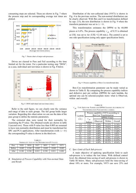
Distribution of the raw-collected data (V073) is shown in
Fig. 4 in the previous section. The non-normal distribution can
be clearly observed. With Box and Cox transformation defined
by eqn. (13), the new distribution is shown in Fig. 9 where the
transform parameter was set to = 0 .
This transformation estimates the DPPM to be 68,000
pieces or 6.8%. The process capability C pk
of 0.53 is obtained
as USL was set to 6σ (USL=12.48 min.). The control is set to
one side specification (using only upper specification limit).
Fig. 7 Pareto chart of major sub-processes
Drives are classed to Pass and Fail according to the time
limited set for the tester. For a particular testing step “D036”,
as a case, individual unit test times is shown in Fig. 8 below.
Fig. 9 Process capability of Box-Cox transformed data
Box-Cox transformation parameter can be made varied as
shown in Table II. By comparing the process capability indices
and defective part per million (DPPM) for each lambda, the
optimal one can be selected.(explain more: what is Observed,
within and overall)
Fig. 8 D036 individual unit test times (min.)
Refer to the said figure, we can clearly note the variance
and range of data in each groups. The fail group holds larger
variation. Regarding this observation we can use the data of the
pass group to define the statistic parameters.
The extracted data were tested for their normality by
examining the P-value. The obtained results are shown in table
I (second row). Those with P-value less than 0.005 are assumed
to have non-normality distribution and must be transformed for
SPC and PCA applications. After transformation (with = 0 )
the corresponding P-value is shown in the third row.
TABLE I
NORMALITY TEST OF THE DISTRIBUTION (P-VALUE)
Proc. V020 D036 V037 S055 V071 V073
Before