An Application of SPC and PCA in a Product Manufacturing: Energy ...
An Application of SPC and PCA in a Product Manufacturing: Energy ...
An Application of SPC and PCA in a Product Manufacturing: Energy ...

Create successful ePaper yourself
Turn your PDF publications into a flip-book with our unique Google optimized e-Paper software.
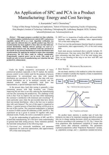
<strong>An</strong> <strong>Application</strong> <strong>of</strong> <strong>SPC</strong> <strong>and</strong> <strong>PCA</strong> <strong>in</strong> a <strong>Product</strong><br />
Manufactur<strong>in</strong>g: <strong>Energy</strong> <strong>and</strong> Cost Sav<strong>in</strong>gs<br />
A. Kaewpukdee #1 <strong>and</strong> S. Choomchuay *2<br />
# College <strong>of</strong> Data Storage Technology <strong>and</strong> <strong>Application</strong>s, * School <strong>of</strong> Electronic Eng<strong>in</strong>eer<strong>in</strong>g, Faculty <strong>of</strong> Eng<strong>in</strong>eer<strong>in</strong>g,<br />
K<strong>in</strong>g Mongkut’s Institute <strong>of</strong> Technology Ladkrabang, Chalongkrung Rd., Ladkrabang, Bangkok 10520, Thail<strong>and</strong>.<br />
1 adisorn44@hotmail.com, 2 kchsomsa@kmitl.ac.th<br />
Abstract— This paper proposes a product test time reduction.<br />
Our method employs statistical process control (<strong>SPC</strong>) <strong>and</strong> process<br />
capability analysis (<strong>PCA</strong>) as a tool. Algorithm verification was<br />
made upon the collected data <strong>of</strong> a specific product type. Box-Cox<br />
transformation has been applied to those data sets that hold nonnormal<br />
distribution. M<strong>in</strong>itab s<strong>of</strong>tware package was used as a<br />
mathematical analysis tool. The obta<strong>in</strong>ed result has conv<strong>in</strong>ced us<br />
the benefit <strong>of</strong> non-normal distribution to normal distribution data<br />
transformation. By apply<strong>in</strong>g the method to major time-consum<strong>in</strong>g<br />
sub-processes, the test times could be reduced considerably.<br />
Proportionally required power can be saved. This study is <strong>of</strong><br />
benefit not only <strong>in</strong> term <strong>of</strong> manufactur<strong>in</strong>g cost reduction but also<br />
productivity enhancement.<br />
2) SRST test; i.e. <strong>in</strong>spection <strong>of</strong> media surface <strong>and</strong> record defect<br />
locations under squeeze condition, takes approximately<br />
76% <strong>of</strong> the total test<strong>in</strong>g time.<br />
3) F<strong>in</strong>al test; test the performance function based on customer<br />
requirements, takes approximately 14% <strong>of</strong> the total test<strong>in</strong>g<br />
time.<br />
Each ma<strong>in</strong> process mentioned above actually <strong>in</strong>cludes 10-<br />
15 sub-processes. One may notice that SRST test is the most<br />
time consum<strong>in</strong>g step that takes 3/4 <strong>of</strong> the total test<strong>in</strong>g time.<br />
Thus, we are focus<strong>in</strong>g at this step to see how well <strong>SPC</strong> <strong>and</strong><br />
<strong>PCA</strong> can help.<br />
I. INTRODUCTION<br />
Under the highly competitive environment <strong>of</strong> many<br />
commercial products especially <strong>in</strong> the IT market, the statistic<br />
process control is now widely used for the purpose <strong>of</strong> process<br />
improvement. In conventional case, data with normal<br />
distribution are considered. For the case that data with nonnormal<br />
distribution are to be analyzed correctly <strong>and</strong> the<br />
obta<strong>in</strong>ed results should consistently hold their true<br />
representation, a special technique must be deployed.<br />
At the present days, hard disk test<strong>in</strong>g is generally a time<br />
consum<strong>in</strong>g process with high <strong>in</strong>ventory cost. Clearly,<br />
improv<strong>in</strong>g the test time is not only reduc<strong>in</strong>g the manufactur<strong>in</strong>g<br />
cost but also <strong>in</strong>creas<strong>in</strong>g the productivity. The challenge <strong>of</strong> the<br />
work is that “Can we improve the test time while ma<strong>in</strong>ta<strong>in</strong><strong>in</strong>g<br />
the customer’s satisfaction with m<strong>in</strong>imum unit rework<strong>in</strong>g” In<br />
some particular cases when the pre-recorded data have shown<br />
their non-normal distribution: -what is the best way to analyze<br />
data with such features The rest <strong>of</strong> this paper is organized as<br />
follows. A general process <strong>of</strong> hard disk test<strong>in</strong>g will be given <strong>in</strong><br />
the rest <strong>of</strong> this section. The concerned mathematics is outl<strong>in</strong>ed<br />
<strong>in</strong> section II whilst section III elaborates <strong>of</strong> <strong>SPC</strong> <strong>and</strong> <strong>PCA</strong>. The<br />
experiment set up is given <strong>in</strong> section IV together with some<br />
obta<strong>in</strong>ed results. F<strong>in</strong>ally, the work is concluded <strong>in</strong> section V.<br />
To get the underst<strong>and</strong><strong>in</strong>g <strong>of</strong> applications <strong>of</strong> <strong>SPC</strong> <strong>and</strong> <strong>PCA</strong><br />
<strong>in</strong> hard disk manufactur<strong>in</strong>g, let’s first have some underst<strong>and</strong><strong>in</strong>g<br />
<strong>of</strong> general hard disk test<strong>in</strong>g process. Some <strong>in</strong>dustries perform<br />
the hard disk test<strong>in</strong>g based on the follow<strong>in</strong>g steps<br />
1) Functional test, microcode <strong>in</strong>stallation, <strong>and</strong> parameter<br />
adjustment for read-write optimization, take approximately<br />
10% <strong>of</strong> the total test<strong>in</strong>g time.<br />
II. MATHEMATIC BACKGROUND<br />
A. Basic Statistics<br />
On one h<strong>and</strong>, statistics is the method to collect the m<strong>in</strong>ority<br />
<strong>of</strong> data or samples to predict the majority <strong>of</strong> data or populations<br />
that one cannot work out all.<br />
Fig. 1 Statistical data analyz<strong>in</strong>g process<br />
<br />
x<br />
Fig. 2 Population <strong>and</strong> Sample<br />
On another h<strong>and</strong>, statistics is another type <strong>of</strong> tools that<br />
<strong>in</strong>terprets raw data to be important mean<strong>in</strong>gs <strong>and</strong> allows people<br />
who are <strong>in</strong> charge mak<strong>in</strong>g decisions which are unnecessary to<br />
be always accord<strong>in</strong>g to the mean<strong>in</strong>gs [1], [2]. Fig. 2 shows the<br />
close population data distributions compared to sample data<br />
under correct data collection conditions. The parameters<br />
expla<strong>in</strong>ed populations called “Population Parameters” <strong>in</strong>clude,<br />
; population average, <strong>and</strong> s ; population st<strong>and</strong>ard deviation.
Parameters expla<strong>in</strong> samples called “Sample Parameters”<br />
<strong>in</strong>clude, x ; sample average, <strong>and</strong> ; sample st<strong>and</strong>ard<br />
deviation.<br />
Available <strong>of</strong> data groups are conventionally used to expla<strong>in</strong><br />
“Sample” or “Populations” to achieve the most po<strong>in</strong>ts <strong>of</strong> view.<br />
One technique that generally applied to expla<strong>in</strong> data is a term<br />
called “central tendency”. There are three basic statistics<br />
parameters available to expla<strong>in</strong> this term; namely mean,<br />
median, <strong>and</strong> mode.<br />
Mean (average or arithmetic mean) is depicted as shown <strong>in</strong><br />
eqn. (1) below. It is widely used <strong>in</strong> most cases.<br />
1<br />
n n<br />
i<br />
x x (1)<br />
i1<br />
Median <strong>and</strong> mode are also applied when data are needed to<br />
be analyzed <strong>in</strong> order to verify that they have natural deviation<br />
because these will affect the central tendency value. Tendency<br />
can be considered as data quality respected to the size <strong>of</strong><br />
deviation or “Dispersion” by measur<strong>in</strong>g various statistics<br />
parameters <strong>in</strong>clude “Range: R ”, “St<strong>and</strong>ard deviation: ” <strong>and</strong><br />
2<br />
“Variance: ” which are given below <strong>in</strong> eqn.(2), (3) <strong>and</strong> (4)<br />
respectively [3].<br />
R x x<br />
(2)<br />
max m<strong>in</strong><br />
po<strong>in</strong>ts l<strong>in</strong>es up around (with<strong>in</strong> an amount <strong>of</strong> discrepancy) the<br />
straight l<strong>in</strong>e <strong>of</strong> normal distribution. P-value > 0.05, implies<br />
normal distribution <strong>of</strong> tested data whilst P-value < 0.05 implies<br />
non-normal distribution <strong>of</strong> tested data.<br />
a) Non-normal distribution b) Normal distribution<br />
Fig. 3 Probability plot <strong>of</strong> non-normal data (P-value
CL x<br />
(7)<br />
LSL<br />
LSL x 3 (8)<br />
Nom<strong>in</strong>al<br />
USL<br />
assumption <strong>of</strong> normality under the specification limits.<br />
Commercial package such as M<strong>in</strong>itab do provide this function<br />
as its st<strong>and</strong>ard. It also <strong>of</strong>fers the calculation <strong>of</strong> the defective<br />
part per million (DPPM) <strong>of</strong> the transformed data. In the<br />
background M<strong>in</strong>itab uses the transformation tool so called<br />
“Box-Cox Transformation”.<br />
Box <strong>and</strong> Cox [4] proposed a family <strong>of</strong> power<br />
transformations on necessarily positive response variable x<br />
given by<br />
<br />
-3σ +3σ<br />
<br />
( x<br />
<br />
1)<br />
( ) i <br />
x , if 0<br />
i<br />
<br />
<br />
<br />
<br />
<br />
ln( xi<br />
), if 0<br />
for 1 i n (13)<br />
Fig. 5 process control st<strong>and</strong>ard at 6σ level<br />
The bound <strong>of</strong> x 3 or 6σ control is widely used as<br />
st<strong>and</strong>ard one. It <strong>of</strong>fers confidence <strong>in</strong>terval <strong>of</strong> 99.73%.<br />
A. Process Capability <strong>An</strong>alysis<br />
Capability <strong>in</strong>dex ( C ) is a parameter <strong>in</strong>dicat<strong>in</strong>g the control<br />
p<br />
range. It implies data deviation <strong>of</strong> populations compared with<br />
the allowed deviation. Mathematical expression <strong>of</strong> the<br />
capability <strong>in</strong>dex is given <strong>in</strong> eqn. (9) below.<br />
USL-LSL<br />
C p <br />
6<br />
Process variation<br />
When samples are considered <strong>in</strong>stead <strong>of</strong> population, x is<br />
used <strong>in</strong>stead <strong>of</strong> . C is now termed as C . Its lower <strong>and</strong><br />
p<br />
upper limits are given with respected to mean x as follows.<br />
pk<br />
(9)<br />
This transformation depends on a s<strong>in</strong>gle parameter that is<br />
estimated us<strong>in</strong>g Maximum likelihood estimation (MLE) [5].<br />
The transformation <strong>of</strong> non-normal data to normal data us<strong>in</strong>g<br />
Box-Cox transformation is available <strong>in</strong> most statistical<br />
s<strong>of</strong>tware packages. Apparently, we can deploy this technique<br />
directly to evaluate <strong>PCA</strong>.<br />
IV. EXPERIMENT<br />
Data from SRST hard disk tester have been studied. 4,000<br />
hard drive units <strong>of</strong> which 2,000 are pass drives <strong>and</strong> the rest are<br />
fail drives. The “pass” <strong>and</strong> “fail” criteria are not classified by<br />
our model. Instead, they are classified by the current<br />
manufactur<strong>in</strong>g criteria that are less related to <strong>SPC</strong> or <strong>PCA</strong>. Fig.<br />
6 shows experiment steps <strong>of</strong> this research. M<strong>in</strong>itab package is<br />
used for data analysis. Upon the analyzed result the control<br />
parameters can be decided. The control model then can be<br />
verified to term out the process capability <strong>and</strong> performance.<br />
USL - x<br />
C pu <br />
3<br />
(10)<br />
C pl<br />
<br />
x - LSL<br />
3<br />
(11)<br />
Fig. 6 Experiment procedure<br />
In practice, the lower one is preferable. Therefore,<br />
C<br />
pk<br />
m<strong>in</strong>( C pu , C<br />
pl<br />
)<br />
(12)<br />
B. Process Capability <strong>An</strong>alysis with Non-normal data<br />
Some to be controlled processes may hold data with nonnormal<br />
feature. When data follows a well-known distribution<br />
type, but non-normal distribution, such as a Weibull or lognormal<br />
distribution, calculation <strong>of</strong> defect rates is accomplished<br />
us<strong>in</strong>g the properties <strong>of</strong> the distribution. Parameters <strong>of</strong> the<br />
distribution <strong>and</strong> the specification limits must be <strong>in</strong>put to the<br />
procedure. Alternatively, those non-normal data can be<br />
mathematically transformed to the approximated normal<br />
distribution <strong>and</strong> calculate the process capability us<strong>in</strong>g the<br />
In this study, we are work<strong>in</strong>g backward. For the process<br />
data we do analysis those data to see whether the process is<br />
stable <strong>and</strong> under control. We use <strong>PCA</strong> to check if we can cut<br />
down the test time. <strong>An</strong>d if <strong>PCA</strong> is applicable –what effect it<br />
produces upon its application; i.e. FAR <strong>and</strong> FRR. Therefore, no<br />
action is taken to the real process. However, this study should<br />
demonstrate the possibility <strong>of</strong> test time improvement.<br />
A. Data Retrieval <strong>and</strong> Extraction<br />
A database file generated by a tester usually conta<strong>in</strong>s<br />
several <strong>in</strong>formation reveal the test<strong>in</strong>g parameters <strong>and</strong> results.<br />
Common to all <strong>and</strong> <strong>of</strong> our <strong>in</strong>terest are test<strong>in</strong>g steps <strong>and</strong><br />
correspond<strong>in</strong>g times spent for such steps. Although the actual<br />
process <strong>in</strong>volves many step sequences, only few time-
consum<strong>in</strong>g steps are selected. These are shown <strong>in</strong> Fig. 7 where<br />
the process step <strong>and</strong> its correspond<strong>in</strong>g average test times are<br />
plotted.<br />
Distribution <strong>of</strong> the raw-collected data (V073) is shown <strong>in</strong><br />
Fig. 4 <strong>in</strong> the previous section. The non-normal distribution can<br />
be clearly observed. With Box <strong>and</strong> Cox transformation def<strong>in</strong>ed<br />
by eqn. (13), the new distribution is shown <strong>in</strong> Fig. 9 where the<br />
transform parameter was set to = 0 .<br />
This transformation estimates the DPPM to be 68,000<br />
pieces or 6.8%. The process capability C pk<br />
<strong>of</strong> 0.53 is obta<strong>in</strong>ed<br />
as USL was set to 6σ (USL=12.48 m<strong>in</strong>.). The control is set to<br />
one side specification (us<strong>in</strong>g only upper specification limit).<br />
Fig. 7 Pareto chart <strong>of</strong> major sub-processes<br />
Drives are classed to Pass <strong>and</strong> Fail accord<strong>in</strong>g to the time<br />
limited set for the tester. For a particular test<strong>in</strong>g step “D036”,<br />
as a case, <strong>in</strong>dividual unit test times is shown <strong>in</strong> Fig. 8 below.<br />
Fig. 9 Process capability <strong>of</strong> Box-Cox transformed data<br />
Box-Cox transformation parameter can be made varied as<br />
shown <strong>in</strong> Table II. By compar<strong>in</strong>g the process capability <strong>in</strong>dices<br />
<strong>and</strong> defective part per million (DPPM) for each lambda, the<br />
optimal one can be selected.(expla<strong>in</strong> more: what is Observed,<br />
with<strong>in</strong> <strong>and</strong> overall)<br />
Fig. 8 D036 <strong>in</strong>dividual unit test times (m<strong>in</strong>.)<br />
Refer to the said figure, we can clearly note the variance<br />
<strong>and</strong> range <strong>of</strong> data <strong>in</strong> each groups. The fail group holds larger<br />
variation. Regard<strong>in</strong>g this observation we can use the data <strong>of</strong> the<br />
pass group to def<strong>in</strong>e the statistic parameters.<br />
The extracted data were tested for their normality by<br />
exam<strong>in</strong><strong>in</strong>g the P-value. The obta<strong>in</strong>ed results are shown <strong>in</strong> table<br />
I (second row). Those with P-value less than 0.005 are assumed<br />
to have non-normality distribution <strong>and</strong> must be transformed for<br />
<strong>SPC</strong> <strong>and</strong> <strong>PCA</strong> applications. After transformation (with = 0 )<br />
the correspond<strong>in</strong>g P-value is shown <strong>in</strong> the third row.<br />
TABLE I<br />
NORMALITY TEST OF THE DISTRIBUTION (P-VALUE)<br />
Proc. V020 D036 V037 S055 V071 V073<br />
Before
D036 can save 14%. However when we look <strong>in</strong>to details, V073<br />
have much less impact. This is because the average test time <strong>of</strong><br />
V073 is only 5.2 m<strong>in</strong>utes whilst that <strong>of</strong> D036 is 435.8 m<strong>in</strong>utes.<br />
Outcomes (yield) <strong>of</strong> each sub-process can be computed based<br />
on the fault rejected drives <strong>and</strong> the total number <strong>of</strong> pass drives.<br />
TABLE III<br />
RESULT AFTER THE APPLICATION OF SPEC. LIMIT TO THE SUB-PROCESS<br />
Proc.<br />
Quality<br />
Level<br />
Spec. limit<br />
m<strong>in</strong>.<br />
C pk<br />
Time<br />
sav<strong>in</strong>g<br />
m<strong>in</strong>.<br />
Time<br />
sav<strong>in</strong>g<br />
%<br />
Yield<br />
%<br />
V020 6 7.65 1.17 19.19 6.73 92.80<br />
D036 3 491.2 1.01 60.00 13.77 99.35<br />
V037 6 4.02 1.20 11.00 7.56 90.80<br />
S055 3 132.48 1.00 14.77 0.21 98.25<br />
V071 6 5.70 1.52 15.72 9.41 95.80<br />
V073 6 12.48 1.30 41.90 24.57 93.20<br />
Apply<strong>in</strong>g only specification limit by mean <strong>of</strong> test times can<br />
result <strong>in</strong> pass drives to be rejected <strong>and</strong> fail drives to be<br />
accepted. In pr<strong>in</strong>ciple, we should reject only the fail drives <strong>and</strong><br />
accept only the pass drives. However, the situation <strong>of</strong> rejection<br />
<strong>of</strong> good drives (termed as fault rejection rate: FRR) <strong>and</strong><br />
acceptance <strong>of</strong> bad drives (termed as fault acceptance rate:<br />
FAR) cannot be totally avoided. We have <strong>in</strong>vestigated the issue<br />
with the merit <strong>of</strong> test times sav<strong>in</strong>g. The result is shown <strong>in</strong> Fig.<br />
10 below. Be kept <strong>in</strong> m<strong>in</strong>d that <strong>in</strong> this experiment all 4,000<br />
units are <strong>in</strong>put to each test<strong>in</strong>g step. If the method proposed <strong>in</strong><br />
this study is brought to practice, the genu<strong>in</strong>e rejected drives<br />
<strong>and</strong> the fault rejected drives will be reworked upon their failure<br />
symptoms. Obviously, the lower FRR is the better. Genu<strong>in</strong>e<br />
pass drives <strong>and</strong> fault accepted drives will be passed to the<br />
subsequent process step. Repeatedly tested for many step<br />
sequences, the fault accepted units should be reduced to<br />
m<strong>in</strong>imum number. In practice, we should not deliver any fail<br />
drives to the customer at all. Ideally, fault accepted drives<br />
should be zero at the f<strong>in</strong>al step.<br />
accepted <strong>and</strong> genu<strong>in</strong>e rejected respectively. As shown <strong>in</strong> Table<br />
III, We fed 4000 product units <strong>in</strong>to the first process step (say<br />
V020). At this step, 1,865 good drives <strong>and</strong> 1,236 bad drives<br />
passed. 144 good drives <strong>and</strong> 764 bad drives were rejected.<br />
Therefore, 3092 drives were fed <strong>in</strong> to the subsequent subprocess<br />
(say D036) where the spec-limit is applied aga<strong>in</strong>. The<br />
similar procedure is applied throughout all sub-process. F<strong>in</strong>ally<br />
only 3 bad drives passed. They are known as good drives (s<strong>in</strong>ce<br />
they were wrongly accepted). From the begg<strong>in</strong>g to the f<strong>in</strong>al<br />
steps, 304 good drives were wrongly rejected (as FR drives).<br />
They must be reworked.<br />
TABLE IV<br />
GRANT AND FAULT ACCEPTANCE BEFORE AND AFTER EACH TEST SEQUENCE<br />
Steps<br />
Proc.<br />
<strong>Product</strong> Unit Count (Pieces)<br />
Input Output GA GR FA FR<br />
1 V020 4,000 3,092 1,865 764 1,236 144<br />
2 D036 3,092 2,393 1,843 686 550 13<br />
3 V037 2,393 2,017 1,797 330 220 46<br />
4 S055 2,017 1,862 1,777 135 85 20<br />
5 V071 1,862 1,793 1,775 67 18 2<br />
6 V073 1,793 1,699 1,696 15 3 79<br />
E. Cost Reduction via Power Sav<strong>in</strong>g<br />
Test<strong>in</strong>g the units, as a matter <strong>of</strong> fact, power is required.<br />
Such cost cannot be avoided. However, sav<strong>in</strong>g the test time is<br />
essentially sav<strong>in</strong>g the electric cost <strong>and</strong> labor cost. The products<br />
under this study do require the power <strong>of</strong> 20 Watt per hour per<br />
product unit (approximately). Power requirement <strong>of</strong> each subprocess<br />
can be computed from:<br />
n<br />
Total power 20Ti<br />
(13)<br />
i1<br />
Where n denote the number <strong>of</strong> unit to be tested <strong>and</strong> T<br />
i<br />
denote the test time <strong>of</strong> the unit i . We have computed power<br />
requirement <strong>in</strong> unit test<strong>in</strong>g before <strong>and</strong> after application <strong>of</strong> <strong>SPC</strong>.<br />
The result is shown <strong>in</strong> table V below. Start with 4000 product<br />
units, without <strong>and</strong> with the application <strong>of</strong> <strong>SPC</strong> we can save the<br />
power up to 140 Kw with the total test time <strong>of</strong> 10.89 hrs.<br />
Fig. 10 Fault rejected drives <strong>and</strong> Fault accepted drives after the application <strong>of</strong><br />
<strong>PCA</strong> to each sub-process<br />
D. Sequential <strong>Application</strong>s <strong>of</strong> Sub-process Spec-Limit<br />
Once we could optimize the specification limit <strong>of</strong> each subprocess,<br />
we can apply the limit to all the process that assumed<br />
to run sequentially. GA <strong>and</strong> GR are st<strong>and</strong><strong>in</strong>g for genu<strong>in</strong>e<br />
Proc.<br />
TABLE V<br />
REQUIRED POWER COMPARISON AND COST SAVINGS<br />
Number<br />
<strong>of</strong> units<br />
Total Power<br />
without <strong>SPC</strong><br />
(Kw)<br />
Total Power<br />
with <strong>SPC</strong><br />
(Kw)<br />
Power<br />
sav<strong>in</strong>g<br />
(Kw)<br />
V020 4,000 31.200 6.400 24.800<br />
D036 3,092 510.180 448.340 61.840<br />
V037 2,393 10.529 1.914 8.614<br />
S055 2,017 89.554 79.873 9.681<br />
V071 1,862 11.544 1.862 9.682<br />
V073 1,793 26.895 1.793 25.102<br />
Total - 679.902 540.182 139.719
F. Actual Time Sav<strong>in</strong>g <strong>and</strong> <strong>Energy</strong> Sav<strong>in</strong>g<br />
The sub-process with low yield can cause several good<br />
drives to be reworked <strong>and</strong> retested. This is the obvious<br />
drawback <strong>of</strong> our method. As a case, for example, the subprocess<br />
D036 holds 436 m<strong>in</strong>utes (average test time) <strong>and</strong> it <strong>of</strong>fer<br />
60 m<strong>in</strong>utes time-sav<strong>in</strong>g after the application <strong>of</strong> <strong>SPC</strong>. However<br />
it rejected 13 drives wrongly. These 13 drives must be<br />
<strong>in</strong>vestigated <strong>and</strong> retested. They could aga<strong>in</strong> take similar test<br />
time <strong>in</strong> their retest<strong>in</strong>g process. Of course, they do consume<br />
energy. The possible energy sav<strong>in</strong>g <strong>of</strong> D036 then decrease.<br />
[4] D. Montgromery, “Introduction <strong>of</strong> statistical quality control”, 5 th<br />
ed., Wiley, New York, 1996.<br />
[5] L. C. Tang, S. E. Than, “Comput<strong>in</strong>g process capability <strong>in</strong>dices for<br />
non-normal data”, 1999.<br />
[6] K. Poypanitchararenpol “Statistics for Eng<strong>in</strong>eer<strong>in</strong>g”, Bangkok,<br />
Technology Promotion Association (TPA) (Thail<strong>and</strong>-Japan),<br />
1999.<br />
[7] T. S<strong>in</strong>charu “Research<strong>in</strong>g <strong>and</strong> <strong>An</strong>alysis Statistics data by SPSS”,<br />
Ed. 9, Bangkok, Bus<strong>in</strong>ess R&D, 2008.<br />
[8] K. Rezaie, B. Ostadi <strong>and</strong> M.R. Taghizadeh. “<strong>Application</strong> <strong>of</strong><br />
Process Capability <strong>and</strong> Process Performance Indices” Journal <strong>of</strong><br />
Applied Sciences 6(5): 1186-1191, 2006.<br />
V. CONCLUSIONS<br />
In this study we have demonstrated the application <strong>of</strong> <strong>SPC</strong><br />
<strong>and</strong> <strong>PCA</strong> to a product manufactur<strong>in</strong>g where hard disk drives<br />
manufactur<strong>in</strong>g was taken as a case. Only sub-processes that<br />
contribute large test times were selected <strong>in</strong> this study. To<br />
overcome the data with nor-normality distribution, Box-Cox<br />
transformation with = 0 was applied. Clearly shown <strong>in</strong> table<br />
III, the test times can be reduced to some certa<strong>in</strong> amount.<br />
About 20% <strong>of</strong> total test time can be saved. The time-sav<strong>in</strong>g can<br />
have a major impact to energy sav<strong>in</strong>g <strong>and</strong> labor cost sav<strong>in</strong>g. In<br />
practice, the control method can be either applied to particular<br />
selected sub-processes or applied to all sub-process. A<br />
drawback <strong>of</strong> the method is that the control still produce fault<br />
accepted units that result<strong>in</strong>g <strong>in</strong> the fail unit to be fed to the<br />
subsequent sub-process. Without other screen<strong>in</strong>g method, the<br />
customer can receive the malfunction unit. This is undesirable.<br />
Moreover, the resulted fault rejected units can pile up the unit<br />
cost because <strong>of</strong> its rework<strong>in</strong>g. When we closely look <strong>in</strong>to the<br />
obta<strong>in</strong>ed yield, the sub-process with lower yield can produce<br />
the large number <strong>of</strong> fault rejected drives. This may concern the<br />
nature <strong>of</strong> data distribution <strong>of</strong> such a sub-process that needs<br />
more <strong>in</strong>vestigation on this characteristic.<br />
ACKNOWLEDGEMENT<br />
This work is supported by “Industry/University<br />
Cooperative <strong>of</strong> Data Storage Technology <strong>and</strong> <strong>Application</strong>s<br />
Research Center (I/UCRC), K<strong>in</strong>g Mongkut’s Institute <strong>of</strong><br />
Technology Ladkrabang <strong>and</strong> National Electronic <strong>and</strong> Computer<br />
Technology Center (NECTEC), National Science <strong>and</strong><br />
Technology Development Agency (NSTDA) under scholarship<br />
HDD-01-51-011M. We would like to thank Hitachi Global<br />
Storage Technologies Company (Thail<strong>and</strong>) for their cont<strong>in</strong>ued<br />
support to this research.<br />
REFERENCES<br />
[1] K. Poypanitchararenpol “Process Capability <strong>An</strong>alysis (<strong>PCA</strong>)”,<br />
Bangkok, Technology Promotion Association (TPA) (Thail<strong>and</strong>-<br />
Japan), 2008.<br />
[2] Ch. Srikeawsew “Statistics Learn<strong>in</strong>g <strong>and</strong> <strong>Application</strong> Website”,<br />
www.statistics.ob.tc<br />
[3] G. E. P. Box <strong>and</strong> D. R. Cox, “<strong>An</strong> analysis <strong>of</strong> transformation”, J.<br />
Roy, Stat Soc. B. 26: 211-252, 1964.