Numerical Simulation of Three-Dimensional Viscous Flows with ...
Numerical Simulation of Three-Dimensional Viscous Flows with ...
Numerical Simulation of Three-Dimensional Viscous Flows with ...

Create successful ePaper yourself
Turn your PDF publications into a flip-book with our unique Google optimized e-Paper software.
1342<br />
ISMAIL-ZADE et al.<br />
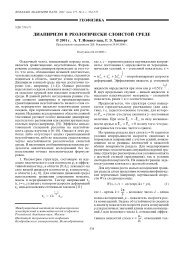
t = 0 t = 60<br />
t = 70<br />
t = 80<br />
t = 100 t = 120<br />
Figure.<br />
The thermally unperturbed density and viscosity have constant values on the characteristics:<br />
ρ *<br />
( t,<br />
x()<br />
t ) = ρ 0 ( xt ( 0 )), µ *<br />
( tx()<br />
t ) = µ 0 ( xt ( 0 )), t ≥ t 0 .<br />
These relations can be used to find density and viscosity in Ω at t > t 0 for the prescribed initial density and<br />
viscosity distributions, provided that the velocity fields at t have already been computed. When trilinear<br />
basis functions are used to approximate density and viscosity, a sufficiently large number <strong>of</strong> independent<br />
modules can be organized to compute the characteristics <strong>of</strong> transport equations and the corresponding densities<br />
and viscosities on them. Note that a finer grid can be used to approximate both density and viscosity,<br />
as compared to the grid used for computing the vector potential.<br />
The temperature T = T(t, x) was approximated by finite-difference methods. The derivatives ∂u i /∂x j were<br />
determined by differentiating the relation u = curly <strong>with</strong> the use <strong>of</strong> (32). Temperature was computed by the<br />
implicit alternating-direction method [26]. At each iteration step in time, a large set <strong>of</strong> linear algebraic systems<br />
<strong>with</strong> tridiagonal matrices was solved, and a corresponding number <strong>of</strong> independent modules could be<br />
organized for parallel solution <strong>of</strong> these systems by means <strong>of</strong> tridiagonal algorithms.<br />
In summary, the numerical solution <strong>of</strong> the problem consisted <strong>of</strong> the following basic stages: (1) a set <strong>of</strong><br />
linear algebraic equations was solved for the coefficients <strong>of</strong> a decomposition <strong>of</strong> the vector velocity potential<br />
in terms <strong>of</strong> basis functions, (2) the heat equation was integrated, and (3) the transport equations for density<br />
and viscosity were integrated. All <strong>of</strong> these stages require substantial computing resources.<br />
7. COMPUTATIONAL PROCEDURES<br />
We briefly describe the procedures to be executed to solve the problem. A uniform discretization <strong>of</strong> the<br />
time axis, t n = t 0 + τn (n ∈ Z), is defined a priori, where τ is the discretization parameter. Next, an iterative<br />
process is organized in which n is consecutively assigned integer values ranging from 0 to m. (The integer<br />
COMPUTATIONAL MATHEMATICS AND MATHEMATICAL PHYSICS Vol. 41 No. 9 2001