A Bradley-Terry Artificial Neural Network Model for Individual ...
A Bradley-Terry Artificial Neural Network Model for Individual ...
A Bradley-Terry Artificial Neural Network Model for Individual ...

You also want an ePaper? Increase the reach of your titles
YUMPU automatically turns print PDFs into web optimized ePapers that Google loves.
Machine Learning manuscript No.<br />
(will be inserted by the editor)<br />
A <strong>Bradley</strong>-<strong>Terry</strong> <strong>Artificial</strong> <strong>Neural</strong> <strong>Network</strong><br />
<strong>Model</strong> <strong>for</strong> <strong>Individual</strong> Ratings in Group<br />
Competitions<br />
Joshua Menke, Tony Martinez<br />
Computer Science Departments, Brigham Young University, 3361 TMCB, Provo,<br />
UT, 84602<br />
Received: date / Revised version: date<br />
Abstract A common statistical model <strong>for</strong> paired comparisons is the <strong>Bradley</strong>-<br />
<strong>Terry</strong> model. The following reparameterizes the <strong>Bradley</strong>-<strong>Terry</strong> model as a<br />
single-layer artificial neural network (ANN) and shows how it can be fitted<br />
using the delta rule. The ANN model is appealing because it gives a flexible<br />
model <strong>for</strong> adding extensions by simply including additional inputs. Several<br />
such extensions are presented that allow the ANN model to learn to predict<br />
the outcome of complex, uneven two-team group competitions by rating<br />
individual players. An active-learning <strong>Bradley</strong>-<strong>Terry</strong> ANN yields a probability<br />
estimate within 5% of the actual value training over 3,379 first-person<br />
shooter matches.
2 Joshua Menke, Tony Martinez<br />
1 Introduction<br />
The <strong>Bradley</strong>-<strong>Terry</strong> model is well known <strong>for</strong> its use in statistics <strong>for</strong> paired<br />
comparisons (<strong>Bradley</strong> & <strong>Terry</strong>, 1952; Davidson & Farquhar, 1976; David,<br />
1988; Hunter, 2004). It has also been applied in machine learning to obtain<br />
multi-class probability estimates (Hastie & Tibshirani, 1998; Zadrozny,<br />
2001; Huang, Lin, & Weng, 2005). The original model says given two subjects<br />
of strengths λ A and λ B , the probability that subject A will defeat or<br />
is better than subject B in a paired-comparison or competition is:<br />
Pr(A def. B) =<br />
λ A<br />
λ A + λ B<br />
. (1)<br />
<strong>Bradley</strong>-<strong>Terry</strong> maximum likelihood models are often fit using methods like<br />
Markov Chain Monte Carlo (MCMC) integration or fixed-point algorithms<br />
that seek the mode of the negative log-likelihood function (Hunter, 2004).<br />
These methods however, “are inadequate <strong>for</strong> large populations of competitors<br />
because the computation becomes intractable.” (Glickman, 1999). The<br />
following paper presents a method <strong>for</strong> determining the ratings of over 4,000<br />
players over 3,379 competitions.<br />
Elo (see, <strong>for</strong> example, (Glickman, 1999)) invented an efficient approach<br />
to iteratively learn the ratings of thousands of players competing in thousands<br />
of chess tournaments. The currently used “ELO Rating System” reparameterizes<br />
the <strong>Bradley</strong>-<strong>Terry</strong> model by setting λ A = e θA yielding:<br />
Pr(A def B) =<br />
1<br />
1 + 10 − θ A −θ B<br />
400<br />
. (2)
An ANN <strong>Model</strong> For <strong>Individual</strong> Ratings in Group Competitions 3<br />
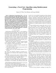
Fig. 1 The <strong>Bradley</strong>-<strong>Terry</strong> Modle as a Single-Layer ANN<br />
The scale specific parameters are historical only and can be changed to the<br />
following:<br />
1<br />
Pr(A def B) = . (3)<br />
1 + e−(θA−θB) Substituting w <strong>for</strong> θ in (3) yields the single-layer artificial neural network<br />
(ANN) in figure 1. This single-layer sigmoid node ANN can be viewed as a<br />
<strong>Bradley</strong>-<strong>Terry</strong> model where the input corresponding to subject A is always<br />
1, and B, always −1. The weights w A and w B correspond to the <strong>Bradley</strong>-<br />
<strong>Terry</strong> strengths θ A and θ B —often referred to as ratings. The <strong>Bradley</strong>-<strong>Terry</strong><br />
ANN model can be fit by using the standard delta rule training method<br />
<strong>for</strong> single-layer ANNs. This ANN interpretation is appealing because many<br />
types of common extensions can be added simply as additional inputs to<br />
the ANN.
4 Joshua Menke, Tony Martinez<br />
The <strong>Bradley</strong>-<strong>Terry</strong> model that Elo’s method will fit can learn the ratings<br />
of subjects competing against other subjects, but does not provide <strong>for</strong> the<br />
case where each subject is a group and the goal is to obtain the ratings of<br />
the individuals in the group. The following presents a model that can give<br />
individual ratings from groups and shows further extensions of the model to<br />
handle “home field advantage”, weighting players by contribution, dealing<br />
with variable sized groups, and other issues. The probability estimates given<br />
by the final model are accurate to within 5% of the actual observed values<br />
over 3,379 competitions in an objective-oriented online first-person shooter.<br />
This article will proceed as follows: section 2 gives more background on<br />
prior uses and methods <strong>for</strong> the fitting of <strong>Bradley</strong>-<strong>Terry</strong> models, section 3<br />
explains the proposed model, extensions, and how to fit it, section 4 explains<br />
how the model is evaluated, section 5 gives results and analysis of<br />
the model’s evaluations, a discussion of possible applications of the model<br />
are given in section 6, and section 7 gives conclusions and future research<br />
directions.<br />
2 Background<br />
The <strong>Bradley</strong>-<strong>Terry</strong> model was originally introduced in (<strong>Bradley</strong> & <strong>Terry</strong>,<br />
1952). It has been widely applied in situations where the strength of a particular<br />
choice or individual needs to be evaluated with respect to another.<br />
This includes sports and other competitive applications. Reviews on the<br />
extensions and methods of fitting <strong>Bradley</strong>-<strong>Terry</strong> models can be found in
An ANN <strong>Model</strong> For <strong>Individual</strong> Ratings in Group Competitions 5<br />
(<strong>Bradley</strong> & <strong>Terry</strong>, 1952; Davidson & Farquhar, 1976; David, 1988; Hunter,<br />
2004). This paper differs from previous research in two ways. First, it proposes<br />
a method to determine individual ratings and rankings when the subjects<br />
being compared are groups. (Huang et al., 2005) proposed a similar<br />
extension, however their method of fitting the model assumes that “each<br />
individual <strong>for</strong>ms a winning or losing team in some competitions which together<br />
involve all subjects” In situations involving thousands of players on<br />
teams that may never compete against each other, their method is not guaranteed<br />
to converge. In addition, they could not prove the method of fitting<br />
would converge to the global minimum. The following method, however, will<br />
always converge to the global minimum because it is an ANN trained with<br />
the delta rule—a method whose convergence properties are well-known. Perhaps<br />
more importantly, the model proposed by (Huang et al., 2005) fits each<br />
parameter simultaneously, which is both impractical when the amount of<br />
competitions and individuals is large, and undesirable if the model needs to<br />
be updated after every competition. This is because new individuals may<br />
enter the model at any point, and there<strong>for</strong>e it is impossible to know when<br />
to stop and fit all the individual parameters. This leads to the second additional<br />
contribution of this paper.<br />
The more common methods <strong>for</strong> fitting a <strong>Bradley</strong>-<strong>Terry</strong> model require<br />
that all of the comparisons to be considered involving all of the competitors<br />
have already taken place so the model can be fit simultaneously. While this<br />
can be more theoretically accurate, it is intractable in situations involving
6 Joshua Menke, Tony Martinez<br />
thousands of comparisions and competitors. In addition, as mentioned, it is<br />
impossible to fit a model this way if new individuals can be added at any<br />
point. Elo and (Glickman, 1999) have both proposed methods <strong>for</strong> approximating<br />
a simultaneous fit by by adapting the <strong>Bradley</strong>-<strong>Terry</strong> model after<br />
every comparison. This also allows <strong>for</strong> new individuals to be inserted at any<br />
point in the model. However, neither of these methods has been extended to<br />
extract individual ratings from groups. The model presented here does allow<br />
individual ratings to be determined in addition to providing an efficient<br />
update after each comparison.<br />
3 The ANN <strong>Model</strong><br />
The section proceeds as follows: it first presents the basic framework <strong>for</strong><br />
viewing the <strong>Bradley</strong>-<strong>Terry</strong> model as a delta-rule trained single layer ANN<br />
in 3.1, then the next section, 3.2 will show how to extend the model to<br />
learn individual ratings within a group, 3.3 extends the model to allow<br />
different weights <strong>for</strong> each individual based on their contribution, 3.4 shows<br />
how the model can be extened to learn “home field” advantages, 3.5 presents<br />
a heuristic to deal with uncertainty in an individual’s rating, and 3.6 gives<br />
another heuristic <strong>for</strong> preventing rating inflation.<br />
3.1 The Basic <strong>Model</strong><br />
The basis <strong>for</strong> the <strong>Bradley</strong>-<strong>Terry</strong> ANN <strong>Model</strong> begins with the ANN shown<br />
in figure 1. Assuming, without loss of generality, that group A is always the
An ANN <strong>Model</strong> For <strong>Individual</strong> Ratings in Group Competitions 7<br />
winner and the question asked is always what is the probability that team<br />
A will win, the input <strong>for</strong> w A will always be 1 and the input <strong>for</strong> w B will<br />
always be −1. The equation <strong>for</strong> the model can be written as:<br />
1<br />
Output = Pr(A def B) =<br />
. (4)<br />
1 + e−(wA−wB) which is the same as (3), except w A and w B are substituted <strong>for</strong> θ A and θ B .<br />
The model is updated applying the delta rule which is written as follows:<br />
∆w i = ηδx i (5)<br />
where η is a learning rate, δ is the error measured with respect to the output,<br />
and x i is the input <strong>for</strong> w i . The error, δ is usually measured as:<br />
δ = Target Output − Actual Output. (6)<br />
For the ANN <strong>Bradley</strong>-<strong>Terry</strong> model, the target output is always 1 given the<br />
assumption that A will defeat B. The actual output is the output of the<br />
single node ANN. There<strong>for</strong>e, the delta rule error can be rewritten as:<br />
δ = 1 − Pr(A def. B) = 1 − Output, (7)<br />
and the weight updates can be written as:<br />
∆w A = η(1 − Output) (8)<br />
∆w B = −η(1 − Output) (9)<br />
Here, x i is implicit as 1 <strong>for</strong> w A and −1 <strong>for</strong> w B , again since A is assumed to<br />
be the winning team. It is well-known that a single-layer ANN trained with<br />
the delta rule will converge to the global minimum as long as the learning
8 Joshua Menke, Tony Martinez<br />
rate is low enough. This is because the delta rule is using gradient descent<br />
on an error surface that is strictly convex. Notice that the <strong>for</strong>mulation of<br />
the delta rule in (5) does not include the derivative of the sigmoid. The<br />
sigmoid’s derivative, namely Ouput(1 − Output), is also the inverse of the<br />
derivative of a different objective function called cross-entropy. There<strong>for</strong>e,<br />
this version of the delta rule is minimizing the cross-entropy instead of the<br />
squared-error. The cross-entropy of a model is also known as the negative<br />
log-likelihood. This is appealing because the resulting fit will produce the<br />
maximum likelihood estimator. Despite not strictly minimizing the squarederror,<br />
this method will still converge to the global minimum because the<br />
direction of the gradient <strong>for</strong> minimizing either function is always the same. In<br />
summary, the standard <strong>Bradley</strong>-<strong>Terry</strong> model can be fit by reparameterizing<br />
it as a single-layer ANN, and then training it with the delta rule.<br />
3.2 Individial Ratings from Groups<br />
In order to extend the ANN model given in 3.1 to learn individual ratings,<br />
the weights <strong>for</strong> each group are obtained by averaging the ratings of the individuals<br />
in each group. Huang et. al (Huang et al., 2005) used the sum of<br />
each group which in the ANN model is analagous to having each individual<br />
have an input of 1 if they are on the winning team, −1 if they are on<br />
the losing team, and 0 if they are absent. This model assumes that when<br />
there are an uneven number of individuals on each team, the effect of one<br />
individual is the same in all situations. Here the average is used instead so
An ANN <strong>Model</strong> For <strong>Individual</strong> Ratings in Group Competitions 9<br />
that the effect of a difference in the number of individuals can be handled<br />
separately. For example, the home field advantage <strong>for</strong>mulation in section<br />
3.4 uses the relative number of individuals per group as an explicit input<br />
into the ANN. Averaging instead of summing the ratings is also analogous<br />
to normalizing the inputs—a common practice in efficiently training ANNs.<br />
Neither method changes the convergence properties because the error surface<br />
is still strictly convex and the weight updates are still in the correct<br />
direction.<br />
As stated, the weights <strong>for</strong> the ANN model in 1 are obtained as follows:<br />
w A =<br />
w B =<br />
∑<br />
i∈A θ i<br />
(10)<br />
N<br />
∑ A<br />
i∈B θ i<br />
(11)<br />
N B<br />
Where i ∈ A means player i belongs to group A and N A is the number of<br />
individuals in group A. Combining individual ratings in this manner means<br />
that the difference in the perfomance between two different players within<br />
a single competition can not be distinguished. However, after two players<br />
have competed within several different teams, their ratings can diverge. The<br />
weight update <strong>for</strong> each player θ i is equal to the update <strong>for</strong> ∆w team given in<br />
(8):<br />
∀i ∈ A,∆θ i = η(1 − Output) (12)<br />
∀i ∈ B,∆θ i = −η(1 − Output) (13)<br />
where A is the winning team and B is the losing team. In this model,<br />
instead of updating w A and w B directly, each individual receives the same
10 Joshua Menke, Tony Martinez<br />
update, there<strong>for</strong>e indirectly changing the average team ratings w i by the<br />
same amount the update in (8) does <strong>for</strong> ∆w A and ∆w B .<br />
3.3 Weighting Player Contribution<br />
Depending on the type of competition, prior knowledge may suggest certain<br />
individuals within a group are more or less important despite their<br />
ratings. As an example, consider a public online multiplayer competition<br />
where players are free to join and leave either team at any time. All else<br />
being equal, players that remain in the competition longer are expected to<br />
contribute more to the outcome than those who leave early, join late, or divide<br />
their time between teams. There<strong>for</strong>e, it would be appropriate to weight<br />
each player’s contribution to w A or w B by the length of time they spent on<br />
team A and team B. In addition, the update to each player’s rating should<br />
also be weighted by the amount of time the player spends on both teams.<br />
There<strong>for</strong>e, w A is rewritten as an average weighted by time played on both<br />
teams:<br />
w A = ∑ i∈A<br />
t i A<br />
θ i ∑<br />
j∈A tj A<br />
. (14)<br />
Here, t i A means the amount of time player i spent on team A. Weighting can<br />
be used <strong>for</strong> more than just the amount of time an individual participates in a<br />
competition. For example, in sports, it may have been previously determined<br />
that a given position is more important than another. The general <strong>for</strong>m <strong>for</strong>
An ANN <strong>Model</strong> For <strong>Individual</strong> Ratings in Group Competitions 11<br />
adding weighting to the model is:<br />
w A = ∑ i∈A<br />
c i<br />
θ i ∑j∈A<br />
cj<br />
. (15)<br />
where c i is the the contribution weight of individual i. This gives an average<br />
that is weighted by each individual’s contribution compared to the rest<br />
of the individuals’ contributions in the group. Again, neither changes the<br />
convexity of the error surface, nor the direction of the gradient, so it will<br />
still converge to the minimum.<br />
3.4 Home Field Advantage<br />
The common way of modeling home field advantage in a <strong>Bradley</strong>-<strong>Terry</strong><br />
model is to add a parameter learned <strong>for</strong> each “field” into the rating of the<br />
appropriate group. In the ANN model of figure 1, this would be analogous<br />
to adding a new connection with a weight of θ f . If the advantage is in favor<br />
of the winning team, the input <strong>for</strong> θ f is 1, if it is <strong>for</strong> the losing team, that<br />
input is −1. This would be one way to model home field advantage in the<br />
current ANN model. However, since the model uses group averages to <strong>for</strong>m<br />
the weights, the home field advantage model can be expanded to include<br />
situations where there is an uneven amount of individuals in each group (N A<br />
!= N B ). Instead of having a single parameter per field, θ fg is the advantage<br />
<strong>for</strong> group g on field f. The input to the ANN model then becomes 1 <strong>for</strong><br />
the winning team (A) and −1 <strong>for</strong> the losing team (B). This is appealing<br />
because θ fg then represents the worth of an average-rated individual from
12 Joshua Menke, Tony Martinez<br />
group g on field f. The following change to the chosen field inputs, f A and<br />
f B , extends this to handle uneven groups:<br />
N A<br />
f A =<br />
N A + N B<br />
(16)<br />
N B<br />
f B =<br />
N A + N B<br />
(17)<br />
There<strong>for</strong>e, the field inputs are the relative size of each group. The full model<br />
including the field inputs then becomes:<br />
Output = Pr(A def B) =<br />
1<br />
1 + e −(wA−wB+θ fAf A−θ fB f B) . (18)<br />
The weight update after each comparison on field f then extends the deltarule<br />
update from (8) to include the new parameters:<br />
∆θ fA = η(1 − Output) (19)<br />
∆θ fB = −η(1 − Output). (20)<br />
3.5 Rating Uncertainty<br />
One of the problems of the given model is that when an individual partipates<br />
<strong>for</strong> the first time, their rating is assumed to be average. This can result<br />
in incorrect predictions when a newer individual’s true rating is actually<br />
significantly higher or lower than average. There<strong>for</strong>e, it would be appropriate<br />
to include the concept of uncertainty or variance in an individuals rating.<br />
Glickman (Glickman, 1999) derived both a likelihood-based method and a<br />
regular-updating method (like Elo’s) <strong>for</strong> modeling this type of uncertainty<br />
in <strong>Bradley</strong>-<strong>Terry</strong> models. However, his methods did not account <strong>for</strong> finding
An ANN <strong>Model</strong> For <strong>Individual</strong> Ratings in Group Competitions 13<br />
individual ratings within groups. Instead of extending his models to do so,<br />
we give the following heuristic which models uncertainty without negatively<br />
impacting the gradient descent method.<br />
Given g i , the number of times that individual i has participated in a<br />
comparision, let the certainty γ i of that individual be:<br />
γ i = min(g i,G)<br />
G<br />
(21)<br />
where G is a constant that represents the number of comparisons needed<br />
be<strong>for</strong>e individual i’s rating is fully trusted. The overall certainty of the comparison<br />
is then the average certainty of the individuals from both groups. If<br />
a weighting is used, then the certainty <strong>for</strong> the comparison is the weighted<br />
average of all the individuals in either group. The probability estimate then<br />
becomes:<br />
Output = Pr(A def B) =<br />
1<br />
1 + e −(C(wA−wB)+θ fAf A−θ fB f B) , (22)<br />
where C is the average certainty of all of the individuals participating in<br />
the comparison. This effectively stretches the logistic function, making the<br />
probability estimate more likely to tend towards 0.5—which is desirable in<br />
more uncertain comparisons. For example, a comparision yielding a 70%<br />
chance of group A defeating group B with C = 1.0 would yield a 60%<br />
chance of group A winning if C = 0.5. The modified weight update appears<br />
as follows:<br />
∀i ∈ A,∆θ i = Cη(1 − Output) (23)<br />
∀i ∈ B,∆θ i = −Cη(1 − Output). (24)
14 Joshua Menke, Tony Martinez<br />
Since this can also be seen to effectively lower the learning rate, η is in<br />
practice chosen to be twice as large <strong>for</strong> the individual updates as the fieldgroup<br />
updates.<br />
The downside to this method of modeling uncertainty is that is does<br />
not allow <strong>for</strong> a later change in an individuals rating due to long periods of<br />
inactivity or due to improving rating over time. This could be implemented<br />
with a <strong>for</strong>m of certainty decay that lowered an individual’s certainty value<br />
γ i , over time. Also, notice a similar measure of uncertainty could be applied<br />
to the field-group parameters.<br />
3.6 Preventing Rating Inflation<br />
One of the problems with averaging (or summing) individual ratings is that<br />
there is no way to model a single individual’s expected contribution based<br />
on their rating. An individual with a rating significantly higher or lower<br />
than a group they participate in will have an equal update to the rest of<br />
the group. This can result in inflating that individual’s rating if they constantly<br />
win with weaker groups. Likewise, a weaker individual participating<br />
in a highly-skilled but losing group may have their rating decreased farther<br />
than is appropriate because that weaker individual was not expected<br />
to help their group win as much as the higher rated individuals were. One<br />
heuristic to offset this problem is to use an individual’s own rating instead<br />
of that individual’s group rating when comparing that individual to the<br />
other group. This will result in individuals with ratings higher than their
An ANN <strong>Model</strong> For <strong>Individual</strong> Ratings in Group Competitions 15<br />
group’s average receiving smaller updates than the rest of the group when<br />
their group wins, and larger negative updates when they lose. The opposite<br />
is true <strong>for</strong> individuals with ratings lower than their group’s average. They<br />
will be larger when they win, and smaller when they lose. This attempts<br />
to account <strong>for</strong> situations where there are large differences in the expected<br />
worth of participating individuals.<br />
4 Methods<br />
The final model employs all of the extensions discussed in section 3. The<br />
model was developed originally to rate players and predict the outcome of<br />
matches in the World War II-based online team first-person shooter computer<br />
game Enemy Territory. With hundreds of thousands of players over<br />
thousands of servers worldwide, Enemy Territory is one of the most popular<br />
multiplayer first-person shooters available. In this game, two teams of<br />
between 4-20 players each, the Axis and the Allies, compete on a given<br />
“map”. Both teams have objectives they need to accomplish on the map to<br />
defeat the other team. Whichever team accomplishes their objectives first<br />
is declared the winner of that map. Usually one of the teams has a timebased<br />
objective—they need to prevent the other team from accomplishing<br />
their objectives <strong>for</strong> a certain period of time. If they do so, they are the<br />
winner. In addition, the objectives <strong>for</strong> one team on a given map can be<br />
easier or harder than the other team’s objectives. The size of either team<br />
can also be different and players can both enter, leave, and change teams
16 Joshua Menke, Tony Martinez<br />
at will during the play of the given map. These are common characteristics<br />
of public Enemy Territory servers and are the reasons the above extensions<br />
were developed. Weighting individuals by time deals with players coming,<br />
going, and changing teams. Incorporating a team size-based “home field advantage”<br />
extension deals with both the uneven numbers and the difference<br />
in difficulty <strong>for</strong> either team on a given map. The certainty parameter was<br />
developed to deal with inflated probability estimates given several new and<br />
not fully tested players. Since it is common practice <strong>for</strong> a server to drop a<br />
player’s rating in<strong>for</strong>mation if they do not play on the server <strong>for</strong> an extended<br />
period of time, no decay in the player’s certainty was deemed necessary.<br />
The model was developed to predict the outcome <strong>for</strong> a given set of teams<br />
playing a macth on a given map. There<strong>for</strong>e, the individual and field-group<br />
parameters (in this case both an Axis and Allies parameter <strong>for</strong> each map)<br />
are updated after the winner is declared <strong>for</strong> each match.<br />
In addition, the model was developed <strong>for</strong> use on public Enemy Territory<br />
servers where a large number of individuals come and go and a single individual<br />
will never eventually see all of the other possible individuals throughout<br />
all of the maps they participate in. In fact, it is common <strong>for</strong> individuals that<br />
play very often to never play together (on either team) because of issues<br />
like time zones. There<strong>for</strong>e, the primary assumption in the method to fit<br />
proposed by (Huang et al., 2005) is not met.<br />
In order to evaluate the effectiveness of the model, its extensions, and<br />
training method, data was collected from 3,379 competitions including 4,249
An ANN <strong>Model</strong> For <strong>Individual</strong> Ratings in Group Competitions 17<br />
players and 24 unique maps. The data included which players participated<br />
in each map, how long they played on each team, which team won the map,<br />
and how long the map lasted. The ANN model is trained as described in<br />
section 3, using the update rule after every map. The model is evaluated<br />
four times, once with no heuristics, once with only the certainty heuristic<br />
from section 3.5, once with only the rating inflation prevention heuristic<br />
from section 3.6, and once combining both heuristics. One way to measure<br />
the effectiveness of these runs would be to look at how often the team with<br />
the higher probability of winning does not actually win. However, this result<br />
can be misleading because it assumes a team with a 55% chance of winning<br />
should win 100% of the time—which is not desirable. The real question is<br />
whether or not a team given a P% chance of winning actually wins P% of<br />
the time. There<strong>for</strong>e, the method of judging the model’s effectiveness chosen<br />
uses a histogram to measure how often a team given a P% chance of winning<br />
actually wins. For the results in section 5, the size of the histogram invertals<br />
is chosen to be 1%. This measure will be called the prediction error because<br />
it shows how far off the predicted outcome is from the actual result. A<br />
prediction error of 5% means that when the model predicts team A has a<br />
70% probability of winning, they may really have a probability of winning<br />
between 65-75%. Or, in the histogram sense, it means that given all of the<br />
occurences of the the model giving a team a 70% chance of winning, that<br />
team may actually win in 65%-75% of those occurences.
18 Joshua Menke, Tony Martinez<br />
Table 1 Bradly-<strong>Terry</strong> ANN Enemy Territory Prediction Errors<br />
Heuristic None Inflation Certainty Both<br />
Prediction Error 0.1034 0.0635 0.0600 0.0542<br />
5 Results and Analysis<br />
The results are shown in table 1. Each column gives the prediction error<br />
resulting from a different combination of heuristics. The first column uses<br />
no heuristics, the second uses only the inflation prevention heuristic (see<br />
section 3.6), the third column uses only the rating certainty heuristic (see<br />
section 3.5), and the final column combines both heuristics. Each heuristic<br />
improves the results and combining both gives the lowest prediction error<br />
at 5.42%. This value means that a given estimate is, on average, 5.42% too<br />
high or 5.42% too low. There<strong>for</strong>e, when the model predicts a team has a<br />
75% chance of winning, the actual % chance of winning may be between 70-<br />
80%. One question is on which side does the prediction error tend <strong>for</strong> a given<br />
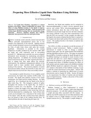
probability. To examine this, the predictions <strong>for</strong> the case that combines both<br />
heuristics are plotted against their prediction errors in figure 2 taking a 5%<br />
interval histogram of the results. The figure shows which direction the error<br />
goes <strong>for</strong> a given prediction. Notice that with only two low-error exceptions on<br />
the extremes, the prediction error tends to be positive when the prediction<br />
probability is low, and negative when it is high. This means the prediction<br />
is slightly extreme on average. For example, if the model predicts a team<br />
is 75% likely to win, they will be on average only 70% likely to win. A
An ANN <strong>Model</strong> For <strong>Individual</strong> Ratings in Group Competitions 19<br />
error<br />
−0.05 0.00 0.05<br />
0.0 0.2 0.4 0.6 0.8 1.0<br />
prediction<br />
Fig. 2 Prediction vs. Prediction Error<br />
team predicted to be 25% likely to win will be on average 30% likely to<br />
win. Since the estimate is extreme, applying a <strong>for</strong>m of empirical Bayes may<br />
be appropriate since it may move the maximum likelihood estimate closer<br />
to the true estimate on average. This would require gathering data from<br />
several servers and finding the prior distribution that generates the mean<br />
ratings of each server. This will be attempted in future work.<br />
In addition to evaluating the model analytically, the ratings it assigns<br />
to the players can be asssessed from experience. Table 2 gives the ratings of<br />
the top ten rated players from the 3,379 games. Several of the players listed<br />
in the top ten are well-known on the server <strong>for</strong> their tenacity in winning<br />
maps, and there<strong>for</strong>e the model’s ranking appears to fit intuition gained from
20 Joshua Menke, Tony Martinez<br />
Table 2 Top Ten Players<br />
Rating θ i<br />
Name<br />
3.64 [TKF]Triple=xXx=<br />
3.27 C-Hu$tle<br />
3.25 SeXy Hulk<br />
3.21 Raker<br />
3.16 [TKF]Loser<br />
3.01 =LK3=Bravo<br />
2.99 qvitex<br />
2.98 K4F*ChocoShake<br />
2.87 K4F*Boas7<br />
2.82 haroldexperience<br />
with these players. In summary, the model effectively predicts<br />
the outcome of a given map with a prediction error of only 5%, and provides<br />
recongizable ratings <strong>for</strong> the players.<br />
6 Application<br />
One of the goals in creating an enjoyable multiplayer game or running an enjoyable<br />
muliplayer game server is keeping the gameplay fair <strong>for</strong> both teams.<br />
Players are more likely to continue playing a game or continue playing on<br />
a given game server if the competiton is neither too easy nor too hard.<br />
When the gameplay is uneven, players tend to become discouraged and<br />
leave server or play different games. Here is where the rating system be-
An ANN <strong>Model</strong> For <strong>Individual</strong> Ratings in Group Competitions 21<br />
comes useful. Besides being able to rate individual players and predict the<br />
outcome of matches in a muliplayer game like Enemy Territory, the predictions<br />
can also be used during a given map to balance the teams. If a team<br />
is more than a chosen threshold P% likely to win, a player can be moved<br />
from that team to the other team in order to “even the odds.” The Bradly-<br />
Territory ANN model as adapted <strong>for</strong> Enemy Territory is now being run on<br />
hundreds of Enemy Territory servers involving hundreds of thousands of<br />
players world-wide. A large number of those servers have enabled an option<br />
that keeps the teams balanced, and there<strong>for</strong>e, in theory, keeps the gameplay<br />
enjoyable <strong>for</strong> the players.<br />
One extension of this system would be to track player ratings across multiple<br />
servers world-wide with a master server and then recommend servers to<br />
players based on the difficulty level of each server. This would allow players<br />
to find matches <strong>for</strong> a given online game in which the gameplay felt “even”<br />
to them. This type of “difficulty matching” is already used in several online<br />
games today, but only <strong>for</strong> either one-on-one type matches, or teams where<br />
the players never change. The given Bradly-<strong>Terry</strong> ANN model could extend<br />
this to allow <strong>for</strong> dynamic teams on public servers that maintain an even<br />
balance of play.<br />
This can also be applied to improving groups chosen <strong>for</strong> sports or military<br />
purposes. <strong>Individual</strong>s can be rated within groups as long as they are<br />
shuffled through several groups and then, over time, groups can be either<br />
chosen by using the highest rated individuals, or balanced by chosing a
22 Joshua Menke, Tony Martinez<br />
mix <strong>for</strong> each group. The higher-rated groups would be appropriate <strong>for</strong> real<br />
encounters, whereas balanced groups may be preferred <strong>for</strong> practicing or<br />
training purposes.<br />
7 Conclusions and Future Work<br />
This paper has presented a method to learn Bradly-<strong>Terry</strong> models using an<br />
ANN. An ANN model is appealing because extensions can be added as new<br />
inputs into the ANN. The basic model is extended to rate individuals where<br />
groups are being compared, to allow <strong>for</strong> weighting individuals, to model<br />
“home field advantages”, to deal with rating uncertainty, and to prevent<br />
rating inflation. The results when applied to a large, real-world problem<br />
including thousands of comparisons involving thousands of players yields<br />
probability prediction estimates within 5% of the actual values. Besides<br />
the a<strong>for</strong>ementioned application of empirical Bayes, two additional areas <strong>for</strong><br />
future work will include 1) extending the model to incorporate temporal<br />
in<strong>for</strong>mation <strong>for</strong> given objectives and 2) attempting to model higher-level<br />
interactions.<br />
In many applications, including sports, military encounters, and online<br />
games like Enemy Territory, there are known objectives that need to be<br />
accomplished in order <strong>for</strong> a given group to defeat another group. In sports,<br />
this may include scoring points, in military encounters, completing subobjectives<br />
<strong>for</strong> a given mission, and in Enemy Territory, each map has a<br />
known list of objectives that both teams need to accomplish to defeat the
An ANN <strong>Model</strong> For <strong>Individual</strong> Ratings in Group Competitions 23<br />
other team. For example, on one map, the Allies must dynamite three known<br />
objectives. A useful piece of in<strong>for</strong>mation is how much time passes be<strong>for</strong>e one<br />
of these objectives is accomplished. If they are accomplished in a faster than<br />
average time, the team may be more likely to win than expected. If a team<br />
takes a longer than average amount of time, their probability of winning may<br />
be lower than expected. In the simplest case, the model can be extended to<br />
take into account not only which team won, but how long it took to win.<br />
One of the next pieces of future research will extend the Bradly-Territory<br />
ANN to incorporate this time-based in<strong>for</strong>mation.<br />
One of the nice properties of using an ANN as a Bradly-<strong>Terry</strong> model<br />
is that it can be easily extended from a single-layer model to a multi-layer<br />
ANN. The convergence guarantees change—namely the model is guaranteed<br />
to converge only to a local minimum, but the representational power<br />
increases. No currently known Bradly-<strong>Terry</strong> model incorporates interaction<br />
effects between teammates and between opponents. Current models do not<br />
consider that player i and player j may have a higher effective rating when<br />
playing together than apart. A multilayer ANN is able to model these interactions,<br />
and there<strong>for</strong>e a future Bradly-<strong>Terry</strong> model will be a multi-layer<br />
Bradly-<strong>Terry</strong> ANN. One of the downsides of using a multi-layer ANN is<br />
that it will be harder to interpret the individual player ratings. There<strong>for</strong>e,<br />
statistical approaches including hierarchical Bayes will also be applied to<br />
see if a more identifiable model can be contructed. One way to develop an<br />
identifiable interaction model can extend from the fact that it is commmon
24 Joshua Menke, Tony Martinez<br />
<strong>for</strong> sub-groups of players to play in “fire-teams” in games like Enemy Territory.<br />
An interaction model can be designed that uses the fire-teams as<br />
a basis without needing to consider the intractable number of all-possible<br />
interactions.<br />
References<br />
<strong>Bradley</strong>, R., & <strong>Terry</strong>, M. (1952). The rank analysis of incomplete block<br />
designs I: The method of paired comparisions. Biometrika, 39, 324–<br />
345.<br />
David, H. A. (1988). The method of paired comparisons. Ox<strong>for</strong>d University<br />
Press.<br />
Davidson, R. R., & Farquhar, P. H. (1976). A bibliography on the method<br />
of paired comparisons. Biometrics, 32, 241–252.<br />
Glickman, M. E. (1999). Parameter Estimation in Large Dynamic Paired<br />
Comparison Experiments. Applied Statistics, 48(3), 377–394.<br />
Hastie, T., & Tibshirani, R. (1998). Classification by pairwise coupling. In<br />
M. I. Jordan, M. J. Kearns, & S. A. Solla (Eds.), Advances in neural<br />
in<strong>for</strong>mation processing systems (Vol. 10). The MIT Press.<br />
Huang, T.-K., Lin, C.-J., & Weng, R. C. (2005). A generalized bradleyterry<br />
model: From group competition to individual skill. In L. K.<br />
Saul, Y. Weiss, & L. Bottou (Eds.), Advances in neural in<strong>for</strong>mation<br />
processing systems 17 (p. 601-608). Cambridge, MA: MIT Press.
An ANN <strong>Model</strong> For <strong>Individual</strong> Ratings in Group Competitions 25<br />
Hunter, D. R. (2004). Mm algorithms <strong>for</strong> generalized <strong>Bradley</strong>-<strong>Terry</strong> models.<br />
The Annals in Statistics, 32, 386–408.<br />
Zadrozny, B. (2001). Reducing multiclass to binary by coupling probability<br />
estimates.