A Probability Course for the Actuaries A Preparation for Exam P/1

A Probability Course for the Actuaries 

A Preparation for Exam P/1 

Marcel B. Finan 

Arkansas Tech University 

c○All Rights Reserved 

Preliminary Draft

2 

In memory of my mother 

August 1, 2008

Contents 

Preface 7 

Risk Management Concepts . . . . . . . . . . . . . . . . . . . . . . 8 

Basic Operations on Sets 11 

1 Basic Definitions . . . . . . . . . . . . . . . . . . . . . . . . . . . 12 

2 Set Operations . . . . . . . . . . . . . . . . . . . . . . . . . . . . 19 

Counting and Combinatorics 33 

3 The Fundamental Principle of Counting . . . . . . . . . . . . . . 33 

4 Permutations and Combinations . . . . . . . . . . . . . . . . . . . 39 

5 Permutations and Combinations with Indistinguishable Objects . 49 

Probability: Definitions and Properties 59 

6 Basic Definitions and Axioms of Probability . . . . . . . . . . . . 59 

7 Properties of Probability . . . . . . . . . . . . . . . . . . . . . . . 67 

8 Probability and Counting Techniques . . . . . . . . . . . . . . . . 75 

Conditional Probability and Independence 81 

9 Conditional Probabilities . . . . . . . . . . . . . . . . . . . . . . . 81 

10 Posterior Probabilities: Bayes’ Formula . . . . . . . . . . . . . . 89 

11 Independent Events . . . . . . . . . . . . . . . . . . . . . . . . . 100 

12 Odds and Conditional Probability . . . . . . . . . . . . . . . . . 109 

Discrete Random Variables 113 

13 Random Variables . . . . . . . . . . . . . . . . . . . . . . . . . . 113 

14 Probability Mass Function and Cumulative Distribution Function118 

15 Expected Value of a Discrete Random Variable . . . . . . . . . . 126 

16 Expected Value of a Function of a Discrete Random Variable . . 133 

3

4 CONTENTS 

17 Variance and Standard Deviation . . . . . . . . . . . . . . . . . 140 

18 Binomial and Multinomial Random Variables . . . . . . . . . . . 146 

19 Poisson Random Variable . . . . . . . . . . . . . . . . . . . . . . 160 

20 Other Discrete Random Variables . . . . . . . . . . . . . . . . . 170 

20.1 Geometric Random Variable . . . . . . . . . . . . . . . . 170 

20.2 Negative Binomial Random Variable . . . . . . . . . . . . 177 

20.3 Hypergeometric Random Variable . . . . . . . . . . . . . 184 

21 Properties of the Cumulative Distribution Function . . . . . . . 190 

Continuous Random Variables 205 

22 Distribution Functions . . . . . . . . . . . . . . . . . . . . . . . 205 

23 Expectation, Variance and Standard Deviation . . . . . . . . . . 217 

24 The Uniform Distribution Function . . . . . . . . . . . . . . . . 235 

25 Normal Random Variables . . . . . . . . . . . . . . . . . . . . . 240 

26 Exponential Random Variables . . . . . . . . . . . . . . . . . . . 255 

27 Gamma and Beta Distributions . . . . . . . . . . . . . . . . . . 265 

28 The Distribution of a Function of a Random Variable . . . . . . 277 

Joint Distributions 285 

29 Jointly Distributed Random Variables . . . . . . . . . . . . . . . 285 

30 Independent Random Variables . . . . . . . . . . . . . . . . . . 299 

31 Sum of Two Independent Random Variables . . . . . . . . . . . 310 

31.1 Discrete Case . . . . . . . . . . . . . . . . . . . . . . . . 310 

31.2 Continuous Case . . . . . . . . . . . . . . . . . . . . . . . 315 

32 Conditional Distributions: Discrete Case . . . . . . . . . . . . . 324 

33 Conditional Distributions: Continuous Case . . . . . . . . . . . . 331 

34 Joint Probability Distributions of Functions of Random Variables 340 

Properties of Expectation 347 

35 Expected Value of a Function of Two Random Variables . . . . . 347 

36 Covariance, Variance of Sums, and Correlations . . . . . . . . . 357 

37 Conditional Expectation . . . . . . . . . . . . . . . . . . . . . . 370 

38 Moment Generating Functions . . . . . . . . . . . . . . . . . . . 381 

Limit Theorems 397 

39 The Law of Large Numbers . . . . . . . . . . . . . . . . . . . . . 397 

39.1 The Weak Law of Large Numbers . . . . . . . . . . . . . 397 

39.2 The Strong Law of Large Numbers . . . . . . . . . . . . . 403

CONTENTS 5 

40 The Central Limit Theorem . . . . . . . . . . . . . . . . . . . . 414 

41 More Useful Probabilistic Inequalities . . . . . . . . . . . . . . . 424 

Appendix 431 

42 Improper Integrals . . . . . . . . . . . . . . . . . . . . . . . . . . 431 

43 Double Integrals . . . . . . . . . . . . . . . . . . . . . . . . . . . 438 

44 Double Integrals in Polar Coordinates . . . . . . . . . . . . . . . 451 

BIBLIOGRAPHY 456

6 CONTENTS

Preface 

The present manuscript is designed mainly to help students prepare for the 

Probability Exam (Exam P/1), the first actuarial examination administered 

by the Society of Actuaries. This examination tests a student’s knowledge of 

the fundamental probability tools for quantitatively assessing risk. A thorough 

command of calculus is assumed. 

More information about the exam can be found on the webpage of the Society 

of Actauries www.soa.org. 

Problems taken from samples of the Exam P/1 provided by the Casual Society 

of Actuaries will be indicated by the symbol ‡. 

This manuscript is also suitable for a one semester course in an undergraduate 

course in probability theory. Answer keys to text problems can be found 

by accessing: http://progressofliberty.today.com/finan-1-answers/. 

A complete solution manual is available to instructors using the book. Email: 

mfinan@atu.edu 

This project has been partially supported by a research grant from Arkansas 

Tech University. 

Marcel B. Finan 

Russellville, Ar 

May 2007 

7

8 PREFACE 

Risk Management Concepts 

When someone is subject to the risk of incurring a financial loss, the loss is 

generally modeled using a random variable or some combination of random 

variables. The loss is often related to a particular time interval-for example, 

an individual may own property that might suffer some damage during the 

following year. Someone who is at risk of a financial loss may choose some 

form of insurance protection to reduce the impact of the loss. An insurance 

policy is a contract between the party that is at risk (the policyholder) 

and an insurer. This contract generally calls for the policyholder to pay 

the insurer some specified amount, the insurance premium, and in return, 

the insurer will reimburse certain claims to the policyholder. A claim is all 

or part of the loss that occurs, depending on the nature of the insurance 

contract. 

There are a few ways of modeling a random loss/claim for a particular insurance 

policy, depending on the nature of the loss. Unless indicated otherwise, 

we will assume the amount paid to the policyholder as a claim is the amount 

of the loss that occurs. Once the random variable X representing the loss has 

been determined, the expected value of the loss, E(X) is referred to as the 

pure premium for the policy. E(X) is also the expected claim on the insurer. 

Note that in general, X might be 0 - it is possible that no loss occurs. For a 

random variable X a measure of the risk is the variation of X, σ 2 = Var(X) 

to be introduced in Section 17. The unitized risk or the coefficient of 

variation for the random variable X is defined to be 

√ 

Var(X) 

E(X) 

Partial insurance coverage: It is possible to construct an insurance policy 

in which the claim paid by the insurer is part, but not necessarily all, 

of the loss that occurs. There are a few standard types of partial insurance 

coverage on a basic ground up loss random variable X. 

(i) Excess-of-loss insurance: An excess-of-loss insurance specifies a deductible 

amount, say d. If a loss of amount X occurs, the insurer pays 

nothing if the loss is less than d, and pays the policyholder the amount of 

the loss in excess of d if the loss is greater than d.

RISK MANAGEMENT CONCEPTS 9 

Two variations on the notion of deductible are 

(a) the franchise deductible: a franchise deductible of amount d refers to 

the situation in which the insurer pays 0 if the loss is below d but pays the 

full amount of loss if the loss is above d; 

(b) the disappearing deductible: a disappearing deductible with lower 

limit d and upper limit d ′ (where d < d ′ ) refers to the situation in which the 

insurer pays 0 if the loss is below d, the insurer pays the full loss if the loss 

amount is above d ′ , and the deductible amount reduces linearly from d to 0 

as the loss increases from d to d ′ ; 

(ii) Policy limit: A policy limit of amount u indicates that the insurer 

will pay a maximum amount of u on a claim. 

A variation on the notion of policy limit is the insurance cap. An insurance 

cap specifies a maximum claim amount, say m, that would be paid 

if a loss occurs on the policy, so that the insurer pays the claim up to a 

maximum amount of m. If there is no deductible, this is the same as a policy 

limit, but if there is a deductible of d, then the maximum amount paid by 

the insurer is m = u − d. In this case, the policy limit of amount u is the 

same as an insurance cap of amount u − d 

(iii) Proportional insurance: Proportional insurance specifies a fraction 

α(0 < α < 1), and if a loss of amount X occurs, the insurer pays the policyholder 

αX the specified fraction of the full loss. 

Reinsurance: In order to limit the exposure to catastrophic claims that 

can occur, insurers often set up reinsurance arrangements with other insurers. 

The basic forms of reinsurance are very similar algebraically to the 

partial insurances on individual policies described above, but they apply 

to the insurer’s aggregate claim random variable S. The claims paid 

by the ceding insurer (the insurer who purchases the reinsurance) are referred 

to as retained claims. 

(i) Stop-loss reinsurance: A stop-loss reinsurance specifies a deductible 

amount d. If the aggregate claim S is less than d then the reinsurer pays 

nothing, but if the aggregate claim is greater than d then the reinsurer pays 

the aggregate claim in excess of d.

10 PREFACE 

(ii) Reinsurance cap: A reinsurance cap specifies a maximum amount paid 

by the reinsurer, say m. 

(iii) Proportional reinsurance: Proportional reinsurance specifies a fraction 

α(0 < α < 1), and if aggregate claims of amount S occur, the reinsurer 

pays αS and the ceding insurer pays (1 − α)S.

Basic Operations on Sets 

The axiomatic approach to probability is developed using the foundation of 

set theory, and a quick review of the theory is in order. If you are familiar 

with set builder notation, Venn diagrams, and the basic operations on sets, 

(unions/or, intersections/and and complements/not), then you have a good 

start on what we will need right away from set theory. 

Set is the most basic term in mathematics. Some synonyms of a set are 

class or collection. In this chapter we introduce the concept of a set and its 

various operations and then study the properties of these operations. 

Throughout this book, we assume that the reader is familiar with the following 

number systems: 

• The set of all positive integers 

• The set of all integers 

• The set of all rational numbers 

N = {1, 2, 3, · · · }. 

Z = {· · · , −3, −2, −1, 0, 1, 2, 3, · · · }. 

Q = { a b 

: a, b ∈ Z with b ≠ 0}. 

• The set R of all real numbers. 

• The set of all complex numbers 

where i = √ −1. 

C = {a + bi : a, b ∈ R} 

11

12 BASIC OPERATIONS ON SETS 

1 Basic Definitions 

We define a set A as a collection of well-defined objects (called elements or 

members of A) such that for any given object x either one (but not both) 

of the following holds: 

• x belongs to A and we write x ∈ A. 

• x does not belong to A, and in this case we write x ∉ A. 

Example 1.1 

Which of the following is a well-defined set. 

(a) The collection of good books. 

(b) The collection of left-handed individuals in Russellville. 

Solution. 

(a) The collection of good books is not a well-defined set since the answer to 

the question “Is My Life a good book” may be subject to dispute. 

(b) This collection is a well-defined set since a person is either left-handed or 

right-handed. Of course, we are ignoring those few who can use both hands 

There are two different ways to represent a set. The first one is to list, 

without repetition, the elements of the set. For example, if A is the solution 

set to the equation x 2 − 4 = 0 then A = {−2, 2}. The other way to represent 

a set is to describe a property that characterizes the elements of the set. This 

is known as the set-builder representation of a set. For example, the set A 

above can be written as A = {x|x is an integer satisfying x 2 − 4 = 0}. 

We define the empty set, denoted by ∅, to be the set with no elements. A 

set which is not empty is called a nonempty set. 


List the elements of the following sets. 

(a) {x|x is a real number such that x 2 = 1}. 

(b) {x|x is an integer such that x 2 − 3 = 0}. 

Solution. 

(a) {−1, 1}. 

(b) Since the only solutions to the given equation are − √ 3 and √ 3 and both 

are not integers then the set in question is the empty set

1 BASIC DEFINITIONS 13 


Use a property to give a description of each of the following sets. 

(a) {a, e, i, o, u}. 

(b) {1, 3, 5, 7, 9}. 

Solution. 

(a) {x|x is a vowel}. 

(b) {n ∈ N|n is odd and less than 10} 

The first arithmetic operation involving sets that we consider is the equality 

of two sets. Two sets A and B are said to be equal if and only if they contain 

the same elements. We write A = B. For non-equal sets we write A ≠ B. In 

this case, the two sets do not contain the same elements. 


Determine whether each of the following pairs of sets are equal. 

(a) {1, 3, 5} and {5, 3, 1}. 

(b) {{1}} and {1, {1}}. 

Solution. 

(a) Since the order of listing elements in a set is irrelevant, {1, 3, 5} = 

{5, 3, 1}. 

(b) Since one of the set has exactly one member and the other has two, 

{{1}} ≠ {1, {1}} 

In set theory, the number of elements in a set has a special name. It is 

called the cardinality of the set. We write n(A) to denote the cardinality of 

the set A. If A has a finite cardinality we say that A is a finite set. Otherwise, 

it is called infinite. For infinite set, we write n(A) = ∞. For example, 

n(N) = ∞. 

Can two infinite sets have the same cardinality The answer is yes. If A and 

B are two sets (finite or infinite) and there is a bijection from A to B then 

the two sets are said to have the same cardinality, i.e. n(A) = n(B). 


What is the cardinality of each of the following sets 

(a) ∅. 

(b) {∅}. 

(c) {a, {a}, {a, {a}}}.


Solution. 

(a) n(∅) = 0. 

(b) This is a set consisting of one element ∅. Thus, n({∅}) = 1. 

(c) n({a, {a}, {a, {a}}}) = 3 

Now, one compares numbers using inequalities. The corresponding notion 

for sets is the concept of a subset: Let A and B be two sets. We say that 

A is a subset of B, denoted by A ⊆ B, if and only if every element of A is 

also an element of B. If there exists an element of A which is not in B then 

we write A ⊈ B. 

For any set A we have ∅ ⊆ A ⊆ A. That is, every set has at least two subsets. 

Also, keep in mind that the empty set is a subset of any set. 


Suppose that A = {2, 4, 6}, B = {2, 6}, and C = {4, 6}. Determine which of 

these sets are subsets of which other of these sets. 

Solution. 

B ⊆ A and C ⊆ A 

If sets A and B are represented as regions in the plane, relationships between 

A and B can be represented by pictures, called Venn diagrams. 


Represent A ⊆ B ⊆ C using Venn diagram. 

Solution. 

The Venn diagram is given in Figure 1.1 

Figure 1.1


Let A and B be two sets. We say that A is a proper subset of B, denoted 

by A ⊂ B, if A ⊆ B and A ≠ B. Thus, to show that A is a proper subset of 

B we must show that every element of A is an element of B and there is an 

element of B which is not in A. 


Order the sets of numbers: Z, R, Q, N using ⊂ 

Solution. 

N ⊂ Z ⊂ Q ⊂ R 


Determine whether each of the following statements is true or false. 

(a) x ∈ {x} (b) {x} ⊆ {x} (c) {x} ∈ {x} 

(d) {x} ∈ {{x}} (e) ∅ ⊆ {x} (f) ∅ ∈ {x} 

Solution. 

(a) True (b) True (c) False since {x} is a set consisting of a single element x 

and so {x} is not a member of this set (d) True (e) True (f) False since {x} 

does not have ∅ as a listed member 

Now, the collection of all subsets of a set A is of importance. We denote 

this set by P(A) and we call it the power set of A. 


Find the power set of A = {a, b, c}. 

Solution. 

P(A) = {∅, {a}, {b}, {c}, {a, b}, {a, c}, {b, c}, {a, b, c}} 

We conclude this section, by introducing the concept of mathematical induction: 

We want to prove that some statement P (n) is true for any nonnegative 

integer n ≥ n 0 . The steps of mathematical induction are as follows: 

(i) (Basis of induction) Show that P (n 0 ) is true. 

(ii) (Induction hypothesis) Assume P (1), P (2), · · · , P (n) are true. 

(iii) (Induction step) Show that P (n + 1) is true.



(a) Use induction to show that if n(A) = n then n(P(A)) = 2 n . 

(b) If P(A) has 256 elements, how many elements are there in A 

Solution. 

(a) We apply induction to prove the claim. If n = 0 then A = ∅ and in this 

case P(A) = {∅}. Thus n(P(A)) = 1 = 2 0 . As induction hypothesis, suppose 

that if n(A) = n then n(P(A)) = 2 n . Let B = {a 1 , a 2 , · · · , a n , a n+1 }. Then 

P(B) consists of all subsets of {a 1 , a 2 , · · · , a n } together with all subsets of 

{a 1 , a 2 , · · · , a n } with the element a n+1 added to them. Hence, n(P(B)) = 

2 n + 2 n = 2 · 2 n = 2 n+1 . 

(b) Since n(P(A)) = 256 = 2 8 then n(A) = 8 


Use induction to show ∑ n 

i=1 (2i − 1) = n2 , n ≥ 1. 

Solution. 

If n = 1 we have 1 2 = 2(1)−1 = ∑ 1 

i=1 

(2i−1). Suppose that the result is true 

for up to n. We will show that it is true for n + 1. Indeed, ∑ n+1 

∑ i=1 

(2i − 1) = 

n 

i=1 (2i − 1) + 2(n + 1) − 1 = n2 + 2n + 2 − 1 = (n + 1) 2


Problems 

Problem 1.1 

Consider the experiment of rolling a die. List the elements of the set A={x:x 

shows a face with prime number}. Recall that a prime number is a number 

with only two divisors: 1 and the number itself. 

Problem 1.2 

Consider the random experiment of tossing a coin three times. 

(a) Let S be the collection of all outcomes of this experiment. List the elements 

of S. Use H for head and T for tail. 

(b) Let E be the subset of S with more than one tail. List the elements of 

E. 

(c) Suppose F = {T HH, HT H, HHT, HHH}. Write F in set-builder notation. 

Problem 1.3 

Consider the experiment of tossing a coin three times. Let E be the collection 

of outcomes with at least one head and F the collection of outcomes of more 

than one head. Compare the two sets E and F. 

Problem 1.4 

A hand of 5 cards is dealt from a deck. Let E be the event that the hand 

contains 5 aces. List the elements of E. 

Problem 1.5 

Prove the following properties: 

(a) Reflexive Property: A ⊆ A. 

(b) Antisymmetric Property: If A ⊆ B abd B ⊆ A then A = B. 

(c) Transitive Property: If A ⊆ B and B ⊆ C then A ⊆ C. 

Problem 1.6 

Prove by using mathematical induction that 

1 + 2 + 3 + · · · + n = 

Problem 1.7 

Prove by using mathematical induction that 

1 2 + 2 2 + 3 2 + · · · + n 2 = 

n(n + 1) 

, n ≥ 1. 

2 

n(n + 1)(2n + 1) 

, n ≥ 1. 

6


Problem 1.8 

Use induction to show that (1 + x) n ≥ 1 + nx for all n ≥ 1, where x > −1. 

Problem 1.9 

A caterer prepared 60 beef tacos for a birthday party. Among these tacos, 

he made 45 with tomatoes, 30 with both tomatoes and onions, and 5 with 

neither tomatoes nor onions. Using a Venn diagram, how many tacos did he 

make with 

(a) tomatoes or onions 

(b) onions 

(c) onions but not tomatoes 

Problem 1.10 

A dormitory of college freshmen has 110 students. Among these students, 

75 are taking English, 

52 are taking history, 

50 are taking math, 

33 are taking English and history, 

30 are taking English and math, 

22 are taking history and math, 

13 are taking English, history, and math. 

How many students are taking 

(a) English and history, but not math, 

(b) neither English, history, nor math, 

(c) math, but neither English nor history, 

(d) English, but not history, 

(e) only one of the three subjects, 

(f) exactly two of the three subjects. 

Problem 1.11 

An experiment consists of the following two stages: (1) first a fair die is 

rolled (2) if the number appearing is even, then a fair coin is tossed; if the 

number appearing is odd, then the die is tossed again. An outcome of this 

experiment is a pair of the form (outcome from stage 1, outcome from stage 

2). Let S be the collection of all outcomes. List the elements of S and then 

find the cardinality of S.

2 SET OPERATIONS 19 

2 Set Operations 

In this section we introduce various operations on sets and study the properties 

of these operations. 

Complements 

If U is a given set whose subsets are under consideration, then we call U a 

universal set. Let U be a universal set and A, B be two subsets of U. The 

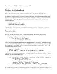
absolute complement of A (See Figure 2.1(I)) is the set 

A c = {x ∈ U|x ∉ A}. 


Find the complement of A = {1, 2, 3} if U = {1, 2, 3, 4, 5, 6}. 

Solution. 

From the definition, A c = {4, 5, 6} 

The relative complement of A with respect to B (See Figure 2.1(II)) is 

the set 

B − A = {x ∈ U|x ∈ B and x ∉ A}. 

Figure 2.1 


Let A = {1, 2, 3} and B = {{1, 2}, 3}. Find A − B. 

Solution. 

The elements of A that are not in B are 1 and 2. That is, A − B = {1, 2} 

Union and Intersection 

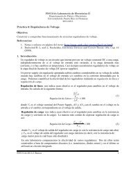
Given two sets A and B. The union of A and B is the set 

A ∪ B = {x|x ∈ A or x ∈ B}


where the ’or’ is inclusive.(See Figure 2.2(a)) 

Figure 2.2 

The above definition can be extended to more than two sets. More precisely, 

if A 1 , A 2 , · · · , are sets then 

∪ ∞ n=1A n = {x|x ∈ A i for some i ∈ N}. 

The intersection of A and B is the set (See Figure 2.2(b)) 

A ∩ B = {x|x ∈ A and x ∈ B}. 


Express each of the following events in terms of the events A, B, and C as 

well as the operations of complementation, union and intersection: 

(a) at least one of the events A, B, C occurs; 

(b) at most one of the events A, B, C occurs; 

(c) none of the events A, B, C occurs; 

(d) all three events A, B, C occur; 

(e) exactly one of the events A, B, C occurs; 

(f) events A and B occur, but not C; 

(g) either event A occurs or, if not, then B also does not occur. 

In each case draw the corresponding Venn diagram. 

Solution. 

(a) A ∪ B ∪ C 

(b) (A ∩ B c ∩ C c ) ∪ (A c ∩ B ∩ C c ) ∪ (A c ∩ B c ∩ C) ∪ (A c ∩ B c ∩ C c ) 

(c) (A ∪ B ∪ C) c = A c ∩ B c ∩ C c 

(d) A ∩ B ∩ C 

(e) (A ∩ B c ∩ C c ) ∪ (A c ∩ B ∩ C c ) ∪ (A c ∩ B c ∩ C) 

(f) A ∩ B ∩ C c


(g) A ∪ (A c ∩ B c ) 


Translate the following set-theoretic notation into event languange. For example, 

“A ∪ B” means “A or B occurs”. 

(a) A ∩ B 

(b) A − B 

(c) A ∪ B − A ∩ B 

(d) A − (B ∪ C) 

(e) A ⊂ B 

(f) A ∩ B = ∅ 

Solution. 

(a) A and B occur 

(b) A occurs and B does not occur 

(c) A or B, but not both, occur 

(d) A occurs, and B and C do not occur 

(e) if A occurs, then B occurs 

(f) if A occurs, then B does not occur 


Find a simpler expression of [(A ∪ B) ∩ (A ∪ C) ∩ (B c ∩ C c )] assuming all 

three sets intersect.


Solution. 

Using a Venn diagram one can easily see that [(A∪B)∩(A∪C)∩(B c ∩C c )] = 

A − [A ∩ (B ∪ C)] 

If A ∩ B = ∅ we say that A and B are disjoint sets. 


Let A and B be two non-empty sets. Write A as the union of two disjoint 

sets. 

Solution. 

Using a Venn diagram one can easily see that A ∩ B and A ∩ B c are disjoint 

sets such that A = (A ∩ B) ∪ (A ∩ B c ) 


Each team in a basketball league plays 20 games in one tournament. Event 

A is the event that Team 1 wins 15 or more games in the tournament. Event 

B is the event that Team 1 wins less than 10 games. Event C is the event 

that Team 1 wins between 8 to 16 games. Of course, Team 1 can win at most 

20 games. Using words, what do the following events represent 

(a) A ∪ B and A ∩ B. 

(b) A ∪ C and A ∩ C. 

(c) B ∪ C and B ∩ C. 

(d) A c , B c , and C c . 

Solution. 

(a) A ∪ B is the event that Team 1 wins 15 or more games or wins 9 or less 

games. A ∩ B is the empty set, since Team 1 cannot win 15 or more games 

and have less than 10 wins at the same time. Therefore, event A and event 

B are disjoint. 

(b) A ∪ C is the event that Team 1 wins at least 8 games. A ∩ C is the event 

that Team 1 wins 15 or 16 games. 

(c) B ∪ C is the event that Team 1 wins at most 16 games. B ∩ C is the 

event that Team 1 wins 8 or 9 games. 

(d) A c is the event that Team 1 wins 14 or fewer games. B c is the event that 

Team 1 wins 10 or more games. C c is the event that Team 1 wins fewer than 

8 or more than 16 games


Given the sets A 1 , A 2 , · · · , we define 

∩ ∞ n=1A n = {x|x ∈ A i for all i ∈ N}. 


For each positive integer n we define A n = {n}. Find ∩ ∞ n=1A n . 

Solution. 

Clealry, ∩ ∞ n=1A n = ∅ 

Remark 2.1 

Note that the Venn diagrams of A ∩ B and A ∪ B show that A ∩ B = B ∩ A 

and A ∪ B = B ∪ A. That is, ∪ and ∩ are commutative laws. 

The following theorem establishes the distributive laws of sets. 

Theorem 2.1 

If A, B, and C are subsets of U then 

(a) A ∩ (B ∪ C) = (A ∩ B) ∪ (A ∩ C). 

(b) A ∪ (B ∩ C) = (A ∪ B) ∩ (A ∪ C). 

Proof. 

See Problem 2.16 

Remark 2.2 

Note that since ∩ and ∪ are commutative operations then (A ∩ B) ∪ C = 

(A ∪ C) ∩ (B ∪ C) and (A ∪ B) ∩ C = (A ∩ C) ∪ (B ∩ C). 

The following theorem presents the relationships between (A ∪ B) c , (A ∩ 

B) c , A c and B c . 

Theorem 2.2 (De Morgan’s Laws) 

Let A and B be subsets of U then 

(a) (A ∪ B) c = A c ∩ B c . 

(b) (A ∩ B) c = A c ∪ B c .


Proof. 

We prove part (a) leaving part(b) as an exercise for the reader. 

(a) Let x ∈ (A ∪ B) c . Then x ∈ U and x ∉ A ∪ B. Hence, x ∈ U and (x ∉ A 

and x ∉ B). This implies that (x ∈ U and x ∉ A) and (x ∈ U and x ∉ B). 

It follows that x ∈ A c ∩ B c . 

Conversely, let x ∈ A c ∩ B c . Then x ∈ A c and x ∈ B c . Hence, x ∉ A and 

x ∉ B which implies that x ∉ (A ∪ B). Hence, x ∈ (A ∪ B) c 

Remark 2.3 

De Morgan’s laws are valid for any countable number of sets. That is 

and 

(∪ ∞ n=1A n ) c = ∩ ∞ n=1A c n 

(∩ ∞ n=1A n ) c = ∪ ∞ n=1A c n 


Let U be the set of people solicited for a contribution to a charity. All the 

people in U were given a chance to watch a video and to read a booklet. Let 

V be the set of people who watched the video, B the set of people who read 

the booklet, C the set of people who made a contribution. 

(a) Describe with set notation: “The set of people who did not see the video 

or read the booklet but who still made a contribution” 

(b) Rewrite your answer using De Morgan’s law and and then restate the 

above. 

Solution. 

(a) (V ∪ B) c ∩ C. 

(b) (V ∪ B) c ∩ C = V c ∩ B c ∩ C = the set of people who did not watch the 

video, did not read the booklet, but did make a contribution 

If A i ∩ A j = ∅ for all i ≠ j then we say that the sets in the collection 

{A n } ∞ n=1 are pairwise disjoint. 


Find three sets A, B, and C that are not pairwise disjoint but A∩B ∩C = ∅. 

Solution. 

One example is A = B = {1} and C = ∅



Find sets A 1 , A 2 , · · · that are pairwise disjoint and ∩ ∞ n=1A n = ∅. 

Solution. 

For each positive integer n, let A n = {n} 


Throw a pair of fair dice. Let A be the event the total is 3, B the event the 

total is even, and C the event the total is a multiple of 7. Show that A, B, C 

are pairwise disjoint. 

Solution. 

We have 

A ={(1, 2), (2, 1)} 

B ={(1, 1), (1, 3), (1, 5), (2, 2), (2, 4), (2, 6)(3, 1), (3, 3), (3, 5), (4, 2), 

(4, 4), (4, 6), (5, 1), (5, 3), (5, 5), (6, 2), (6, 4), (6, 6)} 

C ={(1, 6), (2, 5), (3, 4), (4, 3), (5, 2), (6, 1)}. 

Clearly, A ∩ B = A ∩ C = B ∩ C = ∅ 

Next, we establish the following rule of counting. 

Theorem 2.3 (Inclusion-Exclusion Principle) 

Suppose A and B are finite sets. Then 

(a) n(A ∪ B) = n(A) + n(B) − n(A ∩ B). 

(b) If A ∩ B = ∅, then n(A ∪ B) = n(A) + n(B). 

(c) If A ⊆ B, then n(A) ≤ n(B). 

Proof. 

(a) Indeed, n(A) gives the number of elements in A including those that are 

common to A and B. The same holds for n(B). Hence, n(A) + n(B) includes 

twice the number of common elements. Therefore, to get an accurate count of 

the elements of A∪B, it is necessary to subtract n(A∩B) from n(A)+n(B). 

This establishes the result. 

(b) If A and B are disjoint then n(A∩B) = 0 and by (a) we have n(A∪B) = 

n(A) + n(B). 

(c) If A is a subset of B then the number of elements of A cannot exceed the 

number of elements of B. That is, n(A) ≤ n(B)



A total of 35 programmers interviewed for a job; 25 knew FORTRAN, 28 

knew PASCAL, and 2 knew neither languages. How many knew both languages 

Solution. 

Let F be the group of programmers that knew FORTRAN, P those who 

knew PASCAL. Then F ∩ P is the group of programmers who knew both 

languages. By the Inclusion-Exclusion Principle we have n(F ∪ P ) = n(F ) + 

n(P ) − n(F ∩ P ). That is, 33 = 25 + 28 − n(F ∩ P ). Solving for n(F ∩ P ) we 

find n(F ∩ P ) = 20 

Cartesian Product 

The notation (a, b) is known as an ordered pair of elements and is defined 

by (a, b) = {{a}, {a, b}}. 

The Cartesian product of two sets A and B is the set 

A × B = {(a, b)|a ∈ A, b ∈ B}. 

The idea can be extended to products of any number of sets. Given n sets 

A 1 , A 2 , · · · , A n the Cartesian product of these sets is the set 

A 1 × A 2 × · · · × A n = {(a 1 , a 2 , · · · , a n ) : a 1 ∈ A 1 , a 2 ∈ A 2 , · · · , a n ∈ A n } 


Consider the experiment of tossing a fair coin n times. Represent the sample 

space as a Cartesian product. 

Solution. 

If S is the sample space then S = S 1 × S 2 × · · · × S n where S i , 1 ≤ i ≤ n is 

the set consisting of the two outcomes H=head and T = tail 

The following theorem is a tool for finding the cardinality of the Cartesian 

product of two finite sets. 

Theorem 2.4 

Given two finite sets A and B. Then 

n(A × B) = n(A) · n(B).


Proof. 

Suppose that A = {a 1 , a 2 , · · · , a n } and B = {b 1 , b 2 , · · · , b m }. Then 

A × B = {(a 1 , b 1 ), (a 1 , b 2 ), · · · , (a 1 , b m ), 

Thus, n(A × B) = n · m = n(A) · n(B) 

(a 2 , b 1 ), (a 2 , b 2 ), · · · , (a 2 , b m ), 

(a 3 , b 1 ), (a 3 , b 2 ), · · · , (a 3 , b m ), 

. 

(a n , b 1 ), (a n , b 2 ), · · · , (a n , b m )} 


What is the total of outcomes of tossing a fair coin n times. 

Solution. 

If S is the sample space then S = S 1 ×S 2 ×· · ·×S n where S i , 1 ≤ i ≤ n is the 

set consisting of the two outcomes H=head and T = tail. By the previous 

theorem, n(S) = 2 n


Problems 

Problem 2.1 

Let A and B be any two sets. Use Venn diagram to show that B = (A ∩ 

B) ∪ (A c ∩ B) and A ∪ B = A ∪ (A c ∩ B). 

Problem 2.2 

Show that if A ⊆ B then B = A ∪ (A c ∩ B). Thus, B can be written as the 

union of two disjoint sets. 

Problem 2.3 

A survey of a group’s viewing habits over the last year revealed the following 

information 

(i) 

(ii) 

(iii) 

(iv) 

(v) 

(vi) 

(vii) 

28% watched gymnastics 

29% watched baseball 

19% watched soccer 

14% watched gymnastics and baseball 

12% watched baseball and soccer 

10% watched gymnastics and soccer 

8% watched all three sports. 

Represent the statement “the group that watched none of the three sports 

during the last year” using operations on sets. 

Problem 2.4 

An urn contains 10 balls: 4 red and 6 blue. A second urn contains 16 red 

balls and an unknown number of blue balls. A single ball is drawn from each 

urn. For i = 1, 2, let R i denote the event that a red ball is drawn from urn 

i and B i the event that a blue ball is drawn from urn i. Show that the sets 

R 1 ∩ R 2 and B 1 ∩ B 2 are disjoint. 

Problem 2.5 ‡ 

An auto insurance has 10,000 policyholders. Each policyholder is classified 

as 

(i) 

(ii) 

(iii) 

young or old; 

male or female; 

married or single.


Of these policyholders, 3000 are young, 4600 are male, and 7000 are married. 

The policyholders can also be classified as 1320 young males, 3010 married 

males, and 1400 young married persons. Finally, 600 of the policyholders are 

young married males. 

How many of the company’s policyholders are young, female, and single 

Problem 2.6 

A marketing survey indicates that 60% of the population owns an automobile, 

30% owns a house, and 20% owns both an automobile and a house. What 

percentage of the population owns an automobile or a house, but not both 


35% of visits to a primary care physicians (PCP) office results in neither lab 

work nor referral to a specialist. Of those coming to a PCPs office, 30% are 

referred to specialists and 40% require lab work. 

What percentage of visit to a PCPs office results in both lab work and referral 

to a specialist. 

Problem 2.8 

In a universe U of 100, Let A and B be subsets of U such that n(A∪B) = 70 

and n(A ∪ B c ) = 90. Determine n(A). 


An insurance company estimates that 40% of policyholders who have only 

an auto policy will renew next year and 60% of policyholders who have only 

a homeowners policy will renew next year. The company estimates that 80% 

of policyholders who have both an auto and a homeowners policy will renew 

at least one of those policies next year. Company records show that 65% of 

policyholders have an auto policy, 50% of policyholders have a homeowners 

policy, and 15% of policyholders have both an auto and a homeowners policy. 

Using the company’s estimates, calculate the percentage of policyholders that 

will renew at least one policy next year. 

Problem 2.10 

Show that if A, B, and C are subsets of a universe U then 

n(A∪B∪C) = n(A)+n(B)+n(C)−n(A∩B)−n(A∩C)−n(B∩C)+n(A∩B∩C).


Problem 2.11 

In a survey on the chewing gum preferences of baseball players, it was found 

that 

• 22 like fruit. 

• 25 like spearmint. 

• 39 like grape. 

• 9 like spearmint and fruit. 

• 17 like fruit and grape. 

• 20 like spearmint and grape. 

• 6 like all flavors. 

• 4 like none. 

How many players were surveyed 

Problem 2.12 

Let A, B, and C be three subsets of a universe U with the following properties: 

n(A) = 63, n(B) = 91, n(C) = 44, n(A ∩ B) = 25, n(A ∩ C) = 23, n(C ∩ B) = 

21, n(A ∪ B ∪ C) = 139. Find n(A ∩ B ∩ C). 

Problem 2.13 

In a class of students undergoing a computer course the following were observed. 

Out of a total of 50 students: 

• 30 know PASCAL, 

• 18 know FORTRAN, 

• 26 know COBOL, 

• 9 know both PASCAL and FORTRAN, 

• 16 know both Pascal and COBOL, 

• 8 know both FORTRAN and COBOL, 

• 47 know at least one of the three languages. 

(a) How many students know none of these languages 

(b) How many students know all three languages 

Problem 2.14 

Mr. Brown raises chickens. Each can be described as thin or fat, brown 

or red, hen or rooster. Four are thin brown hens, 17 are hens, 14 are thin 

chickens, 4 are thin hens, 11 are thin brown chickens, 5 are brown hens, 3 

are fat red roosters, 17 are thin or brown chickens. How many chickens does 

Mr. Brown have



A doctor is studying the relationship between blood pressure and heartbeat 

abnormalities in her patients. She tests a random sample of her patients 

and notes their blood pressures (high, low, or normal) and their heartbeats 

(regular or irregular). She finds that: 

(i) 

(ii) 

(iii) 

(iv) 

(v) 

14% have high blood pressure. 

22% have low blood pressure. 

15% have an irregular heartbeat. 

Of those with an irregular heartbeat, one-third have high blood pressure. 

Of those with normal blood pressure, one-eighth have an irregular heartbeat. 

What portion of the patients selected have a regular heartbeat and low blood 

pressure 

Problem 2.16 

Prove: If A, B, and C are subsets of U then 

(a) A ∩ (B ∪ C) = (A ∩ B) ∪ (A ∩ C). 

(b) A ∪ (B ∩ C) = (A ∪ B) ∩ (A ∪ C). 

Problem 2.17 

Translate the following verbal description of events into set theoretic notation. 

For example, “A or B occur, but not both” corresponds to the set 

A ∪ B − A ∩ B. 

(a) A occurs whenever B occurs. 

(b) If A occurs, then B does not occur. 

(c) Exactly one of the events A and B occur. 

(d) Neither A nor B occur.

32 BASIC OPERATIONS ON SETS

Counting and Combinatorics 

The major goal of this chapter is to establish several (combinatorial) techniques 

for counting large finite sets without actually listing their elements. 

These techniques provide effective methods for counting the size of events, 

an important concept in probability theory. 

3 The Fundamental Principle of Counting 

Sometimes one encounters the question of listing all the outcomes of a certain 

experiment. One way for doing that is by constructing a so-called tree 

diagram. 


A lottery allows you to select a two-digit number. Each digit may be either 

1,2 or 3. Use a tree diagram to show all the possible outcomes and tell how 

many different numbers can be selected. 

Solution. 

33

34 COUNTING AND COMBINATORICS 

The different numbers are {11, 12, 13, 21, 22, 23, 31, 32, 33} 

Of course, trees are manageable as long as the number of outcomes is not 

large. If there are many stages to an experiment and several possibilities at 

each stage, the tree diagram associated with the experiment would become 

too large to be manageable. For such problems the counting of the outcomes 

is simplified by means of algebraic formulas. The commonly used formula is 

the Fundamental Principle of Counting which states: 

Theorem 3.1 

If a choice consists of k steps, of which the first can be made in n 1 ways, 

for each of these the second can be made in n 2 ways,· · · , and for each of 

these the k th can be made in n k ways, then the whole choice can be made in 

n 1 · n 2 · · · · n k ways. 

Proof. 

In set-theoretic term, we let S i denote the set of outcomes for the i th task, 

i = 1, 2, · · · , k. Note that n(S i ) = n i . Then the set of outcomes for the entire 

job is the Cartesian product S 1 × S 2 × · · · × S k = {(s 1 , s 2 , · · · , s k ) : s i ∈ 

S i , 1 ≤ i ≤ k}. Thus, we just need to show that 

n(S 1 × S 2 × · · · × S k ) = n(S 1 ) · n(S 2 ) · · · n(S k ). 

The proof is by induction on k ≥ 2. 

Basis of Induction 

This is just Theorem 2.4. 

Induction Hypothesis 

Suppose 

n(S 1 × S 2 × · · · × S k ) = n(S 1 ) · n(S 2 ) · · · n(S k ). 

Induction Conclusion 

We must show 

n(S 1 × S 2 × · · · × S k+1 ) = n(S 1 ) · n(S 2 ) · · · n(S k+1 ). 

To see this, note that there is a one-to-one correspondence between the sets 

S 1 ×S 2 ×· · ·×S k+1 and (S 1 ×S 2 ×· · · S k )×S k+1 given by f(s 1 , s 2 , · · · , s k , s k+1 ) =

3 THE FUNDAMENTAL PRINCIPLE OF COUNTING 35 

((s 1 , s 2 , · · · , s k ), s k+1 ). Thus, n(S 1 × S 2 × · · · × S k+1 ) = n((S 1 × S 2 × · · · S k ) × 

S k+1 ) = n(S 1 × S 2 × · · · S k )n(S k+1 ) ( by Theorem 2.4). Now, applying the 

induction hypothesis gives 

n(S 1 × S 2 × · · · S k × S k+1 ) = n(S 1 ) · n(S 2 ) · · · n(S k+1 ) 


In designing a study of the effectiveness of migraine medicines, 3 factors were 

considered: 

(i) 

(ii) 

(iii) 

Medicine (A,B,C,D, Placebo) 

Dosage Level (Low, Medium, High) 

Dosage Frequency (1,2,3,4 times/day) 

In how many possible ways can a migraine patient be given medicine 

Solution. 

The choice here consists of three stages, that is, k = 3. The first stage, can 

be made in n 1 = 5 different ways, the second in n 2 = 3 different ways, and 

the third in n 3 = 4 ways. Hence, the number of possible ways a migraine 

patient can be given medecine is n 1 · n 2 · n 3 = 5 · 3 · 4 = 60 different ways 


How many license-plates with 3 letters followed by 3 digits exist 

Solution. 

A 6-step process: (1) Choose the first letter, (2) choose the second letter, 

(3) choose the third letter, (4) choose the first digit, (5) choose the second 

digit, and (6) choose the third digit. Every step can be done in a number of 

ways that does not depend on previous choices, and each license plate can 

be specified in this manner. So there are 26 · 26 · 26 · 10 · 10 · 10 = 17, 576, 000 

ways 


How many numbers in the range 1000 - 9999 have no repeated digits 

Solution. 

A 4-step process: (1) Choose first digit, (2) choose second digit, (3) choose 

third digit, (4) choose fourth digit. Every step can be done in a number 

of ways that does not depend on previous choices, and each number can be 

specified in this manner. So there are 9 · 9 · 8 · 7 = 4, 536 ways



How many license-plates with 3 letters followed by 3 digits exist if exactly 

one of the digits is 1 

Solution. 

In this case, we must pick a place for the 1 digit, and then the remaining 

digit places must be populated from the digits {0, 2, · · · 9}. A 6-step process: 

(1) Choose the first letter, (2) choose the second letter, (3) choose the third 

letter, (4) choose which of three positions the 1 goes, (5) choose the first 

of the other digits, and (6) choose the second of the other digits. Every 

step can be done in a number of ways that does not depend on previous 

choices, and each license plate can be specified in this manner. So there are 

26 · 26 · 26 · 3 · 9 · 9 = 4, 270, 968 ways

3 THE FUNDAMENTAL PRINCIPLE OF COUNTING 37 

Problems 

Problem 3.1 

If each of the 10 digits is chosen at random, how many ways can you choose 

the following numbers 

(a) A two-digit code number, repeated digits permitted. 

(b) A three-digit identification card number, for which the first digit cannot 

be a 0. 

(c) A four-digit bicycle lock number, where no digit can be used twice. 

(d) A five-digit zip code number, with the first digit not zero. 

Problem 3.2 

(a) If eight horses are entered in a race and three finishing places are considered, 

how many finishing orders can they finish Assume no ties. 

(b) If the top three horses are Lucky one, Lucky Two, and Lucky Three, in 

how many possible orders can they finish 

Problem 3.3 

You are taking 3 shirts(red, blue, yellow) and 2 pairs of pants (tan, gray) on 

a trip. How many different choices of outfits do you have 

Problem 3.4 

A club has 10 members. In how many ways can the club choose a president 

and vice-president if everyone is eligible 

Problem 3.5 

In a medical study, patients are classified according to whether they have 

blood type A, B, AB, or O, and also according to whether their blood pressure 

is low (L), normal (N), or high (H). Use a tree diagram to represent the 

various outcomes that can occur. 

Problem 3.6 

If a travel agency offers special weekend trips to 12 different cities, by air, 

rail, or bus, in how many different ways can such a trip be arranged 

Problem 3.7 

If twenty paintings are entered in an art show, in how many different ways 

can the judges award a first prize and a second prize


Problem 3.8 

In how many ways can the 52 members of a labor union choose a president, 

a vice-president, a secretary, and a treasurer 

Problem 3.9 

Find the number of ways in which four of ten new movies can be ranked first, 

second, third, and fourth according to their attendance figures for the first 

six months. 

Problem 3.10 

How many ways are there to seat 10 people, consisting of 5 couples, in a row 

of seats (10 seats wide) if all couples are to get adjacent seats

4 PERMUTATIONS AND COMBINATIONS 39 

4 Permutations and Combinations 

Consider the following problem: In how many ways can 8 horses finish in a 

race (assuming there are no ties) We can look at this problem as a decision 

consisting of 8 steps. The first step is the possibility of a horse to finish first 

in the race, the second step is the possibility of a horse to finish second, · · · , 

the 8 th step is the possibility of a horse to finish 8 th in the race. Thus, by 

the Fundamental Principle of Counting there are 

8 · 7 · 6 · 5 · 4 · 3 · 2 · 1 = 40, 320 ways. 

This problem exhibits an example of an ordered arrangement, that is, the 

order the objects are arranged is important. Such an ordered arrangement is 

called a permutation. Products such as 8 · 7 · 6 · 5 · 4 · 3 · 2 · 1 can be written 

in a shorthand notation called factorial. That is, 8 · 7 · 6 · 5 · 4 · 3 · 2 · 1 = 8! 

(read “8 factorial”). In general, we define n factorial by 

n! = n(n − 1)(n − 2) · · · 3 · 2 · 1, n ≥ 1 

where n is a whole number. By convention we define 


Evaluate the following expressions: 

(a) 6! (b) 10! 

7! . 

0! = 1 

Solution. 

(a) 6! = 6 · 5 · 4 · 3 · 2 · 1 = 720 

(b) 10! = 10·9·8·7·6·5·4·3·2·1 = 10 · 9 · 8 = 720 

7! 7·6·5·4·3·2·1 

Using factorials we see that the number of permutations of n objects is n!. 


There are 6! permutations of the 6 letters of the word “square.” In how many 

of them is r the second letter 

Solution. 

Let r be the second letter. Then there are 5 ways to fill the first spot, 4 

ways to fill the third, 3 to fill the fourth, and so on. There are 5! such 

permutations



Five different books are on a shelf. In how many different ways could you 

arrange them 

Solution. 

The five books can be arranged in 5 · 4 · 3 · 2 · 1 = 5! = 120 ways 

Counting Permutations 

We next consider the permutations of a set of objects taken from a larger 

set. Suppose we have n items. How many ordered arrangements of k items 

can we form from these n items The number of permutations is denoted 

by P (n, k). The n refers to the number of different items and the k refers to 

the number of them appearing in each arrangement. A formula for P (n, k) 

is given next. 

Theorem 4.1 

For any non-negative integer n and 0 ≤ k ≤ n we have 

P (n, k) = 

n! 

(n − k)! . 

Proof. 

We can treat a permutation as a decision with k steps. The first step can be 

made in n different ways, the second in n − 1 different ways, ..., the k th in 

n − k + 1 different ways. Thus, by the Fundamental Principle of Counting 

there are n(n − 1) · · · (n − k + 1) k−permutations of n objects. That is, 

P (n, k) = n(n − 1) · · · (n − k + 1) = n(n−1)···(n−k+1)(n−k)! = n! 

(n−k)! (n−k)! 


How many license plates are there that start with three letters followed by 4 

digits (no repetitions) 

Solution. 

The decision consists of two steps. The first is to select the letters and this 

can be done in P (26, 3) ways. The second step is to select the digits and 

this can be done in P (10, 4) ways. Thus, by the Fundamental Principle of 

Counting there are P (26, 3) · P (10, 4) = 78, 624, 000 license plates 


How many five-digit zip codes can be made where all digits are different 

The possible digits are the numbers 0 through 9.


Solution. 

P (10, 5) = 10! 

(10−5)! 

= 30, 240 zip codes 

Circular permutations are ordered arrangements of objects in a circle. 

While order is still considered, a circular permutation is not considered to be 

distinct from another unless at least one object is preceded or succeeded by 

a different object in both permutations. Thus, the following permutations 

are considered identical. 

In the set of objects, one object can be fixed, and the other objects can 

be arranged in different permutations. Thus, the number of permutations of 

n distinct objects that are arranged in a circle is (n − 1)!. 


In how many ways can you seat 6 persons at a circular dinner table. 

Solution. 

There are (6 - 1)! = 5! = 120 ways to seat 6 persons at a circular dinner 

table. 

Combinations 

In a permutation the order of the set of objects or people is taken into account. 

However, there are many problems in which we want to know the 

number of ways in which k objects can be selected from n distinct objects in 

arbitrary order. For example, when selecting a two-person committee from a 

club of 10 members the order in the committee is irrelevant. That is choosing 

Mr. A and Ms. B in a committee is the same as choosing Ms. B and Mr. A. 

A combination is defined as a possible selection of a certain number of objects 

taken from a group without regard to order. More precisely, the number of 

k−element subsets of an n−element set is called the number of combinations 

of n objects taken k at a time. It is denoted by C(n, k) and is read 

“n choose k”. The formula for C(n, k) is given next.


Theorem 4.2 

If C(n, k) denotes the number of ways in which k objects can be selected 

from a set of n distinct objects then 

C(n, k) = 

P (n, k) 

k! 

= 

n! 

k!(n − k)! . 

Proof. 

Since the number of groups of k elements out of n elements is C(n, k) and 

each group can be arranged in k! ways then P (n, k) = k!C(n, k). It follows 

that 

P (n, k) n! 

C(n, k) = = 

( n 

An alternative notation for C(n, k) is 

k 

or k > n. 

k! 

k!(n − k)! 

) 

. We define C(n, k) = 0 if k < 0 


From a group of 5 women and 7 men, how many different committees consisting 

of 2 women and 3 men can be formed What if 2 of the men are 

feuding and refuse to serve on the committee together 

Solution. 

There are C(5, 2)C(7, 3) = 350 possible committees consisting of 2 women 

and 3 men. Now, if we suppose that 2 men are feuding and refuse to serve 

together then the number of committees that do not include the two men 

is C(7, 3) − C(2, 2)C(5, 1) = 30 possible groups. Because there are still 

C(5, 2) = 10 possible ways to choose the 2 women, it follows that there are 

30 · 10 = 300 possible committees 

The next theorem discusses some of the properties of combinations. 

Theorem 4.3 

Suppose that n and k are whole numbers with 0 ≤ k ≤ n. Then 

(a) C(n, 0) = C(n, n) = 1 and C(n, 1) = C(n, n − 1) = n. 

(b) Symmetry property: C(n, k) = C(n, n − k). 

(c) Pascal’s identity: C(n + 1, k) = C(n, k − 1) + C(n, k). 

Proof. 

a. From the formula of C(·, ·) we have C(n, 0) = n! 

0!(n−0)! 

= 1 and C(n, n) =


n! 

n! 

n! 

= 1. Similarly, C(n, 1) = = n and C(n, n − 1) = = n. 

n!(n−n)! 1!(n−1)! (n−1)! 

n! 

b. Indeed, we have C(n, n − k) = = n! = C(n, k). 

(n−k)!(n−n+k)! k!(n−k)! 

c. 

n! 

C(n, k − 1) + C(n, k) = 

(k − 1)!(n − k + 1)! + n! 

k!(n − k)! 

n!k n!(n − k + 1) 

= 

+ 

k!(n − k + 1)! k!(n − k + 1)! 

n! 

= 

(k + n − k + 1) 

k!(n − k + 1)! 

(n + 1)! 

= = C(n + 1, k) 

k!(n + 1 − k)! 

Pascal’s identity allows one to construct the so-called Pascal’s triangle (for 

n = 10) as shown in Figure 4.1. 

Figure 4.1 


The Chess Club has six members. In how many ways 

(a) can all six members line up for a picture 

(b) can they choose a president and a secretary 

(c) can they choose three members to attend a regional tournament with no 

regard to order 

Solution. 

(a) P (6, 6) = 6! = 720 different ways


(b) P (6, 2) = 30 ways 

(c) C(6, 3) = 20 different ways 

As an application of combination we have the following theorem which provides 

an expansion of (x + y) n , where n is a non-negative integer. 

Theorem 4.4 (Binomial Theorem) 

Let x and y be variables, and let n be a non-negative integer. Then 

(x + y) n = 

n∑ 

C(n, k)x n−k y k 

k=0 

where C(n, k) will be called the binomial coefficient. 

Proof. 

The proof is by induction on n. 

Basis of induction: For n = 0 we have 

(x + y) 0 = 

0∑ 

C(0, k)x 0−k y k = 1. 

k=0 

Induction hypothesis: Suppose that the theorem is true up to n. That is, 

(x + y) n = 

n∑ 

C(n, k)x n−k y k 

k=0 

Induction step: Let us show that it is still true for n + 1. That is 

∑n+1 

(x + y) n+1 = C(n + 1, k)x n−k+1 y k . 

k=0


Indeed, we have 

(x + y) n+1 =(x + y)(x + y) n = x(x + y) n + y(x + y) n 

n∑ 

n∑ 

=x C(n, k)x n−k y k + y C(n, k)x n−k y k 

= 

k=0 

n∑ 

C(n, k)x n−k+1 y k + 

k=0 

k=0 

n∑ 

C(n, k)x n−k y k+1 

k=0 

=[C(n, 0)x n+1 + C(n, 1)x n y + C(n, 2)x n−1 y 2 + · · · + C(n, n)xy n ] 

+[C(n, 0)x n y + C(n, 1)x n−1 y 2 + · · · + C(n, n − 1)xy n + C(n, n)y n+1 ] 

=C(n + 1, 0)x n+1 + [C(n, 1) + C(n, 0)]x n y + · · · + 

[C(n, n) + C(n, n − 1)]xy n + C(n + 1, n + 1)y n+1 

=C(n + 1, 0)x n+1 + C(n + 1, 1)x n y + C(n + 1, 2)x n−1 y 2 + · · · 

+C(n + 1, n)xy n + C(n + 1, n + 1)y n+1 

∑n+1 

= C(n + 1, k)x n−k+1 y k . 

k=0 

Note that the coefficients in the expansion of (x + y) n are the entries of the 

(n + 1) st row of Pascal’s triangle. 


Expand (x + y) 6 using the Binomial Theorem. 

Solution. 

By the Binomial Theorem and Pascal’s triangle we have 

(x + y) 6 = x 6 + 6x 5 y + 15x 4 y 2 + 20x 3 y 3 + 15x 2 y 4 + 6xy 5 + y 6 


How many subsets are there of a set with n elements 

Solution. 

Since there are C(n, k) subsets of k elements with 0 ≤ k ≤ n, the total 

number of subsets of a set of n elements is 

n∑ 

C(n, k) = (1 + 1) n = 2 n 

k=0


Problems 

Problem 4.1 

Find m and n so that P (m, n) = 9! 

6! 

Problem 4.2 

How many four-letter code words can be formed using a standard 26-letter 

alphabet 

(a) if repetition is allowed 

(b) if repetition is not allowed 

Problem 4.3 

Certain automobile license plates consist of a sequence of three letters followed 

by three digits. 

(a) If no repetitions of letters are permitted, how many possible license plates 

are there 

(b) If no letters and no digits are repeated, how many license plates are 

possible 

Problem 4.4 

A combination lock has 40 numbers on it. 

(a) How many different three-number combinations can be made 

(b) How many different combinations are there if the three numbers are different 

Problem 4.5 

(a) Miss Murphy wants to seat 12 of her students in a row for a class picture. 

How many different seating arrangements are there 

(b) Seven of Miss Murphy’s students are girls and 5 are boys. In how many 

different ways can she seat the 7 girls together on the left, and then the 5 

boys together on the right 

Problem 4.6 

Using the digits 1, 3, 5, 7, and 9, with no repetitions of the digits, how many 

(a) one-digit numbers can be made 

(b) two-digit numbers can be made 

(c) three-digit numbers can be made 

(d) four-digit numbers can be made


Problem 4.7 

There are five members of the Math Club. In how many ways can the 

positions of officers, a president and a treasurer, be chosen 

Problem 4.8 

(a) A baseball team has nine players. Find the number of ways the manager 

can arrange the batting order. 

(b) Find the number of ways of choosing three initials from the alphabet if 

none of the letters can be repeated. Name initials such as MBF and BMF 

are considered different. 

Problem 4.9 

Find m and n so that C(m, n) = 13 

Problem 4.10 

The Library of Science Book Club offers three books from a list of 42. If 

you circle three choices from a list of 42 numbers on a postcard, how many 

possible choices are there 

Problem 4.11 

At the beginning of the second quarter of a mathematics class for elementary 

school teachers, each of the class’s 25 students shook hands with each of the 

other students exactly once. How many handshakes took place 

Problem 4.12 

There are five members of the math club. In how many ways can the twoperson 

Social Committee be chosen 

Problem 4.13 

A consumer group plans to select 2 televisions from a shipment of 8 to check 

the picture quality. In how many ways can they choose 2 televisions 

Problem 4.14 

A school has 30 teachers. In how many ways can the school choose 3 people 

to attend a national meeting 

Problem 4.15 

Which is usually greater the number of combinations of a set of objects or 

the number of permutations


Problem 4.16 

How many different 12-person juries can be chosen from a pool of 20 jurors 

Problem 4.17 

A jeweller has 15 different sized pearls to string on a circular band. In how 

many ways can this be done 

Problem 4.18 

Four teachers and four students are seated in a circular discussion group. 

Find the number of ways this can be done if teachers and students must be 

seated alternately.

5 PERMUTATIONS AND COMBINATIONS WITH INDISTINGUISHABLE OBJECTS49 

5 Permutations and Combinations with Indistinguishable 

Objects 

So far we have looked at permutations and combinations of objects where 

each object was distinct (distinguishable). Now we will consider allowing 

multiple copies of the same (identical/indistinguishable) item. 

Permutations with Repetitions(i.e. Indistinguishable Objects) 

We have seen how to calculate basic permutation problems where each element 

can be used one time at most. In the following discussion, we will see 

what happens when elements can be used repeatedly. As an example, consider 

the following problem: How many different letter arrangements can be 

formed using the letters in DECEIVED Note that the letters in DECEIVED 

are not all distinguishable since it contains repeated letters such as E and 

D. Thus, interchanging the second and the fourth letters gives a result indistinguishable 

from interchanging the second and the seventh letters. The 

number of different rearrangement of the letters in DECEIVED can be found 

by applying the following theorem. 

Theorem 5.1 

Given n objects of which n 1 indistinguishable objects of type 1, n 2 indistinguishable 

objects of type 2, · · · , n k indistinguishable objects of type k where 

n 1 + n 2 + · · · + n k = n. Then the number of distinguishable permutations of 

n objects is given by: 

n! 

n 1 !n 2 ! · · · n k ! . 

Proof. 

The task of forming a permutation can be divided into k subtasks: For the 

first kind we have n slots and n 1 objects to place such that the order is 

unimportant. There are C(n, n 1 ) different ways. For the second kind we 

have n − n 1 slots and n 2 objects to place such that the order is unimportant. 

There are C(n−n 1 , n 2 ) ways. For the k th kind we have n−n 1 −n 2 −· · ·−n k−1 

slots and n k objects to place such that the order is unimportant. There are 

C(n − n 1 − n 2 − · · · − n k−1 , n k ) different ways. 

Thus, applying the Fundamental Principle of Counting we find that the number 

of distinguishable permutations is 

C(n, n 1 ) · C(n − n 1 , n 2 ) · · · C(n − n 1 − · · · n k−1 , n k ) = 

n! 

n 1 !n 2 ! · · · n k !


It follows that the number of different rearrangements of the letters in DE- 

CEIVED is 8! 

2!3! = 3360. 


In how many ways can you arrange 2 red, 3 green, and 5 blue balls in a row 

Solution. 

There are (2+3+5)! 

2!3!5! 

= 2520 different ways 


How many strings can be made using 4 A’s, 3 B’s, 7 C’s and 1 D 

Solution. 

Applying the previous theorem with n = 4 + 3 + 7 + 1 = 15, n 1 = 4, n 2 = 

3, n 3 = 7, and n 4 = 1 we find that the total number of different such strings 

is 

15! 

= 1, 801, 800 

7!4!3!1! 

Distributing Distinct Objects into Distinguishable Boxes 

We consider the following problem: In how many ways can you distribute n 

distinct objects into k different boxes so that there will be n 1 objects in Box 

1, n 2 in Box 2, · · · , n k in Box k where n 1 + n 2 + · · · + n k = n. 

The answer to this question is provided by the following theorem. 

Theorem 5.2 

The number of ways to distribute n distinct objects into k distinguishable 

boxes so that there are n i objects placed into box i, 1 ≤ i ≤ k is: 

n! 

n 1 !n 2 ! · · · n k ! 

Proof. 

The proof is a repetition of the proof of Theorem 5.1: There are C(n, n 1 ) 

possible choices for the first box; for each choice of the first box there are 

C(n − n 1 , n 2 ) possible choices for the second box; for each possible choice of 

the first two boxes there are C(n − n 1 − n 2 ) possible choices for the third box 

and so on. According to Theorem 3.1, there are 

C(n, n 1 )C(n−n 1 , n 2 )C(n−n 1 −n 2 , n 3 ) · · · C(n−n 1 −n 2 −· · ·−n k−1 , n k ) = 

different ways 

n! 

n 1 !n 2 ! · · · n k !



How many ways are there of assigning 10 police officers to 3 different tasks: 

• Patrol, of which there must be 5. 

• Office, of which there must be 2. 

• Reserve, of which there will be 3. 

Solution. 

There are 10! 

5!2!3! 

= 2520 different ways 

A correlation between Theorem 5.1 and Theorem 5.2 is shown next. 


Solve Example 5.2 using Theorem 5.2. 

Solution. 

Consider the string of length 15 composed of A’s, B’s, C’s, and D’s from 

Example 5.2. Instead of placing the letters into the 15 unique positions, we 

place the 15 positions into the 4 boxes which represent the 4 letters. Now 

apply Theorem 5.2 


Consider a group of 10 different people. Two committees are to be formed, 

one of four people and one of three people. (No person can serve on both 

committees.) In how many ways can the committees be formed. 

Solution. 

The three remaining people not chosen can be viewed as a third “committee”, 

so the number of choices is just the multinomial coefficient 

( 10 

4, 3, 3 

) 

= 10! 

4!3!3! = 4200 

Distributing n Identical Objects into k Boxes 

Consider the following problem: How many ways can you put 4 identical balls 

into 2 boxes We will draw a picture in order to understand the solution to 

this problem. Imagine that the 4 identical items are drawn as stars: {∗∗∗∗}.


If we draw a vertical bar somewhere among these 4 stars, this can represent 

a unique assignment of the balls to the boxes. For example: 

BOX 1 BOX 2 

| ∗ ∗ ∗ ∗ 0 4 

∗| ∗ ∗∗ 1 3 

∗ ∗ | ∗ ∗ 2 2 

∗ ∗ ∗|∗ 3 1 

∗ ∗ ∗ ∗ | 4 0 

Since there is a correspondence between a star/bar picture and assignments 

of balls to boxes, we can count the star/bar pictures and get an answer to our 

balls-in-boxes problem. So the question of finding the number of ways to put 

four identical balls into 2 boxes is the same as the number ( ) of ways ( ) of arranging 

5 5 

four identical stars and one vertical bar which is = = 5. This 

4 1 

is what one gets when replacing n = 4 and k = 2 in the following theorem. 

Theorem 5.3 

The number of ways n identical (i.e. indistinguishable) objects can be distributed 

into k boxes is 

( n + k − 1 

k − 1 

) ( n + k − 1 

= 

n 

Proof. 

Imagine the n identical objects as n stars. Draw k−1 vertical bars somewhere 

among these n stars. This can represent a unique assignment of the balls to 

the boxes. Hence, there is a correspondence between a star/bar picture and 

assignments of balls to boxes. So how many ways can you arrange n identical 

dots and k − 1 vertical bar The answer is given by 

( ) ( ) 

n + k − 1 n + k − 1 

= 

k − 1 

n 

It follows that there are C(n+k −1, k −1) ways of placing n identical objects 

into k distinct boxes. 


How many ways can we place 7 identical balls into 8 separate (but distinguishable) 

boxes 

) 

.


Solution. 

We have n = 7, k = 8 so there are C(8 + 7 − 1, 7) different ways 


An ice cream store sells 21 flavors. Fred goes to the store and buys 5 quarts 

of ice cream. How many choices does he have 

Solution. 

Fred wants to choose 5 things from 21 things, where order doesnt matter and 

repetition is allowed. The number of possibilities is C(21+5−1, 5) = 53130 

Remark 5.4 

Note that Theorem 5.3 gives the number of vectors (n 1 , n 2 , · · · , n k ), where 

n i is a nonnegative integer, such that 

n 1 + n 2 + · · · + n k = n 

where n i is the number of objects in box i, 1 ≤ i ≤ k. 


How many solutions to x 1 + x 2 + x 3 = 11 with x i nonnegative integers. 

Solution. 

This is like throwing 11 objects in 3 boxes. The objects inside each box are 

indistinguishable. Let x i be the number of objects in box i where i = 1, 2, 3. 

Then the number of solutions to the given equation is 

( ) 

11 + 3 − 1 

= 78. 

11 


How many solutions are there to the equation 

n 1 + n 2 + n 3 + n 4 = 21 

where n 1 ≥ 2, n 2 ≥ 3, n 3 ≥ 4, and n 4 ≥ 5 

Solution. 

We can rewrite the given equation in the form 

(n 1 − 2) + (n 2 − 3) + (n 3 − 4) + (n 4 − 5) = 7


or 

m 1 + m 2 + m 3 + m 4 = 7 

where the m i s are positive. The number of solutions is C(7+4−1, 7) = 120 

Multinomial Theorem 

We end this section by extending the binomial theorem to the multinomial 

theorem when the original expression has more than two variables. 

Theorem 5.4 

For any variables x 1 , x 2 , · · · , x r and any nonnegative integer n we have 

∑ 

(x 1 + x 2 + · · · + x r ) n n! 

= 

n 1 !n 2 ! · · · n r ! xn 1 

1 x n 2 

2 · · · x nr 

r . 

(n 1 , n 2 , · · · , n r ) 

n 1 + n 2 + · · · n r = n 

Proof. 

We provide a combinatorial proof. A generic term in the expansion of (x 1 + 

x 2 + · · · + x r ) n will take the form Cx n 1 

1 x n 2 

2 · · · x nr 

r with n 1 + n 2 + · · · n r = n. 

We seek a formula for the value of C. 

Obtaining a term of the form x n 1 

1 x n 2 

2 · · · x nr 

r involves chosing n 1 terms of n 

terms of our expansion to be occupied by x 1 , then choosing n 2 out of the 

remaining n − n 1 terms for x 2 , choosing n 3 of the remaining n − n 1 − n 2 

terms for x 3 and so on. Thus, the number of times x n 1 

1 x n 2 

2 · · · x nr 

r occur in 

the expansion is 

C = C(n, n 1 )C(n − n 1 , n 2 )C(n − n 1 − n 2 , n 3 ) · · · C(n − n 1 − · · · − n r−1 , n r ) 

n! 

= 

n 1 !n 2 ! · · · n r ! 

It follows from Remark 5.4 that the number of coefficients in the multinomial 

expansion is given by C(n + r − 1, r − 1). 


What is the coefficient of x 3 y 6 z 12 in the expansion of (x + 2y 2 + 4z 3 ) 10 

Solution. 

If we expand using the trinomial theorem (three term version of the multinomial 

theorem), then we have 

( ) 

(x + 2y 2 + 4z 3 ) 10 10 

= 

x n 1 

(2y 2 ) n 2 

(4z 3 ) n 3 

. 

n 1 , n 2 , n 3


where the sum is taken over all triples of numbers (n 1 , n 2 , n 3 ) such that n i ≥ 0 

and n 1 + n 2 + n 3 = 10. If we want to find the term containing x 2 y 6 z 12 , we 

must choose n 1 = 3, n 2 = 3, and n 3 = 4, and this term looks like 

( 10 

3, 3, 4 

The coefficient of this term is 

10! 

3!3!4! 23 4 3 

) 

x 3 (2y 2 ) 3 (4z 3 ) 4 = 10! 

3!3!4! 23 4 3 x 3 y 6 z 12 . 


How many distinct 6-letter “words can be formed from 3 A’s, 2 B’s, and a 

C Express your answer as a number. 

Solution. 

There are ( 6 

3, 2, 1 

) 

= 6! 

3!2!1! = 60


Problems 

Problem 5.1 

How many rearrangements of the word MATHEMATICAL are there 

Problem 5.2 

Suppose that a club with 20 members plans to form 3 distinct committees 

with 6, 5, and 4 members, respectively. In how many ways can this be done 

Problem 5.3 

A deck of cards contains 13 clubs, 13 diamonds, 13 hearts and 13 spades, with 

52 cards in all. In a game of bridge, 13 cards are dealt to each of 4 persons. 

In how many ways the 52 cards can be dealt evenly among 4 players 

Problem 5.4 

A book publisher has 3000 copies of a discrete mathematics book. How many 

ways are there to store these books in their three warehouses if the copies of 

the book are indistinguishable 

Problem 5.5 

A chess tournament has 10 competitors of which 4 are from Russia, 3 from the 

United States, 2 from Great Britain, and 1 from Brazil. If the tournament 

result lists just the nationalities of the players in the order in which they 

placed, how many outcomes are possible 

Problem 5.6 

How many different signals, each consisting of 9 flags hung in a line, can be 

made from a set of 4 white flags, 3 red flags, and 2 blue flags if all flags of 

the same color are identical 

Problem 5.7 

An investor has $20,000 to invest among 4 possible investments. Each investment 

must be a unit of $1,000. If the total $20,000 is to be invested, how 

many different investment strategies are possible What if not all the money 

need to be invested 

Problem 5.8 

How many solutions does the equation x 1 + x 2 + x 3 

x 1 , x 2 , x 3 are non negative integers 

= 5 have such that


Problem 5.9 

(a) How many distinct terms occur in the expansion of (x + y + z) 6 

(b) What is the coefficient of xy 2 z 3 

(c) What is the sum of the coefficients of all the terms 

Problem 5.10 

How many solutions are there to x 1 + x 2 + x 3 + x 4 + x 5 = 50 for integers 

x i ≥ 1 

Problem 5.11 

A probability teacher buys 36 plain doughnuts for his class of 25. In how 

many ways can the doughnuts be distributed (Note: Not all students need 

to have received a doughnut.) 

Problem 5.12 

(a) How many solutions exist to the equation x 1 +x 2 +x 3 = 15, where x 1 , x 2 , 

and x 3 have to be non-negative integers Simplify your answer as much as 

possible. [Note: the solution x 1 = 12, x 2 = 2, x 3 = 1 is not the same as 

x 1 = 1, x 2 = 2, x 3 = 12] 

(b) How many solutions exist to the equation x 1 x 2 x 3 = 3 6 2 13 , where x 1 , x 2 

and x 3 have to be positive integers Hint: Let x i = 2 a i 

3 b i 

, i = 1, 2, 3.

58 COUNTING AND COMBINATORICS

Probability: Definitions and 

Properties 

In this chapter we discuss the fundamental concepts of probability at a level 

at which no previous exposure to the topic is assumed. 

Probability has been used in many applications ranging from medicine to 

business and so the study of probability is considered an essential component 

of any mathematics curriculum. 

So what is probability Before answering this question we start with some 

basic definitions. 

6 Basic Definitions and Axioms of Probability 

An experiment is any situation whose outcomes cannot be predicted with 

certainty. Examples of an experiment include rolling a die, flipping a coin, 

and choosing a card from a deck of playing cards. 

By an outcome or simple event we mean any result of the experiment. 

For example, the experiment of rolling a die yields six outcomes, namely, the 

outcomes 1,2,3,4,5, and 6. 

The sample space S of an experiment is the set of all possible outcomes for 

the experiment. For example, if you roll a die one time then the experiment 

is the roll of the die. A sample space for this experiment could be S = 

{1, 2, 3, 4, 5, 6} where each digit represents a face of the die. 

An event is a subset of the sample space. For example, the event of rolling 

an odd number with a die consists of three simple events {1, 3, 5}. 


Consider the random experiment of tossing a coin three times. 

59

60 PROBABILITY: DEFINITIONS AND PROPERTIES 

(a) Find the sample space of this experiment. 

(b) Find the outcomes of the event of obtaining more than one head. 

Solution. 

We will use T for tail and H for head. 

(a) The sample space is composed of eight simple events: 

S = {T T T, T T H, T HT, T HH, HT T, HT H, HHT, HHH}. 

(b) The event of obtaining more than one head is the set 

{T HH, HT H, HHT, HHH} 

Probability is the measure of occurrence of an event. Various probability 

concepts exist nowadays. A widely used probability concept is the experimental 

probability which uses the relative frequency of an event and is 

defined as follows. Let n(E) denote the number of times in the first n repetitions 

of the experiment that the event E occurs. Then P (E), the probability 

of the event E, is defined by 

P (E) = lim 

n→∞ 

n(E) 

n . 

This states that if we repeat an experiment a large number of times then 

the fraction of times the event E occurs will be close to P (E). This result is 

a theorem called the law of large numbers which we will discuss in Section 

39.1. 

The function P satisfies the following axioms, known as Kolmogorov axioms: 

Axiom 1: For any event E, 0 ≤ P (E) ≤ 1. 

Axion 2: P (S) = 1. 

Axiom 3: For any sequence of mutually exclusive events {E n } n≥1 , that is 

E i ∩ E j = ∅ for i ≠ j, we have 

P (∪ ∞ n=1E n ) = ∑ ∞ 

n=1 P (E n). (Countable Additivity) 

If we let E 1 = S, E n = ∅ for n > 1 then by Axioms 2 and 3 we have 

1 = P (S) = P (∪ ∞ n=1E n ) = ∑ ∞ 

n=1 P (E n) = P (S) + ∑ ∞ 

n=2 

P (∅). This implies 

that P (∅) = 0. Also, if {E 1 , E 2 , · · · , E n } is a finite set of mutually exclusive 

events, then by defining E k = ∅ for k > n and Axioms 3 we find 

n∑ 

P (∪ n k=1E k ) = P (E k ). 

k=1

6 BASIC DEFINITIONS AND AXIOMS OF PROBABILITY 61 

Any function P that satisfies Axioms 1 - 3 will be called a probability 

measure. 


Consider the sample space S = {1, 2, 3}. Suppose that P ({1, 2}) = 0.5 and 

P ({2, 3}) = 0.7. Is P a valid probability measure Justify your answer. 

Solution. 

We have P (1) + P (2) + P (3) = 1. But P ({1, 2}) = P (1) + P (2) = 0.5. This 

implies that 0.5 + P (3) = 1 or P (3) = 0.5. Similarly, 1 = P ({2, 3}) + P (1) = 

0.7 + P (1) and so P (1) = 0.3. It follows that P (2) = 1 − P (1) − P (3) = 

1 − 0.3 − 0.5 = 0.2. Since P (1) + P (2) + P (3) = 1, P is a valid probability 

measure 


If, for a given experiment, O 1 , O 2 , O 3 , · · · is an infinite sequence of outcomes, 

verify that 

( ) i 1 

P (O i ) = , i = 1, 2, 3, · · · 

2 

is a probability measure. 

Solution. 

Note that P (E) > 0 for any event E. Moreover, if S is the sample space then 

∞∑ 

P (S) = P (O i ) = 1 ∞∑ 

( ) i 1 

= 1 2 2 2 · 1 

1 − 1 = 1 

2 

i=1 

Now, if E 1 , E 2 , · · · is a sequence of mutually exclusive events then 

P (∪ ∞ n=1) = 

∞∑ 

n=1 j=1 

i=0 

∞∑ 

P (O nj ) = 

∞∑ 

P (E n ) 

where E n = {O n1 , O n2 , · · · }. Thus, P defines a probability function . 

n=1 

Now, since E ∪ E c = S, E ∩ E c = ∅, and P (S) = 1then 

P (E c ) = 1 − P (E). 

When the outcome of an experiment is just as likely as another, as in the 

example of tossing a coin, the outcomes are said to be equally likely. The


classical probability concept applies only when all possible outcomes are 

equally likely, in which case we use the formula 

P (E) = 

number of outcomes favorable to event 

total number of outcomes 

= n(E) 

n(S) , 

where n(E) denotes the number of elements in E. 

Since for any event E we have ∅ ⊆ E ⊆ S then 0 ≤ n(E) ≤ n(S) so that 

0 ≤ n(E) ≤ 1. It follows that 0 ≤ P (E) ≤ 1. Clearly, P (S) = 1. Also, Axiom 

n(S) 

3 is easy to check using a generalization of Theorem 2.3 (b). 


A hand of 5 cards is dealt from a deck. Let E be the event that the hand 

contains 5 aces. List the elements of E. 

Solution. 

Recall that a standard deck of 52 playing cards can be described as follows: 

hearts (red) Ace 2 3 4 5 6 7 8 9 10 Jack Queen King 

clubs (black) Ace 2 3 4 5 6 7 8 9 10 Jack Queen King 

diamonds (red) Ace 2 3 4 5 6 7 8 9 10 Jack Queen King 

spades (black) Ace 2 3 4 5 6 7 8 9 10 Jack Queen King 

Cards labeled Ace, Jack, Queen, or King are called face cards. 

Since there are only 4 aces in the deck, event E is impossible, i.e. E = ∅ so 

that P (E) = 0 


What is the probability of drawing an ace from a well-shuffled deck of 52 

playing cards 

Solution. 

Since there are four aces in a deck of 52 playing cards, the probabiltiy of 

getting an ace is 4 = 1 . 52 13 


What is the probability of rolling a 3 or a 4 with a fair die 

Solution. 

Since the event of having a 3 or a 4 has two simple events {3, 4} then the 

probability of rolling a 3 or a 4 is 2 6 = 1 3 .



In a room containing n people, calculate the chance that at least two of them 

have the same birthday. 

Solution. 

We have 

P(Two or more have birthday match) = 1 - P(no birthday match) 

Since each person was born on one of the 365 days in the year, there are 

(365) n possible outcomes (assuming no one was born in Feb 29). Now, 

Thus, 

P(no birthday match) = (365)(364)···(365−n+1) 

(365) n 

P (Two or more have birthday match) =1 − P (no birthday match) 

=1 − 

(365)(364) · · · (365 − n + 1) 

(365) n 

Remark 6.5 

It is important to keep in mind that the above definition of probability applies 

only to a sample space that has equally likely outcomes. Applying the 

definition to a space with outcomes that are not equally likely leads to incorrect 

conclusions. For example, the sample space for spinning the spinner in 

Figure 6.1 is given by S={Red,Blue}, but the outcome Blue is more likely to 

occur than is the outcome Red. Indeed, P (Blue) = 3 4 whereas P (Red) = 1 4 

as supposed to P (Blue) = P (Red) = 1 2 

Figure 6.1


Problems 

Problem 6.1 

Consider the random experiment of rolling a die. 

(a) Find the sample space of this experiment. 

(b) Find the event of rolling the die an even number. 

Problem 6.2 

An experiment consists of the following two stages: (1) first a fair die is 

rolled (2) if the number appearing is even, then a fair coin is tossed; if the 

number appearing is odd, then the die is tossed again. An outcome of this 

experiment is a pair of the form (outcome from stage 1, outcome from stage 

2). Let S be the collection of all outcomes. 

Find the sample space of this experiment. 


An insurer offers a health plan to the employees of a large company. As 

part of this plan, the individual employees may choose exactly two of the 

supplementary coverages A, B, and C, or they may choose no supplementary 

coverage. The proportions of the company’s employees that choose coverages 

A, B, and C are 1, 1, and , 5 respectively. 

4 3 12 

Determine the probability that a randomly chosen employee will choose no 

supplementary coverage. 

Problem 6.4 

An experiment consists of throwing two four-faced dice. 

(a) Write down the sample space of this experiment. 

(b) If E is the event “total score is at least 4”, list the outcomes belonging 

to E c . 

(c) If each die is fair, find the probability that the total score is at least 6 

when the two dice are thrown. What is the probability that the total score 

is less than 6 

(d) What is the probability that a double: (i.e. {(1, 1), (2, 2), (3, 3), (4, 4)}) 

will not be thrown 

(e) What is the probability that a double is not thrown nor is the score 

greater than 6 

Problem 6.5 

Let S = {1, 2, 3, · · · , 25}. If a number is chosen at random, that is, with the


same chance of being drawn as all other numbers in the set, calculate each 

of the following probabilities: 

(a) The event A that an even number is drawn. 

(b) The event B that a number less than 10 and greater than 20 is drawn. 

(c) The event C that a number less than 26 is drawn. 

(d) The event D that a prime number is drawn. 

(e) The event E that a number both even and prime is drawn. 

Problem 6.6 

The following spinner is spun: 

Find the probabilities of obtaining each of the following: 

(a) P(factor of 35) 

(b) P(multiple of 3) 

(c) P(even number) 

(d) P(11) 

(e) P(composite number) 

(f) P(neither prime nor composite) 

Problem 6.7 

The game of bridge is played by four players: north, south, east and west. 

Each of these players receive 13 cards. 

(a) What is the probability that one of the players receives all 13 spades 

(b) Consider a single hand of bridge. What is the probability for the hand 

to have 3 Aces 

Problem 6.8 

A cooler contains 15 cans of Coke and 10 cans of Pepsi. Three are drawn 

from the cooler without replacement. What is the probability that all three 

are the same brand 

Problem 6.9 

A coin is tossed repeatedly. What is the probability that the second head


appears at the 5th toss (Hint: Since only the first five tosses matter, you 

can assume that the coin is tossed only 5 times.) 

Problem 6.10 

Suppose two n−sided dice are rolled. Define an appropriate probability space 

S and find the probabilities of the following events: 

(a) the maximum of the two numbers rolled is less than or equal to 2; 

(b) the maximum of the two numbers rolled is exactly equal to 3. 

Problem 6.11 

Suppose each of 100 professors in a large mathematics department picks at 

random one of 200 courses. What is the probability that two professors pick 

the same course 

Problem 6.12 

A fashionable club has 100 members, 30 of whom are lawyers. 25 of the 

members are liars, while 55 are neither lawyers nor liars. 

(a) How many of the lawyers are liars 

(b) A liar is chosen at random. What is the probability that he is a lawyer 

Problem 6.13 

An inspector selects 2 items at random from a shipment of 5 items, of which 

2 are defective. She tests the 2 items and observes whether the sampled items 

are defective. 

(a) Write out the sample space of all possible outcomes of this experiment. 

Be very specific when identifying these. 

(b) The shipment will not be accepted if both sampled items are defective. 

What is the probability she will not accept the shipment

7 PROPERTIES OF PROBABILITY 67 

7 Properties of Probability 

In this section we discuss some of the important properties of P (·). 

We define the probability of nonoccurrence of an event E (called its failure) 

to be the number P (E c ). Since S = E ∪ E c and E ∩ E c = ∅ then P (S) = 

P (E) + P (E c ). Thus, 

P (E c ) = 1 − P (E). 


The probability that a college student without a flu shot will get the flu is 

0.45. What is the probability that a college student without the flu shot will 

not get the flu 

Solution. 

Our sample space consists of those students who did not get the flu shot. 

Let E be the set of those students without the flu shot who did get the flu. 

Then P (E) = 0.45. The probability that a student without the flu shot will 

not get the flu is then P (E c ) = 1 − P (E) = 1 − 0.45 = 0.55 

The union of two events A and B is the event A ∪ B whose outcomes are 

either in A or in B. The intersection of two events A and B is the event 

A ∩ B whose outcomes are outcomes of both events A and B. Two events 

A and B are said to be mutually exclusive if they have no outcomes in 

common. In this case A ∩ B = ∅ and P (A ∩ B) = P (∅) = 0. 


Consider the sample space of rolling a die. Let A be the event of rolling 

an even number, B the event of rolling an odd number, and C the event of 

rolling a 2. Find 

(a) A ∪ B, A ∪ C, and B ∪ C. 

(b) A ∩ B, A ∩ C, and B ∩ C. 

(c) Which events are mutually exclusive 

Solution. 

(a) We have 

A ∪ B = {1, 2, 3, 4, 5, 6} 

A ∪ C = {2, 4, 6} 

B ∪ C = {1, 2, 3, 5}


(b) 

A ∩ B = ∅ 

A ∩ C = {2} 

B ∩ C = ∅ 

(c) A and B are mutually exclusive as well as B and C 


Let A be the event of drawing a “king” from a well-shuffled standard deck 

of playing cards and B the event of drawing a “ten” card. Are A and B 

mutually exclusive 

Solution. 

Since A = {king of diamonds, king of hearts, king of clubs, king of spades} 

and B = {ten of diamonds, ten of hearts, ten of clubs, ten of spades} then 

A and B are mutually exclusive 

For any events A and B the probability of A ∪ B is given by the addition 

rule. 

Theorem 7.1 

Let A and B be two events. Then 

P (A ∪ B) = P (A) + P (B) − P (A ∩ B). 

Proof. 

Let A c ∩ B denote the event whose outcomes are the outcomes in B that are 

not in A. Then using the Venn diagram below we see that B = (A ∩ B) ∪ 

(A c ∩ B) and A ∪ B = A ∪ (A c ∩ B).


Since (A ∩ B) and (A c ∩ B) are mutually exclusive, by Axiom 3 

Thus, 

P (B) = P (A ∩ B) + P (A c ∩ B). 

P (A c ∩ B) = P (B) − P (A ∩ B). 

Similarly, A and A c ∩ B are mutually exclusive, thus we have 

P (A ∪ B) = P (A) + P (A c ∩ B) = P (A) + P (B) − P (A ∩ B) 

Note that in the case A and B are mutually exclusive, P (A ∩ B) = 0 so that 

P (A ∪ B) = P (A) + P (B) (A, B mutually exclusive) 


A mall has two elevetors. Let A be the event that the first elevator is busy, 

and let B be the event the second elevator is busy. Assume that P (A) = 

0.2, P (B) = 0.3 and P (A ∩ B) = 0.06. Find the probability that neither of 

the elevators is busy. 

Solution. 

The probability that neither of the elevator is busy is P [(A∪B) c ] = 1−P (A∪ 

B). But P (A ∪ B) = P (A) + P (B) − P (A ∩ B) = 0.2 + 0.3 − 0.06 = 0.44. 

Hence, P [(A ∪ B) c ] = 1 − 0.44 = 0.56 


Let P (A) = 0.9 and P (B) = 0.6. Find the minimum possible value for 

P (A ∩ B). 

Solution. 

Since P (A) + P (B) = 1.5 and 0 ≤ P (A ∪ B) ≤ 1 then by the previous 

theorem 

P (A ∩ B) = P (A) + P (B) − P (A ∪ B) ≥ 1.5 − 1 = 0.5. 

So the minimum value of P (A ∩ B) is 0.5 


Suppose there’s 40% chance of colder weather, 10% chance of rain and colder 

weather, 80% chance of rain or colder weather. Find the chance of rain.


Solution. 

By the addition rule we have 

P (R) = P (R ∪ C) − P (C) + P (R ∩ C) = 0.8 − 0.4 + 0.1 = 0.5 


Suppose S is the set of all positive integers such that P (s) = 2 3 s for all s ∈ S. 

What is the probability that a number chosen at random from S will be 

even 

Solution. 

We have 

P ({2, 4, 6, · · · }) =P (2) + P (4) + P (6) + · · · 

= 2 3 2 + 2 3 4 + 2 3 6 + · · · 

= 2 3 2 [ 

1 + 1 3 2 + 1 3 4 + · · · ] 

= 2 9 

[1 + 1 9 + 1 9 2 + 1 9 3 + · · · ] 

= 2 9 · 1 

1 − 1 9 

= 1 4 

Finally, if E and F are two events such that E ⊆ F, then F can be written 

as the union of two mutually exclusive events F = E ∪ (E c ∩ F ). By Axiom 

3 we obtain 

P (F ) = P (E) + P (E c ∩ F ). 

Thus, P (F ) − P (E) = P (E c ∩ F ) ≥ 0 and this shows 

E ⊆ F =⇒ P (E) ≤ P (F ). 

Theorem 7.2 

For any three events A, B, and C we have 

P (A ∪ B ∪ C) =P (A) + P (B) + P (C) − P (A ∩ B) − P (A ∩ C) − P (B ∩ C) 

+P (A ∩ B ∩ C).


Proof. 

We have 

P (A ∪ B ∪ C) = P (A) + P (B ∪ C) − P (A ∩ (B ∪ C)) 

= P (A) + P (B) + P (C) − P (B ∩ C) 

− P ((A ∩ B) ∪ (A ∩ C)) 

= P (A) + P (B) + P (C) − P (B ∩ C) 

− [P (A ∩ B) + P (A ∩ C) − P ((A ∩ B) ∩ (A ∩ C))] 

= P (A) + P (B) + P (C) − P (B ∩ C) 

− P (A ∩ B) − P (A ∩ C) + P ((A ∩ B) ∩ (A ∩ C)) 

= P (A) + P (B) + P (C) − P (A ∩ B)− 

P (A ∩ C) − P (B ∩ C) + P (A ∩ B ∩ C) 


If a person visits his dentist, suppose that the probability that he will have his 

teeth cleaned is 0.44, the probability that he will have a cavity filled is 0.24, 

the probability that he will have a tooth extracted is 0.21, the probability 

that he will have cleaned and a cavity filled is 0.08, the probability that he 

will have his teeth cleaned and a tooth extracted is 0.11, the probability that 

he will have a cavity filled and a tooth extracted is 0.07, and the probability 

that he will have his teeth cleaned, a cavity filled, and a tooth extracted is 

0.03. What is the probability that a person visiting his dentist will have at 

least one of these things done to him 

Solution. 

Let C be the event that a person will have his teeth cleaned, F is the event 

that a person will have a cavity filled, and E is the event a person will 

have a tooth extracted. We are given P (C) = 0.44, P (F ) = 0.24, P (E) = 

0.21, P (C ∩F ) = 0.08, P (C ∩E) = 0.11, P (F ∩E) = 0.07 and P (C ∩F ∩E) = 

0.03. Thus, 

P (C ∪ F ∪ E) = 0.44 + 0.24 + 0.21 − 0.08 − 0.11 − 0.07 + 0.03 = 0.66


Problems 

Problem 7.1 

If A and B are the events that a consumer testing service will rate a given 

stereo system very good or good, P (A) = 0.22, P (B) = 0.35. Find 

(a) P (A c ); 

(b) P (A ∪ B); 

(c) P (A ∩ B). 

Problem 7.2 

If the probabilities are 0.20, 0.15, and 0.03 that a student will get a failing 

grade in Statistics, in English, or in both, what is the probability that the 

student will get a failing grade in at least one of these subjects 

Problem 7.3 

If A is the event “drawing an ace” from a deck of cards and B is the event 

“drawing a spade”. Are A and B mutually exclusive Find P (A ∪ B). 

Problem 7.4 

A bag contains 18 colored marbles: 4 are colored red, 8 are coloured yellow 

and 6 are colored green. A marble is selected at random. What is the 

probability that the marble chosen is either red or green 

Problem 7.5 

Show that for any events A and B, P (A ∩ B) ≥ P (A) + P (B) − 1. 

Problem 7.6 

A golf bag contains 2 red tees, 4 blue tees, and 5 white tees. 

(a) What is the probability of the event R that a tee drawn at random 

is red 

(b) What is the probability of the event “not R” that is, that a tee drawn at 

random is not red 

(c) What is the probability of the event that a tee drawn at random is either 

red or blue 

Problem 7.7 

A fair pair of dice is rolled. Let E be the event of rolling a sum that is an 

even number and P the event of rolling a sum that is a prime number. Find 

the probability of rolling a sum that is even or prime


Problem 7.8 

If events A and B are from the same sample space, and if P(A)=0.8 and 

P(B)=0.9, can events A and B be mutually exclusive 


A survey of a group’s viewing habits over the last year revealed the following 


(i) 

(ii) 

(iii) 

(iv) 

(v) 

(vi) 

(vii) 

28% watched gymnastics 

29% watched baseball 

19% watched soccer 

14% watched gymnastics and baseball 

12% watched baseball and soccer 

10% watched gymnastics and soccer 

8% watched all three sports. 

Find the probability of the group that watched none of the three sports 

during the last year. 


The probability that a visit to a primary care physician’s (PCP) office results 

in neither lab work nor referral to a specialist is 35% . Of those coming to a 

PCP’s office, 30% are referred to specialists and 40% require lab work. 

Determine the probability that a visit to a PCP’s office results in both lab 

work and referral to a specialist. 


You are given P (A ∪ B) = 0.7 and P (A ∪ B c ) = 0.9. Determine P (A). 


Among a large group of patients recovering from shoulder injuries, it is found 

that 22% visit both a physical therapist and a chiropractor, whereas 12% visit 

neither of these. The probability that a patient visits a chiropractor exceeds 

by 14% the probability that a patient visits a physical therapist. 

Determine the probability that a randomly chosen member of this group 

visits a physical therapist. 


In modeling the number of claims filed by an individual under an automobile 

policy during a three-year period, an actuary makes the simplifying


assumption that for all integers n ≥ 0, p n+1 = 1 5 p n, where p n represents the 

probability that the policyholder files n claims during the period. 

Under this assumption, what is the probability that a policyholder files more 

than one claim during the period 

Problem 7.14 

Near a certain exit of I-17, the probabilities are 0.23 and 0.24 that a truck 

stopped at a roadblock will have faulty brakes or badly worn tires. Also, 

the probability is 0.38 that a truck stopped at the roadblock will have faulty 

brakes and/or badly worn tires. What is the probability that a truck stopped 

at this roadblock will have faulty brakes as well as badly worn tires 


A marketing survey indicates that 60% of the population owns an automobile, 

30% owns a house, and 20% owns both an automobile and a house. 

Calculate the probability that a person chosen at random owns an automobile 

or a house, but not both.

8 PROBABILITY AND COUNTING TECHNIQUES 75 

8 Probability and Counting Techniques 

The Fundamental Principle of Counting can be used to compute probabilities 

as shown in the following example. 


A quiz has 5 multiple-choice questions. Each question has 4 answer choices, 

of which 1 is correct and the other 3 are incorrect. Suppose that you guess 

on each question. 

(a) How many ways are there to answer the 5 questions 

(b) What is the probability of getting all 5 questions right 

(c) What is the probability of getting exactly 4 questions right and 1 wrong 

(d) What is the probability of doing well (getting at least 4 right) 

Solution. 

(a) We can look at this question as a decision consisting of five steps. There 

are 4 ways to do each step so that by the Fundamental Principle of Counting 

there are 

(4)(4)(4)(4)(4) = 1024 ways 

(b) There is only one way to answer each question correctly. Using the 

Fundamental Principle of Counting there is (1)(1)(1)(1)(1) = 1 way to answer 

all 5 questions correctly out of 1024 possibilities. Hence, 

P(all 5 right) = 1 

1024 

(c) The following table lists all possible responses that involve at least 4 right 

answers, R stands for right and W stands for a wrong answer 

Five Responses Number of ways to fill out the test 

WRRRR (3)(1)(1)(1)(1) = 3 

RWRRR (1)(3)(1)(1)(1) = 3 

RRWRR (1)(1)(3)(1)(1) = 3 

RRRWR (1)(1)(1)(3)(1) = 3 

RRRRW (1)(1)(1)(1)(3) = 3 

So there are 15 ways out of the 1024 possible ways that result in 4 right 

answers and 1 wrong answer so that


P(4 right,1 wrong) = 15 

1024 ≈ 1.5% 

(d) “At least 4” means you can get either 4 right and 1 wrong or all 5 right. 

Thus, 

P (at least 4 right) =P (4right, 1wrong) + P (5 right) 

= 15 

1024 + 1 

1024 

= 16 

1024 ≈ 0.016 


Suppose S = {1, 2, 3, 4, 5, 6}. How many events A are there with P (A) = 1 3 

Solution. 

We must have P ({i, j}) = 1 3 

with i ≠ j. There are C(6, 2) = 15 such events 

Probability Trees 

Probability trees can be used to compute the probabilities of combined outcomes 

in a sequence of experiments. 


Construct the probability tree of the experiment of flipping a fair coin twice. 

Solution. 

The probability tree is shown in Figure 8.1 

Figure 8.1


The probabilities shown in Figure 8.1 are obtained by following the paths 

leading to each of the four outcomes and multiplying the probabilities along 

the paths. This procedure is an instance of the following general property: 

Multiplication Rule for Probabilities for Tree Diagrams 

For all multistage experiments, the probability of the outcome along any 

path of a tree diagram is equal to the product of all the probabilities along 

the path. 


Suppose that out of 500 computer chips there are 9 defective. Construct the 

probability tree of the experiment of sampling two of them without replacement. 

Solution. 

The probability tree is shown in Figure 8.2 

Figure 8.2 


In a state legislature, 35% of the legislators are Democrats, and the other 

65% are Republicans. 70% of the Democrats favor raising sales tax, while 

only 40% of the Republicans favor the increase. 

If a legislator is selected at random from this group, what is the probability 

that he or she favors raising sales tax


Solution. 

Figure 8.3 shows a tree diagram for this problem. 

Figure 8.3 

The first and third branches correspond to favoring the tax. We add their 

probabilities. 

P (tax) = 0.245 + 0.26 = 0.505 


A regular insurance claimant is trying to hide 3 fraudulent claims among 7 

genuine claims. The claimant knows that the insurance company processes 

claims in batches of 5 or in batches of 10. For batches of 5, the insurance 

company will investigate one claim at random to check for fraud; for batches 

of 10, two of the claims are randomly selected for investigation. The claimant 

has three possible strategies: 

(a) submit all 10 claims in a single batch, 

(b) submit two batches of 5, one containing 2 fraudulent claims the other 

containing 1, 

(c) submit two batches of 5, one containing 3 fraudulent claims the other 

containing 0. 

What is the probability that all three fraudulent claims will go undetected 

in each case What is the best strategy 

Solution. 

(a) P(fraud not detected) = 7 · 6 = 7 

10 9 15 

(b) P(fraud not detected) = 3 · 4 = 12 

5 5 25 

(c) P(fraud not detected) = 2 · 1 = 2 5 5 

Claimant’s best strategy is to to split fraudulent claims between two batches 

of 5


Problems 

Problem 8.1 

A box contains three red balls and two blue balls. Two balls are to be drawn 

without replacement. Use a tree diagram to represent the various outcomes 

that can occur. What is the probability of each outcome 

Problem 8.2 

Repeat the previous exercise but this time replace the first ball before drawing 

the second. 

Problem 8.3 

A jar contains three red gumballs and two green gumballs. An experiment 

consists of drawing gumballs one at a time from the jar, without replacement, 

until a red one is obtained. Find the probability of the following events. 

A : Only one draw is needed. 

B : Exactly two draws are needed. 

C : Exactly three draws are needed. 

Problem 8.4 

Consider a jar with three black marbles and one red marble. For the experiment 

of drawing two marbles with replacement, what is the probability of 

drawing a black marble and then a red marble in that order 

Problem 8.5 

A jar contains three marbles, two black and one red. Two marbles are drawn 

with replacement. What is the probability that both marbles are black 

Assume that the marbles are equally likely to be drawn. 

Problem 8.6 

A jar contains four marbles-one red, one green, one yellow, and one white. 

If two marbles are drawn without replacement from the jar, what is the 

probability of getting a red marble and a white marble 

Problem 8.7 

A jar contains 3 white balls and 2 red balls. A ball is drawn at random from 

the box and not replaced. Then a second ball is drawn from the box. Draw a 

tree diagram for this experiment and find the probability that the two balls 

are of different colors.


Problem 8.8 

Suppose that a ball is drawn from the box in the previous problem, its color 

recorded, and then it is put back in the box. Draw a tree diagram for this 

experiment and find the probability that the two balls are of different colors. 

Problem 8.9 

Suppose there are 19 balls in an urn. They are identical except in color. 16 

of the balls are black and 3 are purple. You are instructed to draw out one 

ball, note its color, and set it aside. Then you are to draw out another ball 

and note its color. What is the probability of drawing out a black on the 

first draw and a purple on the second 

Problem 8.10 

A class contains 8 boys and 7 girls. The teacher selects 3 of the children at 

random and without replacement. Calculate the probability that number of 

boys selected exceeds the number of girls selected.

Conditional Probability and 

Independence 

In this chapter we introduce the concept of conditional probability. So far, 

the notation P (A) stands for the probability of A regardless of the occurrence 

of any other events. If the occurrence of an event B influences the probability 

of A then this new probability is called conditional probability. 

9 Conditional Probabilities 

We desire to know the probability of an event A conditional on the knowledge 

that another event B has occurred. The information the event B has occurred 

causes us to update the probabilities of other events in the sample space. 

To illustrate, suppose you cast two dice; one red, and one green. Then the 

probability of getting two ones is 1/36. However, if, after casting the dice, 

you ascertain that the green die shows a one (but know nothing about the red 

die), then there is a 1/6 chance that both of them will be one. In other words, 

the probability of getting two ones changes if you have partial information, 

and we refer to this (altered) probability as conditional probability. 

If the occurrence of the event A depends on the occurrence of B then the 

conditional probability will be denoted by P (A|B), read as the probability of 

A given B. Conditioning restricts the sample space to those outcomes which 

are in the set being conditioned on (in this case B). In this case, 

Thus, 

P (A|B) = 

number of outcomes corresponding to event A and B 

. 

number of outcomes of B 

P (A|B) = 

n(A ∩ B) 

n(B) 

= 

81 

n(A∩B) 

n(S) 

n(B) 

n(S) 

= 

P (A ∩ B) 

P (B)

82 CONDITIONAL PROBABILITY AND INDEPENDENCE 

provided that P (B) > 0. 


Let A denote the event “student is female” and let B denote the event “student 

is French”. In a class of 100 students suppose 60 are French, and suppose 

that 10 of the French students are females. Find the probability that if I pick 

a French student, it will be a female, that is, find P (A|B). 

Solution. 

Since 10 out of 100 students are both French and female, P (A ∩ B) = 10 = 100 

0.1. Also, 60 out of the 100 students are French, so P (B) = 60 = 0.6. Hence, 

100 

P (A|B) = 0.1 = 1 0.6 6 

From 

we can write 

P (A|B) = 

P (A ∩ B) 

P (B) 

P (A ∩ B) = P (A|B)P (B) = P (B|A)P (A). (9.1) 


Suppose an individual applying to a college determines that he has an 80% 

chance of being accepted, and he knows that dormitory housing will only be 

provided for 60% of all of the accepted students. What is the probability 

that a student will be accepted and will receive dormitory housing 

Solution. 

The probability of the student being accepted and receiving dormitory housing 

is defined by 

P(Accepted and Housing) 

= P(Housing|Accepted)P(Accepted) 

= (0.6)(0.8) = 0.48 

Equation (9.1) can be generalized to any finite number of sets. 

Theorem 9.1 

Consider n events A 1 , A 2 , · · · , A n . Then 

P (A 1 ∩A 2 ∩· · ·∩A n ) = P (A 1 )P (A 2 |A 1 )P (A 3 |A 1 ∩A 2 ) · · · P (A n |A 1 ∩A 2 ∩· · ·∩A n−1 )

9 CONDITIONAL PROBABILITIES 83 

Proof. 

We have 

P (A 1 ∩ A 2 ∩ · · · ∩ A n ) =P ((A 1 ∩ A 2 ∩ · · · ∩ A n−1 ) ∩ A n ) 

=P (A n |A 1 ∩ A 2 ∩ · · · ∩ A n−1 )P (A 1 ∩ A 2 ∩ · · · ∩ A n−1 ) 

=P (A n |A 1 ∩ A 2 ∩ · · · ∩ A n−1 )P (A n−1 |A 1 ∩ A 2 ∩ · · · ∩ A n−2 ) 

×P (A 1 ∩ A 2 ∩ · · · ∩ A n−2 ) 

. 

=P (A n |A 1 ∩ A 2 ∩ · · · ∩ A n−1 )P (A n−1 |A 1 ∩ A 2 ∩ · · · ∩ A n−2 ) 

×P (A n−2 |A 1 ∩ A 2 ∩ · · · ∩ A n−3 ) · · · × P (A 2 |A 1 )P (A 1 ) 

Writing the terms in reverse order we find 

P (A 1 ∩A 2 ∩· · ·∩A n ) = P (A 1 )P (A 2 |A 1 )P (A 3 |A 1 ∩A 2 ) · · · P (A n |A 1 ∩A 2 ∩· · ·∩A n−1 ) 


Suppose 5 cards are drawn from a pack of 52 cards. Calculate the probability 

that all cards are the same suit, i.e. a flush. 

Solution. 

We must find 

P(a flush) = P(5 spades) + P( 5 hearts ) + P( 5 diamonds ) + P( 5 clubs ) 

Now, the probability of getting 5 spades is found as follows: 

P(5 spades) = P(1st card is a spade)P(2nd card is a spade|1st card is a spade) 

× · · · × P(5th card is a spade|1st,2nd,3rd,4th cards are spade) 

= 13 × 12 52 51 50 49 48 

Since the above calculation is the same for any of the four suits, 

P(a flush) = 4 × 13 

52 × 12 

51 × 11 

50 × 10 

49 × 9 

48 

We end this section by showing that P (·|A) satisfies the properties of ordinary 

probabilities. 

Theorem 9.2 

The function B → P (B|A) satisfies the three axioms of ordinary probabilities 

stated in Section 6.


Proof. 

1. Since 0 ≤ P (A ∩ B) ≤ P (A) then 0 ≤ P (B|A) ≤ 1. 

2. P (S|A) = P (S∩A) = P (A) = 1. 

P (A) P (A) 

3. Suppose that B 1 , B 2 , · · · , are mutually exclusive events. Then B 1 ∩A, B 2 ∩ 

A, · · · , are mutually exclusive. Thus, 

P (∪ ∞ n=1B n |A) = P (∪∞ n=1(B n ∩ A)) 

P (A) 

∑ ∞ 

n=1 

= 

P (B n ∩ A) 

= 

P (A) 

∞∑ 

P (B n |A) 

Thus, every theorem we have proved for an ordinary probability function 

holds for a conditional probability function. For example, we have 

P (B c |A) = 1 − P (B|A). 

Prior and Posterior Probabilities 

The probability P (A) is the probability of the event A prior to introducing 

new events that might affect A. It is known as the prior probability of A. 

When the occurrence of an event B will affect the event A then P (A|B) is 

known as the posterior probability of A. 

n=1


Problems 


A public health researcher examines the medical records of a group of 937 

men who died in 1999 and discovers that 210 of the men died from causes 

related to heart disease. Moreover, 312 of the 937 men had at least one 

parent who suffered from heart disease, and, of these 312 men, 102 died from 

causes related to heart disease. 

Determine the probability that a man randomly selected from this group died 

of causes related to heart disease, given that neither of his parents suffered 

from heart disease. 


An insurance company examines its pool of auto insurance customers and 

gathers the following information: 

(i) 

(ii) 

(iii) 

(iv) 

All customers insure at least one car. 

70% of the customers insure more than one car. 

20% of the customers insure a sports car. 

Of those customers who insure more than one car, 15% insure a sports car. 

Calculate the probability that a randomly selected customer insures exactly 

one car and that car is not a sports car. 


An actuary is studying the prevalence of three health risk factors, denoted 

by A, B, and C, within a population of women. For each of the three factors, 

the probability is 0.1 that a woman in the population has only this risk factor 

(and no others). For any two of the three factors, the probability is 0.12 that 

she has exactly these two risk factors (but not the other). The probability 

that a woman has all three risk factors, given that she has A and B, is 1 3 . 

What is the probability that a woman has none of the three risk factors, 

given that she does not have risk factor A 

Problem 9.4 

You are given P (A) = 2, P (A ∪ B) = 3, P (B|A) = 1, P (C|B) = 1, and 

5 5 4 3 

P (C|A ∩ B) = 1 . Find P (A|B ∩ C). 

2


Problem 9.5 

The question, “Do you smoke” was asked of 100 people. Results are shown 

in the table. 

Yes No Total 

Male 19 41 60 

Female 12 28 40 

Total 31 69 100 

(a) What is the probability of a randomly selected individual being a male 

who smokes 

(b) What is the probability of a randomly selected individual being a male 

(c) What is the probability of a randomly selected individual smoking 

(d) What is the probability of a randomly selected male smoking 

(e) What is the probability that a randomly selected smoker is male 

Problem 9.6 

Suppose you have a box containing 22 jelly beans: 10 red, 5 green, and 7 

orange. You pick two at random. What is the probability that the first is 

red and the second is orange 

Problem 9.7 

Two fair dice are rolled. What is the (conditional) probability that the sum 

of the two faces is 6 given that the two dice are showing different faces 

Problem 9.8 

A machine produces parts that are either good (90%), slightly defective (2%), 

or obviously defective (8%). Produced parts get passed through an automatic 

inspection machine, which is able to detect any part that is obviously defective 

and discard it. What is the quality of the parts that make it through 

the inspection machine and get shipped 

Problem 9.9 

The probability that a person with certain symptoms has hepatitis is 0.8. A 

blood test used to confirm this diagnosis gives positive results for 90% of those 

who have the disease, and 5% of those who do not have the disease. What is 

the probability that a person who reacts positively to the test actually has 

hepatitis


Problem 9.10 

If we randomly pick (without replacement) two television tubes in succession 

from a shipment of 240 television tubes of which 15 are defective, what is 

the probability that they will both be defective 

Problem 9.11 

Find the probabilities of randomly drawing two aces in succession from an 

ordinary deck of 52 playing cards if we sample 

(a) without replacement 

(b) with replacement 

Problem 9.12 

A box of fuses contains 20 fuses, of which five are defective. If three of the 

fuses are selected at random and removed from the box in succession without 

replacement, what is the probability that all three fuses are defective 

Problem 9.13 

A study of drinking and driving has found that 40% of all fatal auto accidents 

are attributed to drunk drivers, 1% of all auto accidents are fatal, and drunk 

drivers are responsible for 20% of all accidents. Find the percentage of nonfatal 

accidents caused by drivers who are not drunk. 

Problem 9.14 

A computer manufacturer buys cables from three firms. Firm A supplies 

50% of all cables and has a 1% defective rate. Firm B supplies 30% of all 

cables and has a 2% defective rate. Firm C supplies the remaining 20% of 

cables and has a 5% defective rate. 

(a) What is the probability that a randomly selected cable that the computer 

manufacturer has purchased is defective (that is what is the overall defective 

rate of all cables they purchase) 

(b) Given that a cable is defective, what is the probability it came from Firm 

A From Firm B From Firm C 

Problem 9.15 

In a certain town in the United States, 40% of the population are democrats 

and 60% are republicans. The municipal government has proposed making 

gun ownership illegal in the town. It is known that 75% of democrats and 

30% of republicans support this measure. If a resident of the town is selected 

at random


(a) what is the probability that they support the measure 

(b) If the selected person does support the measure what is the probability 

the person is a democrat 

(c) If the person selected does not support the measure, what is the probability 

that he or she is a democrat 

Problem 9.16 

At a certain retailer, purchases of lottery tickets in the final 10 minutes of 

sale before a draw follow a Poisson distribution with λ = 15 if the top prize 

is less than $10,000,000 and follow a Poisson distribution with λ = 10 if the 

top prize is at least $10,000,000. Lottery records indicate that the top prize 

is $10,000,000 or more in 30% of draws. 

(a) Find the probability that exactly 15 tickets are sold in the final 10 minutes 

before a lottery draw. 

(b) If exactly 15 tickets are sold in the final 10 minutes of sale before the 

draw, what is the probability that the top prize in that draw is $10,000,000 

or more

10 POSTERIOR PROBABILITIES: BAYES’ FORMULA 89 

10 Posterior Probabilities: Bayes’ Formula 

It is often the case that we know the probabilities of certain events conditional 

on other events, but what we would like to know is the “reverse”. That is, 

given P (A|B) we would like to find P (B|A). 

Bayes’ formula is a simple mathematical formula used for calculating P (B|A) 

given P (A|B). We derive this formula as follows. Let A and B be two events. 

Then 

A = A ∩ (B ∪ B c ) = (A ∩ B) ∪ (A ∩ B c ). 

Since the events A ∩ B and A ∩ B c are mutually exclusive then we can write 

P (A) = P (A ∩ B) + P (A ∩ B c ) 

= P (A|B)P (B) + P (A|B c )P (B c ) (10.1) 


The completion of a construction job may be delayed because of a strike. The 

probabilities are 0.60 that there will be a strike, 0.85 that the construction job 

will be completed on time if there is no strike, amd 0.35 that the construction 

will be completed on time if there is a strike. What is the probability that 

the construction job will be completed on time 

Solution. 

Let A be the event that the construction job will be completed on time and B 

is the event that there will be a strike. We are given P (B) = 0.60, P (A|B c ) = 

0.85, and P (A|B) = 0.35. From Equation (10.1) we find 

P (A) = P (B)P (A|B) + P (B c )P (A|B c ) = (0.60)(0.35) + (0.4)(0.85) = 0.55 

From Equation (10.1) we can get Bayes’ formula: 

P (B|A) = 

P (A ∩ B) 

P (A) 

= 

P (A|B)P (B) 

P (A|B)P (B) + P (A|B c )P (B c ) . (10.2) 


A company has two machines A and B for making shoes. It has been observed 

that machine A produces 10% of the total production of shoes while machine 

B produces 90% of the total production of shoes.Suppose that 1% of all the 

shoes produced by A are defective while 5% of all the shoes produced by B 

are defective. What is the probability that a shoe taken at random from a 

day’s production was made by the machine A, given that it is defective


Solution. 

We are given P (A) = 0.1, P (B) = 0.9, P (D|A) = 0.01, and P (D|B) = 0.05. 

We want to find P (A|D). Using Bayes’ formula we find 

P (A ∩ D) 

P (D|A)P (A) 

P (A|D) = = 

P (D) P (D|A)P (A) + P (D|B)P (B) 

(0.01)(0.1) 

= 

(0.01)(0.1) + (0.05)(0.9) ≈ 0.0217 


A company that manufactures video cameras produces a basic model (B) 

and a deluxe model (D). Over the past year, 40% of the cameras sold have 

been of the basic model. Of those buying the basic model, 30% purchased an 

extended warranty, whereas 50% of all deluxe purchases do so. If you learn 

that a randomly selected purchaser has an extended warranty, how likely is 

it that he or she has a basic model 

Solution. 

Let W denote the extended warranty. We are given P (B) = 0.4, P (D) = 

0.6, P (W |B) = 0.3, and P (W |D) = 0.5. By Bayes’ formula we have 

P (B|W ) = P (B ∩ W ) 

P (W |B)P (B) 

= 

P (W ) P (W |B)P (B) + P (W |D)P (D) 

(0.3)(0.4) 

= 

(0.3)(0.4) + (0.5)(0.6) = 0.286 


Approximately 1% of women aged 40-50 have breast cancer. A woman with 

breast cancer has a 90% chance of a positive test from a mammogram, while 

a woman without breast cancer has a 10% chance of a false positive result. 

What is the probability a woman has breast cancer given that she just had 

a positive test 

Solution. 

Let B = “the woman has breast cancer” and A = “a positive result.” We 

want to calculate P (B|A) given by 

P (B|A) = 

P (B ∩ A) 

. 

P (A)


But 

and 

P (B ∩ A) = P (A|B)P (B) = (0.9)(0.01) = 0.009 

P (B c ∩ A) = P (A|B c )P (B c ) = (0.1)(0.99) = 0.099. 

Thus, 

0.009 

P (B|A) = 

0.009 + 0.099 = 9 

108 

Formula 10.2 is a special case of the more general result: 

Theorem 10.1 (Bayes’ formula) 

Suppose that the sample space S is the union of mutually exclusive events 

H 1 , H 2 , · · · , H n with P (H i ) > 0 for each i. Then for any event A and 1 ≤ 

i ≤ n we have 

P (H i |A) = P (A|H i)P (H i ) 

P (A) 

where 

P (A) = P (H 1 )P (A|H 1 ) + P (H 2 )P (A|H 2 ) + · · · + P (H n )P (A|H n ). 

Proof. 

First note that 

Hence, 

P (A) =P (A ∩ S) = P (A ∩ (∪ n i=1H i )) 

=P (∪ n i=1(A ∩ H i )) 

n∑ 

= P (A ∩ H i ) = 

i=1 

P (H i |A) = P (A|H i)P (H i ) 

P (A) 

= 

n∑ 

P (A|H i )P (H i ) 

i=1 

P (A|H i )P (H i ) 

∑ n 

i=1 P (A|H i)P (H i ) 


Suppose a voter poll is taken in three states. In state A, 50% of voters 

support the liberal candidate, in state B, 60% of the voters support the liberal 

candidate, and in state C, 35% of the voters support the liberal candidate. 

Of the total population of the three states, 40% live in state A, 25% live 

in state B, and 35% live in state C. Given that a voter supports the liberal 

candidate, what is the probability that he/she lives in state B


Solution. 

Let L I denote the event that a voter lives in state I, where I = A, B, or C. 

Let S denote the event that a voter supports liberal candidate. We want to 

find P (L B |S). By Bayes’ formula we have 

P (L B |S) = 

= 

P (S|L B )P (L B ) 

P (S|L A )P (L A )+P (S|L B )P (L B )+P (S|L C )P (L C ) 

(0.6)(0.25) 

(0.5)(0.4)+(0.6)(0.25)+(0.35)(0.35) ≈ 0.3175 


The members of a consulting firm rent cars from three rental companies: 

60% from company 1, 30% from company 2, and 10% from company 3. Past 

statistics show that 9% of the cars from company 1, 20% of the cars from 

company 2, and 6% of the cars from company 3 need a tune-up. If a rental 

car delivered to the firm needs a tune-up, what is the probability that it came 

from company 2 

Solution. 

Define the events 

Then 

H 1 =car comes from company 1 



T =car needs tune up 

P (H 1 ) = 0.6 P (H 2 ) = 0.3 P (H 3 ) = 0.1 

P (T |H 1 ) = 0.09 P (T |H 2 ) = 0.2 P (T |H 3 ) = 0.06 

From Bayes’ theorem we have 

P (T |H 2 )P (H 2 ) 

P (H 2 |T ) = 

P (T |H 1 )P (H 1 ) + P (T |H 2 )P (H 2 ) + P (T |H 3 )P (H 3 ) 

0.2 × 0.3 

= 

0.09 × 0.6 + 0.2 × 0.3 + 0.06 × 0.1 = 0.5 


The probability that a person with certain symptoms has hepatitis is 0.8. A 

blood test used to confirm this diagnosis gives positive results for 90% of those 

who have the disease, and 5% of those who do not have the disease. What is 

the probability that a person who reacts positively to the test actually has 

hepatitis


Solution. 

Let H denote the event that a person (with these symptoms) has Hepatitis, 

H c the event that they do not, and Y the event that the test results are 

positive. We have P (H) = 0.8, P (H c ) = 0.2, P (Y |H) = 0.9, P (Y |H c ) = 

0.05. We want P (H|Y ), and this is found by Bayes’ formula 

P (H|Y ) = 

P (Y |H)P (H) 

P (Y |H)P (H) + P (Y |H c )P (H c ) = (0.9)(0.8) 

(0.9)(0.8) + (0.05)(0.2) = 72 

73 


A factory produces its products with three machines. Machine I, II, and III 

produces 50%, 30%, and 20% of the products, but 4%, 2%, and 4% of their 

products are defective, respectively. 

(a) What is the probability that a randomly selected product is defective 

(b) If a randomly selected product was found to be defective, what is the 

probability that this product was produced by machine I 

Solution. 

Let I, II, and III denote the events that the selected product is produced 

by machine I, II, and III, respectively. Let D be the event that the selected 

product is defective. Then, P (I) = 0.5, P (II) = 0.3, P (III) = 0.2, P (D|I) = 

0.04, P (D|II) = 0.02, P (D|III) = 0.04. So, by the total probability rule, we 

have 

P (D) =P (D|I)P (I) + P (D|II)P (II) + P (D|III)P (III) 

=(0.04)(0.50) + (0.02)(0.30) + (0.04)(0.20) = 0.034 

(b) By Bayes’ theorem, we find 

P (I|D) = 

P (D|I)P (I) 

P (D) 

= (0.04)(0.50) 

0.034 

≈ 0.5882 


A building has 60 occupants consisting of 15 women and 45 men. The men 

have probability 1/2 of being colorblind and the women have probability 1/3 

of being colorblind. 

(a) Suppose you choose uniformly at random a person from the 60 in the 

building. What is the probability that the person will be colorblind 

(b) Determine the conditional probability that you chose a woman given that 

the occupant you chose is colorblind.


Solution. 

Let 

W ={the one selected is a woman} 

M ={the one selected is a man} 

B ={the one selected is color − blind} 

(a) We are given the following information: P (W ) = 15 = 1, P (M) = 

60 4 

3 

, P (B|W ) = 1, and P (B|M) = 1 . By the total law of probability we 

4 3 2 

have 

P (B) = P (B|W )P (W ) + P (B|M)P (M) = 11 

24 . 

(b) Using Bayes’ theorem we find 

P (W |B) = 

P (B|W )P (W ) 

P (B) 

= (1/3)(1/4) 

(11/24) 

= 2 11


Problems 

Problem 10.1 

An insurance company believes that people can be divided into two classes: 

those who are accident prone and those who are not. Their statistics show 

that an accident prone person will have an accident at some time within 

1-year period with probability 0.4, whereas this probability decreases to 0.2 

for a non-accident prone person. 

(a) If we assume that 30% of the population is accident prone, what is the 

probability that a new policyholder will have an accident within a year of 

purchasing a policy 

(b) Suppose that a new policyholder has an accident within a year of purchasing 

a policy. What is the probability that he or she is accident prone 


An auto insurance company insures drivers of all ages. An actuary compiled 

the following statistics on the company’s insured drivers: 

Age of Probability Portion of Company’s 

Driver of Accident Insured Drivers 

16 - 20 0.06 0.08 

21 - 30 0.03 0.15 

31 - 65 0.02 0.49 

66 - 99 0.04 0.28 

A randomly selected driver that the company insures has an accident. Calculate 

the probability that the driver was age 16-20. 


An insurance company issues life insurance policies in three separate categories: 

standard, preferred, and ultra-preferred. Of the company’s policyholders, 

50% are standard, 40% are preferred, and 10% are ultra-preferred. 

Each standard policyholder has probability 0.010 of dying in the next year, 

each preferred policyholder has probability 0.005 of dying in the next year, 

and each ultra-preferred policyholder has probability 0.001 of dying in the 

next year. 

A policyholder dies in the next year. What is the probability that the deceased 

policyholder was ultra-preferred



Upon arrival at a hospital’s emergency room, patients are categorized according 

to their condition as critical, serious, or stable. In the past year: 

(i) 

(ii) 

(iii) 

(iv) 

(vi) 

(vii) 

10% of the emergency room patients were critical; 

30% of the emergency room patients were serious; 

the rest of the emergency room patients were stable; 

40% of the critical patients died; 

10% of the serious patients died; and 

1% of the stable patients died. 

Given that a patient survived, what is the probability that the patient was 

categorized as serious upon arrival 


A health study tracked a group of persons for five years. At the beginning of 

the study, 20% were classified as heavy smokers, 30% as light smokers, and 

50% as nonsmokers. 

Results of the study showed that light smokers were twice as likely as nonsmokers 

to die during the five-year study, but only half as likely as heavy 

smokers. 

A randomly selected participant from the study died over the five-year period. 

Calculate the probability that the participant was a heavy smoker. 


An actuary studied the likelihood that different types of drivers would be 

involved in at least one collision during any one-year period. The results of 

the study are presented below. 

Probability 

Type of Percentage of of at least one 

driver all drivers collision 

Teen 8% 0.15 

Young adult 16% 0.08 

Midlife 45% 0.04 

Senior 31% 0.05 

Total 100% 

Given that a driver has been involved in at least one collision in the past 

year, what is the probability that the driver is a young adult driver



A blood test indicates the presence of a particular disease 95% of the time 

when the disease is actually present. The same test indicates the presence of 

the disease 0.5% of the time when the disease is not present. One percent of 

the population actually has the disease. 

Calculate the probability that a person has the disease given that the test 

indicates the presence of the disease. 


The probability that a randomly chosen male has a circulation problem is 

0.25 . Males who have a circulation problem are twice as likely to be smokers 

as those who do not have a circulation problem. 

What is the conditional probability that a male has a circulation problem, 

given that he is a smoker 


A study of automobile accidents produced the following data: 

Probability of 

Model Proportion of involvement 

year all vehicles in an accident 

1997 0.16 0.05 

1998 0.18 0.02 

1999 0.20 0.03 

Other 0.46 0.04 

An automobile from one of the model years 1997, 1998, and 1999 was involved 

in an accident. Determine the probability that the model year of this 

automobile is 1997. 

Problem 10.10 

In a certain state, 25% of all cars emit excessive amounts of pollutants. If 

the probability is 0.99 that a car emiting excessive amounts of pollutants will 

fail the state’s vehicular emission test, and the probability is 0.17 that a car 

not emitting excessive amounts of pollutants will nevertheless fail the test, 

what is the probability that a car that fails the test actually emits excessive 

amounts of pollutants 

Problem 10.11 

I haven’t decided what to do over spring break. There is a 50% chance that


I’ll go skiing, a 30% chance that I’ll go hiking, and a 20% chance that I’ll stay 

home and play soccer. The (conditional) probability of my getting injured is 

30% if I go skiing, 10% if I go hiking, and 20% if I play soccer. 

(a) What is the probability that I will get injured over spring break 

(b) If I come back from vacation with an injury, what is the probability that 

I got it skiing 

Problem 10.12 

The final exam for a certain math class is graded pass/fail. A randomly 

chosen student from a probability class has a 40% chance of knowing the 

material well. If he knows the material well, he has an 80% chance of passing 

the final. If he doesn’t know the material well, he has a 40% chance of passing 

the final anyway. 

(a) What is the probability of a randomly chosen student passing the final 

exam 

(b) If a student passes, what is the probability that he knows the material 


Ten percent of a company’s life insurance policyholders are smokers. The 

rest are nonsmokers. For each nonsmoker, the probability of dying during 

the year is 0.01. For each smoker, the probability of dying during the year is 

0.05. 

Given that a policyholder has died, what is the probability that the policyholder 

was a smoker 

Problem 10.14 

Suppose that 25% of all calculus students get an A, and that students who 

had an A in calculus are 50% more likely to get an A in Math 408 as those 

who had a lower grade in calculus. If a student who received an A in Math 

408 is chosen at random, what is the probability that he/she also received 

an A in calculus 

(Assume all students in Math 408 have taken calculus.) 

Problem 10.15 

A designer buys fabric from 2 suppliers. Supplier A provides 60% of the 

fabric, supplier B provides the remaining 40%. Supplier A has a defect rate 

of 5%. Supplier B has a defect rate of 8%. Given a batch of fabric is defective, 

what is the probability it came from Supplier A


Problem 10.16 

1/10 of men and 1/7 of women are color-blind. A person is randomly selected. 

Assume males and females to be in equal numbers. 

(a) What is the probability that the selected person is color-blind 

(b) If the selected person is color-blind, what is the probability that the 

person is male


11 Independent Events 

Intuitively, when the occurrence of an event B has no influence on the probability 

of occurrence of an event A then we say that the two events are 

indepedent. For example, in the experiment of tossing two coins, the first 

toss has no effect on the second toss. In terms of conditional probability, two 

events A and B are said to be independent if and only if 

P (A|B) = P (A). 

We next introduce the two most basic theorems regarding independence. 

Theorem 11.1 

A and B are independent events if and only if P (A ∩ B) = P (A)P (B). 

Proof. 

A and B are independent if and only if P (A|B) = P (A) and this is equivalent 

to 

P (A ∩ B) = P (A|B)P (B) = P (A)P (B) 


Show that P (A|B) > P (A) if and only if P (A c |B) 

0 

Solution. 

We have 

P (A ∩ B) 

P (A|B) > P (A) ⇔ > P (A) 

P (B) 

⇔P (A ∩ B) > P (A)P (B) 

⇔P (A) − P (A ∩ B) 

⇔P (A c ∩ B) 

⇔P (A c ∩ B) 

⇔ P (Ac ∩ B) 



P (B) 

⇔P (A c |B) 


An oil exploration company currently has two active projects, one in Asia and 

the other in Europe. Let A be the event that the Asian project is successful 

and B the event that the European project is successful. Suppose that A 

and B are indepndent events with P (A) = 0.4 and P (B) = 0.7. What is the 

probability that at leastone of the two projects will be successful 

Solution. 

The probability that at least of the the two projects is successful is P (A∪B). 

Thus, 

P (A ∪ B) = P (A) + P (B) − P (A ∩ B) = P (A) + P (B) − P (A)P (B) = 0.82 


Let A and B be two independent events such that P (B|A ∪ B) = 2 3 

P (A|B) = 1 . What is P (B) 

2 

and 

Solution. 

First, note that 

1 

2 

= P (A|B) = 

P (A ∩ B) 

P (B) 

= 

P (A)P (B) 

P (B) 

= P (A). 

Next, 

P (B|A∪B) = 

P (B) 

P (A ∪ B) = 

P (B) 

P (A) + P (B) − P (A ∩ B) = 

P (B) 

P (A) + P (B) − P (A)P (B) . 

Thus, 

2 

3 = P (B) 

1 

+ P (B) 

2 2 

Solving this equation for P (B) we find P (B) = 1 2 

Theorem 11.2 

If A and B are independent then so are A and B c . 

Proof. 

First note that A can be written as the union of two mutually exclusive


events: A = A ∩ (B ∪ B c ) = (A ∩ B) ∪ (A ∩ B c ). Thus, P (A) = P (A ∩ B) + 

P (A ∩ B c ). It follows that 

P (A ∩ B c ) =P (A) − P (A ∩ B) 

=P (A) − P (A)P (B) 

=P (A)(1 − P (B)) = P (A)P (B c ) 


Show that if A and B are independent so do A c and B c . 

Solution. 

Using De Morgan’s formula we have 

P (A c ∩ B c ) =1 − P (A ∪ B) = 1 − [P (A) + P (B) − P (A ∩ B)] 

=[1 − P (A)] − P (B) + P (A)P (B) 

=P (A c ) − P (B)[1 − P (A)] = P (A c ) − P (B)P (A c ) 

=P (A c )[1 − P (B)] = P (A c )P (B c ) 


A probability for a woman to have twins is 5%. A probability to win the 

lottery is 1:1,000,000. Joan has twins. What is the probability for her to win 

the lottery 

Solution. 

Since the two events are independent, the probability for Joan to win the 

lottery is 1:1,000,000 

When the outcome of one event affects the outcome of a second event, the 

events are said to be dependent. The following is an example of events that 

are not independent. 


Draw two cards from a deck. Let A = “The first card is a spade,” and B = 

“The second card is a spade.” Show that A and B are dependent. 

Solution. 

Since P (A) = P (B) = 13 = 1 and 

52 4 

( ) 2 

13 · 12 1 

P (A ∩ B) = 

52 · 51 < = P (A)P (B) 

4


then by Theorem 11.1 the events A and B are dependent 

The definition of independence for a finite number of events is defined as 

follows: Events A 1 , A 2 , · · · , A n are said to be mutually independent or 

simply independent if for any 1 ≤ i 1 

P (A i1 ∩ A i2 ∩ · · · ∩ A ik ) = P (A i1 )P (A i2 ) · · · P (A ik ) 

In particular, three events A, B, C are independent if and only if 

P (A ∩ B) =P (A)P (B) 

P (A ∩ C) =P (A)P (C) 

P (B ∩ C) =P (B)P (C) 

P (A ∩ B ∩ C) =P (A)P (B)P (C) 


Consider the experiment of tossing a coin n times. Let A i = “the i th coin 

shows Heads”. Show that A 1 , A 2 , · · · , A n are independent. 

Solution. 

For any 1 ≤ i 1 

2 k 

But P (A i ) = 1. Thus, P (A 2 i 1 

∩ A i2 ∩ · · · ∩ A ik ) = P (A i1 )P (A i2 ) · · · P (A ik ) 


The probability that a lab specimen contains high levels of contamination is 

0.05. Four samples are checked, and the samples are independent. 

(a) What is the probability that none contains high levels of contamination 

(b) What is the probability that exactly one contains high levels of contamination 

(c) What is the probability that at least one contains high levels of contamination 

Solution. 

Let H i denote the event that the i th sample contains high levels of contamination 

for i = 1, 2, 3, 4. 

The event that none contains high levels of contamination is equivalent to 

H c 1 ∩ H c 2 ∩ H c 3 ∩ H c 4. So, by independence, the desired probability is 

P (H c 1 ∩ H c 2 ∩ H c 3 ∩ H c 4) =P (H c 1)P (H c 2)P (H c 3)P (H c 4) 

=(1 − 0.05) 4 = 0.8145


(b) Let 

A 1 =H 1 ∩ H c 2 ∩ H c 3 ∩ H c 4 

A 2 =H c 1 ∩ H 2 ∩ H c 3 ∩ H c 4 

A 3 =H c 1 ∩ H c 2 ∩ H 3 ∩ H c 4 

A 4 =H c 1 ∩ H c 2 ∩ H c 3 ∩ H 4 

Then, the requested probability is the probability of the union A 1 ∪A 2 ∪A 3 ∪ 

A 4 and these events are mutually exclusive. Also, by independence, P (A i ) = 

(0.95) 3 (0.05) = 0.0429, i = 1, 2, 3, 4. Therefore, the answer is 4(0.0429) = 

0.1716. 

(c) Let B be the event that no sample contains high levels of contamination. 

The event that at least one contains high levels of contamination is the 

complement of B, i.e. B c . By part (a), it is known that P (B) = 0.8145. 

So, the requested probability is 

P (B c ) = 1 − P (B) = 1 − 0.8145 = 0.1855 


Find the probability of getting four sixes and then another number in five 

random rolls of a balanced die. 

Solution. 

Because the events are independent, the probability in question is 

1 

6 · 1 

6 · 1 

6 · 1 

6 · 5 

6 = 5 

7776 

A collection of events A 1 , A 2 , · · · , A n are said to be pairwise independent 

if and only if P (A i ∩ A j ) = P (A i )P (A j ) for any i ≠ j where 1 ≤ i, j ≤ n. 

Pairwise independence does not imply independence as the following example 

shows. 


The four sides of a tetrahedron (regular three sided pyramid with 4 sides 

consisting of isosceles triangles) are denoted by 2, 3, 5 and 30, respectively. 

If the tetrahedron is rolled the number on the base is the outcome of interest. 

Consider the three events A =“the number on the base is even”, B =“the 

number is divisible by 3”, and C =“the number is divisible by 5”. Show that 

these events are pairwise independent, but not independent.


Solution. 

Note that A = {2, 30}, B = {3, 30}, and C = {5, 40}. Then 

P (A ∩ B) =P ({30}) = 1 4 = 1 2 · 1 

2 

P (A ∩ C) =P ({30}) = 1 4 = 1 2 · 1 

2 

P (B ∩ C) =P ({30}) = 1 4 = 1 2 · 1 

2 

= P (A)P (B) 

= P (A)P (C) 

= P (B)P (C) 

Hence, the events A, B, and C are pairwise independent. On the other hand 

P (A ∩ B ∩ C) = P ({30}) = 1 4 ≠ 1 2 · 1 

2 · 1 

2 

so that A, B, and C are not independent 

= P (A)P (B)P (C)


Problems 

Problem 11.1 

Determine whether the events are independent or dependent. 

(a) Selecting a marble and then choosing a second marble without replacing 

the first marble. 

(b) Rolling a number cube and spinning a spinner. 

Problem 11.2 

David and Adrian have a coupon for a pizza with one topping. The choices 

of toppings are pepperoni, hamburger, sausage, onions, bell peppers, olives, 

and anchovies. If they choose at random, what is the probability that they 

both choose hamburger as a topping 

Problem 11.3 

You randomly select two cards from a standard 52-card deck. What is the 

probability that the first card is not a face card (a king, queen, jack, or an 

ace) and the second card is a face card if 

(a) you replace the first card before selecting the second, and 

(b) you do not replace the first card 

Problem 11.4 

You and two friends go to a restaurant and order a sandwich. The menu has 

10 types of sandwiches and each of you is equally likely to order any type. 

What is the probability that each of you orders a different type 


An urn contains 10 balls: 4 red and 6 blue. A second urn contains 16 red 

balls and an unknown number of blue balls. A single ball is drawn from each 

urn. The probability that both balls are the same color is 0.44 . 

Calculate the number of blue balls in the second urn. 


An actuary studying the insurance preferences of automobile owners makes 

the following conclusions: 

(i) An automobile owner is twice as likely to purchase a collision coverage as 

opposed to a disability coverage. 

(ii) The event that an automobile owner purchases a collision coverage is


independent of the event that he or she purchases a disability coverage. 

(iii) The probability that an automobile owner purchases both collision and 

disability coverages is 0.15. 

What is the probability that an automobile owner purchases neither collision 

nor disability coverage 


An insurance company pays hospital claims. The number of claims that 

include emergency room or operating room charges is 85% of the total number 

of claims. The number of claims that do not include emergency room 

charges is 25% of the total number of claims. The occurrence of emergency 

room charges is independent of the occurrence of operating room charges on 

hospital claims. 

Calculate the probability that a claim submitted to the insurance company 

consists only of operating room charges. 

Problem 11.8 

Let S = {1, 2, 3, 4} with each outcome having equal probability 1 and define 

4 

the events A = {1, 2}, B = {1, 3}, and C = {1, 4}. Show that the three 

events are pairwise independent but not independent. 

Problem 11.9 

Assume A and B are independent events with P (A) = 0.2 and P (B) = 0.3. 

Let C be the event that neither A nor B occurs, let D be the event that 

exactly one of A or B occurs. Find P (C) and P (D). 

Problem 11.10 

Suppose A, B, and C are mutually independent events with probabilities 

P (A) = 0.5, P (B) = 0.8, and P (C) = 0.3. Find the probability that at least 

one of these events occurs. 

Problem 11.11 

Suppose A, B, and C are mutually independent events with probabilities 

P (A) = 0.5, P (B) = 0.8, and P (C) = 0.3. Find the probability that exactly 

two of the events A, B, C occur. 

Problem 11.12 

If events A, B, and C are independent, show that 

(a) A and B ∩ C are independent 

(b) A and B ∪ C are independent


Problem 11.13 

Suppose you flip a nickel, a dime and a quarter. Each coin is fair, and the 

flips of the different coins are independent. Let A be the event ”the total 

value of the coins that came up heads is at least 15 cents”. Let B be the 

event ”the quarter came up heads”. Let C be the event ”the total value of 

the coins that came up heads is divisible by 10 cents”. 

(a) Write down the sample space, and list the events A, B, and C. 

(b) Find P (A), P (B) and P (C). 

(c) Compute P (B|A). 

(d) Are B and C independent Explain. 


Workplace accidents are categorized into three groups: minor, moderate and 

severe. The probability that a given accident is minor is 0.5, that it is moderate 

is 0.4, and that it is severe is 0.1. Two accidents occur independently 

in one month. 

Calculate the probability that neither accident is severe and at most one is 

moderate. 

Problem 11.15 

Among undergraduate students living on a college campus, 20% have an 

automobile. Among undergraduate students living off campus, 60% have an 

automobile. Among undergraduate students, 30% live on campus. Give the 

probabilities of the following events when a student is selected at random: 

(a) Student lives off campus 

(b) Student lives on campus and has an automobile 

(c) Student lives on campus and does not have an automobile 

(d) Student lives on campus and/or has an automobile 

(e) Student lives on campus given that he/she does not have an automobile.

12 ODDS AND CONDITIONAL PROBABILITY 109 

12 Odds and Conditional Probability 

What’s the difference between probabilities and odds To answer this question, 

let’s consider a game that involves rolling a die. If one gets the face 

1 then he wins the game, otherwise he loses. The probability of winning 

is 1 whereas the probability of losing is 5 . The odds of winning is 1:5(read 

6 6 

1 to 5). This expression means that the probability of losing is five times 

the probability of winning. Thus, probabilities describe the frequency of a 

favorable result in relation to all possible outcomes whereas the “odds in 

favor” compare the favorable outcomes to the unfavorable outcomes. More 

formally, 

odds in favor = 

favorable outcomes 

unfavorable outcomes 

If E is the event of all favorable outcomes then its complementary, E c , is the 

event of unfavorable outcomes. Hence, 

odds in favor = n(E) 

n(E c ) 

Also, we define the odds against an event as 

odds against = 

unfavorable outcomes 

= n(Ec ) 

favorable outcomes n(E) 

Any probability can be converted to odds, and any odds can be converted to 

a probability. 

Converting Odds to Probability 

Suppose that the odds for an event E is a:b. Thus, n(E) = ak and n(E c ) = bk 

where k is a positive integer. Since S = E ∪ E c and E ∩ E c = ∅, by Theorem 

2.3(b) we have n(S) = n(E) + n(E c ). Therefore, 

and 

P (E) = n(E) 

n(S) = 

n(E) 

n(E)+n(E c ) = 

P (E c ) = n(Ec ) 

n(S) 

= n(Ec ) 

n(E)+n(E c ) = 

ak = ak+bk 

bk = ak+bk 

a 

a+b 

b 

a+b 


If the odds in favor of an event E is 5:4, compute P (E) and P (E c ). 

Solution. 

We have


P (E) = 5 

5+4 = 5 9 

and P (E c ) = 4 

5+4 = 4 9 

Converting Probability to Odds 

Given P (E), we want to find the odds in favor of E and the odds against E. 

The odds in favor of E are 

and the odds against E are 

n(E) 

n(E c ) = n(E) 

n(S) · n(S) 

n(E c ) 

= P (E) 

P (E c ) 

= P (E) 

1 − P (E) 

n(E c ) 

n(E) = 1 − P (E) 

P (E) 


For each of the following, find the odds in favor of the event’s occurring: 

(a) Rolling a number less than 5 on a die. 

(b) Tossing heads on a fair coin. 

(c) Drawing an ace from an ordinary 52-card deck. 

Solution. 

(a) The probability of rolling a number less than 5 is 4 6 

and that of rolling 5 

or 6 is 2. Thus, the odds in favor of rolling a number less than 5 is 4 ÷ 2 = 2 6 6 6 1 

or 2:1 

(b) ( Since P (H) = 1 and P (T ) = 1 then the odds in favor of getting heads is 

2 2 1 

) ( 

2 ÷ 1 

) 

2 or 1:1 

(c) We have P(ace) = 4 

48 

and P(not an ace) = so that the odds in favor of 

52 52 

drawing an ace is ( ) ( 

4 

52 ÷ 48 

) 

52 = 

1 

or 1:12 

12 

Remark 12.1 

A probability such as P (E) = 5 is just a ratio. The exact number of favorable 

6 

outcomes and the exact total of all outcomes are not necessarily known. 

Now consider a hypothesis H that is true with probability P (H) and suppose 

that new evidence E is introduced. Then the conditional probabilities, given 

the evidence E, that H is true and that H is not true are given by

12 ODDS AND CONDITIONAL PROBABILITY 111 

P (H|E) = 

P (E|H)P (H) 

P (E) 

and P (H c |E) = P (E|Hc )P (H c ) 

P (E) 

. 

Therefore, the new odds after the evidence E has been introduced is 

P (H|E) 

P (H c |E) = P (H) 

P (H c ) 

P (E|H) 

P (E|H c ) . 

That is, the new value of the odds of H is its old value multiplied by the 

ratio of the conditional probability of the new evidence given that H is true 

to the conditional probability given that H is not true. 


The probability that a coin C 1 comes up heads is 1 and that of a coin C 4 2 is 

3. Suppose that one of these coins is randomly chosen and is flipped twice. 

4 

If both flips land heads, what are the odds that coin C 2 was the one flipped 

Solution. 

Let H be the event that coin C 2 was the one flipped and E the event a coin 

flipped twice lands two heads. Since P (H) = P (H c ) 

P (H|E) 

P (H c |E) = P (H) 

P (H c ) 

= 

9 

16 

1 

16 

= 9. 

P (E|H) 

P (E|H c ) = P (E|H) 

P (E|H c ) 

Hence, the odds are 9:1 that coin C 2 was the one flipped


Problems 

Problem 12.1 

If the probability of a boy’s being born is 1 , and a family plans to have four 

2 

children, what are the odds against having all boys 

Problem 12.2 

If the odds against Deborah’s winning first prize in a chess tournament are 

3:5, what is the probability that she will win first prize 

Problem 12.3 

What are the odds in favor of getting at least two heads if a fair coin is tossed 

three times 

Problem 12.4 

If the probability of rain for the day is 60%, what are the odds against its 

raining 

Problem 12.5 

On a tote board at a race track, the odds for Spiderman are listed as 26:1. 

Tote boards list the odds that the horse will lose the race. If this is the case, 

what is the probability of Spiderman’s winning the race 

Problem 12.6 

If a die is tossed, what are the odds in favor of the following events 

(a) Getting a 4 

(b) Getting a prime 

(c) Getting a number greater than 0 

(d) Getting a number greater than 6. 

Problem 12.7 

Find the odds against E if P (E) = 3 4 . 

Problem 12.8 

Find P (E) in each case. 

(a) The odds in favor of E are 3:4 

(b) The odds against E are 7:3 

Problem 12.9 

A financial analyst states that based on his economic information, that the 

odds of a recession in the U.S. in the next two years is 2:1. State his beliefs 

in terms of the probability of a recession in the U.S. in the next two years.

Discrete Random Variables 

This chapter is one of two chapters dealing with random variables. After 

introducing the notion of a random variable, we discuss discrete random 

variables: continuous random variables are left to the next chapter. 

13 Random Variables 

By definition, a random variable X is a function with domain the sample 

space and range a subset of the real numbers. For example, in rolling two 

dice X might represent the sum of the points on the two dice. Similarly, in 

taking samples of college students X might represent the number of hours 

per week a student studies, a student’s GPA, or a student’s height. 

The notation X(s) = x means that x is the value associated with the outcome 

s by the random variable X. 

There are three types of random variables: discrete random variables, continuous 

random variables, and mixed random variables. 

A discrete random variable is usually the result of a count and therefore the 

range consists of whole integers. A continuous random variable is usually 

the result of a measurement. As a result the range is any subset of the set of 

all real numbers. A mixed random variable is partially discrete and partially 

continuous. 

In this chapter we will just consider discrete random variables. 


State whether the random variables are discrete or continuous. 

(a) A coin is tossed ten times. The random variable X is the number of tails 

that are noted. 

(b) A light bulb is burned until it burns out. The random variable Y is its 

lifetime in hours. 

113

114 DISCRETE RANDOM VARIABLES 

Solution. 

(a) X can only take the values 0, 1, ..., 10, so X is a discrete random variable. 

(b) Y can take any positive real value, so Y is a continuous random variable 


Toss a coin 3 times: S = {HHH, HHT, HT H, HT T, T HH, T HT, T T H, T T T }. 

Let X = # of Heads in 3 tosses. Find the range of X. 

Solution. 

We have 

X(HHH) = 3 X(HHT ) = 2 X(HT H) = 2 X(HT T ) = 1 

X(T HH) = 2 X(T HT ) = 1 X(T T H) = 1 X(T T T ) = 0 

Thus, the range of X consists of {0, 1, 2, 3} 

We use upper-case letters X, Y, Z, etc. to represent random variables. We 

use small letters x, y, z, etc to represent possible values that the corresponding 

random variables X, Y, Z, etc. can take. The statement X = x defines an 

event consisting of all outcomes with X-measurement equal to x which is the 

set {s ∈ S : X(s) = x}. For instance, considering the random variable of the 

previous example, the statement “X = 2” is the event {HHT, HT H, T HH}. 

Because the value of a random variable is determined by the outcomes of the 

experiment, we may assign probabilities to the possible values of the random 

variable. For example, P (X = 2) = 3 8 . 


Consider the experiment consisting of 2 rolls of a fair 4-sided die. Let X be 

a random variable, equal to the maximum of 2 rolls. Complete the following 

table 

Solution. 

x 1 2 3 4 

P(X=x) 

x 1 2 3 4 

1 3 5 

P(X=x) 

16 16 16 

7 

16

13 RANDOM VARIABLES 115 


Five male and five female are ranked according to their scores on an examination. 

Assume that no two scores are alike and all 10! possible rankings 

are equally likely. Let X denote the highest ranking achieved by a 

female (for instance, X = 1 if the top-ranked person is female). Find 

P (X = i), i = 1, 2, · · · , 10. 

Solution. 

Since 6 is the lowest possible rank attainable by the highest-scoring female, 

we must have P (X = 7) = P (X = 8) = P (X = 9) = P (X = 10) = 0. 

For X = 1 (female is highest-ranking scorer), we have 5 possible choices out 

of 10 for the top spot that satisfy this requirement; hence P (X = 1) = 1 2 . 

For X = 2 (female is 2nd-highest scorer), we have 5 possible choices for the 

top male, then 5 possible choices for the female who ranked 2nd overall, and 

then any arrangement of the remaining 8 individuals is acceptable (out of 

10! possible arrangements of 10 individuals); hence, 

P (X = 2) = 5 · 5 · 8! 

10! 

= 5 18 . 

For X = 3 (female is 3rd-highest scorer), acceptable configurations yield 

(5)(4)=20 possible choices for the top 2 males, 5 possible choices for the 

female who ranked 3rd overall, and 7! different arrangement of the remaining 

7 individuals (out of a total of 10! possible arrangements of 10 individuals); 

hence, 

P (X = 3) = 5 · 4 · 5 · 7! = 5 10! 36 . 

Similarly, we have 

P (X = 4) = 5 · 4 · 3 · 5 · 6! 

10! 

P (X = 5) = 5 · 4 · 3 · 2 · 5 · 5! 

10! 

P (X = 6) = 5 · 4 · 3 · 2 · 1 · 5 · 4! 

10! 

= 5 84 

= 5 

252 

= 1 

252


Problems 

Problem 13.1 

Determine whether the random variable is discrete or continuous. 

(a) Time between oil changes on a car 

(b) Number of heart beats per minute 

(c) The number of calls at a switchboard in a day 

(d) Time it takes to finish a 60-minute exam 

Problem 13.2 

Two socks are selected at random and removed in succession from a drawer 

containing five brown socks and three green socks. List the elements of the 

sample space, the corresponding probabilities, and the corresponding values 

of the random variable X, where X is the number of brown socks selected. 

Problem 13.3 

Suppose that two fair dice are rolled so that the sample space is S = {(i, j) : 

1 ≤ i, j ≤ 6}. Let X be the random variable X(i, j) = i + j. Find P (X = 6). 

Problem 13.4 

Let X be a random variable with probability distribution table given below 

Find P (X < 50). 

x 0 10 20 50 100 

P(X=x) 0.4 0.3 0.15 0.1 0.05 

Problem 13.5 

Toss a fair coin until the coin lands on heads. Let the random variable X 

denote the number of coin flips until the first head appears. Find P (X = n) 

where n is a positive integer. 

Problem 13.6 

Choose a baby name at random from S = { Josh, John, Thomas, Peter }. 

Let X(ω) = first letter in name. Find P (X = J). 


The number of injury claims per month is modeled by a random variable N 

with 

1 

P (N = n) = 

(n + 1)(n + 2) , n ≥ 0. 

Determine the probability of at least one claim during a particular month, 

given that there have been at most four claims during that month.

13 RANDOM VARIABLES 117 

Problem 13.8 

Let X be a discrete random variable with the following probability table 

Compute P (X > 4|X ≤ 50). 

x 1 5 10 50 100 

P(X=x) 0.02 0.41 0.21 0.08 0.28 

Problem 13.9 

A basketball player shoots three times, independently. The success probability 

of his first, second, and third shots are 0.7, 0.5, and 0.4 respectively. Let 

X denote the number of successful shots among these three. 

(a) Define the function X from the sample space S into R. 

(b) {X = 0} corresponds to what subset in S What is the probability that 

he misses all three shots; i.e P (X = 0) 

(c) {X = 1} corresponds to what subset in S What is the probability that 

he succeeds exactly once among these three shots; i.e P (X = 1) 

(d) {X = 2} corresponds to what subset in S What is the probability that 

he succeeds exactly twice among these three shots; i.e P (X = 2) 

(e) {X = 3} corresponds to what subset in S What is the probability that 

he makes all three shots; i.e P (X = 3) 

Problem 13.10 

Four distinct numbers are randomly distributed to players numbered 1 through 

4. Whenever two players compare their numbers, the one with the higher one 

is declared the winner. Initially, players 1 and 2 compare their numbers; the 

winner then compares with player 3, and so on. Let X denote the number 

of times player 1 is a winner. Find P (X = i), i = 0, 1, 2, 3. 

Problem 13.11 

For a certain discrete random variable on the non-negative integers, the probability 

function satisfies the relationships 

Find P (0). 

P (0) = P (1), P (k + 1) = 1 P (k), k = 1, 2, 3, · · · 

k


14 Probability Mass Function and Cumulative 

Distribution Function 

For a discrete random variable X, we define the probability distribution 

or the probability mass function by the equation 

p(x) = P (X = x). 

That is, a probability mass function (pmf) gives the probability that a discrete 

random variable is exactly equal to some value. 

The pmf can be an equation, a table, or a graph that shows how probability 

is assigned to possible values of the random variable. 


Suppose a variable X can take the values 1, 2, 3, or 4. The probabilities 

associated with each outcome are described by the following table: 

Draw the probability histogram. 

x 1 2 3 4 

p(x) 0.1 0.3 0.4 0.2 

Solution. 

The probability histogram is shown in Figure 14.1 

Figure 14.1

14 PROBABILITY MASS FUNCTION AND CUMULATIVE DISTRIBUTION FUNCTION119 


A committee of 4 is to be selected from a group consisting of 5 men and 5 

women. Let X be the random variable that represents the number of women 

in the committee. Create the probability mass distribution. 

Solution. 

For x = 0, 1, 2, 3, 4 we have 

) ( 5 

) 

( 5 

x 

p(x) = 

4 − x 

( ) . 10 

4 

The probability mass function can be described by the table 

x 0 1 2 3 4 

p(x) 

5 

210 

50 

210 


Consider the experiment of rolling a four-sided die twice. Let X(ω 1 , ω 2 ) = 

max{ω 1 , ω 2 }. Find the equation of p(x). 

Solution. 

The pmf of X is 

where 

100 

210 

50 

210 

5 

210 

{ 2x−1 

if x = 1, 2, 3, 4 

p(x) = 

16 

0 otherwise 

= 2x − 1 I {1,2,3,4} (x) 

16 

I {1,2,3,4} (x) = 

{ 1 if x ∈ {1, 2, 3, 4} 


In general, we define the indicator function of a set A to be the function 

{ 1 if x ∈ A 

I A (x) = 


Note that if the range of a random variable is Ω = {x 1 , x 2 , · · · } then 

p(x) ≥ 0 , x ∈ Ω 

p(x) = 0 , x ∉ Ω


Moreover, 

∑ 

p(x) = 1. 

x∈Ω 

All random variables (discrete and continuous) have a distribution function 

or cumulative distribution function, abbreviated cdf. It is a function 

giving the probability that the random variable X is less than or equal 

to x, for every value x. For a discrete random variable, the cumulative distribution 

function is found by summing up the probabilities. That is, 

F (a) = P (X ≤ a) = ∑ x≤a 

p(x). 


Given the following pmf 

p(x) = 

{ 1, if x = a 

0, otherwise 

Find a formula for F (x) and sketch its graph. 

Solution. 

A formula for F (x) is given by 

F (x) = 

Its graph is given in Figure 14.2 

{ 0, if x < a 

1, otherwise 

Figure 14.2 

For discrete random variables the cumulative distribution function will always 

be a step function with jumps at each value of x that has probability 

greater than 0.



Consider the following probability distribution 

x 1 2 3 4 

p(x) 0.25 0.5 0.125 0.125 

Find a formula for F (x) and sketch its graph. 

Solution. 

The cdf is given by 

⎧ 

⎪⎨ 

F (x) = 

⎪⎩ 

0 x < 1 

0.25 1 ≤ x < 2 

0.75 2 ≤ x < 3 

0.875 3 ≤ x < 4 

1 4 ≤ x 

Its graph is given in Figure 14.3 

Figure 14.3 

Note that the size of the step at any of the values 1,2,3,4 is equal to the 

probability that X assumes that particular value. That is, we have 

Theorem 14.1 

If the range of a discrete random variable X consists of the values x 1 < x 2 < 

· · · < x n then p(x 1 ) = F (x 1 ) and 

p(x i ) = F (x i ) − F (x i−1 ), 

i = 2, 3, · · · , n


Proof. 

Because F (x) = 0 for x < x 1 then F (x 1 ) = P (X ≤ x 1 ) = P (X < x 1 ) + 

P (X = x 1 ) = P (X = x 1 ) = p(x 1 ). Also, by Proposition 21.7 of Section 21, 

for 2 ≤ i ≤ n we can write p(x i ) = P (x i−1 < X ≤ x i ) = F (x i ) − F (x i−1 ) 


If the distribution function of X is given by 

⎧ 

0 x < 0 

1 

0 ≤ x < 1 

⎪⎨ 

16 

5 

1 ≤ x < 2 

F (x) = 

16 

11 

2 ≤ x < 3 

16 

15 

3 ≤ x < 4 

⎪⎩ 

16 

1 x ≥ 4 

find the pmf of X. 

Solution. 

Making use of the previous theorem, we get p(0) = 1 , p(1) = 1, p(2) = 

16 4 

3 

, p(3) = 1 1 

, and p(4) = and 0 otherwise 

8 4 16


Problems 

Problem 14.1 

Consider the experiment of tossing a fair coin three times. Let X denote the 

random variable representing the total number of heads. 

(a) Describe the probability mass function by a table. 

(b) Describe the probability mass function by a histogram. 

Problem 14.2 

In the previous problem, describe the cumulative distribution function by a 

formula and by a graph. 

Problem 14.3 

Toss a pair of fair dice. Let X denote the sum of the dots on the two faces. 

Find the probability mass function. 

Problem 14.4 

Take a carton of six machine parts, with one defective and five nondefective. 

Randomly draw parts for inspection, but do not replace them after each 

draw, until a defective part fails inspection. Let X denote the number of 

parts drawn until a nondefective part is found. Find the probability mass 

function of X and draw its histogram. 

Problem 14.5 

Roll two dice, and let the random variable X denote the number of even 

numbers that appear. Find the probability mass function of X. 

Problem 14.6 

Let X be a random variable with pmf 

p(n) = 1 3 

( 2 

3 

) n 

, n = 0, 1, 2, · · · . 

Find a formula for F (n). 

Problem 14.7 

A box contains 100 computer chips, of which exactly 5 are good and the 

remaining 95 are bad.


(a) Suppose first you take out chips one at a time (without replacement) and 

test each chip you have taken out until you have found a good one. Let X be 

the number of chips you have to take out in order to find one that is good. 

(Thus, X can be as small as 1 and as large as 96.) Find the probability 

distribution of X. 

(b) Suppose now that you take out exactly 10 chips and then test each of 

these 10 chips. Let Y denote the number of good chips among the 10 you 

have taken out. Find the probability distribution of Y. 

Problem 14.8 

Let X be a discrete random variable with cdf given by 

⎧ 

0 x < −4 

⎪⎨ 3 

−4 ≤ x < 1 

F (x) = 

10 

7 

1 ≤ x < 4 

⎪⎩ 

10 

1 x ≥ 4 

Find a formula of p(x). 

Problem 14.9 

A box contains 3 red and 4 blue marbles. Two marbles are randomly selected 

without replacement. If they are the same color then you win $2. If they are 

of different colors then you loose $ 1. Let X denote your gain/lost. Find the 

probability mass function of X. 

Problem 14.10 

An experiment consists of randomly tossing a biased coin 3 times. The 

probability of heads on any particular toss is known to be 1 . Let X denote 

3 

the number of heads. 

(a) Find the probability mass function. 

(b) Plot the probability mass distribution function for X.


Problem 14.11 

If the distribution function of X is given by 

⎧ 

0 x < 2 

1 

2 ≤ x < 3 

36 

3 

3 ≤ x < 4 

36 

6 

4 ≤ x < 5 

36 

10 

5 ≤ x < 6 

⎪⎨ 

36 

15 

6 ≤ x < 7 

F (x) = 

36 

21 

7 ≤ x < 8 

36 

26 

8 ≤ x < 9 

36 

30 

9 ≤ x < 10 

36 

33 

10 ≤ x < 11 

36 

35 

11 ≤ x < 12 

⎪⎩ 

36 

1 x ≥ 12 

find the probability distribution of X. 

Problem 14.12 

A state lottery game draws 3 numbers at random (without replacement) 

from a set of 15 numbers. Give the probability distribution for the number 

of “winning digits” you will have when you purchase one ticket.


15 Expected Value of a Discrete Random Variable 

A cube has three red faces, two green faces, and one blue face. A game 

consists of rolling the cube twice. You pay $ 2 to play. If both faces are the 

same color, you are paid $ 5(that is you win $3). If not, you lose the $2 it 

costs to play. Will you win money in the long run Let W denote the event 

that you win. Then W = {RR, GG, BB} and 

P (W ) = P (RR) + P (GG) + P (BB) = 1 2 · 1 

2 + 1 3 · 1 

3 + 1 6 · 1 

6 = 7 18 ≈ 39%. 

Thus, P (L) = 11 = 61%. Hence, if you play the game 18 times you expect 

18 

to win 7 times and lose 11 times on average. So your winnings in dollars will 

be 3 × 7 − 2 × 11 = −1. That is, you can expect to lose $1 if you play the 

game 18 times. On the average, you will lose $ 1 per game (about 6 cents). 

18 

This can be found also using the equation 

3 × 7 18 − 2 × 11 

18 = − 1 18 

If we let X denote the winnings of this game then the range of X consists of 

the two numbers 3 and −2 which occur with respective probability 0.39 and 

0.61. Thus, we can write 

E(X) = 3 × 7 18 − 2 × 11 

18 = − 1 18 . 

We call this number the expected value of X. More formally, let the range of 

a discrete random variable X be a sequence of numbers x 1 , x 2 , · · · , x k , and 

let p(x) be the corresponding probability mass function. Then the expected 

value of X is 

E(X) = x 1 p(x 1 ) + x 2 p(x 2 ) + · · · + x k p(x k ). 

The following is a justification of the above formula. Suppose that X has k 

possible values x 1 , x 2 , · · · , x k and that 

p i = P (X = x i ) = p(x i ), i = 1, 2, · · · , k. 

Suppose that in n repetitions of the experiment, the number of times that X 

takes the value x i is n i . Then the sum of the values of X over the n repetitions 

is 

n 1 x 1 + n 2 x 2 + · · · + n k x k

15 EXPECTED VALUE OF A DISCRETE RANDOM VARIABLE 127 

and the average value of X is 

n 1 x 1 + n 2 x 2 + · · · + n k x k 

n 

= n 1 

n x 1 + n 2 

n x 2 + · · · + n k 

n x k. 

n 

But P (X = x i ) = lim i n→∞ . Thus, the average value of X approaches 

n 

E(X) = x 1 p(x 1 ) + x 2 p(x 2 ) + · · · + x k p(x k ). 

The expected value of X is also known as the mean value. 


Suppose that an insurance company has broken down yearly automobile 

claims for drivers from age 16 through 21 as shown in the following table. 

Amount of claim Probability 

$ 0 0.80 

$ 2000 0.10 

$ 4000 0.05 

$ 6000 0.03 

$ 8000 0.01 

$ 10000 0.01 

How much should the company charge as its average premium in order to 

break even on costs for claims 

Solution. 

Let X be the random variable of the amount of claim. Finding the expected 

value of X we have 

E(X) = 0(.80)+2000(.10)+4000(.05)+6000(.03)+8000(.01)+10000(.01) = 760 

Since the average claim value is $760, the average automobile insurance premium 

should be set at $760 per year for the insurance company to break 

even 


An American roulette wheel has 38 compartments around its rim. Two of 

these are colored green and are numbered 0 and 00. The remaining compartments 

are numbered 1 through 36 and are alternately colored black and 

red. When the wheel is spun in one direction, a small ivory ball is rolled in


the opposite direction around the rim. When the wheel and the ball slow 

down, the ball eventually falls in any one of the compartments with equal 

likelyhood if the wheel is fair. One way to play is to bet on whether the 

ball will fall in a red slot or a black slot. If you bet on red for example, you 

win the amount of the bet if the ball lands in a red slot; otherwise you lose. 

What is the expected win if you consistently bet $5 on red 

Solution. 

Let X denote the winnings of the game. The probability of winning is 18 

38 

and that of losing is 20 . Your expected win is 

38 

E(X) = 18 

38 × 5 − 20 

38 × 5 ≈ −0.26 

On average you should expect to lose 26 cents per play 


Let A be a nonempty set. Consider the random variable I with range 0 and 

1 and with pmf the indicator function I A where 

{ 1 if x ∈ A 

I A (x) = 


Find E(I). 

Solution. 

Since p(1) = P (A) and p(0) = p(A c ) then 

E(I) = 1 · P (A) + 0 · P (A c ) = P (A) 

That is, the expected value of I is just the probability of A 


A man determines that the probability of living 5 more years is 0.85. His 

insurance policy pays $1,000 if he dies within the next 5 years. Let X be the 

random variable that represents the amount the insurance company pays out 

in the next 5 years. 

(a) What is the probability distribution of X 

(b) What is the most he should be willing to pay for the policy


Solution. 

(a) P (X = 1000) = 0.15 and P (X = 0) = 0.85. 

(b) E(X) = 1000 × 0.15 + 0 × 0.85 = 150. Thus, his expectes payout is $150, 

so he should not be willing to pay more than $150 for the policy 

Remark 15.2 

The expected value (or mean) is related to the physical property of center 

of mass. If we have a weightless rod in which weights of mass p(x) located 

at a distance x from the left endpoint of the rod then the point at which 

the rod is balanced is called the center of mass. If α is the centre of 

mass then we must have ∑ x 

(x − α)p(x) = 0. This equation implies that 

α = ∑ x 

xp(x) = E(X). Thus, the expected value tells us something about 

the center of the probability mass function.


Problems 

Problem 15.1 

Compute the expected value of the sum of two faces when rolling two dice. 

Problem 15.2 

A game consists of rolling two dice. You win the amounts shown for rolling 

the score shown. 

Score 2 3 4 5 6 7 8 9 10 11 12 

$ won 4 6 8 10 20 40 20 10 8 6 4 

Compute the expected value of the game. 

Problem 15.3 

You play a game in which two dice are rolled. If a sum of 7 appears, you 

win $10; otherwise, you lose $2.00. If you intend to play this game for a 

long time, should you expect to make money, lose money, or come out about 

even Explain. 

Problem 15.4 

Suppose it costs $8 to roll a pair of dice. You get paid the sum of the numbers 

in dollars that appear on the dice. What is the expected value of this game 

Problem 15.5 

Consider the spinner in Figure 15.1, with the payoff in each sector of the 

circle. Should the owner of this spinner expect to make money over an 

extended period of time if the charge is $2.00 per spin 

Figure 15.1


Problem 15.6 

An insurance company will insure your dorm room against theft for a semester. 

Suppose the value of your possessions is $800. The probability of your being 

1 

robbed of $400 worth of goods during a semester is , and the probability 

100 

1 

of your being robbed of $800 worth of goods is . Assume that these are 

400 

the only possible kinds of robberies. How much should the insurance company 

charge people like you to cover the money they pay out and to make 

an additional $20 profit per person on the average 

Problem 15.7 

Consider a lottery game in which 7 out of 10 people lose, 1 out of 10 wins 

$50, and 2 out of 10 wins $35. If you played 10 times, about how much would 

you expect to win Assume that a game costs a dollar. 

Problem 15.8 

You pick 3 different numbers between 1 and 12. If you pick all the numbers 

correctly you win $100. What are your expected earnings if it costs $1 to 

play 


Two life insurance policies, each with a death benefit of 10,000 and a onetime 

premium of 500, are sold to a couple, one for each person. The policies 

will expire at the end of the tenth year. The probability that only the wife 

will survive at least ten years is 0.025, the probability that only the husband 

will survive at least ten years is 0.01, and the probability that both of them 

will survive at least ten years is 0.96 . 

What is the expected excess of premiums over claims, given that the husband 

survives at least ten years 

Problem 15.10 

A professor has made 30 exams of which 8 are “hard”, 12 are “reasonable”, 

and 10 are “easy”. The exams are mixed up and the professor selects randomly 

four of them without replacement to give to four sections of the course 

she is teaching. Let X be the number of sections that receive a hard test. 

(a) What is the probability that no sections receive a hard test 

(b) What is the probability that exactly one section receives a hard test 

(c) Compute E(X).


Problem 15.11 

Consider a random variable X whose cumulative distribution function is 

given by 

⎧ 

0 x < −2 

0.2 −2 ≤ x < 0 

⎪⎨ 

0.5 0 ≤ x < 2.2 

F (x) = 

0.6 2.2 ≤ x < 3 

0.6 + q 3 ≤ x < 4 

⎪⎩ 

1 x ≥ 4 

We are also told that P (X > 3) = 0.1. 

(a) What is q 

(b) Compute P (X 2 > 2). 

(c) What is p(0) What is p(1) What is p(P (X ≤ 0)) (Here, p(x) denotes 

the probability mass function (pmf) for X) 

(d) Find the formula of the function p(x). 

(e) Compute E(X). 

Problem 15.12 

Used cars can be classified in two categories: peaches and lemons. Sellers 

know which type the car they are selling is. Buyers do not. Suppose that 

buyers are aware that the probability a car is a peach is 0.4. Sellers value 

peaches at $2500, and lemons at $1500. Buyers value peaches at $3000, and 

lemons at $2000. 

(a) Obtain the expected value of a used car to a buyer who has no extra 

information. 

(b) Assuming that buyers will not pay more than their expected value for a 

used car, will sellers ever sell peaches 

Problem 15.13 

In a batch of 10 computer parts it is known that there are three defective 

parts. Four of the parts are selected at random to be tested. Define the 

random variable X to be the number of working (non-defective) computer 

parts selected. 

(a) Derive the probability mass function of X. 

(b) What is the cumulative distribution function of X 

(c) Find the expected value and variance of X.

16 EXPECTED VALUE OF A FUNCTION OF A DISCRETE RANDOM VARIABLE133 

16 Expected Value of a Function of a Discrete 

Random Variable 

If we apply a function g(·) to a random variable X, the result is another random 

variable Y = g(X). For example, X 2 , log X, 1 are all random variables 

X 

derived from the original random variable X. 

In this section we are interested in finding the expected value of this new 

random variable. But first we look at an example. 


Let X be a discrete random variable with range {−1, 0, 1} and probabilities 

P (X = −1) = 0.2, P (X = 0) = 0.5, and P (X = 1) = 0.3. Compute E(X 2 ). 

Solution. 

Let Y = X 2 . Then the range of Y is {0, 1}. Also, P (Y = 0) = P (X = 

0) = 0.5 and P (Y = 1) = P (X = −1) + P (X = 1) = 0.2 + 0.3 = 0.5 Thus, 

E(X 2 ) = 0(0.5)+1(0.5) = 0.5. Note that E(X) = −1(0.2)+0(0.5)+1(0.3) = 

0.1 so that E(X 2 ) ≠ (E(X)) 2 

Now, if X is a discrete random variable and g(x) = x then we know that 

E(g(X)) = E(X) = ∑ x∈D 

xp(x) 

where D is the range of X and p(x) is its probability mass function. This 

suggests the following result for finding E(g(X)). 

Theorem 16.1 

If X is a discrete random variable with range D and pmf p(x), then the 

expected value of any function g(X) is computed by 

E(g(X)) = ∑ x∈D 

g(x)p(x). 

Proof. 

Let D be the range of X and D ′ be the range of g(X). Thus, 

D ′ = {g(x) : x ∈ D}.


For each y ∈ D ′ we let A y = {x ∈ D : g(x) = y}. We will show that 

{s ∈ S : g(X)(s) = y} = ∪ x∈Ay {s ∈ S : X(s) = x}. The prove is by double 

inclusions. Let s ∈ S be such that g(X)(s) = y. Then g(X(s)) = y. Since 

X(s) ∈ D, there is an x ∈ D such that x = X(s) and g(x) = y. This shows 

that s ∈ ∪ x∈Ay {s ∈ S : X(s) = x}. For the converse, let s ∈ ∪ x∈Ay {s ∈ 

S : X(s) = x}. Then there exists x ∈ D such that g(x) = y and X(s) = x. 

Hence, g(X)(s) = g(x) = y and this implies that s ∈ {s ∈ S : g(X)(s) = y}. 

Next, if x 1 and x 2 are two distinct elements of A y and w ∈ {s ∈ S : X(s) = 

x 1 } ∩ {t ∈ S : X(t) = x 2 } then this leads to x 1 = x 2 , a contradiction. Hence, 

{s ∈ S : X(s) = x 1 } ∩ {t ∈ S : X(t) = x 2 } = ∅. 

From the above discussion we are in a position to find p Y (y), the pmf of 

Y = g(X), in terms of the pmf of X. Indeed, 

p Y (y) =P (Y = y) 

=P (g(X) = y) 

= ∑ x∈A y 

P (X = x) 

= ∑ x∈A y 

p(x) 

Now, from the definition of the expected value we have 

E(g(X)) =E(Y ) = ∑ y∈D ′ yp Y (y) 

= ∑ y ∑ p(x) 

y∈D ′ x∈A y 

= ∑ ∑ 

g(x)p(x) 

y∈D ′ x∈A y 

= ∑ g(x)p(x) 

x∈D 

Note that the last equality follows from the fact that D is the disjoint unions 

of the A y 


If X is the number of points rolled with a balanced die, find the expected 

value of g(X) = 2X 2 + 1.


Solution. 

Since each possible outcome has the probability 1 , we get 

6 

6∑ 

E[g(X)] = (2i 2 + 1) · 1 

6 

i=1 

( ) 

= 1 6∑ 

6 + 2 i 2 

6 

i=1 

= 1 ( 

) 

6(6 + 1)(2 · 6 + 1) 

6 + 2 

6 

6 

= 94 

3 

As a consequence of the above theorem we have the following result. 

Corollary 16.1 

If X is a discrete random variable, then for any constants a and b we have 

Proof. 

Let D denote the range of X. Then 

A similar argument establishes 

E(aX + b) = aE(X) + b. 

E(aX + b) = ∑ x∈D(ax + b)p(x) 

=a ∑ xp(x) + b ∑ p(x) 

x∈D 

x∈D 

=aE(X) + b 

E(aX 2 + bX + c) = aE(X 2 ) + bE(X) + c. 


Let X be a random variable with E(X) = 6 and E(X 2 ) = 45, and let 

Y = 20 − 2X. Find the mean and variance of Y. 

Solution. 

By the properties of expectation, 

E(Y ) =E(20 − 2X) = 20 − 2E(X) = 20 − 12 = 8 

E(Y 2 ) =E(400 − 80X + 4X 2 ) = 400 − 80E(X) + 4E(X 2 ) = 100 

Var(Y ) =E(Y 2 ) − (E(Y )) 2 = 100 − 64 = 36


We conclude this section with the following definition. If g(x) = x n then we 

call E(X n ) = ∑ x xn p(x) the nth moment of X. Thus, E(X) is the first 

moment of X. 


Show that E(X 2 ) = E(X(X − 1)) + E(X). 

Solution. 

Let D be the range of X. We have 

E(X 2 ) = ∑ x∈D 

x 2 p(x) 

= ∑ x∈D(x(x − 1) + x)p(x) 

= ∑ x∈D 

x(x − 1)p(x) + ∑ x∈D 

xp(x) = E(X(X − 1)) + E(X) 

Remark 16.1 

In our definition of expectation the set D can be infinite. It is possible to 

have a random variable with undefined expectation (See Problem 16.11)


Problems 

Problem 16.1 

Suppose that X is a discrete random variable with probability mass function 

(a) Find the value of c. 

(b) Find E(X). 

(c) Find E(X(X − 1)). 

p(x) = cx 2 , x = 1, 2, 3, 4. 

Problem 16.2 

A random variable X has the following probability mass function defined in 

tabular form 

x -1 1 2 

p(x) 2c 3c 4c 

(a) Find the value of c. (b) Compute p(−1), p(1), and p(2). 

(c) Find E(X) and E(X 2 ). 

Problem 16.3 

A die is loaded in such a way that the probability of any particular face 

showing is directly proportional to the number on that face. Let X denote 

the number showing for a single toss of this die. 

(a) What is the probability function p(x) for X 

(b) What is the probability that an even number occurs on a single roll of 

this die 

(c) Find the expected value of X. 

Problem 16.4 

Let X be a discrete random variable. Show that E(aX 2 +bX+c) = aE(X 2 )+ 

bE(X) + c. 

Problem 16.5 

Consider a random variable X whose probability mass function is given by 

⎧ 

0.1 x = −3 

0.2 x = 0 

⎪⎨ 

0.3 x = 2.2 

p(x) = 

0.1 x = 3 

0.3 x = 4 

⎪⎩ 


Let F (x) be the corresponding cdf. Find E(F (X)).



An insurance policy pays 100 per day for up to 3 days of hospitalization and 

50 per day for each day of hospitalization thereafter. 

The number of days of hospitalization, X, is a discrete random variable with 

probability function 

{ 6−k 

k = 1, 2, 3, 4, 5 

p(k) = 15 


Determine the expected payment for hospitalization under this policy. 


An insurance company sells a one-year automobile policy with a deductible 

of 2 . The probability that the insured will incur a loss is 0.05 . If there is 

a loss, the probability of a loss of amount N is K , for N = 1, · · · , 5 and K 

N 

a constant. These are the only possible loss amounts and no more than one 

loss can occur. 

Determine the net premium for this policy. 

Problem 16.8 


⎧ 

0.2 x = −1 

0.3 x = 0 

⎪⎨ 

0.1 x = 0.2 

p(x) = 

0.1 x = 0.5 

0.3 x = 4 

⎪⎩ 


Find E(p(x)). 

Problem 16.9 



of different colors then you loose $ 1. Let X denote the amount you win. 

(a) Find the probability mass function of X. 

(b) Compute E(2 X ). 

Problem 16.10 

A movie theater sell three kinds of tickets - children (for $3), adult (for $8),


and seniors (for $5). The number of children tickets has E[C] = 45. The 

number of adult tickets has E[A] = 137. Finally, the number of senior tickets 

has E[S] = 34. You may assume the number of tickets in each group is 

independent. 

Any particular movie costs $300 to show, regardless of the audience size. 

(a) Write a formula relating C, A, and S to the theater’s profit P for a 

particular movie. 

(b) Find E(P ). 

Problem 16.11 

If the probability distribution of X is given by 

( ) x 1 

p(x) = , x = 1, 2, 3, · · · 

2 

show that E(2 X ) does not exist. 

Problem 16.12 

An industrial salesperson has a salary structure as follows: 

S = 100 + 50Y − 10Y 2 

where Y is the number of items sold. Assuming sales are independent from 

one attempt to another, each with probability of success of p = 0.20. Give 

the expected salaries on days where the salesperson attempts n = 1, 2, and 

3.


17 Variance and Standard Deviation 

In the previous section we learned how to find the expected values of various 

functions of random variables. The most important of these are the variance 

and the standard deviation which give an idea about how spread out the 

probability mass function is about its expected value. 

The expected squared distance between the random variable and its mean is 

called the variance of the random variable. The positive square root of the 

variance is called the standard deviation of the random variable. If SD(X) 

denotes the standard deviation then the variance is given by the formula 

Var(X) = SD(X) 2 = E [(X − E(X)) 2 ] 

The variance of a random variable is typically calculated using the following 

formula 

Var(X) =E[(X − E(X)) 2 ] 

=E[X 2 − 2XE(X) + (E(X)) 2 ] 

=E(X 2 ) − 2E(X)E(X) + (E(X)) 2 

=E(X 2 ) − (E(X)) 2 

where we have used the result of Problem 16.4. 


We toss a fair coin and let X = 1 if we get heads, X = −1 if we get tails. 

Find the variance of X. 

Solution. 

Since E(X) = 1 × 1 2 − 1 × 1 2 = 0 and E(X2 ) = 1 2 1 2 + (−1)2 × 1 2 = 1 then 

Var(X) = 1 

A useful identity is given in the following result 

Theorem 17.1 

If X is a discrete random variable then for any constants a and b we have 

Var(aX + b) = a 2 Var(X)

17 VARIANCE AND STANDARD DEVIATION 141 

Proof. 

Since E(aX + b) = aE(X) + b then 

Var(aX + b) =E [ (aX + b − E(aX + b)) 2] 

=E[a 2 (X − E(X)) 2 ] 

=a 2 E((X − E(X)) 2 ) 

=a 2 Var(X) 

Remark 17.1 

Note that the units of Var(X) is the square of the units of X. This motivates 

the definition of the standard deviation σ = √ Var(X) which is measured in 

the same units as X. 


This year, Toronto Maple Leafs tickets cost an average of $80 with a variance 

of $105. Toronto city council wants to charge a 3% tax on all tickets(i.e., 

all tickets will be 3% more expensive. If this happens, what would be the 

varaince of the cost of Toranto Maple Leafs tickets 

Solution. 

Let X be the current ticket price and Y be the new ticket price. 

Y = 1.03X. Hence, 

Then 

Var(Y ) = Var(1.03X) = 1.03 2 Var(X) = (1.03) 2 (105) = 111.3945 


Roll one die and let X be the resulting number. 

standard deviation of X. 

Find the variance and 

Solution. 

We have 

and 

Thus, 

E(X) = (1 + 2 + 3 + 4 + 5 + 6) · 1 

6 = 21 

6 = 7 2 

E(X 2 ) = (1 2 + 2 2 + 3 2 + 4 2 + 5 2 + 6 2 ) · 1 

6 = 91 

6 . 

Var(X) = 91 

6 − 49 

4 = 35 

12


The standard deviation is 

SD(X) = 

√ 

35 

12 ≈ 1.7078 

Next, we will show that g(c) = E[(X − c) 2 ] is minimum when c = E(X). 

Theorem 17.2 

Let c be a constant and let X be a random variable with mean E(X) and 

variance Var(X) < ∞. Then 

(a) g(c) = E[(X − c) 2 ] = Var(X) + (c − E(X)) 2 . 

(b) g(c) is minimized at c = E(X). 

Proof. 

(a) We have 

E[(X − c) 2 ] =E[((X − E(X)) − (c − E(X))) 2 ] 

=E[(X − E(X)) 2 ] − 2(c − E(X))E(X − E(X)) + (c − E(X)) 2 

=Var(X) + (c − E(X)) 2 

(b) Note that g(c) ≥ 0 and it is mimimum when c = E(X)


Problems 


A probability distribution of the claim sizes for an auto insurance policy is 

given in the table below: 

Claim size Probability 

20 0.15 

30 0.10 

40 0.05 

50 0.20 

60 0.10 

70 0.10 

80 0.30 

What percentage of the claims are within one standard deviation of the mean 

claim size 

Problem 17.2 

A recent study indicates that the annual cost of maintaining and repairing a 

car in a town in Ontario averages 200 with a variance of 260. 

If a tax of 20% is introduced on all items associated with the maintenance 

and repair of cars (i.e., everything is made 20% more expensive), what will 

be the variance of the annual cost of maintaining and repairing a car 

Problem 17.3 

A discrete random variable, X, has probability mass function 

p(x) = c(x − 3) 2 , x = −2, −1, 0, 1, 2. 

(a) Find the value of the constant c. 

(b) Find the mean and variance of X. 

Problem 17.4 

In a batch of 10 computer parts it is known that there are three defective 

parts. Four of the parts are selected at random to be tested. Define the 

random variable X to be the number of working (non-defective) computer 

parts selected. 

(a) Derive the probability mass function of X. 

(b) Find the expected value and variance of X.


Problem 17.5 

Suppose that X is a discrete random variable with probability mass function 


(b) Find E(X) and E(X(X − 1)). 

(c) Find Var(X). 

p(x) = cx 2 , x = 1, 2, 3, 4. 

Problem 17.6 

Suppose X is a random variable with E(X) = 4 and Var(X) = 9. Let 

Y = 4X + 5. Compute E(Y ) and Var(Y ). 

Problem 17.7 

Many students come to my office during the first week of class with issues 

related to registration. The students either ask about STA200 or STA291 

(never both), and they can either want to add the class or switch sections 

(again, not both). Suppose that 60% of the students ask about STA200. Of 

those who ask about STA200, 70% want to add the class. Of those who ask 

about STA291, 40% want to add the class. 

(a) Construct a probability table. 

(b) Of those who want to switch sections, what proportion are asking about 

STA291 

(c) Suppose it takes 15 minutes to deal with “STA200 and adding”, 12 

minutes to deal with “STA200 and switching”, 8 minutes to deal with “STA291 

and adding”, and 7 minutes to deal with “STA291 and switching”. Let X 

be the amount of time spend with a particular student. Find the probability 

mass function of X 

d) What are the expectation and variance of X 

Problem 17.8 



of different colors then you loose $ 1. Let X denote the amount you win. 

(a) Find the probability mass function of X. 

(b) Compute E(X) and E(X 2 ). 

(c) Find Var(X). 

Problem 17.9 

Let X be a discrete random variable with probability mass function given in 

tabular form.


x -4 1 4 

3 4 

p(x) 

10 10 

Find the variance and the standard deviation of X. 

Problem 17.10 

Let X be a random variable with probability distribution p(0) = 1−p, p(1) = 

p, and 0 otherwise, where 0 

3 

10


18 Binomial and Multinomial Random Variables 

Binomial experiments are problems that consist of a fixed number of 

trials n, with each trial having exactly two possible outcomes: Success and 

failure. The probability of a success is denoted by p and that of a failure 

by q. Moreover, p and q are related by the formula 

p + q = 1. 

Also, we assume that the trials are independent, that is what happens to 

one trial does not affect the probability of a success in any other trial. 

The prefix bi in binomial experiment refers to the fact that there are two 

possible outcomes (e.g., head or tail, true or false, working or defective) to 

each trial in the binomial experiment. 


Consider the experiment of tossing a fair coin. 

(a) What makes a trial 

(b) What is a success a failure 

Solution. 

(a) A trial consists of tossing the coin. 

(b) A success could be a Head and a failure is a Tail 

Let X represent the number of successes that occur in n trials. Then X 

is said to be a binomial random variable with parameters (n, p). If n = 1 

then X is said to be a Bernoulli random variable. 

The central question of a binomial experiment is to find the probability of r 

successes out of n trials. In the next paragraph we’ll see how to compute such 

a probability. Now, anytime we make selections from a population without 

replacement, we do not have independent trials. For example, selecting a 

ball from a box that contain balls of two different colors. 


Privacy is a concern for many users of the Internet. One survey showed that 

79% of Internet users are somewhat concerned about the confidentiality of 

their e-mail. Based on this information, we would like to find the probability 

that for a random sample of 12 Internet users, 7 are concerned about the 

privacy of their e-mail. What are the values of n, p, q, r

18 BINOMIAL AND MULTINOMIAL RANDOM VARIABLES 147 

Solutions. 

This is a binomial experiment with 12 trials. If we assign success to an Internet 

user being concerned about the privacy of e-mail, the probability of 

success is 79%. We are interested in the probability of 7 successes. We have 

n = 12, p = 0.79, q = 1 − 0.79 = 0.21, r = 7 

Binomial Distribution Formula 

As mentioned above, the central problem of a binomial experiment is to find 

the probability of r successes out of n independent trials. In this section we 

see how to find these probabilities. 

Recall from Section 5 the formula for finding the number of combinations 

of n distinct objects taken r at a time 

C(n, r) = 

n! 

r!(n − r)! . 

Now, the probability of r successes in a sequence out of n independent trials is 

given by p r q n−r . Since the binomial coefficient C(n, r) counts all the number 

of outcomes that have r successes and n−r failures, the probability of having 

r successes in any order is given by the binomial mass function 

p(r) = P (X = r) = C(n, r)p r q n−r 

where p denotes the probability of a success and q = 1 − p is the probability 

of a failure. 

Note that by letting a = p and b = 1 − p in the binomial formula we find 

n∑ 

p(k) = 

k=0 

n∑ 

C(n, k)p k (1 − p) n−k = (p + 1 − p) n = 1. 

k=0 


Suppose that in a particular sheet of 100 postage stamps, 3 are defective. 

The inspection policy is to look at 5 randomly chosen stamps on a sheet and 

to release the sheet into circulation if none of those five is defective. Write 

down the random variable, the corresponding probability distribution and 

then determine the probability that the sheet described here will be allowed 

to go into circulation.


Solution. 

Let X be the number of defective stamps in the sheet. Then X is a binomial 

random variable with probability distribution 

Now, 

P (X = x) = C(5, x)(0.03) x (0.97) 5−x , x = 0, 1, 2, 3, 4, 5. 

P (sheet goes into circulation) = P (X = 0) = (0.97) 5 = 0.859 


Suppose 40% of the student body at a large university are in favor of a ban 

on drinking in dormitories. Suppose 5 students are to be randomly sampled. 

Find the probability that 

(a) 2 favor the ban. 

(b) less than 4 favor the ban. 

(c) at least 1 favor the ban. 

Solution. 

(a) P (X = 2) = C(5, 2)(.4) 2 (0.6) 3 ≈ 0.3456. 

(b) P (X < 4) = P (0)+P (1)+P (2)+P (3) = C(5, 0)(0.4) 0 (0.6) 5 +C(5, 1)(0.4) 1 (0.6) 4 + 

C(5, 2)(0.4) 2 (0.6) 3 + C(5, 3)(0.4) 3 (0.6) 2 ≈ 0.913. 

(c) P (X ≥ 1) = 1 − P (X < 1) = 1 − C(5, 0)(0.4) 0 (0.6) 5 ≈ 0.922 


A student has no knowledge of the material to be tested on a true-false exam 

with 10 questions. So, the student flips a fair coin in order to determine the 

response to each question. 

(a) What is the probability that the student answers at least six questions 

correctly 

(b) What is the probability that the student asnwers at most two questions 

correctly 

Solution. 

(a) Let X be the number of correct responses. Then X is a binomial random 

variable with parameters n = 10 and p = 1 . So, the desired probability is 

2 

P (X ≥ 6) =P (X = 6) + P (X = 7) + P (X = 8) + P (X = 9) + P (X = 10) 

∑10 

= C(10, x)(0.5) x (0.5) 10−x ≈ 0.3769. 

x=6


(b) We have 

P (X ≤ 2) = 

2∑ 

C(10, x)(0.5) x (0.5) 10−x ≈ 0.0547 

x=0 


A pediatrician reported that 30 percent of the children in the U.S. have 

above normal cholesterol levels. If this is true, find the probability that in 

a sample of fourteen children tested for cholesterol, more than six will have 

above normal cholesterol levels. 

Solution. 

Let X be the number of children in the US with cholesterol level above the 

normal. Then X is a binomial random variable with n = 14 and p = 0.3. 

Thus, P (X > 6) = 1 − P (X ≤ 6) = 1 − P (X = 0) − P (X = 1) − P (X = 

2) − P (X = 3) − P (X = 4) − P (X = 5) − P (X = 6) ≈ 0.0933 

Next, we find the expected value and variation of a binomial random variable 

X. The expected value is found as follows. 

E(X) = 

n∑ n! 

k 

k!(n − k)! pk (1 − p) n−k = np 

k=1 

n−1 

∑ 

=np 

j=0 

n∑ 

k=1 

(n − 1)! 

(k − 1)!(n − k)! pk−1 (1 − p) n−k 

(n − 1)! 

j!(n − 1 − j)! pj (1 − p) n−1−j = np(p + 1 − p) n−1 = np 

where we used the binomial theorem and the substitution j = k − 1. Also, 

we have 

E(X(X − 1)) = 

n∑ 

n! 

k(k − 1) 

k!(n − k)! pk (1 − p) n−k 

k=0 

=n(n − 1)p 2 

n∑ 

k=2 

j=0 

(n − 2)! 

(k − 2)!(n − k)! pk−2 (1 − p) n−k 

∑n−2 

=n(n − 1)p 2 (n − 2)! 

j!(n − 2 − j)! pj (1 − p) n−2−j 

=n(n − 1)p 2 (p + 1 − p) n−2 = n(n − 1)p 2


This implies E(X 2 ) = E(X(X −1))+E(X) = n(n−1)p 2 +np. The variation 

of X is then 

Var(X) = E(X 2 ) − (E(X)) 2 = n(n − 1)p 2 + np − n 2 p 2 = np(1 − p) 


The probability of hitting a target per shot is 0.2 and 10 shots are fired 

independently. 

(a) What is the probability that the target is hit at least twice 

(b) What is the expected number of successful shots 

(c) How many shots must be fired to make the probability at least 0.99 that 

the target will be hit 

Solution. 

Let X be the number of shots which hit the target. Then, X has a binomial 

distribution with n = 10 and p = 0.2. 

(a) The event that the target is hit at least twice is {X ≥ 2}. So, 

P (X ≥ 2) =1 − P (X < 2) = 1 − P (0) − P (1) 

=1 − C(10, 0)(0.2) 0 (0.8) 10 − C(10, 1)(0.2) 1 (0.8) 9 

≈0.6242 

(b) E(X) = np = 10 · (0.2) = 2. 

(c) Suppose that n shots are needed to make the probability at least 0.99 

that the target will be hit. Let A denote that the target is hit. Then, A c 

means that the target is not hit. We have, 

P (A) = 1 − P (A c ) = 1 − (0.8) n ≥ 0.99 

Solving the inequality, we find that n ≥ 

number of shots is 21 

ln (0.01) 

ln (0.8) 

≈ 20.6. So, the required 


Let X be a binomial random variable with parameters (12, 0.5). Find the 

variance and the standard deviation of X. 

Solution. 

We have n = 12 and p = 0.5. Thus, Var(X) = np(1 − p) = 6(1 − 0.5) = 3. 

The standard deviation is SD(X) = √ 3



An exam consists of 25 multiple choice questions in which there are five 

choices for each question. Suppose that you randomly pick an answer for each 

question. Let X denote the total number of correctly answered questions. 

Write an expression that represents each of the following probabilities. 

(a) The probability that you get exactly 16, or 17, or 18 of the questions 

correct. 

(b) The probability that you get at least one of the questions correct. 

Solution. 

(a) P (X = 16 or X = 17 or X = 18) = C(25, 16)(0.2) 16 (0.8) 9 +C(25, 17)(0.2) 17 (0.8) 8 + 

C(25, 18)(0.2) 18 (0.8) 7 

(b) P (X ≥ 1) = 1 − P (X = 0) = 1 − C(25, 0)(0.8) 25 

A useful fact about the binomial distribution is a recursion for calculating 

the probability mass function. 

Theorem 18.1 

Let X be a binomial random variable with parameters (n, p). Then for k = 

1, 2, 3, · · · , n 

Proof. 

We have 

p(k) = 

p 

1 − p 

n − k + 1 

p(k − 1) 

k 

p(k) 

p(k − 1) = C(n, k)p k (1 − p) n−k 

C(n, k − 1)p k−1 (1 − p) n−k+1 

= 

= 

n! 

k!(n−k)! pk (1 − p) n−k 

n! 

(k−1)!(n−k+1)! pk−1 (1 − p) n−k+1 

(n − k + 1)p 

k(1 − p) 

= p n − k + 1 

1 − p k 

The following theorem details how the binomial pmf first increases and then 

decreases. 

Theorem 18.2 

Let X be a binomial random variable with parameters (n, p). As k goes from 

0 to n, p(k) first increases monotonically and then decreases monotonically 

reaching its largest value when k is the largest integer such that k ≤ (n+1)p.


Proof. 

From the previous theorem we have 

p(k) 

p(k − 1) = 

p n − k + 1 

1 − p k 

= 1 + 

(n + 1)p − k 

. 

k(1 − p) 

Accordingly, p(k) > p(k − 1) when k < (n + 1)p and p(k) < p(k − 1) when 

k > (n + 1)p. Now, if (n + 1)p = m is an integer then p(m) = p(m − 1). If 

not, then by letting k = [(n + 1)p] = greatest integer less than or equal to 

(n + 1)p we find that p reaches its maximum at k 

We illustrate the previous theorem by a histogram. 

Binomial Random Variable Histogram 

The histogram of a binomial random variable is constructed by putting the r 

values on the horizontal axis and P (r) values on the vertical axis. The width 

of the bar is 1 and its height is P (r). The bars are centered at the r values. 


Construct the binomial distribution for the total number of heads in four 

flips of a balanced coin. Make a histogram. 

Solution. 

The binomial distribution is given by the following table 

r 0 1 2 3 4 

1 4 6 4 

p(r) 

16 16 16 16 

The corresponding histogram is shown in Figure 18.1 

1 

16 

Figure 18.1 

Multinomial Distribution


A multinomial experiment is a statistical experiment that has the following 

properties: 

• The experiment consists of n repeated trials. 

• Each trial has two or more outcomes. 

• On any given trial, the probability that a particular outcome will occur is 

constant. 

• The trials are independent; that is, the outcome on one trial does not affect 

the outcome on other trials. 


Show that the experiment of rolling two dice three times is a multinomial 

experiment. 

Solution. 

• The experiment consists of repeated trials. We toss the two dice three 

times. 

• Each trial can result in a discrete number of outcomes - 2 through 12. 

• The probability of any outcome is constant; it does not change from one 

toss to the next. 

• The trials are independent; that is, getting a particular outcome on one 

trial does not affect the outcome on other trials 

A multinomial distribution is the probability distribution of the outcomes 

from a multinomial experiment. Its probability mass function is given by the 

following multinomial formula: 

Suppose a multinomial experiment consists of n trials, and each trial can 

result in any of k possible outcomes: E 1 , E 2 , · · · , E k . Suppose, further, that 

each possible outcome can occur with probabilities p 1 , p 2 , · · · , p k . Then, the 

probability P that E 1 occurs n 1 times, E 2 occurs n 2 times, · · · , and E k 

occurs n k times is 

( 

p(n 1 , n 2 , · · · , n k , n, p 1 , p 2 , · · · , p k ) = 

where n = n 1 + n 2 + · · · + n k . 

Note that 

∑ 

(n 1 , n 2 , · · · , n k ) 

n 1 + n 2 + · · · n k = n 

n! 

n 1 !n 2 ! · · · n k ! 

) 

p n 1 

1 p n 2 

2 · · · p n k 

k 

n! 

n 1 !n 2 ! · · · n k ! pn 1 

1 p n 2 

2 · · · p n k 

k 

= (p 1 + p 2 + · · · + p k ) n = 1


The examples below illustrate how to use the multinomial formula to compute 

the probability of an outcome from a multinomial experiment. 


A factory makes three different kinds of bolts: Bolt A, Bolt B and Bolt C. 

The factory produces millions of each bolt every year, but makes twice as 

many of Bolt B as it does Bolt A. The number of Bolt C made is twice 

the total of Bolts A and B combined. Four bolts made by the factory are 

randomly chosen from all the bolts produced by the factory in a given year. 

What is the probability that the sample will contain two of Bolt B and two 

of Bolt C 

Solution. 

Because of the proportions in which the bolts are produced, a randomly 

selected bolt will have a 1 chance of being of type A, a 2 chance of being of 

9 9 

type B, and a 2 chance of being of type C. A random selection of size n from 

3 

the production of bolts will have a multinomial distribution with parameters 

n, p A = 1, p 9 B = 2, and p 9 C = 2 , with probability mass function 

3 

( nA 

( nB 

( ) nC 

n! 1 2 2 

P (N A = n A , N B = n B , N c = n C ) = 

n A !n B !n C ! 9) 

9) 

3 

Letting n = 4, n A = 0, n B = 2, n C = 2 we find 

P (N A = 0, N B = 2, N c = 2) = 4! ( 0 ( 2 ( ) 2 1 2 2 

= 

0!2!2! 9) 

9) 32 

3 243 


Suppose a card is drawn randomly from an ordinary deck of playing cards, 

and then put back in the deck. This exercise is repeated five times. What is 

the probability of drawing 1 spade, 1 heart, 1 diamond, and 2 clubs 

Solution. 

To solve this problem, we apply the multinomial formula. We know the 

following: 

• The experiment consists of 5 trials, so n = 5. 

• The 5 trials produce 1 spade, 1 heart, 1 diamond, and 2 clubs; so n 1 = 

1, n 2 = 1, n 3 = 1, and n 4 = 2. 

• On any particular trial, the probability of drawing a spade, heart, diamond,


or club is 0.25, 0.25, 0.25, and 0.25, respectively. Thus, p 1 = 0.25, p 2 = 

0.25, p 3 = 0.25, and p 4 = 0.25. 

We plug these inputs into the multinomial formula, as shown below: 

p(1, 1, 1, 2, 5, 0.25, 0.25, 0.25, 0.25) = 5! 

1!1!1!2! (0.25)1 (0.25) 1 (0.25) 1 (0.25) 2 = 0.05859


Problems 

Problem 18.1 

You are a telemarketer with a 10% chance of persuading a randomly selected 

person to switch to your long-distance company. You make 8 calls. What is 

the probability that exactly one is sucessful 

Problem 18.2 

Tay-Sachs disease is a rare but fatal disease of genetic origin. If a couple are 

both carriers of Tay-Sachs disease, a child of theirs has probability 0.25 of 

being born with the disease. If such a couple has four children, what is the 

probability that 2 of the children have the disease 

Problem 18.3 

An internet service provider (IAP) owns three servers. Each server has a 50% 

chance of being down, independently of the others. Let X be the number 

of servers which are down at a particular time. Find the probability mass 

function (PMF) of X. 


A hospital receives 1/5 of its flu vaccine shipments from Company X and the 

remainder of its shipments from other companies. Each shipment contains a 

very large number of vaccine vials. 

For Company Xs shipments, 10% of the vials are ineffective. For every other 

company, 2% of the vials are ineffective. The hospital tests 30 randomly 

selected vials from a shipment and finds that one vial is ineffective. 

What is the probability that this shipment came from Company X 


A company establishes a fund of 120 from which it wants to pay an amount, 

C, to any of its 20 employees who achieve a high performance level during the 

coming year. Each employee has a 2% chance of achieving a high performance 

level during the coming year, independent of any other employee. 

Determine the maximum value of C for which the probability is less than 1% 

that the fund will be inadequate to cover all payments for high performance. 

Problem 18.6 ‡(Trinomial Distribution) 

A large pool of adults earning their first drivers license includes 50% low-risk 

drivers, 30% moderate-risk drivers, and 20% high-risk drivers. Because these


drivers have no prior driving record, an insurance company considers each 

driver to be randomly selected from the pool. 

This month, the insurance company writes 4 new policies for adults earning 

their first drivers license. 

What is the probability that these 4 will contain at least two more high-risk 

drivers than low-risk driversHint: Use the multinomial theorem. 


A company prices its hurricane insurance using the following assumptions: 

(i) In any calendar year, there can be at most one hurricane. 

(ii) In any calendar year, the probability of a hurricane is 0.05 . 

(iii) The number of hurricanes in any calendar year is independent of the 

number of hurricanes in any other calendar year. 

Using the company’s assumptions, calculate the probability that there are 

fewer than 3 hurricanes in a 20-year period. 

Problem 18.8 

The probability of winning a lottery is 1 . If you play the lottery 200 times, 

300 

what is the probability that you win at least twice 

Problem 18.9 

Suppose an airline accepted 12 reservations for a commuter plane with 10 

seats. They know that 7 reservations went to regular commuters who will 

show up for sure. The other 5 passengers will show up with a 50% chance, 

independently of each other. 

(a) Find the probability that the flight will be overbooked. 

(b) Find the probability that there will be empty seats. 

Problem 18.10 

Suppose that 3% of computer chips produced by a certain machine are defective. 

The chips are put into packages of 20 chips for distribution to retailers. 

What is the probability that a randomly selected package of chips will contain 

at least 2 defective chips 

Problem 18.11 

The probability that a particular machine breaks down in any day is 0.20 

and is independent of he breakdowns on any other day. The machine can 

break down only once per day. Calculate the probability that the machine 

breaks down two or more times in ten days.


Problem 18.12 

Coins K and L are weighted so the probabilities of heads are 0.3 and 0.1, 

respectively. Coin K is tossed 5 times and coin L is tossed 10 times. If all 

the tosses are independent, what is the probability that coin K will result in 

heads 3 times and coin L will result in heads 6 times 

Problem 18.13 

Customers at Fred’s Cafe win a 100 dollar prize if their cash register receipts 

show a star on each of the five consecutive days Monday,· · · , Friday in any 

one week. The cash register is programmed to print stars on a randomly 

selected 10% of the receipts. If Mark eats at Fred’s once each day for four 

consecutive weeks and the appearance of stars is an independent process, 

what is the standard deviation of X, where X is the number of dollars won 

by Mark in the four-week period 

Problem 18.14 

If X is the number of “6”’s that turn up when 72 ordinary dice are independently 

thrown, find the expected value of X 2 . 

Problem 18.15 

Suppose we have a bowl with 10 marbles - 2 red marbles, 3 green marbles, 

and 5 blue marbles. We randomly select 4 marbles from the bowl, with 

replacement. What is the probability of selecting 2 green marbles and 2 blue 

marbles 

Problem 18.16 

A tennis player finds that she wins against her best friend 70% of the time. 

They play 3 times in a particular month. Assuming independence of outcomes, 

what is the probability she wins at least 2 of the 3 matches 

Problem 18.17 

A package of 6 fuses are tested where the probability an individual fuse is 

defective is 0.05. (That is, 5% of all fuses manufactured are defective). 

(a) What is the probability one fuse will be defective 

(b) What is the probability at least one fuse will be defective 

(c) What is the probability that more than one fuse will be defective, given 

at least one is defective


Problem 18.18 

In a promotion, a potato chip company inserts a coupon for a free bag in 

10% of bags produced. Suppose that we buy 10 bags of chips, what is the 

probability that we get at least 2 coupons


19 Poisson Random Variable 

A random variable X is said to be a Poisson random variable with parameter 

λ > 0 if its probability mass function has the form 

p(k) = e 

−λ λk 

, k = 0, 1, 2, · · · 

k! 

where λ indicates the average number of successes per unit time or space. 

Note that 

∞∑ ∑ ∞ 

p(k) = e −λ λ k 

k! = e−λ e λ = 1. 

k=0 

k=0 

The Poisson random variable is most commonly used to model the number of 

random occurrences of some phenomenon in a specified unit of space or time. 

For example, the number of phone calls received by a telephone operator in 

a 10-minute period or the number of typos per page made by a secretary. 


The number of false fire alarms in a suburb of Houston averages 2.1 per day. 

Assuming that a Poisson distribution is appropriate, what is the probability 

that 4 false alarms will occur on a given day 

Solution. 

The probability that 4 false alarms will occur on a given day is given by 

−2.1 (2.1)4 

P (X = 4) = e 

4! 

≈ 0.0992 


People enter a store, on average one every two minutes. 

(a) What is the probability that no people enter between 12:00 and 12:05 

(b) Find the probability that at least 4 people enter during [12:00,12:05]. 

Solution. 

(a) Let X be the number of people that enter between 12:00 and 12:05. We 

model X as a Poisson random variable with parameter λ, the average number 

of people that arrive in the 5-minute interval. But, if 1 person arrives every 

2 minutes, on average (so 1/2 a person per minute), then in 5 minutes an 

average of 2.5 people will arrive. Thus, λ = 2.5. Now, 

−2.5 2.50 

P (X = 0) = e 

0! 

= e −2.5 .

19 POISSON RANDOM VARIABLE 161 

(b) 

P (X ≥ 4) =1 − P (X ≤ 3) = 1 − P (X = 0) − P (X = 1) − P (X = 2) − P (X = 3) 

−2.5 2.50 −2.5 2.51 −2.5 2.52 −2.5 2.53 

=1 − e − e − e − e 

0! 1! 2! 3! 


A life insurance salesman sells on the average 3 life insurance policies per 

week. Use Poisson distribution to calculate the probability that in a given 

week he will sell 

(a) some policies 

(b) 2 or more policies but less than 5 policies. 

(c) Assuming that there are 5 working days per week, what is the probability 

that in a given day he will sell one policy 

Solution. 

(a) Let X be the number of policies sold in a week. Then 

P (X ≥ 1) = 1 − P (X = 0) = 1 − e−3 3 0 

0! 

≈ 0.95021 

(b) We have 

P (2 ≤ X < 5) =P (X = 2) + P (X = 3) + P (X = 4) 

= e−3 3 2 

2! 

+ e−3 3 3 

3! 

+ e−3 3 4 

4! 

≈ 0.61611 

(c) Let X be the number of policies sold per day. Then λ = 3 5 

= 0.6. Thus, 

P (X = 1) = e−0.6 (0.6) 

1! 

≈ 0.32929 


A biologist suspects that the number of viruses in a small volume of blood 

has a Poisson distribution. She has observed the proportion of such blood 

samples that have no viruses is 0.01. Obtain the exact Poisson distribution 

she needs to use for her research. Make sure you indentify the random 

variable first.


Solution. 

Let X be the number of viruses present. Then X is a Poisson distribution 

with pmf 

P (X = k) = λ k e−λ 

, k = 0, 1, 2, · · · 

k! 

Since P (X = 0) = 0.01 we can write e −λ = 0.01. Thus, λ = 4.605 and the 

exact Poisson distribution is 

P (X = k) = (4.605) k e−4.605 

, k = 0, 1, 2, · · · 

k! 


Assume that the number of defects in a certain type of magentic tape has a 

Poisson distribution and that this type of tape contains, on the average, 3 

defects per 1000 feet. Find the probability that a roll of tape 1200 feet long 

contains no defects. 

Solution. 

Let Y denote the number of defects on a 1200-feet long roll of tape. Then Y 

is a Poisson random variable with parameter λ = 3 × 1200 = 3.6. Thus, 

1000 

P (Y = 0) = e−3.6 (3.6) 0 

0! 

= e −3.6 ≈ 0.0273 

The expected value of X is found as follows. 

∞∑ 

E(X) = k e−λ λ k 

k! 

k=1 

∞∑ e −λ λ k−1 

=λ 

(k − 1)! 

k=1 

∞∑ e −λ λ k 

=λ 

k! 

k=0 

=λe −λ e λ = λ


To find the variance, we first compute E(X 2 ). 

E(X(X − 1)) = 

∞∑ 

k(k − 1) e−λ λ k 

k! 

k=2 

=λ 2 ∞ 

∑ 

k=2 

e −λ λ k−2 

(k − 2)! 

∑ ∞ 

=λ 2 e −λ λ k 

k! 

k=0 

=λ 2 e −λ e λ = λ 2 

Thus, E(X 2 ) = E(X(X − 1)) + E(X) = λ 2 + λ and Var(X) = E(X 2 ) − 

(E(X)) 2 = λ. 


In the inspection of a fabric produced in continuous rolls, there is, on average, 

one imperfection per 10 square yards. Suppose that the number of imperfections 

is a random variable having Poisson distribution. Let X denote the 

number of imperfections in a bolt fo 50 square yards. Find the mean and the 

variance of X. 

Solution. 

Since the fabric has 1 imperfection per 10 square yards, the number of imperfections 

in a bolt of 50 yards is 5. Thus, X is a Poisson random variable 

with parameter λ = 5. Hence, E(X) = Var(X) = λ = 5 

Poisson Approximation to the Binomial Random Variable. 

Next we show that a binomial random variable with parameters n and p such 

that n is large and p is small can be approximated by a Poisson distribution. 

Theorem 19.1 

Let X be a binomial random variable with parameters n and p. If n → ∞ and 

p → 0 so that np = λ = E(X) remains constant then X can be approximated 

by a Poisson distribution with parameter λ.


Proof. 

First notice that for small p 0 then 

P (X = k) =C(n, k) 

= 

( λ 

n) k ( 

1 − λ n 

) n−k 

n(n − 1) · · · (n − k + 1) λ k 

n k k! 

= n n · n − 1 

n · · · n − k + 1 

n 

→1 · λk 

k! · e−λ · 1 

λ k 

k! 

( 

1 − λ ) n ( 

1 − λ ) −k 

n n 

( 

1 − λ n 

as n → ∞. Note that for 0 ≤ j ≤ k −1 we have n−j 

n 

) n ( 

1 − λ ) −k 

n 

= 1− j 

n → 1 as n → ∞ 

In general, Poisson distribution will provide a good approximation to binomial 

probabilities when n ≥ 20 and p ≤ 0.05. When n ≥ 100 and np < 10, 

the approximation will generally be excellent. 


Let X denote the total number of people with a birthday on Christmas 

day in a group of 100 people. Then X is a binomial random variable with 

parameters n = 100 and p = 1 . What is the probability at least one person 

365 

in the group has a birthday on Christmas day 

Solution. 

We have 

P (X ≥ 1) = 1 − P (X = 0) = 1 − C(100, 0) 

( ) 0 ( ) 100 1 364 

≈ 0.2399. 

365 365


Using the Poisson approximation, with λ = 100 × 1 

365 = 100 

365 = 20 

73 

P (X ≥ 1) = 1 − P (X = 0) = 1 − (20/73)0 20 

(− 

e 73) ≈ 0.2396 

0! 

we find 


Suppose we roll two dice 12 times and we let X be the number of times a 

double 6 appears. Here n = 12 and p = 1/36, so λ = np = 1/3. For k = 0, 1, 2 

compare P (X = k) found using the binomial distribution with the one found 

using Poisson approximation. 

Solution. 

Let P B (X = k) be the probability using binomial distribution and P (X = k) 

be the probability using Poisson distribution. Then 

P B (X = 0) = 

( 

1 − 1 36) 12 

≈ 0.7132 

P (X = 0) = e − 1 3 ≈ 0.7165 

P B (X = 1) = C(12, 1) 1 ( 

1 − 1 11 

≈ 0.2445 

36 36) 

P (X = 1) = e − 1 1 

3 

3 ≈ 0.2388 

P B (X = 2) = C(12, 2) 

P (X = 2) = e − 1 3 

( 1 

3 

( 1 

36) 2 ( 

1 − 1 36) 10 

≈ 0.0384 

) 2 

1 

2! ≈ 0.0398 


An archer shoots arrows at a circular target where the central portion of 

the target inside is called the bull. The archer hits the bull with probability 

1/32. Assume that the archer shoots 96 arrows at the target, and that all 

shoots are independent. 

(a) Find the probability mass function of the number of bulls that the archer 

hits. 

(b) Give an approximation for the probability of the archer hitting no more 

than one bull.


Solution. 

(a) Let X denote the number of shoots that hit the bull. Then X is binomially 

distributed: 

P (X = k) = C(n, k)p k (1 − p) n−k , n = 96, p = 1 32 . 

(b) Since n is large, and p small, we can use the Poisson approximation, with 

parameter λ = np = 3. Thus, 

P (X ≤ 1) = P (X = 0) + P (X = 1) ≈ e −λ + λe −λ = 4e −3 ≈ 0.199 

We conclude this section by establishing a recursion formula for computing 

p(k). 

Theorem 19.2 

If X is a Poisson random variable with parameter λ, then 

Proof. 

We have 

p(k + 1) = 

p(k + 1) 

p(k) 

λ 

k + 1 p(k). 

= 

e−λ 

λk+1 

(k+1)! 

e −λ λ k 

k! 

= λ 

k + 1


Problems 

Problem 19.1 

Suppose the average number of car accidents on the highway in one day 

is 4. What is the probability of no car accident in one day What is the 

probability of 1 car accident in two days 

Problem 19.2 

Suppose the average number of calls received by an operator in one minute 

is 2. What is the probability of receiving 10 calls in 5 minutes 

Problem 19.3 

In one particular autobiography of a professional athlete, there are an average 

of 15 spelling errors per page. If the Poisson distribution is used to model the 

probability distribution of the number of errors per page, then the random 

variable X, the number of errors per page, has a Poisson distribution with 

λ = 15. What is the probability of having no errors on a page 

Problem 19.4 

Suppose that the number of accidents occurring on a highway each day is a 

Poisson random variable with parameter λ = 3. 

(a) Find the probability that 3 or more accidents occur today. 

(b) Find the probability that no accidents occur today. 

Problem 19.5 

At a checkout counter customers arrive at an average of 2 per minute. Find 

the probability that 

(a) at most 4 will arrive at any given minute 

(b) at least 3 will arrive during an interval of 2 minutes 

(c) 5 will arrive in an interval of 3 minutes. 

Problem 19.6 

Suppose the number of hurricanes in a given year can be modeled by a 

random variable having Poisson distribution with standard deviation σ = 2. 

What is the probability that there are at least three hurricanes 

Problem 19.7 

A Geiger counter is monitoring the leakage of alpha particles from a container 

of radioactive material. Over a long period of time, an average of


50 particles per minute is measured. Assume the arrival of particles at the 

counter is modeled by a Poisson distribution. 

(a) Compute the probability that at least one particle arrives in a particular 

one second period. 

(b) Compute the probability that at least two particles arrive in a particular 

two second period. 

Problem 19.8 

A typesetter, on the average, makes one error in every 500 words typeset. A 

typical page contains 300 words. What is the probability that there will be 

no more than two errors in five pages 


An actuary has discovered that policyholders are three times as likely to file 

two claims as to file four claims. 

If the number of claims filed has a Poisson distribution, what is the variance 

of the number of claims filed 


A company buys a policy to insure its revenue in the event of major snowstorms 

that shut down business. The policy pays nothing for the first such 

snowstorm of the year and $10,000 for each one thereafter, until the end of 

the year. The number of major snowstorms per year that shut down business 

is assumed to have a Poisson distribution with mean 1.5 . 

What is the expected amount paid to the company under this policy during 

a one-year period 


A baseball team has scheduled its opening game for April 1. If it rains on 

April 1, the game is postponed and will be played on the next day that it 

does not rain. The team purchases insurance against rain. The policy will 

pay 1000 for each day, up to 2 days, that the opening game is postponed. 

The insurance company determines that the number of consecutive days of 

rain beginning on April 1 is a Poisson random variable with mean 0.6 . 

What is the standard deviation of the amount the insurance company will 

have to pay


Problem 19.12 

The average number of trucks arriving on any one day at a truck depot in a 

certain city is known to be 12. What is the probability that on a given day 

fewer than nine trucks will arrive at this depot 

Problem 19.13 

A certain kind of sheet metal has, on the average, five defects per 10 square 

feet. If we assume a Poisson distribution, what is the probability that a 

15-square feet sheet of the metal will have at least six defects 

Problem 19.14 

Let X be a Poisson random variable with mean λ. If P (X = 1|X ≤ 1) = 0.8, 

what is the value of λ 

Problem 19.15 

The number of deliveries arriving at an industrial warehouse (during work 

hours) has a Poisson distribution with a mean of 2.5 per hour. 

(a) What is the probability an hour goes by with no more than one delivery 

(b) Give the mean and standard deviation of the number of deliveries during 

8-hour work days. 

Problem 19.16 

Imperfections in rolls of fabric follow a Poisson process with a mean of 64 

per 10000 feet. Give the approximate probability a roll will have at least 75 

imperfections.


20 Other Discrete Random Variables 

20.1 Geometric Random Variable 

A geometric random variable with parameter p, 0 

mass function 

p(n) = p(1 − p) n−1 , n = 1, 2, · · · . 

A geometric random variable models the number of successive Bernoulli trials 

that must be performed to obtain the first “success”. For example, the 

number of flips of a fair coin until the first head appears follows a geometric 

distribution. 


If you roll a pair of fair dice, the probability of getting an 11 is 1 . If you roll 

18 

the dice repeatedly, what is the probability that the first 11 occurs on the 

8th roll 

Solution. 

Let X be the number of rolls on which the first 11 occurs. Then X is a 

geometric random variable with parameter p = 1 . Thus, 

18 

( ( 1 

P (X = 8) = 1 − 

18) 

18) 1 7 

= 0.0372 

To find the expected value and variance of a geometric random variable we 

proceed as follows. First we recall that for 0 < x < 1 we have ∑ ∞ 

n=0 xn = 1 

Differentiating this twice we find ∑ ∞ 

n=1 nxn−1 = (1 − x) −2 and ∑ ∞ 

1−x . 

n=1 n(n − 

1)x n−2 = 2(1 − x) −3 . Letting x = 1 − p in the last two equations we find 

∑ ∞ 

n=1 n(1 − p)n−1 = p −2 and ∑ ∞ 

n=1 n(n − 1)(1 − p)n−2 = 2p −3 . 

We next apply these equalities in finding E(X) and E(X 2 ). Indeed, we have 

E(X) = 

=p 

∞∑ 

n(1 − p) n−1 p 

n=1 

∞∑ 

n(1 − p) n−1 

n=1 

=p · p −2 = p −1

20 OTHER DISCRETE RANDOM VARIABLES 171 

and 

∞∑ 

E(X(X − 1)) = n(n − 1)(1 − p) n−1 p 

n=1 

=p(1 − p) 

∞∑ 

n(n − 1)(1 − p) n−2 

n=1 

=p(1 − p) · (2p −3 ) = 2p −2 (1 − p) 

so that E(X 2 ) = (2 − p)p −2 . The variance is then given by 

Note that 

Var(X) = E(X 2 ) − (E(X)) 2 = (2 − p)p −2 − p −2 = 1 − p 

p 2 . 

∞∑ 

p(1 − p) n−1 = 

n=1 

Also, observe that for k = 1, 2, · · · we have 

P (X ≥ k) = 

and 

∞∑ 

p(1−p) n−1 = p(1−p) k−1 

n=k 

p 

1 − (1 − p) = 1. 

∞ 

∑ 

n=0 

(1−p) n = 

P (X ≤ k) = 1 − P (X ≥ k + 1) = 1 − (1 − p) k . 

p(1 − p)k−1 

1 − (1 − p) = (1−p)k−1 

From this, one can find the cdf given by 

{ 

0 x < 1 

F (X) = P (X ≤ x) = 

1 − (1 − p) k k ≤ x < k + 1, k = 1, 2, · · · 

We can use F (x) for computing probabilities such as P (j ≤ X ≤ k), which 

is the probability that it will take from j attempts to k attempts to succeed. 

This value is given by 

P (j ≤ X ≤ k) =P (X ≤ k) − P (X ≤ j − 1) = (1 − (1 − p) k ) − (1 − (1 − p) j−1 ) 

=(1 − p) j−1 − (1 − p) k 

Remark 20.1 

The fact that P (j ≤ X ≤ k) = P (X ≤ k) − P (X ≤ j − 1) follows from 

Proposition 21.9 of Section 21.



Computer chips are tested one at a time until a good chip is found. Let X 

denote the number of chips that need to be tested in order to find a good 

one. Given that P (X > 3) = 1/2, what is E(X) 

Solution. 

X has geometric distribution, so P (X > 3) = P (X ≥ 4) = (1 − p) 3 . Setting 

this equal to 1/2 and solving for p gives p = 1 − 2 − 1 3 . Therefore, 

E(X) = 1 p = 1 

1 − 2 − 1 3 


From past experience it is known that 3% of accounts in a large accounting 

population are in error. 

(a) What is the probability that 5 accounts are audited before an account in 

error is found 

(b) What is the probability that the first account in error occurs in the first 

five accounts audited 

Solution. 

(a) Let X be the number of inspections to obtain first account in error. Then 

X is a geometric random variable with p = 0.03. Thus 

P (X = 5) = (0.03)(0.97) 4 . 

(b) 

P (X ≤ 5) = 1 − P (X ≥ 6) = 1 − (0.97) 5 ≈ 0.141 


Suppose you keep rolling four dice simultaneously until at least one of them 

shows a 6. What is the expected number of “rounds” (each round consisting 

of a simultaneous roll of four dice) you have to play 

Solution. 

If “success” of a round is defined as “at least one 6” then X is simply the 

number of trials needed to get the first success, with p given by p = 1− ( 5 4 

6) 

≈ 

0.51775. Thus, X has geometric distribution, and so E(X) = 1 ≈ 1.9314 

p



Assume that every time you attend your 2027 lecture there is a probability 

of 0.1 that your Professor will not show up. Assume her arrival to any given 

lecture is independent of her arrival (or non-arrival) to any other lecture. 

What is the expected number of classes you must attend until you arrive to 

find your Professor absent 

Solution. 

Let X be the number of classes you must attend until you arrive to find your 

Professor absent, then X has Geometric distribution with parameter p = 0.1. 

Thus 

P (X = n) = 0.1(1 − p) n−1 , n = 1, 2, · · · 

and 

E(X) = 1 p = 10


Problems 

Problem 20.1 

An urn contains 5 white, 4 black, and 1 red marble. Marbles are drawn, with 

replacement, until a red one is found. If X is the random variable counting 

the number of trials until a red marble appears, then 

(a) What is the probability that the red marble appears on the first trial 

(b) What is the probability that the red marble appears on the second trial 

(c) What is is the probability that the marble appears on the k th trial. 

Problem 20.2 

The probability that a machine produces a defective item is 0.10. Each item 

is checked as it is produced. Assume that these are independent trials, find 

the probability that at least 10 items must be checked to find one that is 

defective. 

Problem 20.3 

Suppose parts are of two varieties: good (with probability 90/92) and slightly 

defective (with probability 2/92). Parts are produced one after the other. 

What is the probability that at least 5 parts must be produced until there is 

a slightly defective part produced 

Problem 20.4 

Assume that every time you drive your car, there is a 0.001 probability that 

you will receive a speeding ticket, independent of all other times you have 

driven. 

(a) What is the probability you will drive your car two or less times before 

receiving your first ticket 

(b) What is the expected number of times you will drive your car until you 

receive your first ticket 

Problem 20.5 

Three people study together. They don’t like to ask questions in class, so 

they agree that they will flip a fair coin and if one of them has a different 

outcome than the other two, that person will ask the group’s question in 

class. If all three match, they flip again until someone is the questioner. 

What is the probability that 

(a) exactly three rounds of flips are needed 

(b) more than four rounds are needed


Problem 20.6 

Suppose one die is rolled over and over until a Two is rolled. What is the 

probability that it takes from 3 to 6 rolls 

Problem 20.7 

You have a fair die that you roll over and over until you get a 5 or a 6. (You 

stop rolling it once it shows a 5 or a 6.) Let X be the number of times you 

roll the die. 

(a) What is P (X = 3) What is P (X = 50) 

(b) What is E(X) 

Problem 20.8 

Fifteen percent of houses in your area have finished basements. Your real 

estate agent starts showing you homes at random, one after the other. Let 

X be the number of homes with finished basements that you see, before the 

first house that has no finished basement. 

(a) What is the probability distribution of X 

(b) What is the probability distribution of Y = X + 1 

Problem 20.9 



(a) What is the probability that a randomly selected package of chips will 

contain at least 2 defective chips 

(b) Suppose we continue to select packs of bulbs randomly from the production. 

What is the probability that it will take fewer than five packs to find a 

pack with at least 2 defective chips 

Problem 20.10 

Show that the Geometric distribution with parameter p satisfies the equation 

P (X > i + j|X > i) = P (X > j). 

This says that the Geometric distribution satisfies the memoryless property 


As part of the underwriting process for insurance, each prospective policyholder 

is tested for high blood pressure. Let X represent the number of tests


completed when the first person with high blood pressure is found. The expected 

value of X is 12.5. 

Calculate the probability that the sixth person tested is the first one with 

high blood pressure. 

Problem 20.12 

An actress has a probability of getting offered a job after a try-out of p = 0.10. 

She plans to keep trying out for new jobs until she gets offered. Assume 

outcomes of try-outs are independent. 

(a) How many try-outs does she expect to have to take 

(b) What is the probability she will need to attend more than 2 try-outs 

Problem 20.13 

Which of the following sampling plans is binomial and which is geometric 

Give P (X = x) = p(x) for each case. Assume outcomes of individual trials 

are independent with constant probability of success (e.g. Bernoulli trials). 

(a) A missile designer will launch missiles until one successfully reaches its 

target. The underlying probability of success is 0.40. 

(b) A clinical trial enrolls 20 children with a rare disease. Each child is 

given an experimental therapy, and the number of children showing marked 

improvement is observed. The true underlying probability of success is 0.60.


20.2 Negative Binomial Random Variable 

Consider a statistical experiment where a success occurs with probability p 

and a failure occurs with probability q = 1 − p. If the experiment is repeated 

indefinitely and the trials are independent of each other, then the random 

variable X, the number of trials at which the r th success occurs, has a negative 

binomial distribution with parameters r and p. The probability mass 

function of X is 

p(n) = P (X = n) = C(n − 1, r − 1)p r (1 − p) n−r , 

where n = r, r + 1, · · · (In order to have r successes there must be at least r 

trials.) 

For the r th success to occur on the n th trial, there must have been r − 1 

successes and n − r failures among the first n − 1 trials. The number of ways 

of distributing r − 1 successes among n − 1 trials is C(n − 1, r − 1). But the 

probability of having r − 1 successes and n − r failures is p r−1 (1 − p) n−r . The 

probability of the r th success is p. Thus, the product of these three terms is 

the probability that there are r successes and n − r failures in the n trials, 

with the r th success occurring on the n th trial. Note that of r = 1 then X is 

a geometric random variable with parameter p. 

The negative binomial distribution is sometimes defined in terms of the random 

variable Y = number of failures before the r th success. This formulation 

is statistically equivalent to the one given above in terms of X = number of 

trials at which the r th success occurs, since Y = X − r. The alternative form 

of the negative binomial distribution is 

P (Y = y) = C(r + y − 1, y)p r (1 − p) y , y = 0, 1, 2, · · · . 

In this form, the negative binomial distribution is used when the number 

of successes is fixed and we are interested in the number of failures before 

reaching the fixed number of successes. Note that C(r + y − 1, y) = C(r + 

y − 1, r − 1). 

The negative binomial distribution gets its name from the relationship 

y (−r)(−r − 1) · · · (−r − y + 1) 

C(r + y − 1, y) = (−1) 

y! 

= (−1) y C(−r, y)


which is the defining equation for binomial coefficient with negative integers. 

Now, recalling the binomial series expansion 

Thus, 

(1 − t) −r = 

y=0 

= 

∞∑ 

(−1) k C(−r, k)t k 

k=0 

∞∑ 

C(r + k − 1, k)t k , − 1 < t < 1 

k=0 

∞∑ 

∞∑ 

P (Y = y) = C(r + y − 1, y)p r (1 − p) y 

y=0 

∑ ∞ 

=p r C(r + y − 1, y)(1 − p) y 

y=0 

=p r · p −r = 1 

This shows that p(n) is indeed a probability mass function. 


A research scientist is inoculating rabbits, one at a time, with a disease until 

he finds two rabbits which develop the disease. If the probability of contracting 

the disease 1 , what is the probability that eight rabbits are needed 

6 

Solution. 

Let X be the number of rabbits needed until the first rabbit to contract the 

disease. Then X follows a negative binomial distribution with r = 2, n = 6, 

and p = 1 6 . Thus, 

( ) 2 ( ) 6 1 5 

P (8 rabbits are needed) = C(2 − 1 + 6, 6) 

≈ 0.0651 

6 6 


Suppose we are at a rifle range with an old gun that misfires 5 out of 6 times. 

Define “success” as the event the gun fires and let Y be the number of failures 

before the third success. What is the probability that there are 10 failures 

before the third success


Solution. 

The probability that there are 10 failures before the third success is given by 

( ) 3 ( ) 10 1 5 

P (Y = 10) = C(12, 10) 

≈ 0.0493 

6 6 


A comedian tells jokes that are only funny 25% of the time. What is the 

probability that he tells his tenth funny joke in his fortieth attempt 

Solution. 

A success is when a joke is funny. Let X number of attempts at which 

the tenth joke occurs. Then X is a negative binomial random varaible with 

parameters r = 10 and p = 0.25. Thus, 

P (X = 40) = C(40 − 1, 10 − 1)(0.25) 10 (0.75) 30 ≈ 0.0360911 

The expected value of Y is 

E(Y ) = 

= 

= 

∞∑ 

yC(r + y − 1, y)p r (1 − p) y 

y=0 

∞∑ 

y=1 

∞∑ 

y=1 

r(1 − p) 

= 

p 

r(1 − p) 

= 

p 

(r + y − 1)! 

(y − 1)!(r − 1)! pr (1 − p) y 

r(1 − p) 

C(r + y − 1, y − 1)p r+1 (1 − p) y−1 

p 

∞∑ 

C((r + 1) + z − 1, z)p r+1 (1 − p) z 

z=0 

It follows that 

E(X) = E(Y + r) = E(Y ) + r = r p .


Similarly, 

E(Y 2 ) = 

∞∑ 

y 2 C(r + y + −1, y)p r (1 − p) y 

y=0 

r(1 − p) 

= 

p 

r(1 − p) 

= 

p 

= 

∞∑ (r + y − 1)! 

y p r+1 (1 − p) y−1 

(y − 1)!r! 

y=1 

∞∑ 

z=0 

r(1 − p) 

(E(Z) + 1) 

p 

(z + 1)C((r + 1) + z − 1, z)p r+1 (1 − p) z 

where Z is the negative binomial random variable with parameters r + 1 and 

p. Using the formula for the expected value of a negative binomial random 

variable gives that 

(r + 1)(1 − p) 

E(Z) = 

p 

Thus, 

The variance of Y is 

Since X = Y + r then 

E(Y 2 ) = r2 (1 − p) 2 r(1 − p) 

+ . 

p 2 p 2 

V ar(Y ) = E(Y 2 ) − [E(Y )] 2 = 

V ar(X) = V ar(Y ) = 

r(1 − p) 

p 2 . 

r(1 − p) 

p 2 . 


Suppose we are at a rifle range with an old gun that misfires 5 out of 6 

times. Define ”success” as the event the gun fires and let X be the number 

of failures before the third success. Then X is a negative binomial random 

variable with paramters (3, 1 ). Find E(X) and Var(X). 

6 

Solution. 

The expected value of X is 

E(X) = 

r(1 − p) 

p 

= 15


and the variance is 

Var(X) = 

r(1 − p) 

p 2 = 90


Problems 

Problem 20.14 

A phenomenal major-league baseball player has a batting average of 0.400. 

Beginning with his next at-bat, the random variable X, whose value refers 

to the number of the at-bat (walks, sacrifice flies and certain types of outs 

are not considered at-bats) when his r th hit occurs, has a negative binomial 

distribution with parameters r and p = 0.400. What is the probability that 

this hitter’s second hit comes on the fourth at-bat 

Problem 20.15 

A geological study indicates that an exploratory oil well drilled in a particular 

region should strike oil with p = 0.2. Find P(the 3 rd oil strike comes on the 

5 th well drilled). 

Problem 20.16 

We randomly draw a card with replacement from a 52-card deck and record 

its face value and then put it back. Our goal is to successfully choose three 

aces. Let X be the number of trials we need to perform in order to achieve 

our goal. 

(a) What is the distribution of X 

(b) What is the probability that X = 39 

Problem 20.17 

Find the expected value and the variance of the number of times one must 

throw a die until the outcome 1 has occurred 4 times. 

Problem 20.18 

Find the probability that a man flipping a coin gets the fourth head on the 

ninth flip. 

Problem 20.19 

The probability that a driver passes the written test for a driver’s license is 

0.75. What is the probability that a person will fail the test on the first try 

and pass the test on the second try 


A company takes out an insurance policy to cover accidents that occur at its 

manufacturing plant. The probability that one or more accidents will occur


during any given month is 3 5 . 

The number of accidents that occur in any given month is independent of 

the number of accidents that occur in all other months. 

Calculate the probability that there will be at least four months in which 

no accidents occur before the fourth month in which at least one accident 

occurs. 

Problem 20.21 

Waiters are extremely distracted today and have a 0.6 chance of making 

a mistake with your coffee order, giving you decaf even though you order 

caffeinated. Find the probability that your order of the second decaffeinated 

coffee occurs on the seventh order of regular coffees. 

Problem 20.22 



(a) What is the probability that a randomly selected package of chips will 

contain at least 2 defective chips 

(b) What is the probability that the tenth pack selected is the third to contain 

at least two defective chips 

Problem 20.23 

Assume that every time you attend your 2027 lecture there is a probability 

of 0.1 that your Professor will not show up. Assume her arrival to any given 

lecture is independent of her arrival (or non-arrival) to any other lecture. 

What is the expected number of classes you must attend until the second 

time you arrive to find your Professor absent 

Problem 20.24 

If the probability is 0.40 that a child exposed to a certain contagious disease 

will catch it, what is the probability that the tenth child exposed to the 

disease will be the third to catch it 

Problem 20.25 

In rolling a fair die repeatedly (and independently on successive rolls), find 

the probability of getting the third ”1” on the t-th roll.


20.3 Hypergeometric Random Variable 

Suppose we have a population of N objects which are divided into two types: 

Type A and Type B. There are n objects of Type A and N − n objects of 

Type B. For example, a standard deck of 52 playing cards can be divided in 

many ways. Type A could be ”Hearts” and Type B could be ”All Others.” 

Then there are 13 Hearts and 39 others in this population of 52 cards. 

Suppose a random sample of size r is taken (without replacement) from the 

entire population of N objects. The Hypergeometric random variable X 

counts the total number of objects of Type A in the sample. 

If r ≤ n then there could be at most r objects of Type A in the sample. If 

r > n, then there can be at most n objects of Type A in the sample. Thus, 

the value min{r, n} is the maximum possible number of objects of Type A 

in the sample. 

On the other hand, if r ≤ N − n, then all objects chosen may be of Type B. 

But if r > N − n, then there must be at least r − (N − n) objects of Type 

A chosen. Thus, the value max{0, r − (N − n)} is the least possible number 

of objects of Type A in the sample. 

What is the probability of having exactly k objects of Type A in the sample, 

where max{0, r − (N − n)} ≤ k ≤ min{r, n} This is a type of problem 

that we have done before: In a group of N people there are n men (and 

the rest women). If we appoint a committee of r persons from this group at 

random, what is the probability there are exactly k men on it There are 

C(N, r) r−subsets of the group. There are C(n, k) k−subsets of the men 

and C(N − r, r − k) (r − k)-subsets of the women. Thus the probability of 

getting exactly k men on the committee is 

p(k) = P (X = k) = 

C(n, k)C(N − n, r − k) 

, k = 0, 1, · · · , r, r < min{n, N−n} 

C(N, r) 

This is the probability mass function of X. Note that 

r∑ C(n, k)C(N − n, r − k) 

= 1 

C(N, r) 

k=0 

The proof of this result follows from Vendermonde’s identity 

Theorem 20.1 

C(n + m, r) = 

r∑ 

C(n, k)C(m, r − k) 

k=0


Proof. 

Suppose a committee consists of n men and m women. In how many ways 

can a subcommittee of r members be formed The answer is C(n + m, r). 

But on the other hand, the answer is the sum over all possible values of k, 

of the number of subcommittees consisting of k men and r − k women 


Suppose a sack contains 70 red beads and 30 green ones. If we draw out 20 

without replacement, what is the probability of getting exactly 14 red ones 

Solution. 

If X is the number of red beads, then X is a hypergeometric random variable 

with parameters N = 100, r = 20, n = 70. Thus, 

P (X = 14) = 

C(70, 14)C(30, 6) 

C(100, 20) 

≈ 0.21 


13 Democrats, 12 Republicans and 8 Independents are sitting in a room. 8 

of these people will be selected to serve on a special committee. What is the 

probability that exactly 5 of the committee members will be Democrats 

Solution. 

Let X be the number of democrats in the committee. Then X is hypergeometric 

random variable with parameters N = 33, r = 13, n = 8. Thus, 

P (X = 5) = 

C(13, 5)C(20, 3) 

C(33, 8) 

≈ 0.00556 

Next, we find the expected value of a hypergeometric random variable with 

paramters N, n, r. Let k be a positive integer. Then 

Using the identities 

E(X k ) = 

= 

r∑ 

i k P (X = i) 

i=0 

r∑ 

i=0 

k C(n, i)C(N − r, r − i) 

i 

C(N, r) 

iC(n, i) = nC(n − 1, i − 1) and rC(N, r) = NC(N − 1, r − 1)


we obtain that 

E(X k ) = nr 

N 

= nr 

N 

r∑ 

i=1 

r−1 

k−1 C(n − 1, i − 1)C(N − r, r − i) 

i 

C(N − 1, r − 1) 

∑ 

k−1 C(n − 1, j)C((N − 1) − (r − 1), (r − 1) − j) 

(j + 1) 

C(N − 1, r − 1) 

j=0 

= nr 

N E[(Y + 1)k−1 ] 

where Y is a hypergeometric random variable with paramters N − 1, n − 1, 

and r − 1. By taking k = 1 we find 

Now, by setting k = 2 we find 

Hence, 

E(X) = nr 

N . 

E(X 2 ) = nr 

nr 

E(Y + 1) = 

N N 

V ar(X) = E(X 2 ) − [E(X)] 2 = nr 

N 

( (n − 1)(r − 1) 

N − 1 

[ (n − 1)(r − 1) 

N − 1 

) 

+ 1 . 

+ 1 − nr ] 

. 

N 


The Unites States senate has 100 members. Suppose there are 54 Republicans 

and 46 democrats. A committee of 15 senators is selected at random. 

(a) What is the probability that there will be 9 Republicans and 6 Democrats 

on the committee 

(b) What is the expected number of Republicans on this committee 

(c) What is the variance of the number of Republicans on this committee 

Solution. 

Let X be the number of republicans of the committee of 15 selected at 

random. Then X is a hypergeometric random variable with N = 100, r = 54, 

and n = 15.. 

(a) P (X = 9) = C(54,9)C(46,6) . 

C(100,15) 

(b) E(X) = nr 

54 

= 15 × = 8.1 

N 100 

(c) Var(X) = n · r · N−r · N−n = 3.199 

N N N−1



A lot of 15 semiconductor chips contains 6 defective chips and 9 good chips. 

Five chips are randomly selected without replacement. 

(a) What is the probability that there are 2 defective and 3 good chips in 

the sample 

(b) What is the probability that there are at least 3 good chips in the sample 

(c) What is the expected number of defective chips in the sample 

Solution. 

(a) Let X be the number of defective chips in the sample. Then, X has a hypergeometric 

distribution with r = 6, N = 15, n = 5. The desired probability 

is 

P (X = 2) = 

C(6, 2)C(9, 3) 

C(15, 5) 

= 420 

1001 

(b) Note that the event that there are at least 3 good chips in the sample is 

equivalent to the event that there are at most 2 defective chips in the sample, 

i.e. {X ≤ 2}. So, we have 

P (X ≤ 2) =P (X = 0) + P (X = 1) + P (X = 2) 

(c) E(X) = rN n = 5 · 6 

15 = 2 

C(6, 0)C(9, 5) C(6, 1)C(9, 4) C(6, 2)C(9, 3) 

= + + 

C(15, 5) C(15, 5) C(15, 5) 

= 714 

1001


Problems 

Problem 20.26 

Suppose we randomly select 5 cards without replacement from an ordinary 

deck of playing cards. What is the probability of getting exactly 2 red cards 

(i.e., hearts or diamonds) 

Problem 20.27 

There 25 socks in a box, 15 red and 10 blue. Pick 7 without replacement. 

What is the probability of picking exactly 3 red socks 

Problem 20.28 

A player in the California lottery chooses 6 numbers from 53 and the lottery 

officials later choose 6 numbers at random. Let X equal the number of 

matches. Find the probability distribution function. 

Problem 20.29 

Compute the probability of obtaining 3 defectives in a sample of size 10 

without replacement from a box of 20 components containing 4 defectives. 

Problem 20.30 

A bag contains 10 $50 bills and 190 $1 bills, and 10 bills are drawn without 

replacement, what is the probability that 2 of the bills drawn are $50s 

Problem 20.31 

A package of 8 AA batteries contains 2 batteries that are defective. A student 

randomly selects four batteries and replaces the batteries in his calculator. 

(a) What is the probability that all four batteries work 

(b) What are the mean and variance for the number of batteries that work 

Problem 20.32 

Suppose a company fleet of 20 cars contains 7 cars that do not meet government 

exhaust emissions standards and are therefore releasing excessive 

pollution. Moreover, suppose that a traffic policeman randomly inspects 5 

cars. What is the probability of no more than 2 polluting cars being selected 

Problem 20.33 

There are 123,850 pickup trucks in Austin. Of these, 2,477 are stolen. Suppose 

that 100 randomly chosen pickups are checked by the police. What is 

the probability that exactly 3 of the 100 chosen pickups are stolen Give the 

expression without finding the exact numeric value.


Problem 20.34 

Consider an urn with 7 red balls and 3 blue balls. Suppose we draw 4 balls 

without replacement and let X be the total number of red balls we get. 

Compute P (X ≤ 1). 

Problem 20.35 

As part of an air-pollution survey, an inspector decided to examine the exhaust 

of six of a company’s 24 trucks. If four of the company’s trucks emit 

excessive amounts of pollutants, what is the probability that none of them 

will be included in the inspector’s sample 

Problem 20.36 

A fair die is tossed until a 2 is obtained. If X is the number of trials required 

to obtain the first 2, what is the smallest value of x for which P (X ≤ x) ≥ 1 2 

Problem 20.37 

A box contains 10 white and 15 black marbles. Let X denote the number of 

white marbles in a selection of 10 marbles selected at random and without 

replacement. Find Var(X) 

E(X) . 

Problem 20.38 

Among the 48 applicants for a job, 30 have college degrees. 10 of the applicants 

are randomly chosen for interviews. Let X be the number of applicants 

among these ten who have college degrees. Find P (X ≤ 8).


21 Properties of the Cumulative Distribution 

Function 

Random variables are classified into three types rather than two: Continuous, 

discrete, and mixed. 

A random variable will be called a continuous type random variable if its 

cumulative distribution function is continuous. As a matter of fact, its cumulative 

distribution function is a continuous nondecreasing function. Thus, 

its cumulative distribution graph has no jumps. A thorough discussion about 

this type of random variables starts in the next section. 

On the other extreme are the discrete type random variables, which are all 

about jumps as you will notice later on in this section. Indeed, the graph of 

the cumulative distribution function is a step function. 

A random variable whose cumulative distribution function is partly discrete 

and partly continuous is called a mixed random variable. 

In this section, we will discuss properties of the cumulative distribution function 

that are valid to all three types. 

Recall from Section 14 that if X is a random variable (discrete or continuous) 

then the cumulative distribution function (abbreviated c.d.f) is the 

function 

F (t) = P (X ≤ t). 

In this section we discuss some of the properties of c.d.f and its applications. 

First, we prove that probability is a continuous set function. In order to do 

that, we need the following definitions. 

A sequence of sets {E n } ∞ n=1 is said to be increasing if 

E 1 ⊂ E 2 ⊂ · · · ⊂ E n ⊂ E n+1 ⊂ · · · 

whereas it is said to be a decreasing sequence if 

E 1 ⊃ E 2 ⊃ · · · ⊃ E n ⊃ E n+1 ⊃ · · · 

If {E n } ∞ n=1 is a increasing sequence of events we define a new event 

For a decreasing sequence we define 

lim E n = ∪ ∞ n=1E n . 

n→∞ 

lim E n = ∩ ∞ n=1E n . 

n→∞

21 PROPERTIES OF THE CUMULATIVE DISTRIBUTION FUNCTION191 

Proposition 21.1 

If {E n } n≥1 is either an increasing or decreasing sequence of events then 

(a) 

lim P (E n) = P ( lim E n ) 

n→∞ n→∞ 

that is 

P (∪ ∞ n=1E n ) = lim 

n→∞ 

P (E n ) 

for increasing sequence and 

(b) 

for decreasing sequence. 

P (∩ ∞ n=1E n ) = lim 

n→∞ 

P (E n ) 

Proof. 

(a) Suppose first that E n ⊂ E n+1 for all n ≥ 1. Define the events 

F 1 =E 1 

F n =E n ∩ E c n−1, n > 1 

Figure 21.1 

These events are shown in the Venn diagram of Figure 21.1. Note that for 

n > 1, F n consists of those outcomes in E n that are not in any of the earlier 

E i , i < n. Clearly, for i ≠ j we have F i ∩ F j = ∅. Also, ∪ ∞ n=1F n = ∪ ∞ n=1E n


and for n ≥ 1 we have ∪ n i=1F i = ∪ n i=1E i . From these properties we have 

P ( lim 

n→∞ 

E n ) =P (∪ ∞ n=1E n ) 

=P (∪ ∞ n=1F n ) 

∞∑ 

= P (F n ) 

n=1 

= lim 

n→∞ 

n∑ 

P (F n ) 

i=1 

= lim P (∪ n 

n→∞ 

i=1F i ) 

= lim P (∪ n 

n→∞ 

i=1E i ) 

= lim P (E n ) 

n→∞ 

(b) Now suppose that {E n } n≥1 is a decreasing sequence of events. Then 

{En} c n≥1 is an increasing sequence of events. Hence, from part (a) we have 

P (∪ ∞ n=1E c n) = lim 

n→∞ 

P (E c n) 

By De Morgan’s Law we have ∪ ∞ n=1E c n = (∩ ∞ n=1E n ) c . Thus, 

Equivalently, 

P ((∩ ∞ n=1E n ) c ) = lim 

n→∞ 

P (E c n). 

or 

1 − P (∩ ∞ n=1E n ) = lim 

n→∞ 

[1 − P (E n )] = 1 − lim 

n→∞ 

P (E n ) 

P (∩ ∞ n=1E n ) = lim 

n→∞ 

P (E n ) 


F is a nondecreasing function; that is, if a then F (a) ≤ F (b). 

Proof. 

Suppose that a < b. Then {s : X(s) ≤ a} ⊆ {s : X(s) ≤ b}. This implies 

that P (X ≤ a) ≤ P (X ≤ b). Hence, F (a) ≤ F (b)



Determine whether the given values can serve as the values of a distribution 

function of a random variable with the range x = 1, 2, 3, 4. 

F (1) = 0.5, F (2) = 0.4, F (3) = 0.7, and F (4) = 1.0 

Solution. 

No because F (2) < F (1) 


F is continuous from the right. That is, lim t→b + F (t) = F (b). 

Proof. 

Let {b n } be a decreasing sequence that converges to b with b n ≥ b for all 

n. Define E n = {s : X(s) ≤ b n }. Then {E n } n≥1 is a decreasing sequence of 

events such that ∩ ∞ n=1E n = {s : X(s) ≤ b}. By Proposition 21.1 we have 

lim F (b n) = lim P (E n ) = P (∩ ∞ 

n→∞ n→∞ 

n=1E n ) = P (X ≤ b) = F (b) 


(a) lim b→−∞ F (b) = 0 

(b) lim b→∞ F (b) = 1 

Proof. 

(a) Let {b n } n≥1 be a decreasing sequence with lim n→∞ b n = −∞. Define 

E n = {s : X(s) ≤ b n }. Then {E n } n≥1 is a decreasing sequence of events such 

that ∩ ∞ n=1E n = {s : X(s) < −∞}. By Proposition 21.1 we have 

lim F (b n) = lim P (E n ) = P (∩ ∞ 

n→∞ n→∞ 

n=1E n ) = P (X < −∞) = 0. 

(b) Let {b n } n≥1 be an increasing sequence with lim n→∞ b n = ∞. Define E n = 

{s : X(s) ≤ b n }. Then {E n } n≥1 is an inecreasing sequence of events such 

that ∪ ∞ n=1E n = {s : X(s) < ∞}. By Proposition 21.1 we have 

lim F (b n) = lim P (E n ) = P (∪ ∞ 

n→∞ n→∞ 

n=1E n ) = P (X < ∞) = 1 


Determine whether the given values can serve as the values of a distribution 

function of a random variable with the range x = 1, 2, 3, 4.


F (1) = 0.3, F (2) = 0.5, F (3) = 0.8, and F (4) = 1.2 

Solution. 

No because F (4) exceeds 1 

All probability questions can be answered in terms of the c.d.f. 


P (X > a) = 1 − F (a). 

Proof. 

We have P (X > a) = 1 − P (X ≤ a) = 1 − F (a) 


Let X have probability mass function (pmf) p(x) = 1 for x = 1, 2, · · · , 8. 

8 

Find 

(a) the cumulative distribution function (cdf) of X; 

(b) P (X > 5). 

Solution. 

(a) The cdf is given by 

⎧ 

⎨ 

F (x) = 

⎩ 

0 x < 1 

[x] 

8 

1 ≤ x ≤ 8 

1 x > 8 

where [x] is the integer part of x. 

(b) We have P (X > 5) = 1 − F (5) = 1 − 5 8 = 3 8 


Proof. 

We have 

P (X < a) = lim 

n→∞ 

F 

( 

a − 1 ) 

= F (a − ). 

n 

( { 

P (X < a) =P lim X ≤ a − 1 }) 

n→∞ n 

( 

= lim P X ≤ a − 1 ) 

n→∞ n 

( 

= lim F a − 1 ) 

n→∞ n


Note that P (X < a) does not necessarily equal F (a), since F (a) also includes 

the probability that X equals a. 


( 

P (X ≥ a) = 1 − lim F a − 1 ) 

= 1 − F (a − ). 

n→∞ n 


If a then P (a < X ≤ b) = F (b) − F (a). 

Proof. 

Let A = {s : X(s) > a} and B = {s : X(s) ≤ b}. Note that P (A ∪ B) = 1. 

Then 

P (a < X ≤ b) =P (A ∩ B) 

=P (A) + P (B) − P (A ∪ B) 

=(1 − F (a)) + F (b) − 1 = F (b) − F (a) 


If a then P (a ≤ X < b) = lim n→∞ F ( b − 1 n) 

− limn→∞ F ( a − 1 n) 

. 

Proof. 

Let A = {s : X(s) ≥ a} and B = {s : X(s) < b}. Note that P (A ∪ B) = 1. 

Then using Proposition 21.6 we find 

P (a ≤ X < b) =P (A ∩ B) 

=P (A) + P (B) − P (A ∪ B) 

( ( 

= 1 − lim F a − 1 )) ( 

+ lim F b − 1 ) 

− 1 

n→∞ n n→∞ n 

( 

= lim F b − 1 ) ( 

− lim F a − 1 ) 

n→∞ n n→∞ n 


If a then P (a ≤ X ≤ b) = F (b) − lim n→∞ F ( a − 1 n) 

= F (b) − F (a − ).


Proof. 

Let A = {s : X(s) ≥ a} and B = {s : X(s) ≤ b}. Note that P (A ∪ B) = 1. 

Then 

P (a ≤ X ≤ b) =P (A ∩ B) 


Show that P (X = a) = F (a) − F (a − ). 

=P (A) + P (B) − P (A ∪ B) 

( ( 

= 1 − lim F a − 1 )) 

+ F (b) − 1 

n→∞ n 

( 

=F (b) − lim F a − 1 ) 

n→∞ n 

Solution. 

Applying the previous result we can write P (a ≤ x ≤ a) = F (a) − F (a − ) 


If a then P (a < X < b) = lim n→∞ F ( b − 1 n) 

− F (a). 

Proof. 

Let A = {s : X(s) > a} and B = {s : X(s) < b}. Note that P (A ∪ B) = 1. 

Then 

P (a < X < b) =P (A ∩ B) 

=P (A) + P (B) − P (A ∪ B) 

( 

b − 1 n 

=(1 − F (a)) + lim F 

n→∞ 

) 

= lim F − F (a) 

n→∞ 

( 

b − 1 n 

) 

− 1 

Figure 21.2 illustrates a typical F for a discrete random variable X. Note 

that for a discrete random variable the cumulative distribution function will 

always be a step function with jumps at each value of x that has probability 

greater than 0 and the size of the step at any of the values x 1 , x 2 , x 3 , · · · is 

equal to the probability that X assumes that particular value.


Figure 21.2 

Example 21.5 (Mixed RV) 

The distribution function of a random variable X, is given by 

⎧ 

⎪⎨ 

F (x) = 

⎪⎩ 

0, x < 0 

x 

, 0 ≤ x < 1 

2 

, 1 ≤ x < 2 

3 

11 

, 2 ≤ x < 3 

12 

1, 3 ≤ x 

(a) Graph F (x). 

(b) Compute P (X < 3). 

(c) Compute P (X = 1). 

(d) Compute P (X > 1 2 ) 

(e) Compute P (2 < X ≤ 4). 

Solution. 

(a) The graph is given in Figure 21.3. 

(b) P (X < 3) = lim n→∞ P ({ X ≤ 3 − n}) 1 = limn→∞ F ( 3 − n) 1 = 

11 

. 12 

(c) P (X = 1) = P (X ≤ 1) − P (X < 1) = F (1) − lim n→∞ F ( 1 − n) 1 = 

2 

− 1 = 1. 

3 2 6 

(d) P (X > 1) = 1 − P (X ≤ 1) = 1 − F ( 1) = 3. 

2 2 2 4 

(e) P (2 < X ≤ 4) = F (4) − F (2) = 1 

12


Figure 21.3 


If X has the cdf 

find (a) P (X ≤ 3) 

(b) P (X = 3) 

(c) P (X < 3) 

(d) P (X ≥ 1) 

(e) P (−0.4 < X < 4) 

(f) P (−0.4 ≤ X < 4) 

(g) P (−0.4 < X ≤ 4) 

(h) P (−0.4 ≤ X ≤ 4) 

(i) P (X = 5). 

⎧ 

⎪⎨ 

F (x) = 

⎪⎩ 

0 forx < −1 

1 

for−1 ≤ x < 1 

4 

1 

for1 ≤ x < 3 

2 

3 

for3 ≤ x < 5 

4 

1 forx ≥ 5 

Solution. 

(a) P (X ≤ 3) = F (3) = 3 4 . 

(b) P (X = 3) = F (3) − F (3 − ) = 3 4 − 1 2 = 1 4 

(c) P (X < 3) = F (3 − ) = 1 2 

(d) P (X ≥ 1) = 1 − F (1 − ) = 1 − 1 4 = 3 4 

(e) P (−0.4 < X < 4) = F (4 − ) − F (−0.4) = 3 4 − 1 4 = 1 2


(f) P (−0.4 ≤ X < 4) = F (4 − ) − F (−0.4 − ) = 3 4 − 1 4 = 1 2 

(g) P (−0.4 < X ≤ 4) = F (4) − F (−0.4) = 3 4 − 1 4 = 1 2 

(h) P (−0.4 ≤ X ≤ 4) = F (4) − F (−0.4 − ) = 3 4 − 1 4 = 1 2 

(i) P (X = 5) = F (5) − F (5 − ) = 1 − 3 4 = 1 4 


The probability mass function of X, the weekly number of accidents at a 

certain intersection is given by p(0) = 0.40, p(1) = 0.30, p(2) = 0.20, and 

p(3) = 0.10. 

(a) Find the cdf of X. 

(b) Find the probability that there will be at least two accidents in any one 

week. 

Solution. 

(a) The cdf is given by 

⎧ 

⎪⎨ 

F (x) = 

⎪⎩ 

0 forx < 0 

0.40 for0 ≤ x < 1 



1 forx ≥ 3 

(b) P (X ≥ 2) = 1 − F (2 − ) = 1 − 0.70 = 0.30


Problems 

Problem 21.1 

In your pocket, you have 1 dime, 2 nickels, and 2 pennies. You select 2 coins 

at random (without replacement). Let X represent the amount (in cents) 

that you select from your pocket. 

(a) Give (explicitly) the probability mass function for X. 

(b) Give (explicitly) the cdf, F (x), for X. 

(c) How much money do you expect to draw from your pocket 

Problem 21.2 

We are inspecting a lot of 25 batteries which contains 5 defective batteries. 

We randomly choose 3 batteries. Let X = the number of defective batteries 

found in a sample of 3. Give the cumulative distribution function as a table. 

Problem 21.3 

Suppose that the cumulative distribution function is given by 

⎧ 

⎪⎨ 

F (x) = 

(a) Find P (X = i), i = 1, 2, 3. 

(b) Find P ( 1 2 < X < 3 2 ). 

⎪⎩ 

0 x < 0 

x 

0 ≤ x < 1 

4 

1 ≤ x < 2 

4 

11 

2 ≤ x < 3 

12 

1 3 ≤ x 

1 

+ x−1 

2 

Problem 21.4 

If the cumulative distribution function is given by 

⎧ 

⎪⎨ 

F (x) = 

⎪⎩ 

Calculate the probability mass function. 

0 x < 0 

1 

0 ≤ x < 1 

2 

3 

1 ≤ x < 2 

5 

4 

2 ≤ x < 3 

5 

9 

3 ≤ x < 3.5 

10 

1 3.5 ≤ x


Problem 21.5 

Consider a random variable X whose distribution function (cdf ) is given by 

⎧ 

0 x < −2 

⎪⎨ 0.1 −2 ≤ x < 1.1 

F (x) = 0.3 1.1 ≤ x < 2 

0.6 2 ≤ x < 3 

⎪⎩ 

1 x ≥ 3 

(a) Give the probability mass function, p(x), of X, explicitly. 

(b) Compute P (2 < X < 3). 

(c) Compute P (X ≥ 3). 

(d) Compute P (X ≥ 3|X ≥ 0). 

Problem 21.6 


⎧ 

p x = −1.9 

0.1 x = −0.1 

⎪⎨ 

0.3 x = 20p 

p(x) = 

p x = 3 

4p x = 4 

⎪⎩ 


(a) What is p 

(b) Find F (x) and sketch its graph. 

(c) What is F (0) What is F (2) What is F (F (3.1)) 

(d) What is P (2X − 3 ≤ 4|X ≥ 2.0) 

(e) Compute E(F (X)). 

Problem 21.7 

The cdf of X is given by 

⎧ 

⎪⎨ 

F (x) = 

⎪⎩ 

0 x < −4 

0.3 −4 ≤ x < 1 

0.7 1 ≤ x < 4 

1 x ≥ 4 

(a) Find the probability mass function. 

(b) Find the variance and the standard deviation of X.


Problem 21.8 

In the game of “dice-flip”, each player flips a coin and rolls one die. If the 

coin comes up tails, his score is the number of dots showing on the die. If 

the coin comes up heads, his score is twice the number of dots on the die. 

(i.e., (tails,4) is worth 4 points, while (heads,3) is worth 6 points.) Let X be 

the first player’s score. 

(a) Find the probability mass function p(x). 

(b) Compute the cdf F (x) for all numbers x. 

(c) Find the probability that X < 4. Is this the same as F (4) 

Problem 21.9 

A random variable X has cumulative distribution function 

⎧ 

0 x ≤ 0 

⎪⎨ x 2 

0 ≤ x < 1 

F (x) = 4 

1+x 

1 ≤ x < 2 

⎪⎩ 4 

1 x ≥ 2 

(a) What is the probability that X = 0 What is the probability that X = 1 

What is the probability that X = 2 

(b) What is the probability that 1 2 < X ≤ 1 

(c) What is the probability that 1 2 ≤ X < 1 

(d) What is the probability that X > 1.5 

Hint: You may find it helpful to sketch this function. 

Problem 21.10 

Let X be a random variable with the following cumulative distribution function: 

⎧ 

⎪⎨ 

F (x) = 

⎪⎩ 

(a) Find P (X > 3 2 ). 

(b) Find P ( 1 4 < X ≤ 3 4 ). 

(c) Find α. 

(d) Find P (X = 1 2 ). 

(e) Sketch the graph of F (x). 

0 x < 0 

x 2 0 ≤ x < 1 2 

α x = 1 2 

1 − 2 −2x x > 1 2


Problem 21.11 

Suppose the probability function describing the life (in hours) of an ordinary 

60 Watt bulb is 

{ 1 

f(x) = 1000 e− x 

1000 x > 0 

0 otherwise. 

Let A be the event that the bulb lasts 500 hours or more, and let B be the 

event that it lasts between 400 and 800 hours. 

(a) What is the probability of A 

(b) What is the probability of B 

(c) What is P (A|B)

204 DISCRETE RANDOM VARIABLES

Continuous Random Variables 

Continuous random variables are random quantities that are measured on 

a continuous scale. They can usually take on any value over some interval, 

which distinguishes them from discrete random variables, which can take 

on only a sequence of values, usually integers. Typically random variables 

that represent, for example, time or distance will be continuous rather than 

discrete. 

22 Distribution Functions 

We say that a random variable is continuous if there exists a nonnegative 

function f (not necessarily continuous) defined for all real numbers and 

having the property that for any set B of real numbers we have 

∫ 

P (X ∈ B) = f(x)dx. 

We call the function f the probability density function (abbreviated pdf) 

of the random variable X. 

If we let B = (−∞, ∞) then 

∫ ∞ 

−∞ 

Now, if we let B = [a, b] then 

f(x)dx = P [X ∈ (−∞, ∞)] = 1. 

P (a ≤ X ≤ b) = 

B 

∫ b 

a 

f(x)dx. 

That is, areas under the probability density function represent probabilities 

as illustrated in Figure 22.1. 

205

206 CONTINUOUS RANDOM VARIABLES 

Figure 22.1 

Now, if we let a = b in the previous formula we find 

P (X = a) = 

It follows from this result that 

and 

∫ a 

a 

f(x)dx = 0. 

P (a ≤ X < b) = P (a < X ≤ b) = P (a < X < b) = P (a ≤ X ≤ b). 

P (X ≤ a) = P (X < a) and P (X ≥ a) = P (X > a). 

The cumulative distribution function (abbreviated cdf) F (t) of the random 

variable X is defined as follows 

F (t) = P (X ≤ t) 

i.e., F (t) is equal to the probability that the variable X assumes values, 

which are less than or equal to t. From this definition we can write 

F (t) = 

∫ t 

−∞ 

f(t)dt. 

Geometrically, F (t) is the area under the graph of f to the left of t. 


If we think of an electron as a particle, the function 

F (r) = 1 − (2r 2 + 2r + 1)e −2r 

is the cumulative distribution function of the distance, r, of the electron in 

a hydrogen atom from the center of the atom. The distance is measured in 

Bohr radii. (1 Bohr radius = 5.29 × 10 −11 m.) Interpret the meaning of F (1).

22 DISTRIBUTION FUNCTIONS 207 

Solution. 

F (1) = 1 − 5e −2 ≈ 0.32. This number says that the electron is within 1 Bohr 

radius from the center of the atom 32% of the time. 


Find the distribution functions corresponding to the following density functions: 

1 

(a)f(x) = 

π(1 + x 2 ) , −∞ < x < ∞ 

e −x 

(b)f(x) = 

(1 + e −x ) , −∞ < x < ∞ 

2 

(c)f(x) = a − 1 

(1 + x) a , 0 < x < ∞ 

(d)f(x) =kαx α−1 e −kxα , 0 < x < ∞, k > 0, α > 0. 

Solution. 

(a) 

∫ x 

F (x) = 

−∞ 

1 

π(1 + y 2 ) dy 

[ ] x 1 

= 

π arctan y −∞ 

= 1 π arctan x − 1 π · −π 

2 

= 1 π arctan x + 1 2 

(b) 

∫ x 

F (x) = 

[ 

−∞ 

e −y 

(1 + e −y ) 2 dy 

] x 

1 

= 

1 + e −y −∞ 

= 1 

1 + e −x


(c) For x ≥ 0 

∫ x 

F (x) = 

[ 

= − 

−∞ 

=1 − 

a − 1 

(1 + y) a dy 

1 

] x 

(1 + y) a−1 0 

1 

(1 + x) a−1 

For x < 0 it is obvious that F (x) = 0, so we could write the result in full as 

(d) For x ≥ 0 

{ 

F (x) = 

F (x) = 

0 x < 0 

1 − 

1 

(1+x) a−1 x ≥ 0 

∫ x 

For x < 0 we have F (x) = 0 so that 

{ 

F (x) = 

0 

kαy α−1 e −kyα dy 

= [ −e −kyα ] x 

0 

=1 − ke −kxα 

0 x < 0 

1 − ke −kxα x ≥ 0 

Next, we list the properties of the cumulative distribution function F (t) for 

a continuous random variable X. 

Theorem 22.1 

The cumulative distribution function of a continuous random variable X 

satisfies the following properties: 

(a) 0 ≤ F (t) ≤ 1. 

(b) F ′ (t) = f(t). 

(c) F (t) is a non-decreasing function, i.e. if a then F (a) ≤ F (b). 

(d) F (t) → 0 as t → −∞ and F (t) → 1 as t → ∞. 

(e) P (a < X ≤ b) = F (b) − F (a).


Proof. 

For (a), (c), (d), and (e) refer to Section 21. Part (b) is the result of applying 

the Second Fundamental Theorem of Calculus to the function F (t) = 

∫ t 

−∞ f(t)dt 

Figure 22.2 illustrates a representative cdf. 

Figure 22.2 

Remark 22.1 

The intuitive interpretation of the p.d.f. is that for small ɛ 

P (a ≤ X ≤ a + ɛ) = F (a + ɛ) − F (a) = 

∫ a+ɛ 

a 

f(t)dt ≈ ɛf(a) 

In particular, 

P (a − ɛ 2 ≤ X ≤ a + ɛ 2 ) = ɛf(a). 

This means that the probability that X will be contained in an interval of 

length ɛ around the point a is approximately ɛf(a). Thus, f(a) is a measure 

of how likely it is that the random variable will be near a. 

Remark 22.2 

By Theorem 22.1 (b) and (d), lim t→−∞ f(t) = 0 = lim t→∞ f(t). This follows 

from the fact that the graph of F (t) levels off when t → ±∞. That is, 

lim t→±∞ F ′ (t) = 0. 

The density function for a continuous random variable , the model for some 

real-life population of data, will usually be a smooth curve as shown in Figure


22.3. 

Figure 22.3 


Suppose that the function f(t) defined below is the density function of some 

random variable X. 

{ e 

−t 

t ≥ 0, 

f(t) = 

0 t < 0. 

Compute P (−10 ≤ X ≤ 10). 

Solution. 

P (−10 ≤ X ≤ 10) = 

∫ 10 

−10 f(t)dt 

= ∫ 0 

−10 f(t)dt + ∫ 10 

0 

f(t)dt 

= 

∫ 10 

0 

e −t dt 

= −e −t | 10 

0 = 1 − e−10 


Suppose the income (in tens of thousands of dollars) of people in a community 

can be approximated by a continuous distribution with density 

{ 2x 

−2 

if x ≥ 2 

f(x) = 

0 if x < 2 

Find the probability that a randomly chosen person has an income between 

$30,000 and $50,000. 

Solution. 

Let X be the income of a randomly chosen person. The probability that a


randomly chosen person has an income between $30,000 and $50,000 is 

P (3 ≤ X ≤ 5) = 

∫ 5 

3 

f(x)dx = 

∫ 5 

3 

2x −2 dx = −2x −1 ∣ ∣5 

3 = 4 15 

A pdf need not be continuous, as the following example illustrates. 


(a) Determine the value of c so that the following function is a pdf. 

⎧ 

15 

⎨ + x −2 ≤ x ≤ 0 

64 64 

3 

f(x) = 

⎩ 

+ cx 0 < x ≤ 3 

8 


(b) Determine P (−1 ≤ X ≤ 1). 

(c) Find F (x). 

Solution. 

(a) Observe that f is discontinuous at the points -2 and 0, and is potentially 

also discontinuous at the point 3. We first find the value of c that makes f a 

pdf. 

∫ 0 

1 = 

= 

( 15 

−2 64 + x ) 

dx + 

64 

[ 0 15 

64 128] x + 

x2 

+ 

−2 

= 30 

64 − 2 64 + 9 8 + 9c 

2 

= 100 

64 + 9c 

2 

−1 

∫ 3 

0 

[ 3 

8 x + cx2 

2 

( 3 

8 + cx ) 

dx 

Solving for c we find c = − 1. 

8 

(b) The probability P (−1 ≤ X ≤ 1) is calculated as follows. 

∫ 0 

( 15 

P (−1 ≤ X ≤ 1) = 

64 + x ) ∫ 1 

( 3 

dx + 

64 

8 − x ) 

dx = 69 

8 128 

(c) For −2 ≤ x ≤ 0 we have 

∫ x 

( 15 

F (x) = 

64 + t ) 

dt = x2 

64 128 + 15 

64 x + 7 16 

−2 

0 

] 3 

0


and for 0 < x ≤ 3 

∫ 0 

( 15 

F (x) = 

64 + x ) 

dx + 

64 

−2 

∫ x 

0 

( 3 

8 − t 8) 

dt = 7 16 + 3 8 x − 1 16 x2 . 

Hence the full cdf is 

⎧ 

⎪⎨ 

F (x) = 

⎪⎩ 

0 x < −2 

x 2 

+ 15x 

+ 7 −2 ≤ x ≤ 0 

128 64 16 

7 

+ 3x − 1 

16 8 16 x2 0 < x ≤ 3 

1 x > 3 

Observe that at all points of discontinuity of the pdf, the cdf is continuous. 

That is, even when the pdf is discontinuous, the cdf is continuous


Problems 

Problem 22.1 

Determine the value of c so that the following function is a pdf. 

{ c 

if x ≥ 0 

(x+1) 

f(x) = 

3 0 otherwise 

Problem 22.2 

Let X denote the length of time (in minutes) that a certain young lady speaks 

on the telephone. Assume that the pdf of X is given by 

{ 1 

f(x) = 5 e− x 5 if x ≥ 0 


(a) Find the probability that the young lady will talk on the telephone for 

more than 10 minutes. 

(b) Find the probability that the young lady will talk on the telephone between 

5 and 10 minutes. 

(c) Find F (x). 

Problem 22.3 

A college professor never finishes his lecture before the bell rings to end the 

period and always finishes his lecture within ten minutes after the bell rings. 

Suppose that the time X that elapses between the bell and the end of the 

lecture has a probability density function 

{ kx 

2 

0 ≤ x ≤ 10 

f(x) = 


where k > 0 is a constant. 

Determine the value of k and find the probability the lecture ends less than 

3 minutes after the bell. 

Problem 22.4 

Let X denote the lifetime (in hours) of a light bulb, and assume that the 

density function of X is given by 

⎧ 

⎨ 

f(x) = 

⎩ 

2x 0 ≤ x < 1 2 

3 

4 

2 < x < 3 


On average, what fraction of light bulbs last more than 15 minutes


Problem 22.5 

Define the function F : R → R by 

⎧ 

0 x < 0 

⎪⎨ 

x/2 0 ≤ x < 1 

F (x) = 

(x + 2)/6 1 ≤ x < 4 

⎪⎩ 

1 x ≥ 4 

(a) Is F the cdf of a continuous random variable Explain your answer. 

(b) If your answer to part (a) is “yes”, determine the corresponding pdf; if 

your answer was “no”, then make a modification to F so that it is a cdf, and 

then compute the corresponding pdf. 

Problem 22.6 

The amount of time it takes a driver to react to a changing stoplight varies 

from driver to driver, and is (roughly) described by the continuous probability 

function of the form: 

{ kxe 

−x 

x > 0 

f(x) = 


where k is a constant and x is measured in seconds. 

(a) Find the constant k. 

(b) Find the probability that a driver takes more than 1 second to react. 

Problem 22.7 

A random variable X has the cumulative distribution function 

F (x) = 

(a) Find the probability density function. 

(b) Find P (0 ≤ X ≤ 1). 

ex 

e x + 1 . 

Problem 22.8 

A filling station is supplied with gasoline once a week. If its weekly volume 

of sales in thousands of gallons is a random variable with pdf 

{ 5(1 − x) 

4 

0 < x < 1 

f(x) = 


What need the capacity of the tank be so that the probability of the supply’s 

being exhausted in a given week is 0.1



The loss due to a fire in a commercial building is modeled by a random 

variable X with density function 

{ 0.005(20 − x) 0 < x < 20 

f(x) = 


Given that a fire loss exceeds 8, what is the probability that it exceeds 16 


The lifetime of a machine part has a continuous distribution on the interval 

(0, 40) with probability density function f, where f(x) is proportional to 

(10 + x) −2 . 

Calculate the probability that the lifetime of the machine part is less than 6. 


A group insurance policy covers the medical claims of the employees of a 

small company. The value, V, of the claims made in one year is described by 

V = 100000Y 

where Y is a random variable with density function 

{ k(1 − y) 

4 

0 < y < 1 

f(x) = 


where k is a constant. 

What is the conditional probability that V exceeds 40,000, given that V 

exceeds 10,000 


An insurance company insures a large number of homes. The insured value, 

X, of a randomly selected home is assumed to follow a distribution with 

density function 

{ 3x 

−4 

x > 1 

f(x) = 


Given that a randomly selected home is insured for at least 1.5, what is the 

probability that it is insured for less than 2



An insurance policy pays for a random loss X subject to a deductible of 

C, where 0 < C < 1. The loss amount is modeled as a continuous random 

variable with density function 

{ 2x 0 < x < 1 

f(x) = 


Given a random loss X, the probability that the insurance payment is less 

than 0.5 is equal to 0.64 . Calculate C. 

Problem 22.14 

Let X 1 , X 2 , X 3 be three independent, identically distributed random variables 

each with density function 

{ 

f(x) = 

3x 2 0 ≤ x ≤ 1 

0otherwise 

Let Y = max{X 1 , X 2 , X 3 }. Find P (Y > 1 2 ). 

Problem 22.15 

Let X have the density function 

{ 

3x 2 

f(x) = 

θ 3 

0otherwise 

0 < x < θ 

If P (X > 1) = 7 , find the value of θ. 

8 

Problem 22.16 

Insurance claims are for random amounts with a distribution function F (x). 

Suppose that claims which are no greater than a are no longer paid, but 

that the underlying distribution of claims remains the same. Write down 

the distribution function of the claims paid, in terms of F (x). What is the 

distribution function for the claims not paid

23 EXPECTATION, VARIANCE AND STANDARD DEVIATION 217 

23 Expectation, Variance and Standard Deviation 

As with discrete random variables, the expected value of a continuous random 

variable is a measure of location. It defines the balancing point of the 

distribution. 

Suppose that a continuous random variable X has a density function f(x) 

defined in [a, b]. Let’s try to estimate E(X) by cutting [a, b] into n equal subintervals, 

each of width ∆x, so ∆x = (b−a) . Let x n i = a + i∆x, i = 0, 1, ..., n − 1, 

be the junction points between the subintervals. Then, the probability of X 

assuming a value on [x i , x i+1 ] is 

∫ xi+1 

( ) 

xi + x i+1 

P (x i ≤ X ≤ x i+1 ) = f(x)dx ≈ ∆xf 

2 

x i 

where we used the midpoint rule to estimate the integral. An estimate of the 

desired expectation is approximately 

∑n−1 

( ) ( ) 

xi + x i+1 xi + x i+1 

E(X) ≈ 

∆xf 

. 

2 

2 

i=0 

As n gets ever larger, we see that this converges to the integral 

E(X) ≈ 

∫ b 

a 

xf(x)dx. 

The above argument applies if either a or b are infinite. In this case, one has 

to make sure that all improper integrals in question converge. 

From the above discussion it makes sense to define the expected value of 

X by the improper integral 

E(X) = 

∫ ∞ 

−∞ 

xf(x)dx 

provided that the improper integral converges. 


Find E(X) when the density function of X is 

{ 2x if 0 ≤ x ≤ 1 

f(x) = 

0 otherwise


Solution. 

Using the formula for E(X) we find 

E(X) = 

∫ ∞ 

−∞ 

xf(x)dx = 

∫ 1 

0 

2x 2 dx = 2 3 


The thickness of a conductive coating in micrometers has a density function 

of f(x) = 600x −2 for 100µm < x < 120µm. Let X denote the coating 

thickness. 

(a) Determine the mean and variance of X. 

(b) If the coating costs $0.50 per micrometer of thickness on each part, what 

is the average cost of the coating per part 

(c) Find the probability that the coating thickness exceeds 110µm. 

Solution. 

(a) Note that f(x) = 600x −2 for 100µm < x < 120µm and 0 elsewhere. So, 

by definition, we have 

and 

E(X) = 

∫ 120 

100 

σ 2 = E(X 2 ) − (E(X)) 2 = 

x · 600x −2 dx = 600 ln x| 120 

100 ≈ 109.39 

∫ 120 

100 

x 2 · 600x −2 dx − 109.39 2 ≈ 33.19. 

(b) The average cost per part is $0.50 × (109.39) = $54.70. 

(c) The desired probability is 

P (X > 110) = 

∫ 120 

110 

600x −2 dx = 5 11 

Sometimes for technical purposes the following theorem is useful. It expresses 

the expectation in terms of an integral of probabilities. It is most often used 

for random variables X that have only positive values; in that case the second 

term is of course zero. 

Theorem 23.1 

Let Y be a continuous random variable with probability density function f. 

Then 

E(Y ) = 

∫ ∞ 

0 

P (Y > y)dy − 

∫ 0 

−∞ 

P (Y < y)dy.


Proof. 

From the definition of E(Y ) we have 

E(Y ) = 

= 

∫ ∞ 

xf(x)dx + 

0 

∫ ∞ ∫ y=x 

0 

y=0 

∫ 0 

−∞ 

dyf(x)dx − 

xf(x)dx 

∫ 0 

−∞ 

∫ y=0 

y=x 

dyf(x)dx 

Interchanging the order of integration as shown in Figure 23.1 we can write 

∫ ∞ ∫ y=x 

0 

y=0 

dyf(x)dx = 

∫ ∞ ∫ ∞ 

0 

y 

f(x)dxdy 

and ∫ 0 

−∞ 

∫ y=0 

y=x 

dyf(x)dx = 

∫ 0 

−∞ 

∫ y 

−∞ 

f(x)dxdy. 

The result follows by putting the last two equations together and recalling 

that 

∫ ∞ 

f(x)dx = P (Y > y) and ∫ y 

f(x)dx = P (Y < y) 

y 

−∞ 

Figure 23.1 

Note that if X is a continuous random variable and g is a function defined 

for the values of X and with real values, then Y = g(X) is also a random


variable. The following theorem is particularly important and convenient. If 

a random variable Y = g(X) is expressed in terms of a continuous random 

variable, then this theorem gives the expectation of Y in terms of probabilities 

associated to X. 

Theorem 23.2 

If X is continuous random variable with a probability density function f(x), 

and if Y = g(X) is a function of the random variable, then the expected 

value of the function g(X) is 

E(g(X)) = 

Proof. 

By the previous theorem we have 

E(g(X)) = 

∫ ∞ 

0 

∫ ∞ 

−∞ 

P [g(X) > y]dy − 

g(x)f(x)dx. 

∫ 0 

−∞ 

P [g(X) < y]dy 

If we let B y = {x : g(x) > y} then from the definition of a continuous random 

variable we can write 

∫ 

∫ 

P [g(X) > y] = f(x)dx = f(x)dx 

B y {x:g(x)>y} 

Thus, 

E(g(X)) = 

∫ ∞ 

0 

[∫ 

f(x)dx 

{x:g(x)>y} 

] 

dy − 

∫ 0 

−∞ 

Now we can interchange the order of integration to obtain 

∫ 

E(g(X)) = 

∫ 

= 

{x:g(x)>0} 

{x:g(x)>0} 

∫ g(x) 

∫ 

f(x)dydx − 

0 

∫ 

g(x)f(x)dx + 

{x:g(x)



Assume the time T, measured in years, until failure of an appliance has 

density 

f(t) = 1 10 e− t 

10 , t ≥ 0. 

The manufacturer offers a warranty that pays an amount 100 if the appliance 

fails during the first year, an amount 50 if it fails during the second or third 

year, and nothing if it fails after the third year. Determine the expected 

warranty payment. 

Solution. 

Let X denote the warranty payment by the manufacturer. We have 

⎧ 

⎨ 100 0 < T ≤ 1 

X = 50 1 < T ≤ 3 

⎩ 

0 T > 3 

Thus, 

E(X) = 

∫ 1 

0 

100 1 ∫ 3 

t 

10 e− 10 dt + 

1 

50 1 10 e− t 

10 dt 

=100(1 − e − 1 10 ) + 50(e 

− 1 

10 − e 

− 3 10 ) 

=100 − 50e − 1 

10 − 50e 

− 3 

10 

Example 23.4 ‡ 

An insurance policy reimburses a loss up to a benefit limit of 10 . 

policyholder’s loss, X, follows a distribution with density function: 

{ 2 

x > 1 

f(x) = 

x 3 0 otherwise 

What is the expected value of the benefit paid under the insurance policy 

The


Solution. 

Let Y denote the claim payments. Then 

{ X 1 < X ≤ 10 

Y = 

10 X ≥ 10 


∫ 10 

E(Y ) = x 2 ∫ ∞ 

1 x dx + 10 2 3 10 x dx 3 

= − 2 10 

x∣ 

− 10 ∣ ∣∣∣ 

∞ 

= 1.9 

x 2 

As a first application of the previous theorem we have 


For any constants a and b 

1 

10 

E(aX + b) = aE(X) + b. 

Proof. 

Let g(x) = ax + b in the previous theorem to obtain 

E(aX + b) = 

=a 

∫ ∞ 

−∞ 

∫ ∞ 

−∞ 

=aE(X) + b 

(ax + b)f(x)dx 

xf(x)dx + b 

∫ ∞ 

−∞ 

f(x)dx 


Claim amounts for wind damage to insured homes are independent random 

variables with common density function 

{ 3 

x > 1 

f(x) = 

x 4 0 otherwise 

where x is the amount of a claim in thousands. 

Suppose 3 such claims will be made, what is the expected value of the largest 

of the three claims


Solution. 

Note for any of the random variables the cdf is given by 

F (x) = 

∫ x 

1 

3 

t 4 dt = 1 − 1 x 3 , x > 1 

Next, let X 1 , X 2 , and X 3 denote the three claims made that have this distribution. 

Then if Y denotes the largest of these three claims, it follows that 

the cdf of Y is given by 

F Y (y) =P [(X 1 ≤ y) ∩ (X 2 ≤ y) ∩ (X 3 ≤ y)] 

=P (X 1 ≤ y)P (X 2 ≤ y)P (X 3 ≤ y) 

( 

= 1 − 1 ) 3 

, y > 1 

y 3 

The pdf of Y is obtained by differentiating F Y (y) 

f Y (y) = 3 

(1 − 1 ) 2 ( ) ( ) ( 

3 9 

= 1 − 1 ) 2 

. 

y 3 y 4 y 4 y 3 

Finally, 

∫ ∞ 

( ) ( 9 

E(Y ) = 

1 − 1 ) 2 ∫ ∞ 

dy = 

1 y 3 y 3 1 

∫ ∞ 

( 9 

= 

1 y − 18 

3 y + 9 ) 

dy = 

6 y 

[ 9 1 

=9 

2 − 2 5 + 1 ≈ 2.025 (in thousands) 

8] 

( 9 

y 3 ) (1 − 2 y 3 + 1 y 6 ) 

dy 

[ 

− 9 

2y 2 + 18 

5y 5 − 9 y 8 ] ∞ 

1 


A manufacturer’s annual losses follow a distribution with density function 

{ 2.5(0.6) 2.5 

x > 0.6 

f(x) = x 3.5 0 otherwise 

To cover its losses, the manufacturer purchases an insurance policy with an 

annual deductible of 2. 

‘ What is the mean of the manufacturer’s annual losses not paid by the 

insurance policy


Solution. 

Let Y denote the manufacturer’s retained annual losses. Then 

{ X 0.6 < X ≤ 2 

Y = 

2 X > 2 

Therefore, 

E(Y ) = 

= 

∫ 2 

0.6 

∫ 2 

0.6 

[ 2.5(0.6) 

2.5 

x 

[ 2.5(0.6) 

2.5 

∣ ∣∣∣ 

= − 2.5(0.6)2.5 2 

1.5x 1.5 

x 3.5 ] 

dx + 

∫ ∞ 

] 

dx − 2(0.6)2.5 

x 2.5 x 2.5 

0.6 

2 

+ 2(0.6)2.5 

2 2.5 

[ 2.5(0.6) 

2.5 

2 

∣ ∣∣∣ 

∞ 

2 

x 3.5 ] 

dx 

= − 2.5(0.6)2.5 + 2.5(0.6)2.5 2(0.6)2.5 

+ ≈ 0.9343 

1.5(2) 1.5 1.5(0.6) 

1.5 

2 2.5 

The variance of a random variable is a measure of the “spread” of the 

random variable about its expected value. In essence, it tells us how much 

variation there is in the values of the random variable from its mean value. 

The variance of the random variable X, is determined by calculating the 

expectation of the function g(X) = (X − E(X)) 2 . That is, 

Var(X) = E [ (X − E(X)) 2] . 

Theorem 23.3 

(a) An alternative formula for the variance is given by 

Var(X) = E(X 2 ) − [E(X)] 2 . 

(b) For any constants a and b, Var(aX + b) = a 2 Var(X). 

Proof. 

(a) By Theorem 23.2 we have 

Var(X) = 

= 

= 

∫ ∞ 

−∞ 

∫ ∞ 

−∞ 

∫ ∞ 

−∞ 

(x − E(X)) 2 f(x)dx 

(x 2 − 2xE(X) + (E(X)) 2 )f(x)dx 

x 2 f(x)dx − 2E(X) 

=E(X 2 ) − (E(X)) 2 

∫ ∞ 

−∞ 

∫ ∞ 

xf(x)dx + (E(X)) 2 f(x)dx 

−∞


(b) We have 

Var(aX + b) = E[(aX + b − E(aX + b)) 2 ] = E[a 2 (X − E(X)) 2 ] = a 2 Var(X) 


Let X be a random variable with probability density function 

{ 2 − 4|x| − 

1 

f(x) = 

< x < 1, 

2 2 

0 elsewhere 

(a) Find the variance of X. 

(b) Find the c.d.f. F (x) of X. 

Solution. 

(a) By the symmetry of the distribution about 0, E(X) = 0. Thus, 

Var(X) =E(X 2 ) = 

=2 

∫ 1 

2 

0 

∫ 0 

− 1 2 

x 2 (2 + 4x)dx + 

(2x 2 − 8x 3 )dx = 1 24 

∫ 1 

2 

0 

x 2 (2 − 4x)dx 

(b) Since the range of f is the interval (− 1 2 , 1 2 ), we have F (x) = 0 for x ≤ − 1 2 

and F (x) = 1 for x ≥ 1 2 . Thus it remains to consider the case when − 1 2 < 

x < 1 2 . For − 1 2 < x ≤ 0, 

For 0 ≤ x 1 , we have 

2 

F (x) = 

F (x) = 

∫ 0 

− 1 2 

∫ x 

(2 + 4t)dt + 

− 1 2 

(2 + 4t)dt = 2x 2 + 2x + 1 2 

∫ x 

0 

(2 − 4t)dt = −2x 2 + 2x + 1 2 

Combining these cases, we get 

⎧ 

0 x < − ⎪⎨ 

1 2 

2x 

F (x) = 

2 + 2x + 1 − 1 ≤ x < 0 

2 2 

−2x ⎪⎩ 

2 + 2x + 1 0 ≤ x < 1 2 2 

1 x ≥ 1 2



Let X be a continuous random variable with pdf 

{ 4xe 

−2x 

x > 0 

f(x) = 


For this example, you might find the identity ∫ ∞ 

0 

t n e −t dt = n! useful. 

(a) Find E(X). 

(b) Find the variance of X. 

(c) Find the probability that X < 1. 

Solution. 

(a) Using the substitution t = 2x we find 

E(X) = 

∫ ∞ 

0 

4x 2 e −2x dx = 1 2 

∫ ∞ 

0 

t 2 e −t dt = 2! 

2 = 1 

(b) First, we find E(X 2 ). Again, letting t = 2x we find 

Hence, 

(c) We have 

E(X 2 ) = 

∫ ∞ 

P (X < 1) = P (X ≤ 1) = 

0 

4x 3 e −2x dx = 1 4 

∫ ∞ 

0 

t 3 e −t dt = 3! 

4 = 3 2 

Var(X) = E(X 2 ) − (E(X)) 2 = 3 2 − 1 = 1 2 

∫ 1 

0 

4xe −2x dx = 

∫ 2 

0 

te −t dt = −(t + 1)e −t∣ ∣ 2 0 = 1−3e−2 

As in the case of discrete random variable, it is easy to establish the formula 

Var(aX) = a 2 Var(X) 


Suppose that the cost of maintaining a car is given by a random variable, 

X, with mean 200 and variance 260. If a tax of 20% is introducted on all 

items associated with the maintenance of the car, what will the variance of 

the cost of maintaining a car be


Solution. 

The new cost is 1.2X, so its variance is Var(1.2X) = 1.2 2 Var(X) = (1.44)(260) = 

374. 

Next, we define the standard deviation X to be the square root of the 

variance. 


A random variable has a Pareto distribution with parameters α > 0 and 

x 0 > 0 if its density function has the form 

{ αx α 

0 

x > x 

f(x) = x α+1 0 


(a) Show that f(x) is indeed a density function. 

(b) Find E(X) and Var(X). 

Solution. 

(a) By definition f(x) > 0. Also, 

(b) We have 

E(X) = 

∫ ∞ 

∫ ∞ 

x 0 

f(x)dx = 

x 0 

xf(x)dx = 

provided α > 1. Similarly, 

E(X 2 ) = 

∫ ∞ 

x 0 

x 2 f(x)dx = 

provided α > 2. Hence, 

∫ ∞ 

αx α ( 

0 

x 0 

x dx = − x0 

)∣ ∣∣ 

∞ 

= 1 

α+1 x x 0 

∫ ∞ 

x 0 

αx α 0 

x α dx = 

∫ ∞ 

αx α 0 

dx = 

α 

x 0 

xα−1 α ( )∣ x 

α 

0 

∣∣∣ 

∞ 

= αx 0 

1 − α x α−1 x 0 

α − 1 

( )∣ x 

α 

0 

∣∣∣ 

∞ 

= αx2 0 

2 − α x α−2 x 0 

α − 2 

Var(X) = αx2 0 

α − 2 − α2 x 2 0 

(α − 1) 2 = αx 2 0 

(α − 2)(α − 1) 2 

Percentiles and Interquartile Range 

We define the 100p th percentile of a population to be the quantity that


separates the lower 100p% of a population from the upper 100(1 - p)%. For 

a random variable X, the 100p th percentile is the smallest number x such 

that 

F (x) ≥ p. (23.3) 

The 50 th percentile is called the median of X. In the case of a continuous 

random variable, (23.3) holds with equality; in the case of a discrete random 

variable, equality may not hold. 

The difference between the 75 th percentile and 25 th percentile is called the 

interquartile range. 


Suppose the random variable X has pmf 

p(n) = 1 3 

( 2 

3 

) n 

, n = 0, 1, 2, · · · 

Find the median and the 70 th percentile. 

Solution. 

We have 

F (0) = 1 3 ≈ 0.33 

F (1) = 1 3 + 2 9 ≈ 0.56 

F (2) = 1 3 + 2 9 + 4 27 ≈ 0.70 

Thus, the median is 1 and the 70 th percentile is 2 


Suppose the random variable X has pdf 

{ e 

−x 

x ≥ 0 

f(x) = 


Find the 100p th percentile.


Solution. 

The cdf of X is given by 

F (x) = 

∫ x 

0 

e −t dt = 1 − e −x 

Thus, the 100p th percentile is the solution to the equation 

1 − e −x = p. 

For example, for the median, p = 0.5 so that 

Solving for x we find x ≈ 0.693 

1 − e −x = 0.5


Problems 

Problem 23.1 

Let X have the density function given by 

⎧ 

⎨ 0.2 −1 < x ≤ 0 

f(x) = 0.2 + cx 0 < x ≤ 1 

⎩ 



(b) Find F (x). 

(c) Find P (0 ≤ x ≤ 0.5). 

(d) Find E(X). 

Problem 23.2 

The density function of X is given by 

{ a + bx 

2 

0 ≤ x ≤ 1 

f(x) = 


Suppose also that you are told that E(X) = 3 5 . 

(a) Find a and b. 

(b) Determine the cdf, F (x), explicitly. 

Problem 23.3 

Compute E(X) if X has the density function given by 

(a) 

{ 1 

f(x) = 4 xe− x 2 x > 0 


(b) 

(c) 

f(x) = 

{ c(1 − x 2 ) −1 < x < 1 


f(x) = 

{ 5 

x 2 x > 5 


Problem 23.4 

A continuous random variable has a pdf 

{ 1 − 

x 

0 < x < 2 

f(x) = 

2 


Find the expected value and the variance.


Problem 23.5 

The lifetime (in years) of a certain brand of light bulb is a random variable 

(call it X), with probability density function 

{ 4(1 + x) 

−5 

x ≥ 0 

f(x) = 


(a) Find the mean and the standard deviation. 

(b) What is the probability that a randomly chosen lightbulb lasts less than 

a year 

Problem 23.6 

Let X be a continuous random variable with pdf 

{ 1 

1 < x < e 

f(x) = 

x 


Find E(ln X). 

Problem 23.7 

Let X have a cdf 

Find Var(X). 

F (x) = 

{ 1 − 

1 

x 6 x ≥ 1 


Problem 23.8 

Let X have a pdf 

f(x) = 

{ 1 1 < x < 2 


Find the expected value and variance of Y = X 2 . 


Let X be a continuous random variable with density function 

{ |x| 

−2 ≤ x ≤ 4 

f(x) = 10 


Calculate the expected value of X.



An auto insurance company insures an automobile worth 15,000 for one year 

under a policy with a 1,000 deductible. During the policy year there is a 

0.04 chance of partial damage to the car and a 0.02 chance of a total loss of 

the car. If there is partial damage to the car, the amount X of damage (in 

thousands) follows a distribution with density function 

{ 0.5003e 

−0.5x 

0 < x < 15 

f(x) = 


What is the expected claim payment 


An insurance company’s monthly claims are modeled by a continuous, positive 

random variable X, whose probability density function is proportional 

to (1 + x) −4 , where 0 < x < ∞. 

Determine the company’s expected monthly claims. 


An insurer’s annual weather-related loss, X, is a random variable with density 

function 

{ 2.5(200) 2.5 

x > 200 

f(x) = x 3.5 0 otherwise 

Calculate the difference between the 25th and 75th percentiles of X. 


A random variable X has the cumulative distribution function 

⎧ 

⎨ 0 x < 1 

x 

F (x) = 

2 −2x+2 

1 ≤ x < 2 

⎩ 2 

1 x ≥ 2 

Calculate the variance of X. 


A company agrees to accept the highest of four sealed bids on a property. The 

four bids are regarded as four independent random variables with common 

cumulative distribution function 

F (x) = 1 2 (1 + sin πx), 3 

2 ≤ x ≤ 5 2 

and 0 otherwise. What is the expected value of the accepted bid



An insurance policy on an electrical device pays a benefit of 4000 if the 

device fails during the first year. The amount of the benefit decreases by 

1000 each successive year until it reaches 0 . If the device has not failed by 

the beginning of any given year, the probability of failure during that year 

is 0.4. 

What is the expected benefit under this policy 

Problem 23.16 

Let Y be a continuous random variable with cumulative distribution function 

{ 

0 y ≤ a 

F (y) = 

1 − e − 1 2 (y−a)2 otherwise 

where a is a constant. Find the 75th percentile of Y. 

Problem 23.17 

Let X be a randon variable with density function 

{ λe 

−λx 

x > 0 

f(x) = 


Find λ if the median of X is 1 3 . 

Problem 23.18 

Let f(x) be the density function of a random variable X. We define the mode 

of X to be the number that maximizes f(x). Let X be a continuous random 

variable with density function 

{ λ 

1x(4 − x) 0 < x < 3 

f(x) = 

9 


Find the mode of X. 

Problem 23.19 

A system made up of 7 components with independent, identically distributed 

lifetimes will operate until any of 1 of the system’ s components fails. If the 

lifetime X of each component has density function 

{ λ 

3 

x > 1 

f(x) = 

x 4 


What is the expected lifetime until failure of the system


Problem 23.20 

Let X have the density function 

{ λ 

2x 

0 ≤ x ≤ k 

f(x) = 

k 2 


For what value of k is the variance of X equal to 2 

Problem 23.21 

People are dispersed on a linear beach with a density function f(y) = 

4y 3 , 0 < y < 1, and 0 elsewhere. An ice cream vendor wishes to locate 

her cart at the median of the locations (where half of the people will be on 

each side of her). Where will she locate her cart 

Problem 23.22 

A game is played where a player generates 4 independent Uniform(0,100) 

random variables and wins the maximum of the 4 numbers. 

(a) Give the density function of a player’s winnings. 

(b) What is the player expected winnings

24 THE UNIFORM DISTRIBUTION FUNCTION 235 

24 The Uniform Distribution Function 

The simplest continuous distribution is the uniform distribution. A continuous 

random variable X is said to be uniformly distributed over the interval 

a ≤ x ≤ b if its pdf is given by 

Since F (x) = ∫ x 

−∞ 

f(x) = 

{ 1 

b−a 

if a ≤ x ≤ b 


f(t)dt then the cdf is given by 

⎧ 

⎨ 0 if x ≤ a 

x−a 

F (x) = if a < x < b 

b−a 

⎩ 

1 if x ≥ b 

Figure 24.1 presents a graph of f(x) and F (x). 

Figure 24.1 

If a = 0 and b = 1 then X is called the standard uniform random variable. 

Remark 24.1 

The values at the two boundaries a and b are usually unimportant because 

they do not alter the value of the integral of f(x) over any interval. Sometimes 

they are chosen to be zero, and sometimes chosen to be . Our 

b−a 

1 

definition above assumes that f(a) = f(b) = f(x) = 1 . In the case 

f(a) = f(b) = 0 then the pdf becomes 

f(x) = 

{ 1 

b−a 

if a < x < b 


b−a


Because the pdf of a uniform random variable is constant, if X is uniform, 

then the probability X lies in any interval contained in (a, b) depends only 

on the length of the interval-not location. That is, for any x and d such that 

[x, x + d] ⊆ [a, b] we have 

∫ x+d 

x 

f(x)dx = 

d 

b − a . 

Hence uniformity is the continuous equivalent of a discrete sample space in 

which every outcome is equally likely. 


You are the production manager of a soft drink bottling company. You 

believe that when a machine is set to dispense 12 oz., it really dispenses 

11.5 to 12.5 oz. inclusive. Suppose the amount dispensed has a uniform 

distribution. What is the probability that less than 11.8 oz. is dispensed 

Solution. 

Since f(x) = 

1 

12.5−11.5 = 1 then 

P (11.5 ≤ X ≤ 11.8) = area of rectangle of base 0.3 and height 1 = 0.3 


Suppose that X has a uniform distribution on the interval (0, a), where a > 0. 

Find P (X > X 2 ). 

Solution. 

If a ≤ 1 then P (X > X 2 ) = ∫ a 

∫ 1 

0 

1 

dx = 1. Thus, P (X > a a X2 ) = min{1, 1} 

a 


0 

E(X) = 

1 

dx = 1. If a > 1 then P (X > a X2 ) = 

∫ b 

a 

∫ b 

xf(x) 

x 

= 

a b − a dx 

x 2 b 

= 

2(b − a) ∣ 

= b2 − a 2 

2(b − a) = a + b 

2 

a


and so the expected value of a uniform random variable is halfway between 

a and b. Because 

∫ b 

E(X 2 x 2 

) = 

a b − a dx 

x 3 b 

= 

3(b − a) ∣ 

then 

= b3 − a 3 

3(b − a) 

a 

= a2 + b 2 + ab 

3 

Var(X) = E(X 2 ) − (E(X)) 2 = a2 + b 2 + ab 

3 

− 

(a + b)2 

4 

= 

(b − a)2 

. 

12 


You arrive at a bus stop 10:00 am, knowing that the bus will arrive at some 

time uniformly distributed between 10:00 and 10:30 am. Let X be your wait 

time for the bus. Then X is uniformly distributed in (0, 30). Find E(X) and 

Var(X). 

Solution. 

We have a = 0 and b = 30. Thus, E(X) = a+b = 15 and Var(X) = (b−a)2 

2 

30 2 

= 75 12 

12 

=


Problems 

Problem 24.1 

The total time to process a loan application is uniformly distributed between 

3 and 7 days. 

(a) Let X denote the time to process a loan application. Give the mathematical 

expression for the probability density function. 

(b) What is the probability that a loan application will be processed in fewer 

than 3 days 

(c) What is the probability that a loan application will be processed in 5 

days or less 

Problem 24.2 

Customers at Rositas Cocina are charged for the amount of salad they take. 

Sampling suggests that the amount of salad taken is uniformly distributed 

between 5 ounces and 15 ounces. Let X = salad plate filling weight 

(a) Find the probability density function of X. 

(b) What is the probability that a customer will take between 12 and 15 

ounces of salad 

(c) Find E(X) and Var(X). 

Problem 24.3 

Suppose thst X has a uniform distribution over the interval (0, 1). Find 

(a) F (x); 

(b) Show that P (a ≤ X ≤ a + b) for a, b ≥ 0, a + b ≤ 1 depends only on b. 

Problem 24.4 

Let X be uniform on (0,1). Compute E(X n ). 

Problem 24.5 

Let X be a uniform random variable on the interval (1,2) and let Y = 1 X . 

Find E[Y ]. 

Problem 24.6 

You arrive at a bus stop at 10:00 am, knowing that the bus will arrive at some 

time uniformly distributed between 10:00 and 10:30. What is the probability 

that you will have to wait longer than 10 minutes



An insurance policy is written to cover a loss, X, where X has a uniform 

distribution on [0, 1000]. 

At what level must a deductible be set in order for the expected payment to 

be 25% of what it would be with no deductible 


The warranty on a machine specifies that it will be replaced at failure or 

age 4, whichever occurs first. The machine’s age at failure, X, has density 

function 

{ 1 

0 < x < 5 

f(x) = 

5 


Let Y be the age of the machine at the time of replacement. Determine the 

variance of Y. 


The owner of an automobile insures it against damage by purchasing an 

insurance policy with a deductible of 250 . In the event that the automobile 

is damaged, repair costs can be modeled by a uniform random variable on 

the interval (0, 1500). 

Determine the standard deviation of the insurance payment in the event that 

the automobile is damaged. 

Problem 24.10 

Let X be a random variable distributed uniformly over the interval [−1, 1]. 

(a) Compute E(e −X ). 

(b) Compute Var(e −X ). 

Problem 24.11 

Let X be a random variable with a continuous uniform distribution on the 

interval (1, a), a > 1. If E(X) = 6Var(X), what is the value of a 

Problem 24.12 

Let X be a random variable with a continuous uniform distribution on the 

interval (0, 10). What is P (X + 10 

X > 7) 

Problem 24.13 

Suppose that X has a uniform distribution on the interval (0, a), a > 0. Find 

P (X > X 2 ).


25 Normal Random Variables 

A normal random variable with parameters µ and σ 2 has a pdf 

f(x) = 1 √ 

2πσ 

e − (x−µ)2 

2σ 2 , − ∞ < x < ∞. 

This density function is a bell-shaped curve that is symmetric about µ (See 

Figure 25.1). 

Figure 25.1 

The normal distribution is used to model phenomenon such as a person’s 

height at a certain age or the measurement error in an experiment. Observe 

that the distribution is symmetric about the point µ−hence the experiment 

outcome being modeled should be equaly likely to assume points above µ 

as points below µ. The normal distribution is probably the most important 

distribution because of a result we will see later, known as the central limit 

theorem. 

To prove that the given f(x) is indeed a pdf we must show that the area 

under the normal curve is 1. That is, 

∫ ∞ 

−∞ 

1 

√ 

2πσ 

e − (x−µ)2 

2σ 2 dx = 1. 

First note that using the substitution y = x−µ 

σ 

we have 

∫ ∞ 

−∞ 

1 

√ e − (x−µ)2 

2σ 2 dx = 1 ∫ ∞ 

√ e − y2 2 dy. 

2πσ 2π 

−∞

25 NORMAL RANDOM VARIABLES 241 

Toward this end, let I = ∫ ∞ y2 

−∞ e− 2 dy. Then 

∫ ∞ ∫ ∞ 

I 2 = e − y2 2 dy 

= 

= 

−∞ 

∫ ∞ ∫ ∞ 

−∞ −∞ 

∫ ∞ ∫ 2π 

=2π 

0 0 

∫ ∞ 

0 

−∞ 

e − x2 

2 dx 

e − x2 +y 2 

2 dxdy 

e − r2 2 rdrdθ 

re − r2 2 dr = 2π 

Thus, I = √ 2π and the result is proved. Note that in the process above, we 

used the polar substitution x = r cos θ, y = r sin θ, and dydx = rdrdθ. 


The width of a bolt of fabric is normally distributed with mean 950mm and 

standard deviation 10 mm. What is the probability that a randomly chosen 

bolt has a width of between 947 and 958 mm 

Solution. 

Let X be the width (in mm) of a randomly chosen bolt. Then X is normally 

distributed with mean 950 mm and varaition 100 mm. Thus, 

P (947 ≤ X ≤ 950) = 

1 

10 √ 2π 

∫ 950 

947 

e − (x−950)2 

200 dx ≈ 0.4 

Theorem 25.1 

If X is a normal distribution with parameters (µ, σ 2 ) then Y = aX + b is a 

normal distribution with parmaters (aµ + b, a 2 σ 2 ). 

Proof. 

We prove the result when a > 0. The proof is similar for a < 0. Let F Y 

denote the cdf of Y. Then 

F Y (x) =P (Y ≤ x) = P (aX + b ≤ x) 

( 

=P X ≤ x − b ) ( ) x − b 

= F X 

a 

a


Differentiating both sides to obtain 

f Y (x) = 1 a f X 

( ) x − b 

a 

= 1 √ 

2πaσ 

exp 

[ 

−( x − b 

] 

− µ) 2 /(2σ 2 ) 

a 

= 1 √ 

2πaσ 

exp [ −(x − (aµ + b)) 2 /2(aσ) 2] 

which shows that Y is normal with parameters (aµ + b, a 2 σ 2 ) 

Note that if Z = X−µ then this is a normal distribution with parameters (0,1). 

σ 

Such a random variable is called the standard normal random variable. 

Theorem 25.2 

If X is a normal random variable with parameters (µ, σ 2 ) then 

(a) E(X) = µ 

(b) Var(X) = σ 2 . 

Proof. 

(a) Let Z = X−µ 

σ 

be the standard normal distribution. Then 

√ 

2π 

e − x2 

2 ∣ ∞ = 0 

−∞ 

E(Z) = ∫ ∞ 

xf ∫ 

−∞ Z(x)dx = √ 1 ∞ x2 

xe− 2 2π 

dx = − 1 

−∞ 

Thus, 

(b) 

E(X) = E(σZ + µ) = σE(Z) + µ = µ. 

Var(Z) = E(Z 2 ) = 1 √ 

2π 

∫ ∞ 

−∞ 

x 2 e − x2 

2 dx. 

Using integration by parts with u = x and dv = xe − x2 

2 we find 

[ 

Var(Z) = √ 1 

2π 

−xe − x2 

2 

∣ 

∣ ∞ −∞ 

+ ∫ ] 

∞ x2 ∫ 

e− 2 dx = √ 1 ∞ x2 

e− 2 

−∞ 2π 

dx = 1. 

−∞ 

Thus, 

Var(X) = Var(σZ + µ) = σ 2 Var(Z) = σ 2


Figure 25.2 shows different normal curves with the same µ and different σ. 

Figure 25.2 


A college has an enrollment of 3264 female students. Records show that 

the mean height of these students is 64.4 inches and the standard deviation 

is 2.4 inches. Since the shape of the relative histogram of sample college 

students approximately normally distributed, we assume the total population 

distribution of the height X of all the female college students follows the 

normal distribution with the same mean and the standard deviation. Find 

P (66 ≤ X ≤ 68). 

Solution. 

If you want to find out the percentage of students whose heights are between 

66 and 68 inches, you have to evaluate the area under the normal curve from 

66 to 68 as shown in Figure 25.3. 

Figure 25.3


Thus, 

P (66 ≤ X ≤ 68) = 

∫ 

1 68 

√ 

2π(2.4) 

66 

e − (x−64.4)2 

2(2.4) 2 dx ≈ 0.1846 

It is traditional to denote the cdf of Z by Φ(x). That is, 

Φ(x) = 1 √ 

2π 

∫ x 

−∞ 

e − y2 2 dy. 

Now, since f Z (x) = Φ ′ (x) = 1 √ 

2π 

e − x2 

2 then f Z (x) is an even function. This 

implies that Φ ′ (−x) = Φ ′ (x). Integrating we find that Φ(x) = −Φ(−x) + C. 

Letting x = 0 we find that C = 2Φ(0) = 2(0.5) = 1. Thus, 

This implies that 

Φ(x) = 1 − Φ(−x), − ∞ < x < ∞. (25.4) 

P (Z ≤ −x) = P (Z > x). 

Now, Φ(x) is the area under the standard curve to the left of x. The values of 

Φ(x) for x ≥ 0 are given in Table 25.1 below. Equation 25.4 is used for x < 0. 


On May 5, in a certain city, temperatures have been found to be normally 

distributed with mean µ = 24 ◦ C and variance σ 2 = 9. The record temperature 

on that day is 27 ◦ C. 

(a) What is the probability that the record of 27 ◦ C will be broken next May 

5 

(b) What is the probability that the record of 27 ◦ C will be broken at least 

3 times during the next 5 years on May 5 (Assume that the temperatures 

during the next 5 years on May 5 are independent.) 

(c) How high must the temperature be to place it among the top 5% of all 

temperatures recorded on May 5 

Solution. 

(a) Let X be the temperature on May 5. Then X has a normal distribution 

with µ = 24 and σ = 3. The desired probability is given by 

( X − 24 

P (X > 27) =P > 

3 

27 − 24 

3 

) 

= P (Z > 1) 

=1 − P (Z ≤ 1) = 1 − Φ(1) = 1 − 0.8413 = 0.1587


(b) Let Y be the number of times with broken records during the next 5 years 

on May 5. Then, Y has a binomial distribution with n = 5 and p = 0.1587. 

So, the desired probability is 

P (Y ≥ 3) =P (Y = 3) + P (Y = 4) + P (Y = 5) 

=C(5, 3)(0.1587) 3 (0.8413) 2 + C(5, 4)(0.1587) 4 (0.8413) 1 

+C(5, 5)(0.1587) 5 (0.8413) 0 

≈0.03106 

(c) Let x be the desired temperature. We must have P (X > x) = 0.05 or 

equivalently P (X ≤ x) = 0.95. Note that 

( X − 24 

P (X ≤ x) = P < x − 24 ) ( 

= P Z < x − 24 ) 

= 0.95 

3 3 

3 

From the normal Table below we find P (Z ≤ 1.65) = 0.95. Thus, we set 

x−24 

3 

= 1.65 and solve for x we find x = 28.95 ◦ C 

Next, we point out that probabilities involving normal random variables are 

reduced to the ones involving standard normal variable. For example 

( X − µ 

P (X ≤ a) = P ≤ a − µ ) ( ) a − µ 

= Φ . 

σ σ 

σ 


Let X be a normal random variable with parameters µ and σ 2 . Find 

(a)P (µ − σ ≤ X ≤ µ + σ). 

(b)P (µ − 2σ ≤ X ≤ µ + 2σ). 

(c)P (µ − 3σ ≤ X ≤ µ + 3σ). 

Solution. 

(a) We have 

P (µ − σ ≤ X ≤ µ + σ) =P (−1 ≤ Z ≤ 1) 

=Φ(1) − Φ(−1) 

=2(0.8413) − 1 = 0.6826. 

Thus, 68.26% of all possible observations lie within one standard deviation 

to either side of the mean,


(b) We have 

P (µ − 2σ ≤ X ≤ µ + 2σ) =P (−2 ≤ Z ≤ 2) 

=Φ(2) − Φ(−2) 

=2(0.9772) − 1 = 0.9544. 

Thus, 95.44% of all possible observations lie within two standard deviations 

to either side of the mean. 

(c) We have 

P (µ − 3σ ≤ X ≤ µ + 3σ) =P (−3 ≤ Z ≤ 3) 

=Φ(3) − Φ(−3) 

=2(0.9987) − 1 = 0.9974. 

Thus, 99.74% of all possible observations lie within three standard deviations 

to either side of the mean 

The Normal Approximation to the Binomial Distribution 

Historically, the normal distribution was discovered by DeMoivre as an approximation 

to the binomial distribution. The result is the so-called De 

Moivre-Laplace theorem. 

Theorem 25.3 

Let S n denote the number of successes that occur with n independent Bernoulli


trials, each with probability p of success. Then, for a < b, 

[ 

lim P a ≤ 

n→∞ 

] 

S n − np 

√ ≤ b = Φ(b) − Φ(a). 

np(1 − p) 

Proof. 

This result is a special case of the central limit theorem, which will be discussed 

in Section 40. Consequently, we will defer the proof of this result until 


Remark 25.1 

The normal approximation to the binomial distribution is usually quite good 

when np ≥ 10 and n(1 − p) ≥ 10. 

Remark 25.2 

Suppose we are approximating a binomial random variable with a normal 

random variable. Say we want to find P (X ≤ 10). Figure 25.4 zooms in 

on the left portion of the distributions and shows P (X ≤ 10). Since each 

histogram bar is centered at an integer, the shaded area actually goes to 

10.5. If we were to approximate P (X ≤ 10) with the normal cdf evaluated 

at 10, we would effectively be missing half of the bar centered at 10. In 

practice, then, we apply a continuity correction, by evaluating the normal 

cdf at 10.5. 

Figure 25.4



A process yields 10% defective items. If 100 items are randomly selected from 

the process, what is the probability that the number of defectives exceeds 

13 

Solution. 

Let X be the number of defective items. Then X is binomial with n = 100 

and p = 0.1. Since np = 10 ≥ 10 and n(1 − p) = 90 ≥ 10 we can use 

the normal approximation to the binomial with µ = np = 10 and σ 2 = 

np(1 − p) = 9. We want P (X > 13). Using continuity correction we find 

P (X > 13) =P (X ≥ 14) 

=P ( X − 10 √ 

9 

≥ 

13.5 − 10 

√ 

9 

) 

≈1 − Φ(1.17) = 1 − 0.8790 = 0.121 


1 

In the United States, of the people are lefthanded. In a small town (a 

6 

random sample) of 612 persons, estimate the probability that the number of 

lefthanded persons is strictly between 90 and 150. 

Solution. 

Let X be the number of left-handed people in the sample. Then X is a 

binomial random variable with n = 612 and p = 1 . Since np = 102 ≥ 10 and 

6 

n(1 − p) = 510 ≥ 10 we can use the normal approximation to the binomial 

with µ = np = 102 and σ 2 = np(1 − p) = 85. Using continuity correction we 

find 

P (90 < X < 150) =P (91 ≤ X ≤ 149) = 

( 90.5 − 102 

=P √ ≤ X √ − 102 ≤ 85 85 

=P (−1.25 ≤ Z ≤ 5.15) ≈ 0.8943 

The last number is found by using TI83 Plus 

) 

149.5 − 102 

√ 

85 


There are 90 students in a statistics class. Suppose each student has a standard 

deck of 52 cards of his/her own, and each of them selects 13 cards at


random without replacement from his/her own deck independent of the others. 

What is the chance that there are more than 50 students who got at 

least 2 or more aces 

Solution. 

Let X be the number of students who got at least 2 aces or more, then clearly 

X is a binomial random variable with n = 90 and 

p = 

C(4, 2)C(48, 11) 

C(52, 13) 

+ 

C(4, 3)C(48, 10) 

C(52, 13) 

+ 

C(4, 4)C(48, 9) 

C(52, 13) 

≈ 0.2573 

Since np ≈ 23.573 ≥ 10 and n(1 − p) = 66.843 ≥ 10, X can be approximated 

by a normal random variable with µ = 23.573 and σ = √ np(1 − p) ≈ 4.1473. 

Thus, 

( ) 

50.5 − 23.573 

P (X > 50) =1 − P (X ≤ 50) = 1 − Φ 

4.1473 

≈1 − Φ(6.5)


Area under the Standard Normal Curve from −∞ to x 

x 0.00 0.01 0.02 0.03 0.04 0.05 0.06 0.07 0.08 0.09 

0.0 0.5000 0.5040 0.5080 0.5120 0.5160 0.5199 0.5239 0.5279 0.5319 0.5359 

0.1 0.5398 0.5438 0.5478 0.5517 0.5557 0.5596 0.5636 0.5675 0.5714 0.5753 

0.2 0.5793 0.5832 0.5871 0.5910 0.5948 0.5987 0.6026 0.6064 0.6103 0.6141 

0.3 0.6179 0.6217 0.6255 0.6293 0.6331 0.6368 0.6406 0.6443 0.6480 0.6517 

0.4 0.6554 0.6591 0.6628 0.6664 0.6700 0.6736 0.6772 0.6808 0.6844 0.6879 

0.5 0.6915 0.6950 0.6985 0.7019 0.7054 0.7088 0.7123 0.7157 0.7190 0.7224 

0.6 0.7257 0.7291 0.7324 0.7357 0.7389 0.7422 0.7454 0.7486 0.7517 0.7549 

0.7 0.7580 0.7611 0.7642 0.7673 0.7704 0.7734 0.7764 0.7794 0.7823 0.7852 

0.8 0.7881 0.7910 0.7939 0.7967 0.7995 0.8023 0.8051 0.8078 0.8106 0.8133 

0.9 0.8159 0.8186 0.8212 0.8238 0.8264 0.8289 0.8315 0.8340 0.8365 0.8389 

1.0 0.8413 0.8438 0.8461 0.8485 0.8508 0.8531 0.8554 0.8577 0.8599 0.8621 

1.1 0.8643 0.8665 0.8686 0.8708 0.8729 0.8749 0.8770 0.8790 0.8810 0.8830 

1.2 0.8849 0.8869 0.8888 0.8907 0.8925 0.8944 0.8962 0.8980 0.8997 0.9015 

1.3 0.9032 0.9049 0.9066 0.9082 0.9099 0.9115 0.9131 0.9147 0.9162 0.9177 

1.4 0.9192 0.9207 0.9222 0.9236 0.9251 0.9265 0.9279 0.9292 0.9306 0.9319 

1.5 0.9332 0.9345 0.9357 0.9370 0.9382 0.9394 0.9406 0.9418 0.9429 0.9441 

1.6 0.9452 0.9463 0.9474 0.9484 0.9495 0.9505 0.9515 0.9525 0.9535 0.9545 

1.7 0.9554 0.9564 0.9573 0.9582 0.9591 0.9599 0.9608 0.9616 0.9625 0.9633 

1.8 0.9641 0.9649 0.9656 0.9664 0.9671 0.9678 0.9686 0.9693 0.9699 0.9706 

1.9 0.9713 0.9719 0.9726 0.9732 0.9738 0.9744 0.9750 0.9756 0.9761 0.9767 

2.0 0.9772 0.9778 0.9783 0.9788 0.9793 0.9798 0.9803 0.9808 0.9812 0.9817 

2.1 0.9821 0.9826 0.9830 0.9834 0.9838 0.9842 0.9846 0.9850 0.9854 0.9857 

2.2 0.9861 0.9864 0.9868 0.9871 0.9875 0.9878 0.9881 0.9884 0.9887 0.9890 

2.3 0.9893 0.9896 0.9898 0.9901 0.9904 0.9906 0.9909 0.9911 0.9913 0.9916 

2.4 0.9918 0.9920 0.9922 0.9925 0.9927 0.9929 0.9931 0.9932 0.9934 0.9936 

2.5 0.9938 0.9940 0.9941 0.9943 0.9945 0.9946 0.9948 0.9949 0.9951 0.9952 

2.6 0.9953 0.9955 0.9956 0.9957 0.9959 0.9960 0.9961 0.9962 0.9963 0.9964 

2.7 0.9965 0.9966 0.9967 0.9968 0.9969 0.9970 0.9971 0.9972 0.9973 0.9974 

2.8 0.9974 0.9975 0.9976 0.9977 0.9977 0.9978 0.9979 0.9979 0.9980 0.9981 

2.9 0.9981 0.9982 0.9982 0.9983 0.9984 0.9984 0.9985 0.9985 0.9986 0.9986 

3.0 0.9987 0.9987 0.9987 0.9988 0.9988 0.9989 0.9989 0.9989 0.9990 0.9990 

3.1 0.9990 0.9991 0.9991 0.9991 0.9992 0.9992 0.9992 0.9992 0.9993 0.9993 

3.2 0.9993 0.9993 0.9994 0.9994 0.9994 0.9994 0.9994 0.9995 0.9995 0.9995 

3.3 0.9995 0.9995 0.9995 0.9996 0.9996 0.9996 0.9996 0.9996 0.9996 0.9997 

3.4 0.9997 0.9997 0.9997 0.9997 0.9997 0.9997 0.9997 0.9997 0.9997 0.9998


Problems 

Problem 25.1 

Scores for a particular standardized test are Normally distributed with a 

mean of 80 and a standard deviation of 14. Find the probability that a randomly 

chosen score is 

(a) no greater than 70 

(b) at least 95 

(c) between 70 and 95. 

(d) A student was told that her percentile score on this exam is 72%. Approximately 

what is her raw score 

Problem 25.2 

Suppose that egg shell thickness is normally distributed with a mean of 0.381 

mm and a standard deviation of 0.031 mm. 

(a) Find the proportion of eggs with shell thickness more than 0.36 mm. 

(b) Find the proportion of eggs with shell thickness within 0.05 mm of the 

mean. 

(c) Find the proportion of eggs with shell thickness more than 0.07 mm from 

the mean. 

Problem 25.3 

Assume the time required for a certain distance runner to run a mile follows 

a normal distribution with mean 4 minutes and variance 4 seconds. 

(a) What is the probability that this athlete will run the mile in less than 4 

minutes 

(b) What is the probability that this athlete will run the mile in between 3 

min55sec and 4min5sec 

Problem 25.4 

You work in Quality Control for GE. Light bulb life has a normal distribution 

with µ = 2000 hours and σ 2 = 200 hours. What’s the probability that a bulb 

will last 

(a) between 2000 and 2400 hours 

(b) less than 1470 hours 

Problem 25.5 

Human intelligence (IQ) has been shown to be normally distributed with 

mean 100 and standard deviation 15. What fraction of people have IQ greater 

than 130 (“the gifted cutoff”), given that Φ(2) = .9772


Problem 25.6 

Let X represent the lifetime of a randomly chosen battery. Suppose X is a 

normal random variable with parameters (50, 25). 

(a) Find the probability that the battery lasts at least 42 hours. 

(b) Find the probability that the battery will lasts between 45 to 60 hours. 

Problem 25.7 

Suppose that 25% of all licensed drivers do not have insurance. Let X be 

the number of uninsured drivers in a random sample of 50. 

(a) What is the probability that the number of uninsured drivers is at most 

10 

(b) What is the probability that the number of uninsured drivers is between 

5 and 15 


For Company A there is a 60% chance that no claim is made during the coming 

year. If one or more claims are made, the total claim amount is normally 

distributed with mean 10,000 and standard deviation 2,000 . 

For Company B there is a 70% chance that no claim is made during the coming 

year. If one or more claims are made, the total claim amount is normally 

distributed with mean 9,000 and standard deviation 2,000 . 

Assuming that the total claim amounts of the two companies are independent, 

what is the probability that, in the coming year, Company B’s total 

claim amount will exceed Company A’s total claim amount 

Problem 25.9 

If for a certain normal random variable X, P (X < 500) = 0.5 and P (X > 

650) = 0.0227, find the standard deviation of X. 

Problem 25.10 

A computer generates 10, 000 random decimal digits 0, 1, 2, · · · , 9 (each selected 

with probability 1 ) and then tabulates the number of occurrences of 

10 

each digit. 

(a) Using an appropriate approximation, find the (approximate) probability 

that exactly 1,060 of the 10,000 digits are 0. 

(b) Determine x (as small as possible) such that, with 99.95% probability, 

the number of digits 0 is at most x.


Problem 25.11 

Suppose that X is a normal random variable with parameters µ = 5, σ 2 = 49. 

Using the table of the normal distribution , compute: (a) P (X > 5.5), (b) 

P (4 < X < 6.5), (c) P (X < 8), (d) P (|X − 7| ≥ 4). 

Problem 25.12 

A company wants to buy boards of length 2 meters and is willing to accept 

lengths that are off by as much as 0.04 meters. The board manufacturer 

produces boards of length normally distributed with mean 2.01 meters and 

standard deviation σ. 

If the probability that a board is too long is 0.01, what is σ 

Problem 25.13 

Let X be a normal random variable with mean 1 and variance 4. 

P (X 2 − 2X ≤ 8). 

Find 

Problem 25.14 

Scores on a standardized exam are normally distributed with mean 1000 and 

standard deviation 160. 

(a) What proportion of students score under 850 on the exam 

(b) They wish to calibrate the exam so that 1400 represents the 98th percentile. 

What should they set the mean to (without changing the standard 

deviation) 

Problem 25.15 

The daily number of arrivals to a rural emergency room is a Poisson random 

variable with a mean of 100 people per day. Use the normal approximation 

to the Poisson distribution to obtain the approximate probability that 112 

or more people arrive in a day. 

Problem 25.16 

A machine is used to automatically fill 355ml pop bottles. The actual amount 

put into each bottle is a normal random variable with mean 360ml and standard 

deviation of 4ml. 

(a) What proportion of bottles are filled with less than 355ml of pop 

b) Suppose that the mean fill can be adjusted. To what value should it be 

set so that only 2.5% of bottles are filled with less than 355ml


Problem 25.17 

Suppose that your journey time from home to campus is normally distributed 

with mean equal to 30 minutes and standard deviation equal to 5 minutes. 

What is the latest time that you should leave home if you want to be over 

99% sure of arriving in time for a class at 2pm 

Problem 25.18 

Suppose that a local vote is being held to see if a new manufacturing facility 

will may be built in the locality. A polling company will survey 200 

individuals to measure support for the new facility. If in fact 53% of the 

population oppose the building of this facility, use the normal approximation 

to the binomial, with a continuity correction, to approximate the probability 

that the poll will show a majority in favor 

Problem 25.19 

Suppose that the current measuements in a strip of wire are assumed to 

follow a normal distribution with mean of 12 milliamperes and a standard 

deviation of 9 (milliamperes). 

(a) What is the probability that a measurement will exceed 14 milliamperes 

(b) What is the probability that a current measurement is between 9 and 16 

milliamperes 

(c) Determine the value for which the probability that a current measurement 

is below this value is 0.95. 

Problem 25.20 

Suppose that the current measuements in a strip of wire are assumed to 

follow a normal distribution with mean of 12 milliamperes and a standard 

deviation of 9 (milliamperes). 

(a) What is the probability that a measurement will exceed 14 milliamperes 

(b) What is the probability that a current measurement is between 9 and 16 

milliamperes 

(c) Determine the value for which the probability that a current measurement 

is below this value is 0.95.

26 EXPONENTIAL RANDOM VARIABLES 255 

26 Exponential Random Variables 

An exponential random variable with parameter λ > 0 is a random variable 

with pdf 

{ λe 

−λx 

if x ≥ 0 

f(x) = 

0 if x < 0 

Note that 

∫ ∞ 

0 

λe −λx dx = −e −λx∣ ∣ ∞ 0 = 1 

The graph of the probability density function is shown in Figure 26.1 

Figure 26.1 

Exponential random variables are often used to model arrival times, waiting 

times, and equipment failure times. 

The expected value of X can be found using integration by parts with u = x 

and dv = λe −λx dx : 

E(X) = 

∫ ∞ 

0 

xλe −λx dx 

= [ −xe −λx] ∫ ∞ 

∞ 

+ e −λx dx 

0 

0 

= [ −xe −λx] [ 

∞ 

+ − 1 ] ∞ 

0 

λ e−λx 0 

= 1 λ


Furthermore, using integration by parts again, we may also obtain that 

E(X 2 ) = 

∫ ∞ 

0 

λx 2 e −λx dx = 

∫ ∞ 

0 

x 2 d(−e −λx ) 

= [ −x 2 e −λx] ∫ ∞ 

∞ 

+ 2 xe −λx dx 

0 

= 2 λ 2 

o 

Thus, 

Var(X) = E(X 2 ) − (E(X)) 2 = 2 λ 2 − 1 λ 2 = 1 λ 2 . 


The time between machine failures at an industrial plant has an exponential 

distribution with an average of 2 days between failures. Suppose a failure 

has just occurred at the plant. Find the probability that the next failure 

won’t happen in the next 5 days. 

Solution. 

Let X denote the time between accidents. The mean time to failure is 2 

days. Thus, λ = 0.5. Now, P (X > 5) = 1 − P (X ≤ 5) = ∫ ∞ 

0.5e −0.5x dx ≈ 

5 

0.082085 


The mileage (in thousands of miles) which car owners get with a certain kind 

of radial tire is a random variable having an exponential distribution with 

mean 40. Find the probability that one of these tires will last at most 30 

thousand miles. 

Solution. 

Let X denote the mileage (in thousdands of miles) of one these tires. Then 

X is an exponential distribution with paramter λ = 1 . Thus, 

40 

∫ 30 

1 

P (X ≤ 30) = 

x 0 40 e− 40 dx 

= −e − x 40 ∣ 30 

= 1 − 3 0 e− 4 ≈ 0.5276 

The cumulative distribution function is given by 

F (x) = P (X ≤ x) = 

∫ x 

0 

λe −λu du = −e −λu | x 0 = 1 − e −λx , x ≥ 0



Suppose that the length of a phone call in minutes is an exponential random 

variable with mean 10 minutes. If someone arrives immediately ahead of you 

at a public telephone booth, find the probability that you have to wait 

(a) more than 10 minutes 

(b) between 10 and 20 minutes 

Solution. 

Let X be the time you must wait at the phone booth. Then X is an exponential 

random variable with parameter λ = 0.1. (a) We have P (X > 10) = 

1 − F (10) = 1 − (1 − e −1 ) = e −1 ≈ 0.3679. 

(b) We have P (10 ≤ X ≤ 20) = F (20) − F (10) = e −1 − e −2 ≈ 0.2325 

The most important property of the exponential distribution is known as 

the memoryless property: 

P (X > s + t|X > s) = P (X > t), s, t ≥ 0. 

That says that the probability that we have to wait for an additional time 

t (and therefore a total time of s + t) given that we have already waited for 

time s is the same as the probability at the start that we would have had 

to wait for time t. So the exponential distribution “forgets” that it is larger 

than s. 

To see why the memoryless property holds, note that for all t ≥ 0, we have 


P (X > t) = 

∫ ∞ 

t 

λe −λx dx = −e −λx | ∞ t = e −λt . 

P (X > s + t and X > s) 

P (X > s + t|X > s) = 

P (X > s) 

P (X > s + t) 

= 

P (X > s) 

= e−λ(s+t) 

e −λs 

=e −λt = P (X > t) 


Let X be the time (in hours) required to repair a computer system. 

We


assume that X has an exponential distribution with parameter λ = 1 4 . Find 

(a) the cumulative distribution function of X. 

(b) P (X > 4). 

(c) P (X > 10|X > 8). 

Solution. 

(a) It is easy to see that the cumulative distribution function is 

F (x) = 

{ 

1 − e 

− x 4 x ≥ 0 

0 elsewhere 

(b) P (X > 4) = 1 − P (X ≤ 4) = 1 − F (4) = 1 − (1 − e − 4 4 ) = e −1 ≈ 0.368. 

(c) By the memoryless property, we find 

P (X > 10|X > 8) =P (X > 8 + 2|X > 8) = P (X > 2) 

=1 − P (X ≤ 2) = 1 − F (2) 

=1 − (1 − e − 1 2 ) = e 

− 1 2 ≈ 0.6065 


The distance between major cracks in a highway follows an exponential distribution 

with a mean of 5 miles. 

(a) What is the probability that there are no major cracks in a 20-mile stretch 

of the highway 

(b)What is the probability that the first major crack occurs between 15 and 

20 miles of the start of inspection 

(c) Given that there are no cracks in the first 5 miles inspected, what is the 

probability that there are no major cracks in the next 15 miles 

Solution. 

Let X denote the distance between major cracks. Then, X is an exponential 

random variable with µ = 1 ) = 1 = 0.2 cracks/mile. 

E(X 5 

(a) 

(b) 

P (X > 20) = 

∫ ∞ 

20 

P (15 < X < 20) = 

0.2e −0.2x dx = −e −0.2x∣ ∣ ∞ 20 = e−4 ≈ 0.01831. 

∫ 20 

15 

0.2e −0.2x dx = −e −0.2x∣ ∣ 20 

15 ≈ 0.03154.


(c) By the memoryless property, we have 

P (X > 15+5|X > 5) = P (X > 15) = 

∫ ∞ 

15 

0.2e −0.2x dx = −e −0.2x∣ ∣ ∞ 15 ≈ 0.04985 

The exponential distribution is the only named continuous distribution that 

possesses the memoryless property. To see this, suppose that X is memoryless 

continuous random variable. Let g(x) = P (X > x). Since X is memoryless 


P (X > t) = P (X > s+t|X > s) = 

and this implies 

Hence, g satisfies the equation 

P (X > s + t and X > s) 

P (X > s) 

P (X > s + t) = P (X > s)P (X > t) 

g(s + t) = g(s)g(t). 

= 

P (X > s + t) 

P (X > s) 

Theorem 26.1 

The only solution to the functional equation g(s + t) = g(s)g(t) which is 

continuous from the right is g(x) = e −λx for some λ > 0. 

Proof. 

Let c = g(1). Then g(2) = g(1 + 1) = g(1) 2 = c 2 and g(3) = c 3 so by simple 

induction we can show that g(n) = c n for any positive integer n. 

Now, let n be a positive integer, then [ g ( 1 n ( 

n)] 

= g 

1 

( 

n) 

g 

1 

( 

n) 

· · · g 

1 

n) 

= 

g ( ( 

n 

n) 

= c. Thus, g 

1 

) 1 

n = c n . 

Next, let m and n be two positive integers. Then g ( ) ( 

m 

n = g m · 1 

n) 

= 

g ( 1 

+ 1 + · · · + [ ( 1 

n n n) 

= g 

1 

)] m m 

n = c n . 

Now, if t is a positive real number then we can find a sequence t n of positive 

rational numbers such that lim n→∞ t n = t. (This is known as the density 

property of the real numbers and is a topic discussed in a real analysis course). 

Since g(t n ) = c tn , the right-continuity of g implies g(t) = c t , t ≥ 0. 

Finally, let λ = − ln c. Since 0 < c < 1, we have λ > 0. Moreover, c = e −λ 

and therefore g(t) = e −λt , t ≥ 0 

It follows from the previous theorem that F (x) = P (X ≤ x) = 1 − e −λx 

and hence f(x) = F ′ (x) = λe −λx which shows that X is exponentially distributed.



You call the customer support department of a certain company and are 

placed on hold. Suppose the amount of time until a service agent assists you 

has an exponential distribution with mean 5 minutes. Given that you have 

already been on hold for 2 minutes, what is the probability that you will 

remain on hold for a total of more than 5 minutes 

Solution. 

Let X represent the total time on hold. Then X is an exponential random 

variable with λ = 1 5 . Then 

P (X > 3 + 2|X > 2) = P (X > 3) = 1 − F (3) = e − 3 5 


Suppose that the duration of a phone call (in minutes) is an exponential 

random variable X with λ = 0.1. 

(a) What is the probability that a given phone call lasts more than 10 

minutes 

(b) Suppose we know that a phone call hast already lasted 10 minutes. What 

is the probability that it last at least 10 more minutes 

Solution. 

(a) 

(b) 

P (X > 10) = 1 − F (10) = e −1 ≈ 0.368 

P (X > 10 + 10|X > 10) = P (X > 10) ≈ 0.368


Problems 

Problem 26.1 

Let X have an exponential distribution with a mean of 40. Compute P (X < 

36). 

Problem 26.2 

Let X be an exponential function with mean equals to 5. Graph f(x) and 

F (x). 

Problem 26.3 

The lifetime (measured in years) of a radioactive element is a continuous 

random variable with the following p.d.f.: 

f(x) = 

{ 1 

100 e− x 

100 t ≥ 0 


What is the probability that an atom of this element will decay within 50 

years 

Problem 26.4 

The average number of radioactive particles passing through a counter during 

1 millisecond in a lab experiment is 4. What is the probability that more 

than 2 milliseconds pass between particles 

Problem 26.5 

The life length of a computer is exponentially distributed with mean 5 years. 

You bought an old (working) computer for 10 dollars. What is the probability 

that it would still work for more than 3 years 

Problem 26.6 

Suppose the wait time X for service at the post office has an exponential 

distribution with mean 3 minutes. A customer first in line will be served 

immediately. 

(a) If you enter the post office immediately behind another customer, what 

is the probability you wait over 5 minutes 

(b) Under the same conditions, what is the probability of waiting between 2 

and 4 minutes


Problem 26.7 

During busy times buses arrive at a bus stop about every three minutes, so if 

we measure x in minutes the rate λ of the exponential distribution is λ = 1 3 . 

(a) What is the probability of having to wait 6 or minutes for the bus 

(b) What is the probability of waiting between 4 and 7 minutes for a bus 

(c) What is the probability of having to wait at least 9 more minutes for the 

bus given that you have already waited 3 minutes 

Problem 26.8 

Ten years ago at a certain insurance company, the size of claims under homeowner 

insurance policies had an exponential distribution. Furthermore, 25% 

of claims were less than $1000. Today, the size of claims still has an exponential 

distribution but, owing to inflation, every claim made today is twice 

the size of a similar claim made 10 years ago. Determine the probability that 

a claim made today is less than $1000. 

Problem 26.9 

The lifetime (in hours) of a lightbulb is an exponentially distributed random 

variable with parameter λ = 0.01. 

(a) What is the probability that the light bulb is still burning one week after 

it is installed 

(b) Assume that the bulb was installed at noon today and assume that 

at 3:00pm tomorrow you notice that the bulb is still working. What is the 

chance that the bulb will burn out at some time between 4:30pm and 6:00pm 

tomorrow 


The number of days that elapse between the beginning of a calendar year 

and the moment a high-risk driver is involved in an accident is exponentially 

distributed. An insurance company expects that 30% of high-risk drivers will 

be involved in an accident during the first 50 days of a calendar year. 

What portion of high-risk drivers are expected to be involved in an accident 

during the first 80 days of a calendar year 


The lifetime of a printer costing 200 is exponentially distributed with mean 2 

years. The manufacturer agrees to pay a full refund to a buyer if the printer 

fails during the first year following its purchase, and a one-half refund if it


fails during the second year. 

If the manufacturer sells 100 printers, how much should it expect to pay in 

refunds 


A device that continuously measures and records seismic activity is placed 

in a remote region. The time, T, to failure of this device is exponentially 

distributed with mean 3 years. Since the device will not be monitored during 

its first two years of service, the time to discovery of its failure is X = 

max (T, 2). 

Determine E[X]. 


A piece of equipment is being insured against early failure. The time from 

purchase until failure of the equipment is exponentially distributed with mean 

10 years. The insurance will pay an amount x if the equipment fails during 

the first year, and it will pay 0.5x if failure occurs during the second or third 

year. If failure occurs after the first three years, no payment will be made. 

At what level must x be set if the expected payment made under this insurance 

is to be 1000 


An insurance policy reimburses dental expense, X, up to a maximum benefit 

of 250 . The probability density function for X is: 

{ ce 

−0.004x 

x ≥ 0 

f(x) = 


where c is a constant. Calculate the median benefit for this policy. 


The time to failure of a component in an electronic device has an exponential 

distribution with a median of four hours. 

Calculate the probability that the component will work without failing for 

at least five hours. 

Problem 26.16 

Let X be an exponential random variable such that P (X ≤ 2) = 2P (X > 4). 

Find the variance of X.


Problem 26.17 

Customers arrive randomly and independently at a service window, and the 

time between arrivals has an exponential distribution with a mean of 12 

minutes. Let X equal the number of arrivals per hour. What is P (X = 10) 

Hint: When the time between successive arrivals has an exponential distribution 

with mean 1 (units of time), then the number of arrivals per unit time 

α 

has a Poisson distribution with parameter (mean) α.

27 GAMMA AND BETA DISTRIBUTIONS 265 

27 Gamma and Beta Distributions 

We start this section by introducing the Gamma function defined by 

For example, 

Γ(α) = 

Γ(1) = 

∫ ∞ 

0 

∫ ∞ 

0 

e −y y α−1 dy, α > 0. 

e −y dy = −e −y | ∞ 0 = 1. 

For α > 1 we can use integration by parts with u = y α−1 and dv = e −y dy to 

obtain 

Γ(α) = − e −y y α−1 | ∞ 0 + 

=(α − 1) 

∫ ∞ 

=(α − 1)Γ(α − 1) 

0 

∫ ∞ 

0 

e −y y α−2 dy 

e −y (α − 1)y α−2 dy 

If n is a positive integer greater than 1 then by applying the previous relation 

repeatedly we find 

Γ(n) =(n − 1)Γ(n − 1) 

=(n − 1)(n − 2)Γ(n − 2) 

= · · · 

=(n − 1)(n − 2) · · · 3 · 2 · Γ(1) = (n − 1)! 

A Gamma random variable with parameters α > 0 and λ > 0 has a pdf 

{ 

λe −λx (λx) α−1 

if x ≥ 0 

f(x) = Γ(α) 

0 if x < 0 

To see that f(t) is indeed a probability density function we have 

Γ(α) = 

1 = 

1 = 

∫ ∞ 

0 

∫ ∞ 

0 

∫ ∞ 

0 

e −x x α−1 dx 

e −x x α−1 

dx 

Γ(α) 

λe −λy (λy) α−1 

dy 

Γ(α)


where we used the substitution x = λy. 

Note that the above computation involves a Γ(r) integral. Thus, the origin 

of the name of the random variable. 

Figure 27.1 shows some examples of Gamma distribution. 

Figure 27.1 

Theorem 27.1 

If X is a Gamma random variable with parameters (λ, α) then 

(a) E(X) = α λ 

(b) V ar(X) = α λ 2 . 

Solution. 

(a) 

∫ ∞ 

E(X) = 1 

Γ(α) 0 

= 1 

λΓ(α) 0 

Γ(α + 1) 

= 

λΓ(α) 

= α λ 

∫ ∞ 

λxe −λx (λx) α−1 dx 

λe −λx (λx) α dx


(b) 

∫ ∞ 

E(X 2 ) = 1 

Γ(α) 0 

= 1 

Γ(α) 0 

Γ(α + 2) 

= 

λ 2 Γ(α) 

Γ(α + 2) 

= 

λ 2 Γ(α) 

∫ ∞ 

x 2 e −λx λ α x α−1 dx 

x α+1 λ α e −λx dx 

∫ ∞ 

0 

x α+1 λ α+2 e −λx 

dx 

Γ(α + 2) 

where the last integral is the integral of the pdf of a Gamma random variable 

with parameters (α + 2, λ). Thus, 

E(X 2 ) = 

Γ(α + 2) 

λ 2 Γ(α) 

= 

(α + 1)Γ(α + 1) 

λ 2 Γ(α) 

= 

α(α + 1) 

λ 2 . 

Finally, 

V ar(X) = E(X 2 ) − (E(X)) 2 = 

α(α + 1) 

λ 2 

− α2 

λ 2 = α λ 2 

It is easy to see that when the parameter set is restricted to (α, λ) = (1, λ) 

the gamma distribution becomes the exponential distribution. Another interesting 

special case is when the parameter set is (α, λ) = ( 1, n ) where n is 

2 2 

a positive integer. This distribution is called the chi-squared distribution. 

The gamma random variable can be used to model the waiting time until a 

number of random events occurs. The number of random events sought is α 

in the formula of f(x). 


In a certain city, the daily consumption of electric power in millions of kilowatt 

hours can be treated as a random variable having a gamma distribution 

with α = 3 and λ = 0.5. 

(a) What is the random variable. What is the expected daily consumption 

(b) If the power plant of this city has a daily capacity of 12 million kWh, 

what is the probability that this power supply will be inadequate on a given 

day Set up the appropriate integral but do not evaluate.


Solution. 

(a) The random variable is the daily consumption of power in kilowatt hours. 

The expected daily consumption is the expected value of a gamma distributed 

variable with parameters α = 3 and λ = 1 which is E(X) = α = 6. 

2 λ 

(b) The probability is 

1 

2 3 Γ(3) 

∫ ∞ 

12 x2 e − x 2 dx = 1 

16 

∫ ∞ 

12 x2 e − x 2 dx


Problems 

Problem 27.1 

Let X be a Gamma random variable with α = 4 and λ = 1 2 . Compute 

P (2 < X < 4). 

Problem 27.2 

If X has a probability density function given by 

{ 4x 

f(x) = 

2 e −2x x > 0 


Find the mean and the variance. 

Problem 27.3 

Let X be a gamma random variable with λ = 1.8 and α = 3. Compute 

P (X > 3). 

Problem 27.4 

A fisherman whose average time for catching a fish is 35 minutes wants to 

bring home exactly 3 fishes. What is the probability he will need between 1 

and 2 hours to catch them 

Problem 27.5 

Suppose the time (in hours) taken by a professor to grade a complicated 

exam is a random variable X having a gamma distribution with parameters 

α = 3 and λ = 0.5. What is the probability that it takes at most 1 hour to 

grade an exam 

Problem 27.6 

Suppose the continuous random variable X has the following pdf: 

{ 1 

f(x) = 16 x2 e − x 2 if x > 0 


Find E(X 3 ). 

Problem 27.7 

Let X be the standard normal distribution. Show that X 2 is a gamma 

distribution with α = β = 1. 

2


Problem 27.8 

Let X be a gamma random variable with parameter (α, λ). Find E(e tX ). 

Problem 27.9 

Show that the gamma density function with parameters α > 1 and λ > 0 

has a relative maximum at x = 1 (α − 1). 

λ 

Problem 27.10 

If a company employs n salespersons, its gross sales in thousands of dollars 

may be regarded as a random variable having a gamma distribution with 

α = 80 √ n and λ = 1 . If the sales cost $8,000 per salesperson, how many 

2 

salesperson should the company employ to maximize the expected profit 

Problem 27.11 

Lifetimes of electrical components follow a Gamma distribution with α = 3, 

and λ = 1 6 . 

(a) Give the density function(be very specific to any numbers), as well as the 

mean and standard deviation of the lifetimes. 

(b) The monetary value to the firm of a component with a lifetime of X is 

V = 3X 2 + X − 1. Give the expected monetary value of a component.


The Beta Distribution 

A random variable is said to have a beta distribution with parameters a > 0 

and b > 0 if its density is given by 

{ 1 

B(a,b) 

f(x) = 

xa−1 (1 − x) b−1 0 < x < 1 


where 

is the beta function. 

B(a, b) = 

∫ 1 

0 

x a−1 (1 − x) b−1 dx 


Verify that the integral of the beta density function with parameters (2, 4) 

from −∞ to ∞ equals 1. 

Solution. 

Using integration by parts, we have 

∫ ∞ 

−∞ 

f(x)dx = 20 

∫ 1 

0 

x(1 − x) 3 dx = 20 

[ 

− 1 4 x(1 − x)4 − 1 20 (1 − x)5 ] 1 

0 

= 1 

Since the support of X is 0 < x < 1, the beta distribution is a popular probability 

model for proportions. The following theorem provides a relationship 

between the gamma and beta functions. 

Theorem 27.2 

B(a, b) = Γ(a)Γ(b) 

Γ(a + b) . 

Proof. 

We have 

∫ ∞ 

Γ(a + b)B(a, b) = t a+b−1 e −t dt ∫ 1 

0 0 xa−1 (1 − x) b−1 dx 

= ∫ ∞ 

t b−1 e −t dt ∫ t 

( ) 

0 0 ua−1 1 − u b−1 

t du, u = xt 

∫ ∞ 

= 

e −t dt ∫ t 

∫ 0 0 ua−1 (t − u) b−1 du 

∞ 

= 

u a−1 du ∫ ∞ 

0 u 

e−t (t − u) b−1 dt 

= ∫ ∞ 

u a−1 e −u du ∫ ∞ 

e −v v b−1 dv, v = t − u 

0 0 

= Γ(a)Γ(b)


Theorem 27.3 

If X is a beta random variable with parameters a and b then 

(a) E(X) = 

a 

a+b 

ab 

(b) V ar(X) = 

Proof. 

(a) 

(b) 

(a+b) 2 (a+b+1) . 

∫ 1 

E(X) = 1 x a (1 − x) b−1 dx 

B(a, b) 0 

B(a + 1, b) Γ(a + 1)Γ(b) 

= = 

B(a, b) Γ(a + b + 1) 

aΓ(a)Γ(a + b) 

= 

(a + b)Γ(a + b)Γ(a) 

= a 

a + b 

∫ 1 

· Γ(a + b) 

Γ(a)Γ(b) 

E(X 2 ) = 1 x a+1 (1 − x) b−1 B(a + 2, b) Γ(a + 2)Γ(b) 

dx = = 

B(a, b) 0 

B(a, b) Γ(a + b + 2) 

a(a + 1)Γ(a)Γ(a + b) 

= 

(a + b)(a + b + 1)Γ(a + b)Γ(a) = a(a + 1) 

(a + b)(a + b + 1) 

Hence, 

V ar(X) = E(X 2 )−(E(X)) 2 = 

· Γ(a + b) 

Γ(a)Γ(b) 

a(a + 1) 

(a + b)(a + b + 1) − a2 

(a + b) 2 = ab 

(a + b) 2 (a + b + 1) 


The proportion of the gasoline supply that is sold during the week is a beta 

random variable with a = 4 and b = 2. What is the probability of selling at 

least 90% of the stock in a given week 

Solution. 

Since 

B(4, 2) = Γ(4)Γ(2) 

Γ(6) 

= 3!1! 

5! 

= 1 20 

the density function is f(x) = 20x 3 (1 − x). Thus, 

∫ 1 

[ x 

P (X > 0.9) = 20 x 3 4 

(1 − x)dx = 20 

4 − x5 

5 

0.9 

] 1 

0.9 

≈ 0.08146



Let 

f(x) = 

Find the mean and the variance. 

{ 12x 2 (1 − x) 0 ≤ x ≤ 1 


Solution. 

Here, f(x) is a beta density function with a = 3 and b = 2. Thus, E(X) = 

ab 

and Var(X)= 

a 

a+b = 3 5 

= 1 

(a+b) 2 (a+b+1) 25


Problems 

Problem 27.12 

Let 

f(x) = 

{ kx 3 (1 − x) 2 0 ≤ x ≤ 1 


(a) Find the value of k that makes f(x) a density function. 

(b) Find the mean and the variance of X. 

Problem 27.13 

Suppose that X has a probability density function given by 

{ 6x(1 − x) 0 ≤ x ≤ 1 

f(x) = 


(a) Find F (x). 

(b) Find P (0.5 < X < 0.8). 

Problem 27.14 

A management firm handles investment accounts for a large number of clients. 

The percent of clients who telephone the firm for information or services in 

a given month is a beta random variable with a = 4 and b = 3. 

(a) Find the density function f(x) of X. 

(b) Find the cumulative density function F (x). 

Problem 27.15 

A company markets a new product and surveys customers on their satisfaction 

with their product. The fraction of customers who are dissatisfied has 

a beta distribution with a = 2 and b = 4. What is the probability that no 

more than 30% of the customers are dissatisfied 

Problem 27.16 

Consider the following hypothetical situation. Grade data indicates that on 

the average 27% of the students in senior engineering classes have received 

A grades. There is variation among classes, however, and the proportion X 

must be considered a random variable. From past data we have measured a 

standard deviation of 15%. We would like to model the proportion X of A 

grades with a Beta distribution. 

(a) Find the density function of X. 

(b) Find the probability that more than 50% of the students had an A.


Problem 27.17 

Let X be a beta random variable with density function f(x) = kx 2 (1 − 

x), 0 < x < 1 and 0 otherwise. 

(a) Find the value of k. 

(b) Find P (0.5 < X < 1). 

Problem 27.18 

Let X be a beta distribution with parameters a and b. Show that 

E(X n ) = 

B(a + n, b) 

. 

B(a, b) 

Problem 27.19 

Suppose that X is a beta distribution with parameters (a, b). Show that 

Y = 1 − X is a beta distribution with parameters (b, a). Hint: Find F Y (y) 

and then differentiate with respect to y. 

Problem 27.20 

If the annual proportion of new restaurants that fail in a given city may be 

looked upon as a random variable having a beta distribution with a = 1 and 

b = 5, find 

(a) the mean of this distribution, that is, the annual proportion of new restaurants 

that can be expected to fail in a given city; 

(b) the probability that at least 25 percent of all new restaurants will fail in 

the given city in any one year. 

Problem 27.21 

If the annual proportion of erroneous income tax returns filed with the IRS 

can be looked upon as a random variable having a beta distribution with 

parameters (2, 9), what is the probability that in any given year there will 

be fewer than 10 percent erroneous returns 

Problem 27.22 

Suppose that the continuous random variable X has the density function 

{ 1 

B(a,b) 

f(x) = 

xa−1 (1 − x) b−1 0 < x < 1 


where 

B(a, b) = 

∫ 1 

If a = 5 and b = 6, what is E[(1 − X) −4 ] 

0 

x a−1 (1 − x) b−1 dx, a > 0, b > 0.


Problem 27.23 

The amount of impurity in batches of a chemical follow a Beta distribution 

with a = 1, and b = 2. 

(a) Give the density function, as well as the mean amount of impurity. 

(b) If the amount of impurity exceeds 0.7, the batch cannot be sold. What 

proportion of batches can be sold

28 THE DISTRIBUTION OF A FUNCTION OF A RANDOM VARIABLE277 

28 The Distribution of a Function of a Random 

Variable 

Let X be a continuous random variable. Let g(x) be a function. Then g(X) 

is also a random variable. In this section we are interested in finding the 

probability density function of g(X). 

The following example illustrates the method of finding the probability density 

function by finding first its cdf. 


If the probability density of X is given by 

{ 6x(1 − x) 0 < x < 1 

f(x) = 


find the probability density of Y = X 3 . 

Solution. 

We have 

F (y) =P (Y ≤ y) 

=P (X 3 ≤ y) 

=P (X ≤ y 1 3 ) 

= 

∫ y 

1 

3 

0 

=3y 2 3 − 2y 

6x(1 − x)dx 

Hence, f(y) = F ′ (y) = 2(y − 1 3 − 1), for 0 < y < 1 and 0 elsewhere 


Let X be a random variable with probability density f(x). Find the probability 

density function of Y = |X|. 

Solution. 

Clearly, F (y) = 0 for y ≤ 0. So assume that y > 0. Then 

F (y) =P (Y ≤ y) 

=P (|X| ≤ y) 

=P (−y ≤ X ≤ y) 

=F (y) − F (−y)


Thus, f(y) = F ′ (y) = f(y) + f(−y) for y > 0 and 0 elsewhere 

The following theorem provides a formula for finding the probability density 

of g(X) for monotone g without the need for finding the distribution 

function. 

Theorem 28.1 

Let X be a continuous random variable with pdf f X . Let g(x) be a monotone 

and differentiable function of x. Suppose that g −1 (Y ) = X. Then the random 

variable Y = g(X) has a pdf given by 

f Y (y) = f X [g −1 (y)] 

d 

∣dy g−1 (y) 

∣ . 

Proof. 

Suppose first that g(·) is increasing. Then 

Differentiating we find 

F Y (y) =P (Y ≤ y) = P (g(X) ≤ y) 

=P (X ≤ g −1 (y)) = F X (g −1 (y)) 

f Y (y) = dF Y (y) 

dy 

Now, suppose that g(·) is decreasing. Then 

Differentiating we find 

= f X [g −1 (y)] d 

dy g−1 (y). 

F Y (y) =P (Y ≤ y) = P (g(X) ≤ y) 

=P (X ≥ g −1 (y)) = 1 − F X (g −1 (y)) 

f Y (y) = dF Y (y) 

dy 

= −f X [g −1 (y)] d 

dy g−1 (y) 


Let X be a continuous random variable with pdf f X . Find the pdf of Y = −X. 

Solution. 

By the previous theorem we have 

f Y (y) = f X (−y)



Let X be a continuous random variable with pdf f X . Find the pdf of Y = 

aX + b, a > 0. 

Solution. 

Let g(x) = ax + b. Then g −1 (y) = y−b . By the previous theorem, we have 

a 

( ) y − b 

f Y (y) = 1 a f X 

a 


Suppose X is a random variable with the following density : 

f(x) = 

(a) Find the CDF of |X|. 

(b) Find the pdf of X 2 . 

1 

π(x 2 + 1) , − ∞ < x < ∞. 

Solution. 

(a) |X| takes values in (0, ∞). Thus, F |X| (x) = 0 for x ≤ 0. Now, for x > 0 

we have 

Hence, 

F |X| (x) = P (|X| ≤ x) = 

{ 

F |X| (x) = 

∫ x 

−x 

1 

π(x 2 + 1) dx = 2 π tan−1 x. 

0 x ≤ 0 

2 

π tan−1 x x > 0 

(b) X 2 also takes only positive values, so the density f X 2(x) = 0 for x ≤ 0. 

Furthermore, F X 2(x) = P (X 2 ≤ x) = P (|X| ≤ √ x) = 2 π tan−1 √ x. So by 

differentiating we get 

{ 

f X 2(x) = 

0 x ≤ 0 

1 

π √ x(1+x) 

x > 0 

Remark 28.1 

In general, if a function does not have a unique inverse, we must sum over 

all possible inverse values.



Let X be a continuous random variable with pdf f X . Find the pdf of Y = X 2 . 

Solution. 

Let g(x) = x 2 . Then g −1 (y) = ± √ y. Thus, 

F Y (y) = P (Y ≤ y) = P (X 2 ≤ y) = P (− √ y ≤ X ≤ √ y) = F X ( √ y)−F X (− √ y). 

Differentiate both sides to obtain, 

f Y (y) = f X( √ y) 

2 √ y 

+ f X(− √ y) 

2 √ y


Problems 

Problem 28.1 

Suppose f X (x) = 1 √ 

2π 

e − (x−µ)2 

2 and let Y = aX + b. Find f Y (y). 

Problem 28.2 

A process for refining sugar yields up to 1 ton of pure sugar per day, but 

the actual amount produced, is a random variable because of machine breakdowns 

and other slowdowns. Suppose that X has the density function given 

by 

{ 2x 0 ≤ x ≤ 1 

f(x) = 


The company is paid at the rate of $300 per ton for the refined sugar, but 

it also has a fixed overhead cost of $100 per day. Thus, the daily profit, in 

hundreds of dollars, is Y = 3X − 1. Find probability density function for Y. 

Problem 28.3 

Let X be a random variable with density function 

{ 2x 0 ≤ x ≤ 1 

f(x) = 


Find the density function of Y = 8X 3 . 

Problem 28.4 

Suppose X is an exponential random variable with density function 

{ λe 

−λx 

x ≥ 0 

f(x) = 


What is the distribution of Y = e X 

Problem 28.5 

Gas molecules move about with varying velocity which has, according to the 

Maxwell- Boltzmann law, a probability density given by 

f(v) = cv 2 e −βv2 , v ≥ 0 

The kinetic energy is given by Y = E = 1 2 mv2 where m is the mass. What 

is the density function of Y


Problem 28.6 

Let X be a random variable that is uniformly distributed in (0,1). Find the 

probability density function of Y = − ln X. 

Problem 28.7 

Let X be a uniformly distributed function over [−π, π]. That is 

f(x) = 

{ 1 

2π 

−π ≤ x ≤ π 


Find the probability density function of Y = cos X. 

Problem 28.8 

Suppose X has the uniform distribution on (0, 1). Compute the probability 

density function and expected value of: 

(a) X α , α > 0 (b) ln X (c) e X (d) sin πX 


An insurance company sells an auto insurance policy that covers losses incurred 

by a policyholder, subject to a deductible of 100 . Losses incurred 

follow an exponential distribution with mean 300. 

What is the 95th percentile of actual losses that exceed the deductible 


The time, T, that a manufacturing system is out of operation has cumulative 

distribution function 

{ ( 

1 − 

2 

) 2 

t > 2 

F (t) = t 


The resulting cost to the company is Y = T 2 . Determine the density function 

of Y, for y > 4. 


An investment account earns an annual interest rate R that follows a uniform 

distribution on the interval (0.04, 0.08). The value of a 10,000 initial 

investment in this account after one year is given by V = 10, 000e R . 

Determine the cumulative distribution function, F V (v) of V.



An actuary models the lifetime of a device using the random variable Y = 

10X 0.8 , where X is an exponential random variable with mean 1 year. 

Determine the probability density function f Y (y), for y > 0, of the random 

variable Y. 


Let T denote the time in minutes for a customer service representative to 

respond to 10 telephone inquiries. T is uniformly distributed on the interval 

with endpoints 8 minutes and 12 minutes. Let R denote the average rate, in 

customers per minute, at which the representative responds to inquiries. 

Find the density function f R (r) of R. 


The monthly profit of Company A can be modeled by a continuous random 

variable with density function f A . Company B has a monthly profit that is 

twice that of Company A. 

Determine the probability density function of the monthly profit of Company 

B. 

Problem 28.15 

Let X have normal distribution with mean 1 and standard deviation 2. 

(a) Find P (|X| ≤ 1). 

(b) Let Y = e X . Find the probability density function f Y (y) of Y. 

Problem 28.16 

Let X be a uniformly distributed random variable on the interval (−1, 1). 

Show that Y = X 2 is a beta random variable with paramters ( 1 2 , 1). 

Problem 28.17 


f(x) = 

(a) Find the pdf of Y = 3X. 

(b) Find the pdf of Z = 3 − X. 

{ 3 

2 x2 −1 ≤ x ≤ 1 



Problem 28.18 

Let X be a continuous random variable with density function 

{ 1 − |x| −1 < x < 1 

f(x) = 


Find the density function of Y = X 2 . 

Problem 28.19 

If f(x) = xe − x2 

2 , for x > 0 and Y = ln X, find the density function for Y. 

Problem 28.20 

A supplier faces a daily demand (Y, in proportion of her daily supply) with 

the following density function. 

{ 2(1 − x) 0 ≤ x ≤ 1 

f(x) = 

0 elsewhere 

(a) Her profit is given by Y = 10X −2. Find the density function of her daily 

profit. 

(b) What is her average daily profit 

(c) What is the probability she will lose money on a day

Joint Distributions 

There are many situations which involve the presence of several random variables 

and we are interested in their joint behavior. For example: 

(i) A meteorological station may record the wind speed and direction, air 

pressure and the air temperature. 

(ii) Your physician may record your height, weight, blood pressure, cholesterol 

level and more. 

This chapter is concerned with the joint probability structure of two or more 

random variables defined on the same sample space. 

29 Jointly Distributed Random Variables 

Suppose that X and Y are two random variables defined on the same sample 

space S. The joint cumulative distribution function of X and Y is the 

function 

F XY (x, y) = P (X ≤ x, Y ≤ y) = P ({e ∈ S : X(e) ≤ x and Y (e) ≤ y}). 


Consider the experiment of throwing a fair coin and a fair die simultaneously. 

The sample space is 

S = {(H, 1), (H, 2), · · · , (H, 6), (T, 1), (T, 2), · · · , (T, 6)}. 

Let X be the number of head showing on the coin, X ∈ {0, 1}. Let Y be 

the number showing on the die, Y ∈ {1, 2, 3, 4, 5, 6}. Thus, if e = (H, 1) then 

X(e) = 1 and Y (e) = 1. Find F XY (1, 2). 

285

286 JOINT DISTRIBUTIONS 

Solution. 

F XY (1, 2) =P (X ≤ 1, Y ≤ 2) 

=P ({(H, 1), (H, 2), (T, 1), (T, 2)}) 

= 4 12 = 1 3 

In what follows, individual cdfs will be referred to as marginal distributions. 

These cdfs are obtained from the joint cumulative distribution as 

follows 

F X (x) =P (X ≤ x) 

In a similar way, one can show that 

It is easy to see that 

=P (X ≤ x, Y < ∞) 

=P ( lim 

y→∞ 

{X ≤ x, Y ≤ y}) 

= lim 

y→∞ 

P (X ≤ x, Y ≤ y) 

= lim 

y→∞ 

F XY (x, y) = F XY (x, ∞) 

F Y (y) = lim 

x→∞ 

F XY (x, y) = F XY (∞, y). 

F XY (∞, ∞) = P (X < ∞, Y < ∞) = 1. 

Also, 

F XY (−∞, y) = 0. 

This follows from 

0 ≤ F XY (−∞, y) = P (X < −∞, Y ≤ y) ≤ P (X < −∞) = F X (−∞) = 0. 

Similarly, 

F XY (x, −∞) = 0.

29 JOINTLY DISTRIBUTED RANDOM VARIABLES 287 

All joint probability statements about X and Y can be answered in terms of 

their joint distribution functions. For example, 

P (X > x, Y > y) =1 − P ({X > x, Y > y} c ) 

Also, if a 1 < a 2 and b 1 then 

=1 − P ({X > x} c ∪ {Y > y} c ) 

=1 − [P ({X ≤ x} ∪ {Y ≤ y}) 

=1 − [P (X ≤ x) + P (Y ≤ y) − P (X ≤ x, Y ≤ y)] 

=1 − F X (x) − F Y (y) + F XY (x, y) 

P (a 1 < X ≤ a 2 , b 1 < Y ≤ b 2 ) =P (X ≤ a 2 , Y ≤ b 2 ) − P (X ≤ a 2 , Y ≤ b 1 ) 

−P (X ≤ a 1 , Y ≤ b 2 ) + P (X ≤ a 1 , Y ≤ b 1 ) 

=F XY (a 2 , b 2 ) − F XY (a 1 , b 2 ) − F XY (a 2 , b 1 ) + F XY (a 1 , b 1 ) 

This is clear if you use the concept of area shown in Figure 29.1 

Figure 29.1 

If X and Y are both discrete random variables, we define the joint probability 

mass function of X and Y by 

p XY (x, y) = P (X = x, Y = y). 

The marginal probability mass function of X can be obtained from p XY (x, y) 

by 

∑ 

p X (x) = P (X = x) = p XY (x, y). 

y:p XY (x,y)>0


Similarly, we can obtain the marginal pmf of Y by 

∑ 

p Y (y) = P (Y = y) = p XY (x, y). 

x:p XY (x,y)>0 

This simply means to find the probability that X takes on a specific value we 

sum across the row associated with that value. To find the probability that 

Y takes on a specific value we sum the column associated with that value as 

illustrated in the next example. 


A fair coin is tossed 4 times. Let the random variable X denote the number of 

heads in the first 3 tosses, and let the random variable Y denote the number 

of heads in the last 3 tosses. 

(a) What is the joint pmf of X and Y 

(b) What is the probability 2 or 3 heads appear in the first 3 tosses and 1 or 

2 heads appear in the last three tosses 

(c) What is the joint cdf of X and Y 

(d) What is the probability less than 3 heads occur in both the first and last 

3 tosses 

(e) Find the probability that one head appears in the first three tosses. 

Solution. 

(a) The joint pmf is given by the following table 

X\Y 0 1 2 3 p X (.) 

0 1/16 1/16 0 0 2/16 

1 1/16 3/16 2/16 0 6/16 

2 0 2/16 3/16 1/16 6/16 

3 0 0 1/16 1/16 2/16 

p Y (.) 2/16 6/16 6/16 2/16 1 

(b) P ((X, Y ) ∈ {(2, 1), (2, 2), (3, 1), (3, 2)}) = p(2, 1) + p(2, 2) + p(3, 1) + 

p(3, 2) = 3 8 

(c) The joint cdf is given by the following table 

X\Y 0 1 2 3 

0 1/16 2/16 2/16 2/16 

1 2/16 6/16 8/16 8/16 

2 2/16 8/16 13/16 14/16 

3 2/16 8/16 14/16 1


(d) P (X < 3, Y < 3) = F (2, 2) = 13 

16 

(e) P (X = 1) = P ((X, Y ) ∈ {(1, 0), (1, 1), (1, 2), (1, 3)}) = 1/16 + 3/16 + 

2/16 = 3 8 


Suppose two balls are chosen from a box containing 3 white, 2 red and 5 blue 

balls. Let X = the number of white balls chosen and Y = the number of 

blue balls chosen. Find the joint pmf of X and Y. 

Solution. 

p XY (0, 0) =C(2, 2)/C(10, 2) = 1/45 

p XY (0, 1) =C(2, 1)C(5, 1)/C(10, 2) = 10/45 

p XY (0, 2) =C(5, 2)/C(8, 2) = 10/45 

p XY (1, 0) =C(2, 1)C(3, 1)/C(10, 2) = 6/45 

p XY (1, 1) =C(5, 1)C(3, 1)/C(10, 2) = 15/45 

p XY (1, 2) =0 

p XY (2, 0) =C(3, 2)/C(10, 2) = 3/45 

p XY (2, 1) =0 

p XY (2, 2) =0 

The pmf of X is 

p X (0) =P (X = 0) = 

p X (1) =P (X = 1) = 

p X (2) =P (X = 2) = 

∑ 

y:p XY (0,y)>0 

∑ 

y:p XY (1,y)>0 

∑ 

y:p XY (2,y)>0 

p XY (0, y) = 

1 + 10 + 10 

45 

p XY (1, y) = 6 + 15 

45 

p XY (2, y) = 3 45 = 3 45 

= 21 

45 

= 21 

45


The pmf of y is 

p Y (0) =P (Y = 0) = 

p Y (1) =P (Y = 1) = 

p Y (2) =P (Y = 2) = 

∑ 

x:p XY (x,0)>0 

∑ 

x:p XY (x,1)>0 

∑ 

x:p XY (x,2)>0 

p XY (x, 0) = 1 + 6 + 3 

45 

p XY (x, 1) = 

10 + 15 

45 

p XY (x, 2) = 10 

45 = 10 

45 

= 10 

45 

= 25 

45 

Two random variables X and Y are said to be jointly continuous if there 

exists a function f XY (x, y) ≥ 0 with the property that for every subset C of 

R 2 we have 

∫∫ 

P ((X, Y ) ∈ C) = f XY (x, y)dxdy 

(x,y)∈C 

The function f XY (x, y) is called the joint probability density function 

of X and Y. 

If A and B are any sets of real numbers then by letting C = {(x, y) : x ∈ 

A, y ∈ B} we have 

∫ ∫ 

P (X ∈ A, Y ∈ B) = f XY (x, y)dxdy 

As a result of this last equation we can write 

F XY (x, y) =P (X ∈ (−∞, x], Y ∈ (−∞, y]) 

= 

∫ y 

−∞ 

It follows upon differentiation that 

∫ x 

f XY (x, y) = 

−∞ 

whenever the partial derivatives exist. 

B 

A 

f XY (u, v)dudv 

∂2 

∂y∂x F XY (x, y) 


The cumulative distribution function for the joint distribution of the continuous 

random variables X and Y is F XY (x, y) = 0.2(3x 3 y + 2x 2 y 2 ), 0 ≤ x ≤ 

1, 0 ≤ y ≤ 1. Find f XY ( 1 2 , 1 2 ).


Solution. 

Since 

f XY (x, y) = 

we find f XY ( 1 2 , 1 2 ) = 17 

20 

∂2 

∂y∂x F XY (x, y) = 0.2(9x 2 + 8xy) 

Now, if X and Y are jointly continuous then they are individually continuous, 

and their probability density functions can be obtained as follows: 

where 

P (X ∈ A) =P (X ∈ A, Y ∈ (−∞, ∞)) 

∫ ∫ ∞ 

= f XY (x, y)dydx 

A −∞ 

∫ 

= f X (x, y)dx 

f X (x) = 

A 

∫ ∞ 

−∞ 

f XY (x, y)dy 

is thus the probability density function of X. Similarly, the probability density 

function of Y is given by 

f Y (y) = 

∫ ∞ 

−∞ 

f XY (x, y)dx. 


Let X and Y be random variables with joint pdf 

{ 1 

−1 ≤ x, y ≤ 1 

f XY (x, y) = 

4 

0 Otherwise 

Determine 

(a) P (X 2 + Y 2 < 1), 

(b) P (2X − Y > 0), 

(c) P (|X + Y | < 2). 

Solution. 

(a) 

P (X 2 + Y 2 < 1) = 

∫ 2π ∫ 1 

0 

0 

1 

4 rdrdθ = π 4 .


(b) 

P (2X − Y > 0) = 

∫ 1 ∫ 1 

−1 

y 

2 

1 

4 dxdy = 1 2 . 

Note that P (2X − Y > 0) is the area of the region bounded by the lines 

y = 2x, x = −1, x = 1, y = −1 and y = 1. A graph of this region will help 

you understand the integration process used above. 

(c) Since the square with vertices (1, 1), (1, −1), (−1, 1), (−1, −1) is completely 

contained in the region −2 < x + y < 2 then 

P (|X + Y | < 2) = 1 

Joint pdfs and joint cdfs for three or more random variables are obtained as 

straightforward generalizations of the above definitions and conditions.


Problems 

Problem 29.1 

A supermarket has two express lines. Let X and Y denote the number of 

customers in the first and second line at any given time. The joint probability 

function of X and Y, p XY (x, y), is summarized by the following table 

X\Y 0 1 2 3 p X (.) 

0 0.1 0.2 0 0 0.3 

1 0.2 0.25 0.05 0 0.5 

2 0 0.05 0.05 0.025 0.125 

3 0 0 0.025 0.05 0.075 

p Y (.) 0.3 0.5 0.125 0.075 1 

(a) Verify that p XY (x, y) is a joint probability mass function. 

(b) Find the probability that more than two customers are in line. 

(c) Find P (|X − Y | = 1), the probability that X and Y differ by exactly 1. 

(d) What is the marginal probability mass function of X 

Problem 29.2 

Two tire-quality experts examine stacks of tires and assign quality ratings 

to each tire on a 3-point scale. Let X denote the grade given by expert A 

and let Y denote the grade given by B. The following table gives the joint 

distribution for X, Y. 

Find P (X ≥ 2, Y ≥ 3). 

X\Y 1 2 3 p X (.) 

1 0.1 0.05 0.02 0.17 

2 0.1 0.35 0.05 0.50 

3 0.03 0.1 0.2 0.33 

p Y (.) 0.23 0.50 0.27 1 

Problem 29.3 

In a randomly chosen lot of 1000 bolts, let X be the number that fail to meet 

a length specification, and let Y be the number that fail to meet a diameter 

specification. Assume that the joint probability mass function of X and Y 

is given in the following table.


X\Y 0 1 2 p X (.) 

0 0.4 0.12 0.08 0.6 

1 0.15 0.08 0.03 0.26 

2 0.1 0.03 0.01 0.14 

p Y (.) 0.65 0.23 0.12 1 

(a) Find P (X = 0, Y = 2). 

(b) Find P (X > 0, Y ≤ 1). 

(c) P (X ≤ 1). 

(d) P (Y > 0). 

(e) Find the probability that all bolts in the lot meet the length specification. 

(f) Find the probability that all bolts in the lot meet the diameter specification. 

(g) Find the probability that all bolts in the lot meet both specification. 

Problem 29.4 

Rectangular plastic covers for a compact disc (CD) tray have specifications 

regarding length and width. Let X and Y be the length and width respectively 

measured in millimeters. There are six possible ordered pairs (X, Y ) 

and following is the corresponding probability distribution. 

(a) Find P (X = 130, Y = 15). 

(b) Find P (X ≥ 130, Y ≥ 15). 

X\Y 15 16 p X (.) 

129 0.12 0.08 0.2 

130 0.4 0.30 0.7 

131 0.06 0.04 0.1 

p Y (.) 0.58 0.42 1 

Problem 29.5 

Suppose the random variables X and Y have a joint pdf 

{ 0.0032(20 − x − y) 0 ≤ x, y ≤ 5 

f XY (x, y) = 


Find P (1 ≤ X ≤ 2, 2 ≤ Y ≤ 3). 

Problem 29.6 

Assume the joint pdf of X and Y is 

{ 

f XY (x, y) = 

xye − x2 +y 2 

2 0 < x, y 



(a) Find F XY (x, y). 

(b) Find f X (x) and f Y (y). 

Problem 29.7 

Show that the following function is not a joint probability density function 

f XY (x, y) = 

{ x a y 1−a 0 ≤ x, y ≤ 1 


where 0 < a < 1. What factor should you multiply f XY (x, y) to make it a 

joint probability density function 


A device runs until either of two components fails, at which point the device 

stops running. The joint density function of the lifetimes of the two 

components, both measured in hours, is 

f XY (x, y) = 

{ x+y 

8 

0 < x, y < 2 


What is the probability that the device fails during its first hour of operation 


An insurance company insures a large number of drivers. Let X be the 

random variable representing the company’s losses under collision insurance, 

and let Y represent the company’s losses under liability insurance. X and Y 

have joint density function 

f XY (x, y) = 

{ 2x+2−y 

4 

0 < x < 1, 0 < y < 2 


What is the probability that the total loss is at least 1 


A car dealership sells 0, 1, or 2 luxury cars on any day. When selling a car, 

the dealer also tries to persuade the customer to buy an extended warranty 

for the car. Let X denote the number of luxury cars sold in a given day, and


let Y denote the number of extended warranties sold. Given the following 


P (X = 0, Y = 0) = 1 6 

P (X = 1, Y = 0) = 1 12 

P (X = 1, Y = 1) = 1 6 

P (X = 2, Y = 0) = 1 12 

P (X = 2, Y = 1) = 1 3 

What is the variance of X 

P (X = 2, Y = 2) = 1 6 


A company is reviewing tornado damage claims under a farm insurance policy. 

Let X be the portion of a claim representing damage to the house and 

let Y be the portion of the same claim representing damage to the rest of 

the property. The joint density function of X and Y is 

{ 6[1 − (x + y)] x > 0, y > 0, x + y < 1 

f XY (x, y) = 


Determine the probability that the portion of a claim representing damage 

to the house is less than 0.2. 


Let X and Y be continuous random variables with joint density function 

{ 15y x 

f XY (x, y) = 

2 ≤ y ≤ x 


Find the marginal density function of Y. 


An insurance policy is written to cover a loss X where X has density function 

{ 3 

f X (x) = 

8 x2 0 ≤ x ≤ 2 



The time T (in hours) to process a claim of size x, where 0 ≤ x ≤ 2, is 

uniformly distributed on the interval from x to 2x. 

Calculate the probability that a randomly chosen claim on this policy is 

processed in three hours or more. 


Let X represent the age of an insured automobile involved in an accident. 

Let Y represent the length of time the owner has insured the automobile at 

the time of the accident. X and Y have joint probability density function 

{ 1 

f XY (x, y) = 

(10 − 64 xy2 ) 2 ≤ x ≤ 10, 0 ≤ y ≤ 1 


Calculate the expected age of an insured automobile involved in an accident. 


A device contains two circuits. The second circuit is a backup for the first, 

so the second is used only when the first has failed. The device fails when 

and only when the second circuit fails. 

Let X and Y be the times at which the first and second circuits fail, respectively. 

X and Y have joint probability density function 

{ 6e 

f XY (x, y) = 

−x e −2y 0 < x < y < ∞ 


What is the expected time at which the device fails 


The future lifetimes (in months) of two components of a machine have the 

following joint density function: 

{ 6 

(50 − x − y) 0 < x < 50 − y < 50 

f XY (x, y) = 

125000 


What is the probability that both components are still functioning 20 months 

from now 

Problem 29.17 

Suppose the random variables X and Y have a joint pdf 

{ x + y 0 ≤ x, y ≤ 1 

f XY (x, y) = 


Find P (X > √ Y ).



Let X and Y be random losses with joint density function 

f XY (x, y) = e −(x+y) , x > 0, y > 0 

and 0 otherwise. An insurance policy is written to reimburse X + Y. 

Calculate the probability that the reimbursement is less than 1. 

Problem 29.19 

Let X and Y be continuous random variables with joint cumulative distribution 

F XY (x, y) = 1 (20xy − 250 x2 y − xy 2 ) for 0 ≤ x ≤ 5 and 0 ≤ y ≤ 5. 

Compute P (X > 2). 

Problem 29.20 

Let X and Y be two discrete random variables with joint distribution given 

by the following table. 

Y\ X 1 5 

2 θ 1 + θ 2 θ 1 + 2θ 2 

4 θ 1 + 2θ 2 θ 1 + θ 2 

We assume that −0.25 ≤ θ 1 ≤ 2.5 and 0 ≤ θ 1 ≤ 0.35. Find θ 1 and θ 2 when 

X and Y are independent. 

Problem 29.21 


{ xy 0 ≤ x ≤ 2, 0 ≤ y ≤ 1 

f XY (x, y) = 


Find P ( X 2 

≤ Y ≤ X). 

Problem 29.22 

Let X and Y be random variables with common range {1, 2} and such that 

P (X = 1) = 0.7, P (X = 2) = 0.3, P (Y = 1) = 0.4, P (Y = 2 0 .6), and 

P (X = 1, Y = 1) = 0.2. 

(a) Find the joint probability mass function p XY (x, y). 

(b) Find the joint cumulative distribution function F XY (x, y)

30 INDEPENDENT RANDOM VARIABLES 299 

30 Independent Random Variables 

Let X and Y be two random variables defined on the same sample space S. 

We say that X and Y are independent random variables if and only if for 

any two sets of real numbers A and B we have 

P (X ∈ A, Y ∈ B) = P (X ∈ A)P (Y ∈ B) (30.1) 

That is the events E = {X ∈ A} and F = {Y ∈ B} are independent. 

The following theorem expresses independence in terms of pdfs. 

Theorem 30.1 

If X and Y are discrete random variables, then X and Y are independent if 

and only if 

p XY (x, y) = p X (x)p Y (y) 

where p X (x) and p Y (y) are the marginal pmfs of X and Y respectively. 

Similar result holds for continuous random variables where sums are replaced 

by integrals and pmfs are replaced by pdfs. 

Proof. 

Suppose that X and Y are independent. 

B = {y} in Equation 30.1 we obtain 

Then by letting A = {x} and 

P (X = x, Y = y) = P (X = x)P (Y = y) 

that is 

p XY (x, y) = p X (x)p Y (y). 

Conversely, suppose that p XY (x, y) = p X (x)p Y (y). Let A and B be any sets 

of real numbers. Then 

P (X ∈ A, Y ∈ B) = ∑ ∑ 

p XY (x, y) 

y∈B x∈A 

= ∑ ∑ 

p X (x)p Y (y) 

y∈B x∈A 

= ∑ p Y (y) ∑ p X (x) 

y∈B x∈A 

=P (Y ∈ B)P (X ∈ A) 

and thus equation 30.1 is satisfied. That is, X and Y are independent



A month of the year is chosen at random (each with probability 1 ). Let X 

12 

be the number of letters in the month’s name, and let Y be the number of 

days in the month (ignoring leap year). 

(a) Write down the joint pdf of X and Y. From this, compute the pdf of X 

and the pdf of Y. 

(b) Find E(Y ). 

(c) Are the events “X ≤ 6” and “Y = 30” independent 

(d) Are X and Y independent random variables 

Solution. 

(a) The joint pdf is given by the following table 

Y\ X 3 4 5 6 7 8 9 p Y (y) 

1 

1 

28 0 0 0 0 0 0 

12 12 

1 1 

1 1 4 

30 0 0 0 

12 12 12 12 12 

31 

1 

12 

1 

12 

2 

12 

1 

12 

2 

12 

1 

12 

2 

12 

2 

12 

1 

7 

0 

12 12 

3 1 

1 

12 12 

1 

1 

p X (x) 

12 

12 

(b) E(Y ) = ( ) ( 

1 

12 × 28 + 4 

) ( 

12 × 30 + 7 

) 

12 × 31 = 

365 

12 

(c) We have P (X ≤ 6) = 6 = 1 4 

, P (Y = 30) = = 1 , P (X ≤ 6, Y = 

12 2 12 3 

30) = 2 = 1 . Since, P (X ≤ 6, Y = 30) = P (X ≤ 6)P (Y = 30), the two 

12 6 

events are independent. 

(d) Since p XY (5, 28) = 0 ≠ p X (5)p Y (28) = 1 × 1 , X and Y are dependent 

6 12 

In the jointly continuous case the condition of independence is equivalent 

to 

f XY (x, y) = f X (x)f Y (y). 

It follows from the previous theorem, that if you are given the joint pdf of 

the random variables X and Y, you can determine whether or not they are 

independent by calculating the marginal pdfs of X and Y and determining 

whether or not the relationship f XY (x, y) = f X (x)f Y (y) holds. 


The joint pdf of X and Y is given by 

{ 

4e 

−2(x+y) 

0 < x < ∞, 0 < y < ∞ 

f XY (x, y) = 


Are X and Y independent


Solution. 

Marginal density f X (x) is given by 

f X (x) = 

∫ ∞ 

0 

∫ ∞ 

4e −2(x+y) dy = 2e −2x 2e −2y dy = 2e −2x , x > 0 

Similarly, the mariginal density f Y (y) is given by 

Now since 

f Y (y) = 

∫ ∞ 

0 

0 

∫ ∞ 

4e −2(x+y) dx = 2e −2y 2e −2x dx = 2e −2y , y > 0 

f XY (x, y) = 4e −2(x+y) = [2e −2x ][2e −2y ] = f X (x)f Y (y) 

X and Y are independent 



{ 3(x + y) 0 ≤ x + y ≤ 1, 0 ≤ x, y < ∞ 

f XY (x, y) = 


Are X and Y independent 

Solution. 

For the limit of integration see Figure 30.1 below. 

0 

Figure 30.1 

The marginal pdf of X is 

f X (x) = 

∫ 1−x 

3(x + y)dy = 3xy + 3 ∣ ∣∣∣ 

1−x 

2 y2 = 3 2 (1 − x2 ), 0 ≤ x ≤ 1 

0 

0


The marginal pdf of Y is 

f Y (y) = 

∫ 1−y 

0 

3(x + y)dx = 3 2 x2 + 3xy 

∣ 

1−y 

0 

= 3 2 (1 − y2 ), 0 ≤ y ≤ 1 

But 

f XY (x, y) = 3(x + y) ≠ 3 2 (1 − x2 ) 3 2 (1 − y2 ) = f X (x)f Y (y) 

so that X and Y are dependent 


A man and woman decide to meet at a certain location. If each person 

independently arrives at a time uniformly distributed between 2 and 3 PM, 

find the probability that the man arrives 10 minutes before the woman. 

Solution. 

Let X represent the number of minutes past 2 the man arrives and Y the 

number of minutes past 2 the woman arrives. X and Y are independent 

random variables each uniformly distributed over (0,60). Then 

∫∫ 

P (X + 10 < Y ) = 

x+10


Proof. 

Suppose first that X and Y are independent. Then f XY (x, y) = f X (x)f Y (y). 

Let h(x) = f X (x) and g(y) = f Y (y). 

Conversely, suppose that f XY (x, y) = h(x)g(y). Let C = ∫ ∞ 

h(x)dx and 

−∞ 

D = ∫ ∞ 

g(y)dy. Then 

−∞ 

(∫ ∞ 

CD = 

= 

Furthermore, 

−∞ 

∫ ∞ ∫ ∞ 

−∞ 

f X (x) = 

) (∫ ∞ 

h(x)dx 

−∞ 

∫ ∞ 

−∞ 

−∞ 

h(x)g(y)dxdy = 

f XY (x, y)dy = 

) 

g(y)dy 

∫ ∞ ∫ ∞ 

−∞ 

∫ ∞ 

−∞ 

−∞ 

f XY (x, y)dxdy = 1 

h(x)g(y)dy = h(x)D 

and 

Hence, 

f Y (y) = 

∫ ∞ 

f XY (x, y)dx = 

∫ ∞ 

−∞ 

−∞ 

h(x)g(y)dx = g(y)C. 

f X (x)f Y (y) = h(x)g(y)CD = h(x)g(y) = f XY (x, y). 

This, proves that X and Y are independent 



f XY (x, y) = 


{ 

xye − (x2 +y 2 ) 

2 0 ≤ x, y < ∞ 


Solution. 

We have 

f XY (x, y) = xye − (x2 +y 2 ) 

2 = xe − x2 

2 ye 

− y2 2 

By the previous theorem, X and Y are independent




{ x + y 0 ≤ x, y < 1 

f XY (x, y) = 



Solution. 

Let 

Then 

I(x, y) = 

{ 1 0 ≤ x < 1, 0 ≤ y < 1 


f XY (x, y) = (x + y)I(x, y) 

which clearly does not factor into a part depending only on x and another 

depending only on y. Thus, by the previous theorem X and Y are dependent 


Let X and Y be two independent random variable with X having a normal 

distribution with mean µ and variance 1 and Y being the standard normal 

distribution. 

(a) Find the density of Z = min{X, Y }. 

(b) For each t ∈ R calculate P (max(X, Y ) − min(X, Y ) > t). 

Solution. 

(a) Fix a real number z. Then 

Hence, 

F Z (z) =P (Z ≤ z) = 1 − P (min(X, Y ) > z) 

=1 − P (X > z)P (Y > z) = 1 − (1 − Φ(z − µ))(1 − Φ(z)) 

f Z (z) = (1 − Φ(z − µ))φ(z) + (1 − Φ(z))φ(z − µ). 

(b) If t ≤ 0 then P (max(X, Y ) − min(X, Y ) > t) = 1. If t > 0 then 

P (max(X, Y ) − min(X, Y ) > t) =P (|X − Y | > t) 

( ) ( ) 

t − µ −t − µ 

=1 − Φ √ + Φ √ 

2 2 

Note that X − Y is normal with mean µ and variance 2



Suppose X 1 , · · · , X n are independent and identically distributed random 

variables with cdf F X (x). Define U and L as 

(a) Find the cdf of U. 

(b) Find the cdf of L. 

(c) Are U and L independent 

U =max{X 1 , X 2 , · · · , X n } 

L =min{X 1 , X 2 , · · · , X n } 

Solution. 

(a) First note the following equivalence of events 

Thus, 

{U ≤ u} ⇔ {X 1 ≤ u, X 2 ≤ u, · · · , X n ≤ u}. 

F U (u) =P (U ≤ u) = P (X 1 ≤ u, X 2 ≤ u, · · · , X n ≤ u) 

=P (X 1 ≤ u)P (X 2 ≤ u) · · · P (X n ≤ u) = (F (X)) n 

(b) Note the following equivalence of events 

Thus, 

{L > l} ⇔ {X 1 > l, X 2 > l, · · · , X n > l}. 

F L (l) =P (L ≤ l) = 1 − P (L > l) 

=1 − P (X 1 > l, X 2 > l, · · · , X n > l) 

=1 − P (X 1 > l)P (X 2 > l) · · · P (X n > l) 

=1 − (1 − F (X)) n 

(c) No. First note that P (L > l) = 1 − F )L(l). From the definition of cdf 

there must be a number l 0 such that F L (l 0 ) ≠ 1. Thus, P (L > l 0 ) ≠ 0. But 

P (L > l 0 |U ≤ u) = 0 for any u < l 0 . This shows that P (L > l 0 |U ≤ u) ≠ 

P (L > l 0 )


Problems 

Problem 30.1 

Let X and Y be random variables with joint pdf given by 

{ 

e 

−(x+y) 

0 ≤ x, y 

f XY (x, y) = 


(a) Are X and Y independent 

(b) Find P (X < Y ). 

(c) Find P (X < a). 

Problem 30.2 

The random vector (X, Y ) is said to be uniformly distributed over a region 

R in the plane if, for some constant c, its joint pdf is 

{ c (x, y) ∈ R 

f XY (x, y) = 


(a) Show that c = 1 where A(R) is the area of the region R. 

A(R) 

(b) Suppose that R = {(x, y) : −1 ≤ x ≤ 1, −1 ≤ y ≤ 1}. Show that X and 

Y are independent, with each being distributed uniformly over (−1, 1). 

(c) Find P (X 2 + Y 2 ≤ 1). 

Problem 30.3 

Let X and Y be random variables with joint pdf given by 

{ 6(1 − y) 0 ≤ x ≤ y ≤ 1 

f XY (x, y) = 


(a) Find P (X ≤ 3 4 , Y ≥ 1 2 ). 


(c) Are X and Y independent 

Problem 30.4 

Let X and Y have the joint pdf given by 

{ kxy 0 ≤ x, y ≤ 1 

f XY (x, y) = 


(a) Find k. 


(c) Are X and Y independent


Problem 30.5 

Let X and Y have joint density 

f XY (x, y) = 

{ kxy 

2 

0 ≤ x, y ≤ 1 


(a) Find k. 

(b) Compute the marginal densities of X and of Y . 

(c) Compute P (Y > 2X). 

(d) Compute P (|X − Y | < 0.5). 

(e) Are X and Y independent 

Problem 30.6 

Suppose the joint density of random variables X and Y is given by 

{ kx 

f XY (x, y) = 

2 y −3 1 ≤ x, y ≤ 2 


(a) Find k. 

(b) Are X and Y independent 

(c) Find P (X > Y ). 

Problem 30.7 

Let X and Y be continuous random variables, with the joint probability 


{ 3x 2 +2y 

0 ≤ x, y ≤ 2 

f XY (x, y) = 24 


(a) Find f X (x) and f Y (y). 


(c) Find P (X + 2Y < 3). 

Problem 30.8 

Let X and Y have joint density 

{ 4 

x ≤ y ≤ 3 − x, 0 ≤ x 

f XY (x, y) = 

9 


(a) Compute the marginal densities of X and Y. 

(b) Compute P (Y > 2X). 

(c) Are X and Y independent



A study is being conducted in which the health of two independent groups 

of ten policyholders is being monitored over a one-year period of time. Individual 

participants in the study drop out before the end of the study with 

probability 0.2 (independently of the other participants). 

What is the probability that at least 9 participants complete the study in 

one of the two groups, but not in both groups 


The waiting time for the first claim from a good driver and the waiting time 

for the first claim from a bad driver are independent and follow exponential 

distributions with means 6 years and 3 years, respectively. 

What is the probability that the first claim from a good driver will be filed 

within 3 years and the first claim from a bad driver will be filed within 2 

years 


An insurance company sells two types of auto insurance policies: Basic and 

Deluxe. The time until the next Basic Policy claim is an exponential random 

variable with mean two days. The time until the next Deluxe Policy claim 

is an independent exponential random variable with mean three days. 

What is the probability that the next claim will be a Deluxe Policy claim 


Two insurers provide bids on an insurance policy to a large company. The 

bids must be between 2000 and 2200 . The company decides to accept the 

lower bid if the two bids differ by 20 or more. Otherwise, the company will 

consider the two bids further. Assume that the two bids are independent 

and are both uniformly distributed on the interval from 2000 to 2200. 

Determine the probability that the company considers the two bids further. 


A family buys two policies from the same insurance company. Losses under 

the two policies are independent and have continuous uniform distributions 

on the interval from 0 to 10. One policy has a deductible of 1 and the other 

has a deductible of 2. The family experiences exactly one loss under each 

policy. 

Calculate the probability that the total benefit paid to the family does not 

exceed 5.



In a small metropolitan area, annual losses due to storm, fire, and theft are 

assumed to be independent, exponentially distributed random variables with 

respective means 1.0, 1.5, and 2.4 . 

Determine the probability that the maximum of these losses exceeds 3. 


A device containing two key components fails when, and only when, both 

components fail. The lifetimes, X and Y , of these components are independent 

with common density function f(t) = e −t , t > 0. The cost, Z, of 

operating the device until failure is 2X + Y. 

Find the probability density function of Z. 


A company offers earthquake insurance. Annual premiums are modeled by 

an exponential random variable with mean 2. Annual claims are modeled 

by an exponential random variable with mean 1. Premiums and claims are 

independent. Let X denote the ratio of claims to premiums. 

What is the density function of X 

Problem 30.17 

Let X and Y be independent continuous random variables with common 


{ 1 0 < x < 1 

f X (x) = f Y (x) = 


What is P (X 2 ≥ Y 3 ) 

Problem 30.18 

Suppose that discrete random variables X and Y each take only the values 0 

and 1. It is known that P (X = 0|Y = 1) = 0.6 and P (X = 1|Y = 0) = 0.7. 

Is it possible that X and Y are independent Justify your conclusion.


31 Sum of Two Independent Random Variables 

In this section we turn to the important question of determining the distribution 

of a sum of independent random variables in terms of the distributions 

of the individual constituents. 

31.1 Discrete Case 

In this subsection we consider only sums of discrete random variables, reserving 

the case of continuous random variables for the next subsection. We 

consider here only discrete random variables whose values are nonnegative 

integers. Their distribution mass functions are then defined on these integers. 

Suppose X and Y are two independent discrete random variables with pmf 

p X (x) and p Y (y) respectively. We would like to determine the pmf of the 

random variable X + Y. To do this, we note first that for any nonnegative 

integer n we have 

n⋃ 

{X + Y = n} = 

where A k = {X = k} ∩ {Y = n − k}. Note that A i ∩ A j = ∅ for i ≠ j. Since 

the A i ’s are pairwise disjoint and X and Y are independent, we have 

Thus, 

P (X + Y = n) = 

k=0 

A k 

n∑ 

P (X = k)P (Y = n − k). 

k=0 

p X+Y (n) = p X (n) ∗ p Y (n) 

where p X (n) ∗ p Y (n) is called the convolution of p X and p Y . 


A die is rolled twice. Let X and Y be the outcomes, and let Z = X + Y be 

the sum of these outcomes. Find the probability mass function of Z. 

Solution. Note that X and Y have the common pmf : 

x 1 2 3 4 5 6 

p X 1/6 1/6 1/6 1/6 1/6 1/6

31 SUM OF TWO INDEPENDENT RANDOM VARIABLES 311 

The probability mass function of Z is then the convolution of p X with itself. 

Thus, 

P (Z = 2) =p X (1)p X (1) = 1 36 

P (Z = 3) =p X (1)p X (2) + p X (2)p X (1) = 2 36 

P (Z = 4) =p X (1)p X (3) + p X (2)p X (2) + p X (3)p X (1) = 3 36 

Continuing in this way we would find P (Z = 5) = 4/36, P (Z = 6) = 

5/36, P (Z = 7) = 6/36, P (Z = 8) = 5/36, P (Z = 9) = 4/36, P (Z = 10) = 

3/36, P (Z = 11) = 2/36, and P (Z = 12) = 1/36 


Let X and Y be two independent Poisson random variables with respective 

parameters λ 1 and λ 2 . Compute the pmf of X + Y. 

Solution. 

For every positive integer we have 

{X + Y = n} = 

where A k = {X = k, Y = n − k} for 0 ≤ k ≤ n. Moreover, A i ∩ A j = ∅ for 

i ≠ j. Thus, 

n∑ 

p X+Y (n) =P (X + Y = n) = P (X = k, Y = n − k) 

= 

k=0 

n⋃ 

k=0 

A k 

n∑ 

P (X = k)P (Y = n − k) 

k=0 

n∑ 

= e −λ λk 1 1 λ 

k! e−λ 2 2 

n−k 

(n − k)! 

k=0 

n∑ 

=e −(λ 1+λ 2 ) λ k 1λ2 

n−k 

k!(n − k)! 

k=0 

= e−(λ 1+λ 2 ) n∑ n! 

n! k!(n − k)! λk 1λ n−k 

2 

k=0 

= e−(λ 1+λ 2 ) 

(λ 1 + λ 2 ) n 

n!


Thus, X + Y is a Poisson random variable with parameters λ 1 + λ 2 


Let X and Y be two independent binomial random variables with respective 

parameters (n, p) and (m, p). Compute the pmf of X + Y. 

Solution. 

X represents the number of successes in n independent trials, each of which 

results in a success with probability p; similarly, Y represents the number 

of successes in m independent trials, each of which results in a success with 

probability p. Hence, as X and Y are assumed to be independent, it follows 

that X + Y represents the number of successes in n + m independent trials, 

each of which results in a success with probability p. So X + Y is a binomial 

random variable with parameters (n + m, p) 


Alice and Bob flip bias coins independently. Alice’s coin comes up heads 

with probability 1/4, while Bob’s coin comes up head with probability 3/4. 

Each stop as soon as they get a head; that is, Alice stops when she gets a 

head while Bob stops when he gets a head. What is the pmf of the total 

amount of flips until both stop (That is, what is the pmf of the combined 

total amount of flips for both Alice and Bob until they stop) 

Solution. 

Let X and Y be the number of flips until Alice and Bob stop, respectively. 

Thus, X+Y is the total number of flips until both stop. The random variables 

X and Y are independent geometric random variables with parameters 1/4 

and 3/4, respectively. By convolution, we have 

∑n−1 

( ) k−1 ( ) n−k−1 

1 3 3 1 

p X+Y (n) = 

4 4 4 4 

k=1 

= 1 ∑n−1 

3 k = 3 3 n−1 − 1 

4 n 2 4 n 

k=1


Problems 

Problem 31.1 

Let X and Y be two independent discrete random variables with probability 

mass functions defined in the tables below. Find the probability mass 

function of Z = X + Y. 

x 0 1 2 3 

p X (x) 0.10 0.20 0.30 0.40 

y 0 1 2 

p Y (y) 0.25 0.40 0.35 

Problem 31.2 

Suppose X and Y are two independent binomial random variables with respective 

parameters (20, 0.2) and (10, 0.2). Find the pmf of X + Y. 

Problem 31.3 

Let X and Y be independent random variables each geometrically distributed 

with paramter p, i.e. 

{ p(1 − p) 

n−1 

n = 1, 2, · · · 

p X (n) = p Y (n) = 


Find the probability mass function of X + Y. 

Problem 31.4 

Consider the following two experiments: the first has outcome X taking 

on the values 0, 1, and 2 with equal probabilities; the second results in an 

(independent) outcome Y taking on the value 3 with probability 1/4 and 4 

with probability 3/4. Find the probability mass function of X + Y. 


An insurance company determines that N, the number of claims received 

in a week, is a random variable with P [N = n] = 1 , where n ≥ 0. The 

2 n+1 

company also determines that the number of claims received in a given week 

is independent of the number of claims received in any other week. 

Determine the probability that exactly seven claims will be received during 

a given two-week period. 

Problem 31.6 

Suppose X and Y are independent, each having Poisson distribution with 

means 2 and 3, respectively. Let Z = X + Y. Find P (X + Y = 1).


Problem 31.7 

Suppose that X has Poisson distribution with parameter λ and that Y has 

geometric distribution with parameter p and is independent of X. Find simple 

formulas in terms of λ and p for the following probabilities. (The formulas 

should not involve an infinite sum.) 

(a) P (X + Y = 2) 

(b) P (Y > X) 

Problem 31.8 

An insurance company has two clients. The random variables representing 

the claims filed by each client are X and Y. X and Y are indepedent with 

common pmf 

x 0 1 2 y 

p X (x) 0.5 0.25 0.25 p Y (y) 

Find the probability density function of X + Y. 

Problem 31.9 

Let X and Y be two independent random variables with pmfs given by 

{ 1 

x = 1, 2, 3 

p X (x) = 

3 


⎧ 

1 

y = 0 

⎪⎨ 

2 

1 

y = 1 

p Y (y) = 

3 

1 

y = 2 

⎪⎩ 

6 



Problem 31.10 

Let X and Y be two independent identically distributed geometric distributions 

with parameter p. Show that X + Y is a negative binomial distribution 

with parameters (2, p). 

Problem 31.11 

Let X, Y, Z be independent Poisson random variables with E(X) = 3, E(Y ) = 

1, and E(Z) = 4. What is P (X + Y + Z ≤ 1) 

Problem 31.12 

If the number of typographical errors per page type by a certain typist follows 

a Poisson distribution with a mean of λ, find the probability that the total 

number of errors in 10 randomly selected pages is 10.


31.2 Continuous Case 

In this subsection we consider the continuous version of the problem posed 

in Section 31.1: How are sums of independent continuous random variables 

distributed 


Let X and Y be two random variables with joint probability density 

{ 6e 

−3x−2y 

x > 0, y > 0 

f XY (x, y) = 

0 elsewhere 

Find the probability density of Z = X + Y. 

Solution. 

Integrating the joint probability density over the shaded region of Figure 

31.1, we get 

F Z (a) = P (Z ≤ a) = 

∫ a ∫ a−y 

and differentiating with respect to a we find 

for a > 0 and 0 elsewhere 

0 

0 

6e −3x−2y dxdy = 1 + 2e −3a − 3e −2a 

f Z (a) = 6(e −2a − e −3a ) 

Figure 31.1 

The above process can be generalized with the use of convolutions which 

we define next. Let X and Y be two continuous random variables with


probability density functions f X (x) and f Y (y), respectively. Assume that 

both f X (x) and f Y (y) are defined for all real numbers. Then the convolution 

f X ∗ f Y of f X and f Y is the function given by 

(f X ∗ f Y )(a) = 

= 

∫ ∞ 

−∞ 

∫ ∞ 

−∞ 

f X (a − y)f Y (y)dy 

f Y (a − x)f X (x)dx 

This definition is analogous to the definition, given for the discrete case, of 

the convolution of two probability mass functions. Thus it should not be 

surprising that if X and Y are independent, then the probability density 

function of their sum is the convolution of their densities. 

Theorem 31.1 

Let X and Y be two independent random variables with density functions 

f X (x) and f Y (y) defined for all x and y. Then the sum X + Y is a random 

variable with density function f X+Y (a), where f X+Y is the convolution of f X 

and f Y . 

Proof. 

The cumulative distribution function is obtained as follows: 

∫∫ 

F X+Y (a) =P (X + Y ≤ a) = f X (x)f Y (y)dxdy 

∫ ∞ 

= 

= 

−∞ 

∫ ∞ 

−∞ 

∫ a−y 

−∞ 

x+y≤a 

f X (x)f Y (y)dxdy = 

F X (a − y)f Y (y)dy 

∫ ∞ ∫ a−y 

Differentiating the previous equation with respect to a we find 

f X+Y (a) = d 

da 

= 

= 

∫ ∞ 

−∞ 

∫ ∞ 

−∞ 

∫ ∞ 

−∞ 

−∞ 

−∞ 

F X (a − y)f Y (y)dy 

d 

da F X(a − y)f Y (y)dy 

f X (a − y)f Y (y)dy 

=(f X ∗ f Y )(a) 

f X (x)dxf Y (y)dy



Let X and Y be two independent random variables uniformly distributed on 

[0, 1]. Compute the distribution of X + Y. 

Solution. 

Since 

by the previous theorem 

f X (a) = f Y (a) = 

f X+Y (a) = 

∫ 1 

0 

{ 1 0 ≤ a ≤ 1 


f X (a − y)dy. 

Now the integrand is 0 unless 0 ≤ a − y ≤ 1(i.e. unless a − 1 ≤ y ≤ a) and 

then it is 1. So if 0 ≤ a ≤ 1 then 

If 1 < a < 2 then 

Hence, 

f X+Y (a) = 

f X+Y (a) = 

∫ 1 

∫ a 

0 

a−1 

dy = a. 

dy = 2 − a. 

⎧ 

⎨ a 0 ≤ a ≤ 1 

f X+Y (a) = 2 − a 1 < a < 2 

⎩ 



Let X and Y be two independent exponential random variables with common 

parameter λ. Compute f X+Y (a). 

Solution. 

We have 

If a ≥ 0 then 

f X (a) = f Y (a) = 

{ λe 

−λa 

0 ≤ a 


∫ ∞ 

f X+Y (a) = f X (a − y)f Y (y)dy 

−∞ 

∫ a 

=λ 2 e −λa dy = aλ 2 e −λa 

0


If a < 0 then f X+Y (a) = 0. Hence, 

f X+Y (a) = 

{ aλ 2 e −λa 0 ≤ a 



Let X and Y be two independent random variables, each with the standard 

normal density. Compute f X+Y (a). 

Solution. 

We have 

f X (a) = f Y (a) = 1 √ 

2π 

e − x2 

2 . 

By Theorem 31.1 we have 

f X+Y (a) = 1 ∫ ∞ 

2π 

= 1 

2π e− a2 4 

= 1 

2π e− a2 4 

e − (a−y)2 

2 e − y2 2 dy 

−∞ 

∫ ∞ 

−∞ 

e −(y− a 2 )2 dy 

] 

e −w2 dw , w = y − a 2 

√ π 

[ 1 √π 

∫ ∞ 

The expression in the brackets equals 1, since it is the integral of the normal 

density function with µ = 0 and σ = √ 1 

2 

. Hence, 

−∞ 

f X+Y (a) = 1 √ 

4π 

e − a2 4 


Let X and Y be two independent gamma random variables with respective 

parameters (s, λ) and (t, λ). Show that X + Y is a gamma random variable 

with parameters (s + t, λ). 

Solution. 

We have 

f X (a) = λe−λa (λa) s−1 

Γ(s) 

and f Y (a) = λe−λa (λa) t−1 

Γ(t)


By Theorem 31.1 we have 

1 

f X+Y (a) = 

Γ(s)Γ(t) 

= λs+t e −λa 

Γ(s)Γ(t) 

∫ a 

0 

∫ a 

0 

= λs+t e −λa a s+t−1 

Γ(s)Γ(t) 

λe −λ(a−y) [λ(a − y)] s−1 λe −λy (λy) t−1 dy 

(a − y) s−1 y t−1 dy 

∫ 1 

But we have from Theorem 29.8 that 

Thus, 

∫ 1 

0 

0 

(1 − x) s−1 x t−1 dx, x = y a 

(1 − x) s−1 x t−1 dx = B(s, t) = Γ(s)Γ(t) 

Γ(s + t) . 

f X+Y (a) = λe−λa (λa) s+t−1 

Γ(s + t) 


The percentages of copper and iron in a certain kind of ore are, respectively, 

X and Y. If the joint density of these two random variables is given by 

{ 3 

(5x + y) x, y > 0, x + 2y < 2 

f XY (x, y) = 

11 

0 elsewhere 

use the distribution function technique to find the probability density of 

Z = X + Y. 

Solution. 

Note first that the region of integration is the interior of the triangle with 

vertices at (0, 0), (0, 1), and (2, 0). From the figure we see that F (a) = 0 if 

a < 0. Now, the two lines x+y = a and x+2y = 2 intersect at (2a−2, 2−a). 

If 0 ≤ a < 1 then 

If 1 ≤ a < 2 then 

F Z (a) = P (Z ≤ a) = 

F Z (a) =P (Z ≤ a) 

= 

∫ 2−a ∫ a−y 

0 

0 

∫ a ∫ a−y 

0 

∫ 

3 

1 

11 (5x + y)dxdy + 

= 3 11 (−7 3 a3 + 9a 2 − 8a + 7 3 

0 

3 

11 (5x + y)dxdy = 3 11 a3 

2−a 

∫ 2−2y 

0 

3 

(5x + y)dxdy 

11


If a ≥ 2 then F Z (a) = 1. Differentiating with respect to a we find 

⎧ 

9 

⎨ 

11 a2 0 < a ≤ 1 

3 

f Z (a) = 

⎩ 

11 (−7a2 + 18a − 8) 1 < a < 2 

0 elsewhere


Problems 

Problem 31.13 

Let X be an exponential random variable with parameter λ and Y be an 

exponential random variable with parameter 2λ independent of X. Find the 

probability density function of X + Y. 

Problem 31.14 

Let X be an exponential random variable with parameter λ and Y be a 

uniform random variable on [0,1] independent of X. Find the probability 

density function of X + Y. 

Problem 31.15 

Let X and Y be two independent random variables with probability density 

functions (p.d.f.) , f X and f Y respectively. Find the pdf of X + 2Y. 

Problem 31.16 

Consider two independent random variables X and Y. Let f X (x) = 1 − x 2 

if 0 ≤ x ≤ 2 and 0 otherwise. Let f Y (y) = 2 − 2y for 0 ≤ y ≤ 1 and 0 

otherwise. Find the probability density function of X + Y. 

Problem 31.17 

Let X and Y be two independent and identically distributed random variables 

with common density function 

{ 2x 0 < x < 1 

f(x) = 



Problem 31.18 

Let X and Y be independent exponential random variables with pairwise 

distinct respective parameters α and β. Find the probability density function 

of X + Y. 

Problem 31.19 

A device containing two key components fails when and only when both components 

fail. The lifetime, T 1 and T 2 , of these components are independent 

with a common density function given by 

{ e 

−t 

t > 0 

f T1 (t) = f T2 (t) = 



The cost, X, of operating the device until failure is 2T 1 +T 2. Find the density 

function of X. 

Problem 31.20 

Let X and Y be independent random variables with density functions 

{ 1 

−1 ≤ x ≤ 1 

f X (x) = 

2 


f Y (y) = 

{ 1 

2 

3 ≤ y ≤ 5 



Problem 31.21 


{ 1 

0 < x < 2 

f X (x) = 

2 


f Y (y) = 

{ y 

2 

0 < y < 2 



Problem 31.22 


f X (x) = 

1 

√ e − (x−µ 1 )2 

2σ 

1 

2 

2πσ1 

and 

f Y (y) = 

1 

√ e − (y−µ 2 )2 

2σ 

2 

2 

2πσ2 


Problem 31.23 

Let X have a uniform distribution on the interval (1, 3). What is the probability 

that the sum of 2 independent observations of X is greater than 5


Problem 31.24 

The life (in days) of a certain machine has an exponential distribution with 

a mean of 1 day. The machine comes supplied with one spare. Find the 

density function (t measure in days) of the combined life of the machine and 

its spare if the life of the spare has the same distribution as the first machine, 

but is independent of the first machine. 

Problem 31.25 

X 1 and X 2 are independent exponential random variables each with a mean 

of 1. Find P (X 1 + X 2 < 1).


32 Conditional Distributions: Discrete Case 

Recall that for any two events E and F the conditional probability of E given 

F is defined by 

P (E|F ) = P (E ∩ F ) 

P (F ) 

provided that P (F ) > 0. 

In a similar way, if X and Y are discrete random variables then we define 

the conditional probability mass function of X given that Y = y by 

p X|Y (x|y) =P (X = x|Y = y) 

P (X = x, Y = y) 

= 

P (Y = y) 

= p XY (x, y) 

p Y (y) 

(32.1) 

provided that p Y (y) > 0. 


Suppose you and me are tossing two fair coins independently, and we will 

stop as soon as each one of us gets a head. 

(a) Find the chance that we stop simultaneously. 

(b) Find the conditional distribution of the number of coin tosses given that 

we stop simultaneously. 

Solution. 

(a) Let X be the number of times I have to toss my coin before getting a head, 

and Y be the number of times you have to toss your coin before getting a 

head. So X and Y are independent identically distributed geometric random 

variables with parameter p = 1 2 . Thus, 

P (X = Y ) = 

= 

∞∑ 

P (X = k, Y = k) = 

k=1 

∞∑ 

k=1 

1 

4 k = 1 3 

∞∑ 

P (X = k)P (Y = k) 

k=1

32 CONDITIONAL DISTRIBUTIONS: DISCRETE CASE 325 

(b) Notice that given the event [X = Y ] the number of coin tosses is well 

defined and it is X (or Y ). So for any k ≥ 1 we have 

P (X = k|Y = k) = 

P (X = k, Y = k) 

P (X = Y ) 

= 

1 

4 k 1 

3 

= 3 4 

( 1 

4 

) k−1 

. 

Thus given [X = Y ], the number of tosses follows a geometric distribution 

with parameter p = 3 4 

Sometimes it is not the joint distribution that is known, but rather, for 

each y, one knows the conditional distribution of X given Y = y. If one also 

knows the distribution of Y, then one can recover the joint distribution using 

(32.1). We also mention one more use of (32.1): 

p X (x) = ∑ y 

= ∑ y 

p XY (x, y) 

p X|Y (x|y)p Y (y) (32.2) 

Thus, given the conditional distribution of X given Y = y for each possible 

value y, and the (marginal) distribution of Y, one can compute the (marginal) 

distribution of X, using (32.2). 

The conditional cumulative distribution of X given that Y = y is defined by 

F X|Y (x|y) =P (X ≤ x|Y = y) 

= ∑ a≤x 

p X|Y (a|y) 

Note that if X and Y are independent, then the conditional mass function 

and the conditional distribution function are the same as the unconditional 

ones. This follows from the next theorem. 

Theorem 32.1 

If X and Y are independent, then 

p X|Y (x|y) = p X (x).


Proof. 

We have 

p X|Y (x|y) =P (X = x|Y = y) 

P (X = x, Y = y) 

= 

P (Y = y) 

P (X = x)P (Y = y) 

= 

P (Y = y) 

= P (X = x) = p X (x) 


Given the following table. 

Find p X|Y (x|y) where Y = 2. 

Solution. 

X\ Y Y=1 Y=2 Y=3 p X (x) 

X=1 .01 .20 .09 .3 

X=2 .07 .00 .03 .1 

X=3 .09 .05 .06 .2 

X=4 .03 .25 .12 .4 

p Y (y) .2 .5 .3 1 

p X|Y (1|2) = p XY (1, 2) 

p Y (2) 

p X|Y (2|2) = p XY (2, 2) 

p Y (2) 

p X|Y (3|2) = p XY (3, 2) 

p Y (2) 

p X|Y (4|2) = p XY (4, 2) 

p Y (2) 

p X|Y (x|2) = p XY (x, 2) 

p Y (2) 

= .2 

.5 = 0.4 

= 0 

.5 = 0 

= .05 

.5 = 0.1 

= .25 

.5 = 0.5 

= 0 

.5 = 0, x > 4 


If X and Y are independent Poisson random variables with respective parameters 

λ 1 and λ 2 , calculate the conditional distribution of X, given that 

X + Y = n.


Solution. 

We have 

P (X = k, X + Y = n) 

P (X = k|X + Y = n) = 

P (X + Y = n) 

P (X = k, Y = n − k) 

= 

P (X + Y = n) 

P (X = k)P (Y = n − k)) 

= 

P (X + Y = n) 

= e−λ 1 

λ k 1 

k! 

e −λ 2 

λ n−k 

2 

(n − k)! 

[ e 

−(λ 1 +λ 2 ) (λ 1 + λ 2 ) n 

n! 

n! λ k 

= 

1λ n−k 

2 

k!(n − k)! (λ 1 + λ 2 ) n 

( ) ( ) k ( ) n−k 

n λ1 λ2 

= 

k λ 1 + λ 2 λ 1 + λ 2 

In other words, the conditional mass distribution function of X given that 

X + Y = n, is the binomial distribution with parameters n and λ 1 

λ 1 +λ 2 

] −1


Problems 

Problem 32.1 

Given the following table. 

Find p X|Y (x|y) where Y = 1. 

X\ Y Y=0 Y=1 p X (x) 

X=0 .4 .1 .5 

X=1 .2 .3 .5 

p Y (y) .6 .4 1 

Problem 32.2 

Choose a number X from the set {1, 2, 3, 4, 5} and then choose a number Y 

from {1, 2, · · · , X}. 

(a) Find the joint mass function of X and Y. 

(b) Find the conditional mass function of X given that Y = i. 

(c) Are X and Y independent 

Problem 32.3 

Consider the following hypothetical joint distribution of X, a persons grade 

on the AP calculus exam (a number between 1 and 5), and their grade Y 

in their high school calculus course, which we assume was A = 4, B = 3, or 

C = 2. 

Find P (X|Y = 4) for X = 3, 4, 5. 

X\Y 4 3 2 p X (x) 

5 0.1 0.05 0 0.15 

4 0.15 0.15 0 0.3 

3 0.10 0.15 0.10 0.35 

2 0 0.05 0.10 0.15 

1 0 0 0.05 0.05 

p Y (y) 0.35 0.40 0.25 1 

Problem 32.4 

A fair coin is tossed 4 times. Let the random variable X denote the number of 

heads in the first 3 tosses, and let the random variable Y denote the number 

of heads in the last 3 tosses. The joint pmf is given by the following table


X\Y 0 1 2 3 p X (x) 

0 1/16 1/16 0 0 2/16 

1 1/16 3/16 2/16 0 6/16 

2 0 2/16 3/16 1/16 6/16 

3 0 0 1/16 1/16 2/16 

p Y (y) 2/16 6/16 6/16 2/16 1 

What is the conditional pmf of the number of heads in the first 3 coin tosses 

given exactly 1 head was observed in the last 3 tosses 

Problem 32.5 

Two dice are rolled. Let X and Y denote, respectively, the largest and 

smallest values obtained. Compute the conditional mass function of Y given 

X = x, for x = 1, 2, · · · , 6. Are X and Y independent 

Problem 32.6 

Let X and Y be discrete random variables with joint probability function 

{ 

n!y x (pe −1 ) y (1−p) n−y 

y = 0, 1, · · · , n ; x = 0, 1, · · · 

p XY (x, y) = 

y!(n−y)!x! 


(a) Find p Y (y). 

(b) Find the conditional probability distribution of X, given Y = y. Are X 

and Y independent Justify your answer. 

Problem 32.7 

Let X and Y have the joint probability function p XY (x, y) described as follows: 

Find p X|Y (x|y) and p Y |X (y|x). 

X\ Y 0 1 p X (x) 

0 1/18 3/18 4/18 

1 4/18 3/18 7/18 

2 6/18 1/18 7/18 

p Y (y) 11/18 7/18 1 

Problem 32.8 

Let X and Y be random variables with joint probability mass function 

p XY (x, y) = c(1 − 2 −x ) y


where x = 0, 1, · · · , N − 1 and y = 0, 1, 2, · · · 

(a) Find c. 

(b) Find p X (x). 

(c) Find p Y |X (y|x), the conditional probability mass function of Y given 

X = x. 

Problem 32.9 

Let X and Y be identically independent Poisson random variables with 

paramter λ. Find P (X = k|X + Y = n). 

Problem 32.10 

If two cards are randomly drawn (without replacement) from an ordinary 

deck of 52 playing cards, Y is the number of aces obtained in the first draw 

and X is the total number of aces obtained in both draws, find 

(a) the joint probability distribution of X and Y ; 

(b) the marginal distribution of Y ; 

(c) the conditional distribution of X given Y = 1.

33 CONDITIONAL DISTRIBUTIONS: CONTINUOUS CASE 331 

33 Conditional Distributions: Continuous Case 

In this section, we develop the distribution of X given Y when both are 

continuous random variables. Unlike the discrete case, we cannot use simple 

conditional probability to define the conditional probability of an event given 

Y = y, because the conditioning event has probability 0 for any y. However, 

we motivate our approach by the following argument. 

Suppose X and Y are two continuous random variables with joint density 

f XY (x, y). Let f X|Y (x|y) denote the probability density function of X given 

that Y = y. We define 

P (a < X < b|Y = y) = 

∫ b 

Then for δ very small we have (See Remark 22.1) 

a 

f X|Y (x|y)dx. 

P (x ≤ X ≤ x + δ|Y = y) ≈ δf X|Y (x|y). 

On the other hand, for small ɛ we have 

P (x ≤ X ≤ x + δ|Y = y) ≈P (x ≤ X ≤ x + δ|y ≤ Y ≤ y + ɛ) 

In the limit, as ɛ tends to 0, we are left with 

P (x ≤ X ≤ x + δ, y ≤ Y ≤ y + ɛ) 

= 

P (y ≤ Y ≤ y + ɛ) 

≈ δɛf XY (x, y) 

ɛf Y (y) 

δf X|Y (x|y) ≈ δf XY (x, y) 

. 

f Y (y) 

This suggests the following definition. The conditional density function 

of X given Y = y is 

f X|Y (x|y) = f XY (x, y) 

f Y (y) 

provided that f Y (y) > 0. 

Compare this definition with the discrete case where 

p X|Y (x|y) = p XY (x, y) 

. 

p Y (y)



Suppose X and Y have the following joint density 

f XY (x, y) = 

{ 1 

2 

|X| + |Y | ≤ 1 


(a) Find the marginal distribution of X. 

(b) Find the conditional distribution of Y given X = 1 2 . 

Solution. 

(a) Clearly, X only takes values in (−1, 1). So f X (x) = 0 if |x| ≤ 1. Let 

−1 < x < 1, 

f X (x) = 

∫ ∞ 

−∞ 

∫ 

1 

1−|X| 

2 dy = 1 

dy = 1 − |x|. 

−1+|X| 2 

(b) The conditional density of Y given X = 1 2 

is then given by 

f Y |X (y|x) = f(1, y) { 

2 1 − 

1 

f X ( 1) = < y < 1 2 2 


2 

Thus, f Y |X follows a uniform distribution on the interval ( − 1, ) 

1 

2 2 


Suppose that X is uniformly distributed on the interval [0, 1] and that, given 

X = x, Y is uniformly distributed on the interval [1 − x, 1]. 

(a) Determine the joint density f XY (x, y). 

(b) Find the probability P (Y ≥ 1 2 ). 

Solution. 

Since X is uniformly distributed on [0, 1], we have f X (x) = 1, 0 ≤ x ≤ 1. 

Similarly, since, given X = x, Y is uniformly distributed on [1 − x, 1], the 

1 

conditional density of Y given X = x is = 1 on the interval [1 − x, 1]; 

1−(1−x) x 

i.e., f Y |X (y|x) = 1 , 1 − x ≤ y ≤ 1 for 0 ≤ x ≤ 1. Thus 

x 

f XY (x, y) = f X (x)f Y |X (y|x) = 1 x , 0 < x < 1, 1 − x < y < 1


(b) Using Figure 33.1 we find 

P (Y ≥ 1 2 = ∫ 1 

2 

= 

0 

∫ 1 

2 

0 

∫ 1 

1−x 

= 1 + ln 2 

2 

∫ 

1 

1 

x dydx + 1 

2 

1 − (1 − x) 

dx + 

x 

∫ 1 

1 

2 

∫ 1 

1 

2 

1 

x dydx 

1/2 

x dx 

Note that 

∫ ∞ 

−∞ 

f X|Y (x|y)dx = 

Figure 33.1 

∫ ∞ 

−∞ 

f XY (x, y) 

dx = f Y (y) 

f Y (y) f Y (y) = 1. 

The conditional cumulative distribution function of X given Y = y is 

defined by 

F X|Y (x|y) = P (X ≤ x|Y = y) = 

From this definition, it follows 

∫ x 

−∞ 

f X|Y (x|y) = ∂ 

∂x F X|Y (x|y). 


The joint density of X and Y is given by 

f XY (x, y) = 

{ 15 

2 

f X|Y (t|y)dt. 

x(2 − x − y) 0 ≤ x, y ≤ 1 


Compute the conditional density of X, given that Y = y for 0 ≤ y ≤ 1.


Solution. 

The marginal density function of Y is 

Thus, 

f Y (y) = 

∫ 1 

0 

( 

15 

15 2 

x(2 − x − y)dx = 

2 2 3 − y . 

2) 

f X|Y (x|y) = f XY (x, y) 

f Y (y) 

x(2 − x − y) 

= 

2 

− y 3 2 

6x(2 − x − y) 

= 

4 − 3y 


The joint density function of X and Y is given by 

f XY (x, y) = 

Compute P (X > 1|Y = y). 

{ 

e − xy e −y 

y 

x ≥ 0, y ≥ 0 


Solution. 

The marginal density function of Y is 

f Y (y) = e −y ∫ ∞ 

0 

1 

[ ] x 

y e− y dx = −e 

−y 

−e − x ∞ 

y 

0 

= e −y . 

Thus, 

f X|Y (x|y) = f XY (x, y) 

f Y (y) 

e − xy e −y 

y 

= 

e −y 

= 1 y e− x y


Hence, 

∫ ∞ 

1 

P (X > 1|Y = y) = 

x 1 y e− y dx 

= − e − x y | 

∞ 

1 = e − 1 y 

We end this section with the following theorem. 

Theorem 33.1 

Continuous random variables X and Y are independent if and only if 

f X|Y (x|y) = f X (x). 

Proof. 

Suppose first that X and Y are independent. Then f XY (x, y) = f X (x)f Y (y). 

Thus, 

f X|Y (x|y) = f XY (x, y) 

f Y (y) 

= f X(x)f Y (y) 

f Y (y) 

= f X (x). 

Conversely, suppose that f X|Y (x|y) = f X (x). Then f XY (x, y) = f X|Y (x|y)f Y (y) = 

f X (x)f Y (y). This shows that X and Y are independent 


Let X and Y be two continuous random variables with joint density function 

{ c 0 ≤ y < x ≤ 2 

f XY (x, y) = 


(a) Find f X (x), f Y (y) and f X|Y (x|1). 


Solution. 

(a) We have 

and 

f X (x) = 

f Y (y) = 

∫ 2 

∫ x 

f X|Y (x|1) = f XY (x, 1) 

f Y (1) 

y 

0 

cdy = cx, 0 ≤ x ≤ 2 

cdx = c(2 − y), 0 ≤ y ≤ 2 

= c c 

= 1, 0 ≤ x ≤ 1. 

(b) Since f X|Y (x|1) ≠ f X (x) then X and Y are dependent


Problems 

Problem 33.1 

Let X and Y be two random variables with joint density function 

{ 5x 

f XY (x, y) = 

2 y −1 ≤ x ≤ 1, y ≤ |x| 


Find f X|Y (x|y), the conditional probability density function of X given Y = 

y. Sketch the graph of f X|Y (x|0.5). 

Problem 33.2 

Suppose that X and Y have joint distribution 

{ 8xy 0 ≤ x < y ≤ 1 

f XY (x, y) = 


Find f X|Y (x|y), the conditional probability density function of X given Y = 

y. 

Problem 33.3 


{ 3y 2 

0 ≤ y < x ≤ 1 

f XY (x, y) = x 3 0 otherwise 

Find f Y |X (x|y), the conditional probability density function of Y given X = 

x. 

Problem 33.4 

The joint density function of X and Y is given by 

{ 

xe 

−x(y+1) 

x ≥ 0, y ≥ 0 

f XY (x, y) = 


Find the conditional density of X given Y = y and that of Y given X = x. 

Problem 33.5 

Let X and Y be continuous random variables with conditional and marginal 

p.d.f.’s given by 

f X (x) = x3 e −x 

I (0,∞) (x) 

6


and 

f Y |X (x|y) = 3y2 

x 3 I (0,x). 

(a) Find the joint p.d.f. of X and Y. 

(b) Find the conditional p.d.f. of X given Y = y. 

Problem 33.6 

Suppose X, Y are two continuous random variables with joint probability 


{ 12xy(1 − x) 0 < x, y < 1 

f XY (x, y) = 


(a) Find f X|Y (x|y). Are X and Y independent 

(b) Find P (Y < 1 2 |X > 1 2 ). 

Problem 33.7 

The joint probability density function of the random variables X and Y is 

given by 

{ 1 

f XY (x, y) = 

x − y + 1 1 ≤ x ≤ 2, 0 ≤ y ≤ 1 

3 


(a) Find the conditional probability density function of X given Y = y. 

(b) Find P (X < 3 2 |Y = 1 2 ). 



{ 24xy 0 < x < 1, 0 < y < 1 − x 

f XY (x, y) = 


Calculate P ( Y < X|X = 1 3) 

. 


Once a fire is reported to a fire insurance company, the company makes an 

initial estimate, X, of the amount it will pay to the claimant for the fire loss. 

When the claim is finally settled, the company pays an amount, Y, to the 

claimant. The company has determined that X and Y have the joint density 

function 

{ 

2 

x 

f XY (x, y) = 

2 (x−1) y−(2x−1)/(x−1) x > 1, y > 1 


Given that the initial claim estimated by the company is 2, determine the 

probability that the final settlement amount is between 1 and 3 .



A company offers a basic life insurance policy to its employees, as well as a 

supplemental life insurance policy. To purchase the supplemental policy, an 

employee must first purchase the basic policy. 

Let X denote the proportion of employees who purchase the basic policy, and 

Y the proportion of employees who purchase the supplemental policy. Let 

X and Y have the joint density function f XY (x, y) = 2(x + y) on the region 

where the density is positive. 

Given that 10% of the employees buy the basic policy, what is the probability 

that fewer than 5% buy the supplemental policy 


An auto insurance policy will pay for damage to both the policyholder’s car 

and the other driver’s car in the event that the policyholder is responsible 

for an accident. The size of the payment for damage to the policyholder’s 

car, X, has a marginal density function of 1 for 0 < x < 1. Given X = x, the 

size of the payment for damage to the other driver’s car, Y, has conditional 

density of 1 for x < y < x + 1. 

If the policyholder is responsible for an accident, what is the probability that 

the payment for damage to the other driver’s car will be greater than 0.500 

 


You are given the following information about N, the annual number of 

claims for a randomly selected insured: 

P (N = 0) = 1 2 

P (N = 1) = 1 3 

P (N > 1) = 1 6 

Let S denote the total annual claim amount for an insured. When N = 1, S 

is exponentially distributed with mean 5 . When N > 1, S is exponentially 

distributed with mean 8 . 

Determine P (4 < S < 8). 

Problem 33.13 

Let Y have a uniform distribution on the interval (0, 1), and let the con-


ditional distribution of X given Y = y be uniform on the interval (0, √ y). 

What is the marginal density function of X for 0 < x < 1 

Problem 33.14 

Suppose that X has a continuous distribution with p.d.f. f X (x) = 2x 0n 

(0, 1) and 0 elsewhere. Suppose that Y is a continuous random variable such 

that the conditional distribution of Y given X = x is uniform on the interval 

(0, x). Find the mean and variance of Y.


34 Joint Probability Distributions of Functions 

of Random Variables 

Theorem 28.1 provided a result for finding the pdf of a function of one random 

variable: if Y = g(X) is a function of the random variable X, where g(x) is 

monotone and differentiable then the pdf of Y is given by 

f Y (y) = f X (g −1 (y)) 

d 

∣dy g−1 (y) 

∣ . 

An extension to functions of two random variables is given in the following 

theorem. 

Theorem 34.1 

Let X and Y be jointly continuous random variables with joint probability 

density function f XY (x, y). Let U = g 1 (X, Y ) and V = g 2 (X, Y ). Assume 

that the functions u = g 1 (x, y) and v = g 2 (x, y) can be solved uniquely 

for x and y. Furthermore, suppose that g 1 and g 2 have continuous partial 

derivatives at all points (x, y) and such that the Jacobian determinant 

J(x, y) = 

∣ 

∂g 1 

∂x 

∂g 2 

∂x 

∂g 1 

∂y 

∂g 2 

∂y 

∣ = ∂g 1 

∂x 

∂g 2 

∂y − ∂g 1 ∂g 2 

∂y ∂x ≠ 0 

for all x and y. Then the random variables U and V are continuous random 

variables with joint density function given by 

f UV (u, v) = f XY (x(u, v), y(u, v))|J(x(u, v), y(u, v))| −1 

Proof. 

We first recall the reader about the change of variable formula for a double 

integral. Suppose x = x(u, v) and y = y(u, v) are two differentiable functions 

of u and v. We assume that the functions x and y take a point in the uv−plane 

to exactly one point in the xy−plane.

34 JOINT PROBABILITY DISTRIBUTIONS OF FUNCTIONS OF RANDOM VARIABLES341 

Figure 34.1 

Let us see what happens to a small rectangle T in the uv−plane with sides of 

lengths ∆u and ∆v as shown in Figure 34.1. Since the side-lengths are small, 

by local linearity each side of the rectangle in the uv−plane is transformed 

into a line segment in the xy−plane. The result is that the rectangle in the 

uv−plane is transformed into a parallelogram R in the xy−plane with sides 

in vector form are 

⃗a = [x(u + ∆u, v) − x(u, v)]⃗i + [y(u + ∆u, v) − y(u, v)]⃗j ≈ ∂x 

∂u ∆u ⃗i + ∂y 

∂u ∆u ⃗j 

and 

⃗ b = [x(u, v + ∆v) − x(u, v)] ⃗i + [y(u, v + ∆v) − y(u, v)]⃗j ≈ ∂x 

∂v ∆v ⃗i + ∂y 

∂v ∆v ⃗j 

Now, the area of R is 

Area R ≈ ||⃗a × ⃗ b|| = 

∂x ∂y 

∣∂u 

∂v − ∂x 

∂y 

∂v ∂u∣ ∆u∆v 

Using determinant notation, we define the Jacobian, ∂(x,y) , as follows 

∂(u,v) 

∂(x, y) 

∂(u, v) = ∂x ∂y 

∂u ∂v − ∂x ∣ ∂y ∣∣∣ ∂x ∂x 

∂v ∂u = ∂u ∂v 

∂y ∣ 

Thus, we can write 

∂u 

Area R ≈ 

∂(x, y) 

∣∂(u, v) ∣ ∆u∆v 

∂y 

∂v


Now, suppose we are integrating f(x, y) over a region R. Partition R into 

mn small parallelograms. Then using Riemann sums we can write 

∫ 

R 

f(x, y)dxdy ≈ 

≈ 

m∑ 

j=1 

m∑ 

j=1 

n∑ 

f(x ij , y ij ) · Area of R ij 

i=1 

n∑ 

f(u ij , v ij ) 

∂(x, y) 

∣∂(u, v) ∣ ∆u∆v 

i=1 

where (x ij , y ij ) in R ij corresponds to a point (u ij , v ij ) in T ij . Now, letting 

m, n → ∞ to otbain 

∫ 

∫ 

f(x, y)dxdy = f(x(u, v), y(u, v)) 

∂(x, y) 

∣∂(u, v) ∣ dudv. 

R 

T 

The result of the theorem follows from the fact that if a region R in the 

xy−plane maps into the region T in the uv−plane then we must have 

∫ ∫ 

P ((X, Y ) ∈ R) = f XY (x, y)dxdy 

∫ ∫R 

= f XY (x(u, v), y(u, v))|J(x(u, v), y(u, v))| −1 dudv 

T 

=P ((U, V ) ∈ T ) 


Let X and Y be jointly continuous random variables with density function 

f XY (x, y). Let U = X + Y and V = X − Y. Find the joint density function 

of U and V. 

Solution. 

Let u = g 1 (x, y) = x+y and v = g 2 (x, y) = x−y. Then x = u+v and y = u−v 

2 

Moreover 

J(x, y) = 

∣ 1 1 

1 −1 ∣ = −2 

Thus, 

f UV (u, v) = 1 2 f XY 

( u + v 

2 

, u − v ) 

2 

2 .



Let X and Y be jointly continuous random variables with density function 

f XY (x, y) = 1 2 . Let U = X + Y and V = X − Y. Find the joint 

density function of U and V. 

2π e− x2 +y 2 

Solution. 

Since J(x, y) = −2 then 

f UV (u, v) = 1 ( 

u+v 

e− 

4π 

2 )2 +( u−v 

2 )2 

2 = 1 

u2 +v 2 

4π e− 4 


Suppose that X and Y have joint density function given by 

{ 4xy 0 < x < 1, 0 < y < 1 

f XY (x, y) = 


Let U = X and V = XY. 

Y 

(a) Find the joint density function of U and V. 

(b) Find the marginal density of U and V . 

(c) Are U and V independent 

Solution. 

(a) Now, if u = g 1 (x, y) = x and v = g y 2(x, y) = xy then solving for x and y 

we find x = √ uv and y = √ v 

. Moreover, 

u 1 

J(x, y) = 

− x y y 

∣ 

2 

y x ∣ = 2x y 

By Theorem 34.1, we find 

f UV (u, v) = 1 

2u f XY ( √ √ v 

uv, 

u ) = 2v u , 0 < uv < 1, 0 < v u < 1 

and 0 otherwise. The region where f UV is shown in Figure 34.2 

(b) The marginal density of U is 

f U (u) = 

f U (u) = 

∫ u 

0 

∫ 1 

u 

0 

2v 

dv = v, u ≤ 1 

u 

2v 

u dv = 1 u 3 , u > 1


and the marginal density of V is 

f V (v) = 

∫ ∞ 

0 

f UV (u, v)du = 

∫ 1 

v 

v 

2v 

du = −4v ln v, 0 < v < 1 

u 

(c) Since f UV (u, v) ≠ f U (u)f V (v) then U and V are dependent 

Figure 34.2


Problems 

Problem 34.1 

Let X and Y be two random variables with joint pdf f XY . Let Z = aX + bY 

and W = cX + dY where ad − bc ≠ 0. Find the joint probability density 

function of Z and W. 

Problem 34.2 

Let X 1 and X 2 be two independent exponential random variables each having 

parameter λ. Find the joint density function of Y 1 = X 1 + X 2 and Y 2 = e X 2 

. 

Problem 34.3 

Let X and Y be random variables with joint pdf f XY (x, y). Let R = √ X 2 + Y 2 

and Φ = tan −1 ( Y 

X 

) 

with −π < Φ ≤ π. Find fRΦ (r, φ). 

Problem 34.4 

Let X and Y be two random variables with joint pdf f XY (x, y). Let Z = 

g(X, Y ) = √ X 2 + Y 2 and W = Y X . Find f ZW (z, w). 

Problem 34.5 

If X and Y are independent gamma random variables with parameters (α, λ) 

and (β, λ) respectively, compute the joint density of U = X + Y and V = 

X 

X+Y . 

Problem 34.6 

Let X 1 and X 2 be two continuous random variables with joint density function 

{ 

e 

−(x 1 +x 2 ) 

x 

f X1 X 2 

(x 1 , x 2 ) = 

1 ≥ 0, x 2 ≥ 0 


Let Y 1 = X 1 + X 2 and Y 2 = X 1 

X 1 +X 2 

. Find the joint density function of Y 1 and 

Y 2 . 

Problem 34.7 

Let X 1 and X 2 be two independent normal random variables with parameters 

(0,1) and (0,4) respectively. Let Y 1 = 2X 1 + X 2 and Y 2 = X 1 − 3X 2 . Find 

f Y1 Y 2 

(y 1 , y 2 ). 

Problem 34.8 

Let X be a uniform random variable on (0, 2π) and Y an exponential random 

variable with λ = 1 and independent of X. Show that


U = √ 2Y cos X and V = √ 2Y sin X 

are independent standard normal random variables 

Problem 34.9 

Let X and Y be two random variables with joint density function f XY . 

Compute the pdf of U = X + Y. What is the pdf in the case X and Y are 

independent Hint: let V = Y. 

Problem 34.10 


Compute the pdf of U = Y − X. 

Problem 34.11 


Compute the pdf of U = XY. Hint: let V = X. 

Problem 34.12 

The daily amounts of Coke and Diet Coke sold by a vendor are independent 

and follow exponential distributions with a mean of 1 (units are 100s of 

gallons). Use Theorem 34.1 to obtain the distribution of the ratio of Coke 

to Diet Coke sold.

Properties of Expectation 

We have seen that the expected value of a random variable is a weighted 

average of the possible values of X and also is the center of the distribution 

of the variable. Recall that the expected value of a discrete random variable 

X with probability mass function p(x) is defined by 

E(X) = ∑ x 

xp(x) 

provided that the sum is finite. 

For a continuous random variable X with probability density function f(x), 

the expected value is given by 

E(X) = 

∫ ∞ 

−∞ 

xf(x)dx 

provided that the improper integral is convergent. 

In this chapter we develop and exploit properties of expected values. 

35 Expected Value of a Function of Two Random 

Variables 

In this section, we learn some equalities and inequalities about the expectation 

of random variables. Our goals are to become comfortable with the 

expectation operator and learn about some useful properties. 

First, we introduce the definition of expectation of a function of two random 

variables: Suppose that X and Y are two random variables taking values in 

S X and S Y respectively. For a function g : S X × S Y → R the expected value 

of g(X, Y ) is 

E(g(X, Y ) = ∑ ∑ 

g(x, y)p XY (x, y). 

y∈S Y 

x∈S X 

347

348 PROPERTIES OF EXPECTATION 

if X and Y are discrete with joint probability mass function p XY (x, y) and 

E(g(X, Y )) = 

∫ ∞ ∫ ∞ 

−∞ −∞ 

g(x, y)f XY (x, y)dxdy 

if X and Y are continuous with joint probability density function f XY (x, y). 


Let X and Y be two discrete random variables with joint probability mass 

function: 

p XY (1, 1) = 1 3 , p XY (1, 2) = 1 8 , p XY (2, 1) = 1 2 , p XY (2, 2) = 1 

24 

Find the expected value of g(X, Y ) = XY. 

Solution. 

The expected value of the function g(X, Y ) = XY is calculated as follows: 

E(g(X, Y )) =E(XY ) = 

2∑ 2∑ 

xyp XY (x, y) 

x=1 y=1 

=(1)(1)( 1 3 ) + (1)(2)(1 8 ) + (2)(1)(1 2 ) + (2)(2)( 1 24 ) 

= 7 4 

An important application of the above definition is the following result. 


The expected value of the sum/difference of two random variables is equal 

to the sum/difference of their expectations. That is, 

E(X + Y ) = E(X) + E(Y ) 

and 

E(X − Y ) = E(X) − E(Y ).

35 EXPECTED VALUE OF A FUNCTION OF TWO RANDOM VARIABLES349 

Proof. 

We prove the result for discrete random variables X and Y with joint probability 

mass function p XY (x, y). Letting g(X, Y ) = X ± Y we have 

E(X ± Y ) = ∑ ∑ 

(x ± y)p XY (x, y) 

x y 

= ∑ ∑ 

xp XY (x, y) ± ∑ ∑ 

yp XY (x, y) 

x y 

x y 

= ∑ x 

x ∑ y 

p XY (x, y) ± ∑ y 

y ∑ x 

p XY (x, y) 

= ∑ x 

xp X (x) ± ∑ y 

yp Y (y) 

=E(X) ± E(Y ) 

A similar proof holds for the continuous case where you just need to replace 

the sums by improper integrals and the joint probability mass function by 

the joint probability density function 

Using mathematical induction one can easily extend the previous result to 

E(X 1 + X 2 + · · · + X n ) = E(X 1 ) + E(X 2 ) + · · · + E(X n ), E(X i ) < ∞. 


During commenecement at the United States Naval academy, there is a tradition 

that everyone throws their hat into the air at the conclusion of the 

ceremony. Later that day, the hats are collected and each graduate is given 

a hat at random. Assuming that all of the hats are indistinguishable from 

the others( so hats are really given back at random) and that there are 1000 

graduates, calculate E(X), where X is the number of people who receive the 

hat that they wore during the ceremony. 

Solution. 

Let 

X i = 

{ 0 if the ith person does not get his/her hat 

1 if the ith person gets his/her hat 

Then X = X 1 + X 2 + · · · X 1000 and 

E(X) = E(X 1 ) + E(X 2 ) + · · · + E(X 1000 ).


But for 1 ≤ i ≤ 1000 

Hence, 

E(X 0 ) = 0 × 999 

1000 + 1 × 1 

1000 = 1 

1000 . 

E(X) = 1000E(X i ) = 1 

Example 35.3 (Sample Mean) 

Let X 1 , X 2 , · · · , X n be a sequence of independent and identically distributed 

random variables, each having a mean µ and variance σ 2 . Define a new random 

variable by 

X = X 1 + X 2 + · · · + X n 

. 

n 

We call X the sample mean. Find E(X). 

Solution. 


[ ] 

X1 + X 2 + · · · + X n 

E(X) = E 

= 1 n 

n 

n∑ 

E(X i ) = µ. 

i=1 

Because of this result, when the distribution mean µ is unknown, the sample 

mean is often used in statisitcs to estimate it 

The following property is known as the monotonicity property of the expected 

value. 


If X is a nonnegative random variable then E(X) ≥ 0. Thus, if X and Y are 

two random variables such that X ≥ Y then E(X) ≥ E(Y ). 

Proof. 

We prove the result for the continuous case. We have 

E(X) = 

= 

∫ ∞ 

−∞ 

∫ ∞ 

0 

xf(x)dx 

xf(x)dx ≥ 0


since f(x) ≥ 0 so the integrand is nonnegative. Now, if X ≥ Y then 

X − Y ≥ 0 so that by the previous proposition we can write E(X) − E(Y ) = 

E(X − Y ) ≥ 0 

As a direct application of the monotonicity property we have 

Proposition 35.3 (Boole’s Inequality) 

For any events A 1 , A 2 , · · · , A n we have 

( n 

) 

⋃ 

P A i ≤ 

i=1 

n∑ 

P (A i ). 

i=1 

Proof. 

For i = 1, · · · , n define 

Let 

X i = 

{ 1 if Ai occurs 


X = 

so X denotes the number of the events A i that occur. Also, let 

{ 1 if X ≥ 1 occurs 

Y = 


n∑ 

i=1 

so Y is equal to 1 if at least one of the A i occurs and 0 otherwise. Clearly, 

X ≥ Y so that E(X) ≥ E(Y ). But 

X i 

E(X) = 

n∑ 

E(X i ) = 

i=1 

n∑ 

P (A i ) 

i=1 

and 

E(Y ) = P { at least one of the A i occur } = P ( ⋃ n 

i=1 A i) . 

Thus, the result follows. Note that for any set A we have 

∫ 

∫ 

E(I A ) = I A (x)f(x)dx = f(x)dx = P (A) 

A



If X is a random variable with range [a, b] then a ≤ E(X) ≤ b. 

Proof. 

Let Y = X−a ≥ 0. Then E(Y ) ≥ 0. But E(Y ) = E(X)−E(a) = E(X)−a ≥ 

0. Thus, E(X) ≥ a. Similarly, let Z = b−X ≥ 0. Then E(Z) = b−E(X) ≥ 0 

or E(X) ≤ b 

We have determined that the expectation of a sum is the sum of the expectations. 

The same is not always true for products: in general, the expectation 

of a product need not equal the product of the expectations. But it 

is true in an important special case, namely, when the random variables are 

independent. 


If X and Y are independent random variables then for any function h and g 

we have 

E(g(X)h(Y )) = E(g(X))E(h(Y )) 

In particular, E(XY ) = E(X)E(Y ). 

Proof. 

We prove the result for the continuous case. The proof of the discrete case 

is similar. Let X and Y be two independent random variables with joint 

density function f XY (x, y). Then 

E(g(X)h(Y )) = 

∫ ∞ ∫ ∞ 

−∞ −∞ 

∫ ∞ ∫ ∞ 

= 

−∞ 

(∫ ∞ 

= 

−∞ 

h(y)f Y (y)dy 

−∞ 

=E(h(Y ))E(g(X)) 

g(x)h(y)f XY (x, y)dxdy 

g(x)h(y)f X (x)f Y (y)dxdy 

) (∫ ∞ 

g(x)f X (x)dx 

−∞ 

We next give a simple example to show that the expected values need not 

multiply if the random variables are not independent. 


Consider a single toss of a coin. We define the random variable X to be 1 if 

heads turns up and 0 if tails turns up, and we set Y = 1 − X. Thus X and 

Y are dependent. Show that E(XY ) ≠ E(X)E(Y ). 

)


Solution. 

Clearly, E(X) = E(Y ) = 1 . But XY = 0 so that E(XY ) = 0 ≠ E(X)E(Y ) 

2 


Suppose a box contains 10 green, 10 red and 10 black balls. We draw 10 

balls from the box by sampling with replacement. Let X be the number of 

green balls, and Y be the number of black balls in the sample. 

(a) Find E(XY ). 

(b) Are X and Y independent Explain. 

Solution. 

First we note that X and Y are binomial with n = 10 and p = 1. 

3 

(a) Let X i be 1 if we get a green ball on the i th draw and 0 otherwise, and 

Y j be the event that in j th draw we got a black ball. Trivially, X i and Y j are 

independent if 1 ≤ i ≠ j ≤ 10. Moreover, X i Y i = 0 for all 1 ≤ i ≤ 10. Since 

X = X 1 + X 2 + · · · X 10 and Y = Y 1 + Y 2 + · · · Y 10 we have 

XY = ∑ ∑ 

X i Y j . 

Hence, 

E(XY ) = ∑ 

∑ 

1≤i≠j≤10 

E(X i Y j ) = ∑ 

1≤i≠j≤10 

∑ 

1≤i≠j≤10 

E(X i )E(Y j ) = 90× 1 3 ×1 3 = 10. 

(b) Since E(X) = E(Y ) = 10 , we have E(XY ) ≠ E(X)E(Y ) so X and Y 

3 

are dependent 

The following inequality will be of importance in the next section 

Proposition 35.6 (Markov’s Inequality) 

If X ≥ 0 and c > 0 then P (X ≥ c) ≤ E(X) 

c 

. 

Proof. 

Let c > 0. Define 

I = 

{ 1 if X ≥ c 


Since X ≥ 0 then I ≤ X . Taking expectations of both side we find E(I) ≤ 

c 

E(X) 

. Now the result follows since E(I) = P (X ≥ c) 

c



Let X be a non-negative random variable. 

Prove that P (X ≥ a) ≤ E(etX ) 

for all t ≥ 0. 

e ta 

Let a be a positive constant. 

Solution. 

Applying Markov’s inequality we find 

P (X ≥ a) = P (tX ≥ ta) = P (e tX ≥ e ta ) ≤ E(etX ) 

e ta 

As an important application of the previous result we have 


If X ≥ 0 and E(X) = 0 then P (X = 0) = 1. 

Proof. 

Since E(X) = 0 then by the previous result P (X ≥ c) = 0 for all c > 0. But 

( ∞ 

) 

⋃ 

P (X > 0) = P (X > 1 ∞∑ 

n ) ≤ P (X > 1 n ) = 0. 

n=1 

Hence, P (X > 0) = 0. Since X ≥ 0 then 1 = P (X ≥ 0) = P (X = 

0) + P (X > 0) = P (X = 0) 


Let X be a random variable. If V ar(X) = 0, then P (X = E(X)) = 1. 

Proof. 

Suppose that V ar(X) = 0. Since (X − E(X)) 2 ≥ 0 and V ar(X) = E((X − 

E(X)) 2 ) then by the previous result we have P (X − E(X) = 0) = 1. That 

is, P (X = E(X)) = 1 

Example 35.7 (expected value of a Binomial Random Variable) 

Let X be a a binomial random variable with parameters (n, p). Find E(X). 

Solution. 

We have that X is the number of successes in n trials. For 1 ≤ i ≤ n let X i 

denote the number of successes in the ith trial. Then E(X i ) = 0(1−p)+1p = 

p. Since X = X 1 + X 2 + · · · + X n then E(X) = ∑ n 

i=1 E(X i) = ∑ n 

i=1 p = np 

n=1


Problems 

Problem 35.1 

Let X and Y be independent random variables, both being equally likely to 

be any of the numbers 1, 2, · · · , m. Find E(|X − Y |). 

Problem 35.2 

Let X and Y be random variables with joint pdf 

{ 1 0 < x < 1, x < y < x + 1 

f XY (x, y) = 


Find E(XY ). 

Problem 35.3 

Let X and Y be two independent uniformly distributed random variables in 

[0,1]. Find E(|X − Y |). 

Problem 35.4 

Let X and Y be continuous random variables with joint pdf 

{ 2(x + y) 0 < x < y < 1 

f XY (x, y) = 


Find E(X 2 Y ) and E(X 2 + Y 2 ). 

Problem 35.5 

Suppose that E(X) = 5 and E(Y ) = −2. Find E(3X + 4Y − 7). 

Problem 35.6 

Suppose that X and Y are independent, and that E(X) = 5, E(Y ) = −2. 

Find E[(3X − 4)(2Y + 7)]. 

Problem 35.7 

An accident occurs at a point X that is uniformly distributed on a road 

of length L. At the time of the accident an ambulance is at location Y 

that is also uniformly distributed on the road. Assuming that X and Y 

are independent, find the expected distance between the ambulance and the 

point of the accident.


Problem 35.8 

A group of N people throw their hats into the center of a room. The hats 

are mixed, and each person randomly selects one. Find the expected number 

of people that select their own hat. 

Problem 35.9 

Twenty people, consisting of 10 married couples, are to be seated at five 

different tables, with four people at each table. If the seating is done at 

random, what is the expected number of married couples that are seated at 

the same table 

Problem 35.10 

Suppose that A and B each randomly, and independently, choose 3 out of 10 

objects. Find the expected number of objects 

(a) chosen by both A and B. 

(b) not chosen by either A or B 

(c) chosen exactly by one of A and B. 

Problem 35.11 

If E(X) = 1 and Var(X) = 5 find 

(a) E[(2 + X) 2 ] 

(b) Var(4 + 3X) 


Let T 1 be the time between a car accident and reporting a claim to the 

insurance company. Let T 2 be the time between the report of the claim and 

payment of the claim. The joint density function of T 1 and T 2 , f(t 1 , t 2 ), is 

constant over the region 0 < t 1 < 6, 0 < t 2 < 6, t 1 + t 2 < 10, and zero 

otherwise. 

Determine E[T 1 +T 2 ], the expected time between a car accident and payment 

of the claim. 


Let T 1 and T 2 represent the lifetimes in hours of two linked components in 

an electronic device. The joint density function for T 1 and T 2 is uniform over 

the region defined by 0 ≤ t 2 ≤ t 2 ≤ L, where L is a positive constant. 

Determine the expected value of the sum of the squares of T 1 and T 2 . 

Problem 35.14 

Let X and Y be two independent random variables with µ X = 1, µ Y = 

−1, σX 2 = 1, and 2 σ2 Y = 2. Compute E[(X + 1)2 (Y − 1) 2 ].

36 COVARIANCE, VARIANCE OF SUMS, AND CORRELATIONS 357 

36 Covariance, Variance of Sums, and Correlations 

So far, We have discussed the absence or presence of a relationship between 

two random variables, i.e. independence or dependence. But if there is in fact 

a relationship, the relationship may be either weak or strong. For example, 

if X is the weight of a sample of water and Y is the volume of the sample 

of water then there is a strong relationship between X and Y. On the other 

hand, if X is the weight of a person and Y denotes the same person’s height 

then there is a relationship between X and Y but not as strong as in the 

previous example. 

We would like a measure that can quantify this difference in the strength of 

a relationship between two random variables. 

The covariance between X and Y is defined by 

Cov(X, Y ) = E[(X − E(X))(Y − E(Y ))]. 

An alternative expression that is sometimes more convenient is 

Cov(X, Y ) =E(XY − E(X)Y − XE(Y ) + E(X)E(Y )) 

=E(XY ) − E(X)E(Y ) − E(X)E(Y ) + E(X)E(Y ) 

=E(XY ) − E(X)E(Y ) 

Recall that for independent X, Y we have E(XY ) = E(X)E(Y ) and so 

Cov(X, Y ) = 0. However, the converse statement is false as there exists 

random variables that have covariance 0 but are dependent. For example, 

let X be a random variable such that 

P (X = 0) = P (X = 1) = P (X = −1) = 1 3 

and define 

Y = 

{ 0 if X ≠ 0 


Thus, Y depends on X. 

Clearly, XY = 0 so that E(XY ) = 0. Also, 

E(X) = (0 + 1 + −1) 1 3 = 0


and thus 

Cov(X, Y ) = E(XY ) − E(X)E(Y ) = 0. 

Useful facts are collected in the next result. 

Theorem 36.1 

(a) Cov(X, Y ) = Cov(Y, X) (Symmetry) 

(b) Cov(X, X) = V ar(X) 

(c) Cov(aX, Y ) = aCov(X, Y ) 

(d) Cov 

( ∑n 

i=1 X i, ∑ m 

j=1 Y j 

) 

= ∑ n 

i=1 

∑ m 

j=1 Cov(X i, Y j ) 

Proof. 

(a) Cov(X, Y ) = E(XY )−E(X)E(Y ) = E(Y X)−E(Y )E(X) = Cov(Y, X). 

(b) Cov(X, X) = E(X 2 ) − (E(X)) 2 = V ar(X). 

(c) Cov(aX, Y ) = E(aXY ) − E(aX)E(Y ) = aE(XY ) − aE(X)E(Y ) = 

a(E(XY ) − E(X)E(Y )) = aCov(X, Y ). 

(d) First note that E [ ∑ n 

i=1 X i] = ∑ [ 

n 

i=1 E(X ∑m 

] 

i) and E 

j=1 Y j = ∑ m 

j=1 E(Y j). 

Then 

( n∑ 

) [( 

m∑ 

n∑ 

) ( 

n∑ 

m 

)] 

∑ m∑ 

Cov X i , Y j =E X i − E(X i ) Y j − E(Y j ) 

i=1 j=1 

i=1 i=1 

j=1 j=1 

[ n∑ 

] 

m∑ 

=E (X i − E(X i )) (Y j − E(Y j )) 

i=1 

j=1 

[ n∑ 

] 

m∑ 

=E (X i − E(X i ))(Y j − E(Y j )) 

i=1 

= 

= 

n∑ 

i=1 

n∑ 

i=1 

j=1 

m∑ 

E[(X i − E(X i ))(Y j − E(Y j ))] 

j=1 

m∑ 

Cov(X i , Y j ) 

j=1 


Given that E(X) = 5, E(X 2 ) = 27.4, E(Y ) = 7, E(Y 2 ) = 51.4 and Var(X + 

Y ) = 8, find Cov(X + Y, X + 1.2Y ).


Solution. 

By definition, 

Cov(X + Y, X + 1.2Y ) = E((X + Y )(X + 1.2Y )) − E(X + Y )E(X + 1.2Y ) 

Using the properties of expectation and the given data, we get 

E(X + Y )E(X + 1.2Y ) =(E(X) + E(Y ))(E(X) + 1.2E(Y )) = (5 + 7)(5 + (1.2) · 7) = 160.8 

E((X + Y )(X + 1.2Y )) =E(X 2 ) + 2.2E(XY ) + 1.2E(Y 2 ) 

Thus, 

=27.4 + 2.2E(XY ) + (1.2)(51.4) = 2.2E(XY ) + 89.08 

Cov(X + Y, X + 1.2Y ) = 2.2E(XY ) + 89.08 − 160.8 = 2.2E(XY ) − 71.72 

To complete the calculation, it remains to find E(XY ). To this end we make 

use of the still unused relation Var(X + Y ) = 8 

8 =Var(X + Y ) = E((X + Y ) 2 ) − (E(X + Y )) 2 

=E(X 2 ) + 2E(XY ) + E(Y 2 ) − (E(X) + E(Y )) 2 

=27.4 + 2E(XY ) + 51.4 − (5 + 7) 2 = 2E(XY ) − 65.2 

so E(XY ) = 36.6. Substituting this above gives Cov(X + Y, X + 1.2Y ) = 

(2.2)(36.6) − 71.72 = 8.8 


On reviewing data on smoking (X, number of packages of cigarettes smoked 

per year) income (Y, in thousands per year) and health (Z number of visits 

to the family physician per year) for a sample of males it is found that 

E(X) = 10, Var(X) = 25, E(Y ) = 50, Var(Y ) = 100, E(Z) = 6, Var(Z) = 

4, Cov(X, Y ) = 10, and Cov(X, Z) = 3.5. Dr. I.P. Freely, a young statistician, 

attempts to describe the variable Z in terms of X and Y by the relation 

Z = X +cY , where c is a constant to be determined. Dr. Freely methodology 

for determining c is to find the value of c for which Cov(Y, Z) = 3.5 when Z 

is replaced by X + cY. What value of c does Dr. Freely find 

Solution. 

We have 

Cov(X, Z) =Cov(X, X + cY ) = Cov(X, X) + cCov(X, Y ) 

=Var(X) + cCov(X, Y ) = 25 + c(−10) = 3.5


Solving for c we find c = 2.15 

Using (b) and (d) in the previous theorem with Y j = X j , j = 1, 2, · · · , n 

we find 

( n∑ 

) ( n∑ 

) 

n∑ 

V ar X i =Cov X i , X i 

i=1 i=1 i=1 

n∑ n∑ 

= Cov(X i , X j ) 

= 

i=1 

i=1 

n∑ 

V ar(X i ) + ∑ ∑ 

Cov(Xi , X j ) 

i≠j 

i=1 

Since each pair of indices i ≠ j appears twice in the double summation, the 

above reduces to 

( n∑ 

) 

n∑ 

V ar X i = V ar(X i ) + 2 ∑ ∑ 

Cov(Xi , X j ). 

i=1 i


benefit is X + Y. Suppose that Var(X) = 5, 000, Var(Y ) = 10, 000, and 

Var(X + Y ) = 17, 000. 

If X is increased by a flat amount of 100, and Y is increased by 10%, what 

is the variance of the total benefit after these increases 

Soltuion. 

We need to compute Var(X + 100 + 1.1Y ). Since adding constants does not 

change the variance, this is the same as Var(X + 1.1Y ), which expands as 

follows: 

Var(X + 1.1Y ) =Var(X) + Var(1.1Y ) + 2Cov(X, 1.1Y ) 

=Var(X) + 1.21Var(Y ) + 2(1.1)Cov(X, Y ) 

We are given that Var(X) = 5, 000, Var(Y ) = 10, 000, so the only remaining 

unknown quantity is Cov(X, Y ), which can be computed via the general 

formula for Var(X + Y ) : 

Cov(X, Y ) = 1 (Var(X + Y ) − Var(X) − Var(Y )) 

2 

= 1 (17, 000 − 5, 000 − 10, 000) = 1, 000 

2 

Substituting this into the above formula, we get the answer: 

Var(X + 1.1Y ) = 5, 000 + 1.21(10, 000) + 2(1.1)(1, 000) = 19, 520 


Let X be the sample mean of n independent random variables X 1 , X 2 , · · · , X n . 

Find V ar(X). 

Solution. 

By independence we have 

V ar(X) = 1 n 2 

n∑ 

V ar(X i ) 

i=1 

The following result is known as the Cauchy Schwartz inequality. 

Theorem 36.2 

Let X and Y be two random variables. Then 

Cov(X, Y ) 2 ≤ V ar(X)V ar(Y )


with equality if and only if X and Y are linearly related, i.e., 

Y = aX + b 

for some constants a and b with a ≠ 0. 

Proof. 

Let 

ρ(X, Y ) = 

Cov(X, Y ) 

√ 

V ar(X)V ar(Y ) 

. 

We need to show that |ρ| ≤ 1 or equivalently −1 ≤ ρ(X, Y ) ≤ 1. If we let 

σX 2 and σ2 Y denote the variance of X and Y respectively then we have 

( X 

0 ≤V ar + Y ) 

σ X σ Y 

= V ar(X) + V ar(Y ) 

σX 

2 σY 

2 

=2[1 + ρ(X, Y )] 

implying that −1 ≤ ρ(X, Y ). Similarly, 

( X 

0 ≤V ar − Y ) 

σ X σ Y 

= V ar(X) + V ar(Y ) 

σX 

2 σY 

2 

=2[1 − ρ(X, Y )] 

+ 2Cov(X, Y ) 

σ X σ Y 

− 2Cov(X, Y ) 

σ X σ Y 

implying that ρ(X, Y ) ≤ 1. 

Suppose now that Cov(X, Y ) 2 = V ar(X)V ar(Y ). This implies ( that) 

either 

X 

ρ(X, Y ) = 1 or ρ(X, Y ) = −1. If ρ(X, Y ) = 1 then V ar 

σ X 

− Y σ Y 

= 0. 

This implies that X σ X 

− Y σ Y 

= C for some constant C (See Corollary 35.4) or 

( ) 

Y = a + bX where b = σ Y 

X 

σ X 

> 0. If ρ(X, Y ) = −1 then V ar 

σ X 

+ Y σ Y 

= 0. 

This implies that X σ X 

+ Y σ Y 

= C or Y = a + bX where b = − σ Y 

σ X 

< 0. 

Conversely, suppose that Y = a + bX. Then 

ρ(X, Y ) = E(aX + bX2 ) − E(X)E(a + bX) 

√ 

V ar(X)b2 V ar(X) 

= 

bV ar(X) 

|b|V ar(X) = sign(b).


If b > 0 then ρ(X, Y ) = 1 and if b < 0 then ρ(X, Y ) = −1 

The Correlation coefficient of two random variables X and Y is defined 

by 

Cov(X, Y ) 

ρ(X, Y ) = √ . 

V ar(X)V ar(Y ) 

From the above theorem we have the correlation inequality 

−1 ≤ ρ ≤ 1. 

The correlation coefficient is a measure of the degree of linearity between X 

and Y . A value of ρ(X, Y ) near +1 or −1 indicates a high degree of linearity 

between X and Y, whereas a value near 0 indicates a lack of such linearity. 

Correlation is a scaled version of covariance; note that the two parameters 

always have the same sign (positive, negative, or 0). When the sign is positive, 

the variables X and Y are said to be positively correlated and this 

indicates that Y tends to increase when X does; when the sign is negative, 

the variables are said to be negatively correlated and this indicates that 

Y tends to decrease when X increases; and when the sign is 0, the variables 

are said to be uncorrelated. 

Figure 36.1 shows some examples of data pairs and their correlation. 

Figure 36.1


Problems 

Problem 36.1 

If X and Y are independent and identically distributed with mean µ and 

variance σ 2 , find E[(X − Y ) 2 ]. 

Problem 36.2 

Two cards are drawn without replacement from a pack of cards. The random 

variable X measures the number of heart cards drawn, and the random 

variable Y measures the number of club cards drawn. Find the covariance 

and correlation of X and Y. 

Problem 36.3 

Suppose the joint pdf of X and Y is 

{ 1 0 < x < 1, x < y < x + 1 

f XY (x, y) = 


Compute the covariance and correlation of X and Y.. 

Problem 36.4 

Let X and Z be independent random variables with X uniformly distributed 

on (−1, 1) and Z uniformly distributed on (0, 0.1). Let Y = X 2 + Z. Then 

X and Y are dependent. 

(a) Find the joint pdf of X and Y. 

(b) Find the covariance and the correlation of X and Y. 

Problem 36.5 

Let the random variable Θ be uniformly distributed on [0, 2π]. Consider the 

random variables X = cos Θ and Y = sin Θ. Show that Cov(X, Y ) = 0 even 

though X and Y are dependent. This means that there is a weak relationship 

between X and Y. 

Problem 36.6 

If X 1 , X 2 , X 3 , X 4 are (pairwise) uncorrelated random variables each having 

mean 0 and variance 1, compute the correlations of 

(a) X 1 + X 2 and X 2 + X 3 . 

(b) X 1 + X 2 and X 3 + X 4 .


Problem 36.7 

Let X be the number of 1’s and Y the number of 2’s that occur in n rolls of 

a fair die. Compute Cov(X, Y ). 

Problem 36.8 

Let X be uniformly distributed on [−1, 1] and Y = X 2 . Show that X and 

Y are uncorrelated even though Y depends functionally on X (the strongest 

form of dependence). 

Problem 36.9 

Let X and Y be continuous random variables with joint pdf 

f XY (x, y) = 

Find Cov(X, Y ) and ρ(X, Y ). 

{ 3x 0 ≤ y ≤ x ≤ 1 


Problem 36.10 

Suppose that X and Y are random variables with Cov(X, Y ) = 3. Find 

Cov(2X − 5, 4Y + 2). 


An insurance policy pays a total medical benefit consisting of two parts for 

each claim. Let X represent the part of the benefit that is paid to the surgeon, 

and let Y represent the part that is paid to the hospital. The variance of 

X is 5000, the variance of Y is 10,000, and the variance of the total benefit, 

X + Y, is 17,000. 

Due to increasing medical costs, the company that issues the policy decides 

to increase X by a flat amount of 100 per claim and to increase Y by 10% 

per claim. 

Calculate the variance of the total benefit after these revisions have been 

made. 


The profit for a new product is given by Z = 3X − Y − 5. X and Y are 

independent random variables with Var(X) = 1 and Var(Y) = 2. 

What is the variance of Z



A company has two electric generators. The time until failure for each generator 

follows an exponential distribution with mean 10. The company will 

begin using the second generator immediately after the first one fails. 

What is the variance of the total time that the generators produce electricity 


A joint density function is given by 

{ kx 0 < x, y < 1 

f XY (x, y) = 


Find Cov(X, Y ) 



{ 8 

xy 0 ≤ x ≤ 1, x ≤ y ≤ 2x 

f XY (x, y) = 

3 


Find Cov(X, Y ) 


Let X and Y denote the values of two stocks at the end of a five-year period. 

X is uniformly distributed on the interval (0, 12) . Given X = x, Y is 

uniformly distributed on the interval (0, x). 

Determine Cov(X, Y ) according to this model. 


Let X denote the size of a surgical claim and let Y denote the size of the 

associated hospital claim. An actuary is using a model in which E(X) = 

5, E(X 2 ) = 27.4, E(Y ) = 7, E(Y 2 ) = 51.4, and V ar(X + Y ) = 8. 

Let C 1 = X +Y denote the size of the combined claims before the application 

of a 20% surcharge on the hospital portion of the claim, and let C 2 denote 

the size of the combined claims after the application of that surcharge. 

Calculate Cov(C 1 , C 2 ). 


Claims filed under auto insurance policies follow a normal distribution with 

mean 19,400 and standard deviation 5,000. 

What is the probability that the average of 25 randomly selected claims 

exceeds 20,000


Problem 36.19 

Let X and Y be two independent random variables with densities 

{ 1 0 < x < 1 

f X (x) = 


{ 1 

0 < x < 2 

f Y (y) = 

2 


(a) Write down the joint pdf f XY (x, y). 

(b) Let Z = X + Y. Find the pdf f Z (a). Simplify as much as possible. 

(c) Find the expectation E(X) and variance Var(X). Repeat for Y. 

(d) Compute the expectation E(Z) and the variance Var(Z). 

Problem 36.20 

Let X and Y be two random variables with joint pdf 

{ 1 

x > 0, y > 0, x + y < 2 

f XY (x, y) = 

2 


(a) Let Z = X + Y. Find the pdf of Z. 

(b) Find the pdf of X and that of Y. 

(c) Find the expectation and variance of X. 

(d) Find the covariance Cov(X, Y ). 

Problem 36.21 

Let X and Y be discrete random variables with joint distribution defined by 

the following table 

Y\ X 2 3 4 5 p Y (y) 

0 0.05 0.05 0.15 0.05 0.30 

1 0.40 0 0 0 0.40 

2 0.05 0.15 0.10 0 0.30 

p Y (y) 0.50 0.20 0.25 0.05 1 

For this joint distribution, E(X) = 2.85, E(Y ) = 1. Calculate Cov(X, Y). 

Problem 36.22 

Let X and Y be two random variables with joint density function 

{ 1 0 < y < 1 − |x|, −1 < x ≤ 1 

f XY (x, y) = 


Find Var(X).


Problem 36.23 

Let X 1 , X 2 , X 3 be uniform random variables on the interval (0, 1) with Cov(X i , X j ) = 

1 

24 for i, j ∈ {1, 2, 3}, i ≠ j. Calculate the variance of X 1 + 2X 2 − X 3 . 

Problem 36.24 

Let X and X be discrete random variables with joint probability function 

p XY (x, y) given by the following table: 

Find the variance of Y − X. 

X\ Y 0 1 p X (x) 

0 0 0.20 0.20 

1 0.40 0.20 0.60 

2 0.20 0 0.20 

p Y (y) 0.60 0.40 1 

Problem 36.25 

Let X and Y be two independent identically distributed normal random 

variables with mean 1 and variance 1. Find c so that E[c|X − Y |] = 1. 

Problem 36.26 

Let X, Y and Z be random variables with means 1,2 and 3, respectively, and 

variances 4,5, and 9, respectively. Also, Cov(X, Y ) = 2, Cov(X, Z) = 3, and 

Cov(Y, Z) = 1. What are the mean and variance, respectively, of the random 

variable W = 3X + 2Y − Z 

Problem 36.27 

Let X 1 , X 2 , and X 3 be independent random variables each with mean 0 and 

variance 1. Let X = 2X 1 − X 3 and Y = 2X 2 + X 3 . Find ρ(X, Y ). 

Problem 36.28 

The coefficient of correlation between random variables X and Y is 1, and 3 

σX 2 = a, σ2 Y = 4a. The random variable Z is defined to be Z = 3X − 4Y, and 

it is found that σZ 2 = 114. Find a. 

Problem 36.29 

Given n independent random variables X 1 , X 2 , · · · , X n each having the same 

variance σ 2 . Define U = 2X 1 + X 2 + · · · + X n−1 and V = X 2 + X 3 + · · · + 

X n−1 + 2X n . Find ρ(U, V ).


Problem 36.30 

The following table gives the joint probability distribution for the numbers 

of washers (X) and dryers (Y) sold by an appliance store salesperson in a 

day. 

X \ Y 0 1 2 

0 0.25 0.08 0.05 

1 0.12 0.20 0.10 

2 0.03 0.07 0.10 

(a) Give the marginal distributions of numbers of washers and dryers sold 

per day. 

(b) Give the Expected numbers of Washers and Dryers sold in a day. 

(c) Give the covariance between the number of washers and dryers sold per 

day. 

(d) If the salesperson makes a commission of $100 per washer and $75 per 

dryer, give the average daily commission. 

Problem 36.31 

In a large class, on exam 1, the mean and standard deviation of scores were 

72 and 15, respectively. For exam 2, the mean and standard deviation were 

68 and 20, respectively. The covariance of the exam scores was 120. Give the 

mean and standard deviation of the sum of the two exam scores. Assume all 

students took both exams


37 Conditional Expectation 

Since conditional probability measures are probabilitiy measures (that is, 

they possess all of the properties of unconditional probability measures), 

conditional expectations inherit all of the properties of regular expectations. 

Let X and Y be random variables. We define conditional expectation of 

X given that Y = y by 

E(X|Y = y} = ∑ x 

= ∑ x 

xP (X = x|Y = y) 

xp X|Y (x|y) 

where p X|Y is the conditional probability mass function of X, given that 

Y = y which is given by 

In the continuous case we have 

where 

p X|Y (x|y) = P (X = x|Y = y) = 

E(X|Y = y) = 

∫ ∞ 

−∞ 

p(x, y) 

p Y (y) . 

xf X|Y (x|y)dx 

f X|Y (x|y) = f XY (x, y) 

. 

f Y (y) 


Suppose X and Y are discrete random variables with values 1, 2, 3, 4 and 

joint p.m.f. given by 

⎧ 

1 

⎨ if x = y 

16 

2 

f(x, y) = if x < y 

⎩ 

16 

0 if x > y 

for x, y = 1, 2, 3, 4. 

(a) Find the joint probability distribution of X and Y. 

(b) Find the conditional expectation of Y given that X = 3. 

Solution. 

(a) The joint probability distribution is given in tabular form

37 CONDITIONAL EXPECTATION 371 

(b) We have 

X \ Y 1 2 3 4 p X (x) 

1 

1 

16 

2 

16 

2 0 

1 

16 

2 

16 

2 

16 

1 

3 0 0 

16 

1 

4 0 0 0 

p Y (y) 

1 

16 

3 

16 

5 

16 

2 7 

16 16 

2 5 

16 16 

2 3 

16 16 

1 

16 16 

7 

1 

16 

E(Y |X = 3) = 

4∑ 

1yp Y |X (y|3) 

y=1 

= p XY (3, 1) 

p X (3) 

+ 2p XY (3, 2) 

p X (3) 

=3 · 1 

3 + 4 · 2 

3 = 11 

3 

+ 3p XY (3, 3) 

p X (3) 


Suppose that the joint density of X and Y is given by 

Compute E(X|Y = y). 

x f XY (x, y) = e− y e 

−y 

, x, y > 0. 

y 

Solution. 

The conditional density is found as follows 

f X|Y (x|y) = f XY (x, y) 

f Y (y) 

f XY (x, y) 

= ∫ ∞ f −∞ XY (x, y)dx 

= (1/y)e− x y e 

−y 

∫ ∞ 

0 (1/y)e− x y e 

−y 

dx 

= (1/y)e− x y 

∫ ∞ 

0 (1/y)e− x y dx 

= 1 y e− x y 

+ 4p XY (3, 4) 

p X (3)


Hence, 

∫ ∞ 

E(X|Y = y) = 

0 

= − 

[ 

x x 

y e− y dx = − 

[ 

xe − x y 

+ ye 

− x y 

] ∞ 

0 

xe − x ∣ 

y 

= y 

∣ ∞ 0 

− 

∫ ∞ 

0 

e − x y dx 

] 


Let Y be a random variable with a density f Y 

given by 

f Y (y) = 

{ α−1 

y α y > 1 


where α > 1. Given Y = y, let X be a random variable which is Uniformly 

distributed on (0, y). 

(a) Find the marginal distribution of X. 

(b) Calculate E(Y |X = x) for every x > 0. 

Solution. 

The joint density function is given by 

{ α−1 

0 < x < y, y > 1 

f XY (x, y) = 

y α+1 0 otherwise 

(a) Observe that X only takes positive values, thus f X (x) = 0, x ≤ 0. For 

0 < x < 1 we have 

f X (x) = 

For x ≥ 1 we have 

f X (x) = 

∫ ∞ 

∫ ∞ 

−∞ 

−∞ 

(b) For 0 < x < 1 we have 



∫ ∞ 

1 

∫ ∞ 

x 

f XY (x, y)dy = α − 1 

α 

f XY (x, y)dy = α − 1 

α 

1 

x α 

Hence, 

f Y |X (y|x) = f XY (x, y) 

f X (x) 

E(Y |X = x) = 

∫ ∞ 

1 

= α , y > 1. 

yα+1 ∫ 

yα 

∞ 

y dy = α α+1 

1 

dy 

y α = 

α 

α − 1 .


If x ≥ 1 then 

f Y |X (y|x) = f XY (x, y) 

f X (x) 

= αxα , y > x. 

yα+1 Hence, 

E(Y |X = x) = 

∫ ∞ 

x 

y αxα dy = 

αx 

yα+1 α − 1 

Notice that if X and Y are independent then p X|Y (x|y) = p(x) so that 

E(X|Y = y) = E(X). 

Now, for any function g(x), the conditional expected value of g given Y = y 

is, in the continuous case, 

E(g(X)|Y = y) = 

∫ ∞ 

−∞ 

g(x)f X|Y (x|y)dx 

if the integral exists. For the discrete case, we have a sum instead of an 

integral. That is, the conditional expectation of g given Y = y is 

E(g(X)|Y = y) = ∑ x 

g(x)p X|Y (x|y). 

The proof of this result is identical to the unconditional case. 

Next, let φ X (y) = E(X|Y = y) denote the function of the random variable 

Y whose value at Y = y is E(X|Y = y). Clearly, φ X (y) is a random variable. 

We denote this random variable by E(X|Y ). The expectation of this random 

variable is just the expectation of X as shown in the following theorem. 

Theorem 37.1 (Double Expectation Property) 

E(X) = E(E(X|Y ))


Proof. 

We give a proof in the case X and Y are continuous random variables. 

E(E(X|Y )) = 

= 

= 

= 

= 

∫ ∞ 

−∞ 

∫ ∞ 

E(X|Y = y)f Y (y)dy 

(∫ ∞ 

) 

xf X|Y (x|y)dx f Y (y)dy 

−∞ −∞ 

∫ ∞ ∫ ∞ 

−∞ 

∫ ∞ 

−∞ 

∫ ∞ 

−∞ 

x 

−∞ 

∫ ∞ 

−∞ 

xf X|Y (x|y)f Y (y)dxdy 

f XY (x, y)dydx 

xf X (x)dx = E(X) 

Computing Probabilities by Conditioning 

Suppose we want to know the probability of some event, A. Suppose also 

that knowing Y gives us some useful information about whether or not A 

occurred. 

Define an indicator random variable 

{ 1 if A occurs 

X = 

0 if A does not occur 

Then 

and for any random variable Y 

P (A) = E(X) 

E(X|Y = y) = P (A|Y = y). 

Thus, by the double expectation property we have 

P (A) =E(X) = ∑ y 

E(X|Y = y)P (Y = y) 

= ∑ y 

P (A|Y = y)p Y (y) 

in the discrete case and 

P (A) = 

∫ ∞ 

−∞ 

P (A|Y = y)f Y (y)dy


in the continuous case. 

The Conditional Variance 

Next, we introduce the concept of conditional variance. Just as we have defined 

the conditional expectation of X given that Y = y, we can define the 

conditional variance of X given Y as follows 

Var(X|Y = y) = E[(X − E(X|Y )) 2 |Y = y). 

Note that the conditional variance is a random variable since it is a function 

of Y. 


Let X and Y be random variables. Then 

(a) Var(X|Y ) = E(X 2 |Y ) − [E(X|Y )] 2 

(b) E(Var(X|Y )) = E[E(X 2 |Y ) − (E(X|Y )) 2 ] = E(X 2 ) − E[(E(X|Y )) 2 ]. 

(c) Var(E(X|Y )) = E[(E(X|Y )) 2 ] − (E(X)) 2 . 

(d) Var(X) = E[Var(X|Y )] + Var(E(X|Y )). 

Proof. 

(a) We have 

Var(X|Y ) =E[(X − E(X|Y )) 2 |Y = y) 

=E[(X 2 − 2XE(X|Y ) + (E(X|Y )) 2 |Y ] 

=E(X 2 |Y ) − 2E(X|Y )E(X|Y ) + (E(X|Y )) 2 

=E(X 2 |Y ) − [E(X|Y )] 2 

(b) Taking E of both sides of the result in (a) we find 

E(Var(X|Y )) = E[E(X 2 |Y ) − (E(X|Y )) 2 ] = E(X 2 ) − E[(E(X|Y )) 2 ]. 

(c) Since E(E(X|Y )) = E(X) then 

Var(E(X|Y )) = E[(E(X|Y )) 2 ] − (E(X)) 2 . 

(d) The result follows by adding the two equations in (b) and (c) 

Conditional Expectation and Prediction 

One of the most important uses of conditional expectation is in estimation


theory. Let us begin this discussion by asking: What constitutes a good 

estimator An obvious answer is that the estimate be close to the true value. 

Suppose that we are in a situation where the value of a random variable is 

observed and then, based on the observed, an attempt is made to predict the 

value of a second random variable Y. Let g(X) denote the predictor, that is, if 

X is observed to be equal to x, then g(x) is our prediction for the value of Y. 

So the question is of choosing g in such a way g(X) is close to Y. One possible 

criterion for closeness is to choose g so as to minimize E[(Y − g(X)) 2 ]. Such 

a minimizer will be called minimum mean square estimate (MMSE) of 

Y given X. The following theorem shows that the MMSE of Y given X is 

just the conditional expectation E(Y |X). 

Theorem 37.2 

Proof. 

We have 

min E[(Y − g(X)) 2 ] = E(Y − E(Y |X)). 

g 

E[(Y − g(X)) 2 ] =E[(Y − E(Y |X) + E(Y |X) − g(X)) 2 ] 

=E[(Y − E(Y |X)) 2 ] + E[(E(Y |X) − g(X)) 2 ] 

+2E[(Y − E(Y |X))(E(Y |X) − g(X))] 

Using the fact that the expression h(X) = E(Y |X) − g(X) is a function of 

X and thus can be treated as a constant we have 

E[(Y − E(Y |X))h(X)] =E[E[(Y − E(Y |X))h(X)|X]] 

for all functions g. Thus, 

=E[(h(X)E[Y − E(Y |X)|X]] 

=E[h(X)[E(Y |X) − E(Y |X)]] = 0 

E[(Y − g(X)) 2 ] = E[(Y − E(Y |X)) 2 ] + E[(E(Y |X) − g(X)) 2 ]. 

The first term on the right of the previous equation is not a function of g. 

Thus, the right hand side expression is minimized when g(X) = E(Y |X)


Problems 

Problem 37.1 


{ 8xy 0 < x < y < 1 

f XY (x, y) = 


Find E(X|Y ) and E(Y |X). 

Problem 37.2 


{ 3y 2 

0 < y < x < 1 

f XY (x, y) = x 3 0 otherwise 

Find E(X), E(X 2 ), V ar(X), E(Y |X), V ar(Y |X), E[V ar(Y |X)], V ar[E(Y |X)], 

and V ar(Y ). 

Problem 37.3 

Let X and Y be independent exponentially distributed random variables 

with parameters µ and λ respectively. Using conditioning, find P (X > Y ). 

Problem 37.4 

Let X be uniformly distributed on [0, 1]. Find E(X|X > 0.5). 

Problem 37.5 

Let X and Y be discrete random variables with conditional density function 

⎧ 

0.2 y = 1 

⎪⎨ 

0.3 y = 2 

f Y |X (y|2) = 

0.5 y = 3 

⎪⎩ 


Compute E(Y |X = 2). 

Problem 37.6 


{ 21 

f XY (x, y) = 

4 x2 y x 2 < y < 1 


Find E(Y |X).


Problem 37.7 


{ 21 

f XY (x, y) = 

4 x2 y x 2 < y < 1 


Find E(Y ) in two ways. 

Problem 37.8 

Suppose that E(X|Y ) = 18 − 3Y and E(Y |X) = 10 − 1 X. Find E(X) and 

5 3 

E(Y ). 

Problem 37.9 

Let X be an exponential random variable with λ = 5 and Y a uniformly 

distributed random variable on (−3, X). Find E(Y ). 

Problem 37.10 

The number of people who pass by a store during lunch time (say form 12:00 

to 1:00 pm) is a Poisson random variable with parameter λ = 100. Assume 

that each person may enter the store, independently of the other people, with 

a given probability p = 0.15. What is the expected number of people who 

enter the store during lunch time 

Problem 37.11 

Let X and Y be discrete random variables with joint probability mass function 

defined by the following table 

X\Y 1 2 3 p X (x) 

1 1/9 1/9 0 2/9 

2 1/3 0 1/6 1/2 

3 1/9 1/18 1/9 5/18 

p Y (y) 5/9 1/6 5/18 1 

Compute E(X|Y = i) for i = 1, 2, 3. Are X and Y independent 


A diagnostic test for the presence of a disease has two possible outcomes: 1 

for disease present and 0 for disease not present. Let X denote the disease


state of a patient, and let Y denote the outcome of the diagnostic test. The 

joint probability function of X and Y is given by: 

Calculate V ar(Y |X = 1). 

P (X = 0, Y = 0) =0.800 

P (X = 1, Y = 0) =0.050 

P (X = 0, Y = 1) =0.025 

P (X = 1, Y = 1) =0.125 


The stock prices of two companies at the end of any given year are modeled 

with random variables X and Y that follow a distribution with joint density 

function 

{ 2x 0 < x < 1, x < y < x + 1 

f XY (x, y) = 


What is the conditional variance of Y given that X = x 


An actuary determines that the annual numbers of tornadoes in counties P 

and Q are jointly distributed as follows: 

X\Y 0 1 2 P X (x) 

0 0.12 0.13 0.05 0.30 

1 0.06 0.15 0.15 0.36 

2 0.05 0.12 0.10 0.27 

3 0.02 0.03 0.02 0.07 

p Y (y) 0.25 0.43 0.32 1 

where X is the number of tornadoes in county Q and Y that of county P. 

Calculate the conditional variance of the annual number of tornadoes in 

county Q, given that there are no tornadoes in county P. 

Problem 37.15 

Let X be a random variable with mean 3 and variance 2, and let Y be 

a random variable such that for every x, the conditional distribution of Y 

given X = x has a mean of x and a variance of x 2 . What is the variance of 

the marginal distribution of Y


Problem 37.16 

Let X and Y be two continuous random variables with joint density function 

{ 2 0 < x < y < 1 

f XY (x, y) = 


For 0 < x < 1, find Var(Y |X = x). 

Problem 37.17 

The number of stops X in a day for a delivery truck driver is Poisson with 

mean λ. Conditional on their being X = x stops, the expected distance 

driven by the driver Y is Normal with a mean of αx miles, and a standard 

deviation of βx miles. Give the mean and variance of the numbers of miles 

she drives per day.

38 MOMENT GENERATING FUNCTIONS 381 

38 Moment Generating Functions 

The moment generating function of a random variable X, denoted by 

M X (t), is defined as 

M X (t) = E[e tX ] 

provided that the expectation exists for t in some neighborhood of 0. 

For a discrete random variable with a pmf p(x) we have 

M X (t) = ∑ x 

e tx p(x) 

and for a continuous random variable with pdf f, 

M X (t) = 

∫ ∞ 

−∞ 

e tx f(x)dx. 


Let X be a discrete random variable with pmf given by the following table 

Find M X (t). 

Solution. 

We have 

x 1 2 3 4 5 

p(x) 0.15 0.20 0.40 0.15 0.10 

M X (t) = 0.15e t + 0.20e 2t + 0.40e 3t + 0.15e 4t + 0.10e 5t 


Let X be the uniform random variable on the interval [a, b]. Find M X (t). 

Solution. 

We have 

M X (t) = 

∫ b 

a 

e tx 

b − a dx = 1 

t(b − a) [etb − e ta ] 

As the name suggests, the moment generating function can be used to generate 

moments E(X n ) for n = 1, 2, · · · . Our first result shows how to use the 

moment generating function to calculate moments.



where 

E(X n ) = M n X(0) 

M n X(0) = dn 

dt n M X(t) | t=0 

Proof. 

We prove the result for a continuous random variable X with pdf f. The 

discrete case is shown similarly. In what follows we always assume that we can 

differentiate under the integral sign. This interchangeability of differentiation 

and expectation is not very limiting, since all of the distributions we will 

consider enjoy this property. We have 

d 

dt M X(t) = d ∫ ∞ 

∫ ∞ 

( ) d 

e tx f(x)dx = 

dt 

dt etx f(x)dx 

= 

−∞ 

∫ ∞ 

−∞ 

−∞ 

xe tx f(x)dx = E[Xe tX ] 

Hence, 

d 

dt M X(t) | t=0 

= E[Xe tX ] | t=0 

= E(X). 

By induction on n we find 

d n 

dt n M X(t) | t=0 

= E[X n e tX ] | t=0 

= E(X n ) 

We next compute M X (t) for some common distributions. 


Let X be a binomial random variable with parameters n and p. Find the 

expected value and the variance of X using moment generating functions. 

Solution. 

We can write 

M X (t) =E(e tX ) = 

= 

n∑ 

e tk C(n, k)p k (1 − p) n−k 

k=0 

n∑ 

C(n, k)(pe t ) k (1 − p) n−k = (pe t + 1 − p) n 

k=0


Differentiating yields 

d 

dt M X(t) = npe t (pe t + 1 − p) n−1 

Thus 

E(X) = d dt M X(t) | t=0 

= np. 

To find E(X 2 ), we differentiate a second time to obtain 

d 2 

dt 2 M X(t) = n(n − 1)p 2 e 2t (pe t + 1 − p) n−2 + npe t (pe t + 1 − p) n−1 . 

Evaluating at t = 0 we find 

E(X 2 ) = M ′′ 

X(0) = n(n − 1)p 2 + np. 

Observe that this implies the variance of X is 

V ar(X) = E(X 2 ) − (E(X)) 2 = n(n − 1)p 2 + np − n 2 p 2 = np(1 − p) 


Let X be a Poisson random variable with parameter λ. Find the expected 

value and the variance of X using moment generating functions. 

Solution. 

We can write 

M X (t) =E(e tX ) = 

n=0 

∞∑ e tn e −λ λ n ∑ ∞ 

= e −λ e tn λ n 

n! 

n! 

n=0 

n=0 

∑ ∞ 

=e −λ (λe t ) n 

= e −λ e λet = e λ(et −1) 

n! 

Differentiating for the first time we find 

M ′ X(t) = λe t e λ(et −1) . 

Thus, 

E(X) = M ′ X(0) = λ.


Differentiating a second time we find 

M ′′ 

X(t) = (λe t ) 2 e λ(et −1) + λe t e λ(et −1) . 

Hence, 

The variance is then 

E(X 2 ) = M ′′ 

X(0) = λ 2 + λ. 

V ar(X) = E(X 2 ) − (E(X)) 2 = λ 


Let X be an exponential random variable with parameter λ. Find the expected 

value and the variance of X using moment generating functions. 

Solution. 

We can write 

M X (t) = E(e tX ) = ∫ ∞ 

0 

e tx λe −λx dx = λ ∫ ∞ 

0 

e −(λ−t)x dx = λ 

λ−t 

where t < λ. Differentiation twice yields 

Hence, 

M ′ X (t) = 

λ 

(λ−t) 2 and M ′′ 

X (t) = 

2λ . 

(λ−t) 3 

E(X) = M ′ X (0) = 1 λ and E(X2 ) = M ′′ 

X (0) = 2 λ 2 . 

The variance of X is given by 

V ar(X) = E(X 2 ) − (E(X)) 2 = 1 λ 2 

Moment generating functions are also useful in establishing the distribution 

of sums of independent random variables. To see this, the following two 

observations are useful. Let X be a random variable, and let a and b be 

finite constants. Then, 

M aX+b (t) =E[e t(aX+b) ] = E[e bt e (at)X ] 

=e bt E[e (at)X ] = e bt M X (at)



Let X be a normal random variable with parameters µ and σ 2 . Find the 


Solution. 

First we find the moment of a standard normal random variable with parameters 

0 and 1. We can write 

M Z (t) =E(e tZ ) = 1 √ 

2π 

∫ ∞ 

= 1 √ 

2π 

∫ ∞ 

−∞ 

−∞ 

exp 

{− 

Now, since X = µ + σZ then 

e tz e − z2 2 dz = 

1 

√ 

2π 

∫ ∞ 

(z − t)2 

2 

+ t2 2 

−∞ 

} 

dz = e t2 2 

{ 

} 

exp − (z2 − 2tz) 

dz 

2 

∫ 

1 ∞ 

√ 

2π 

−∞ 

M X (t) =E(e tX ) = E(e tµ+tσZ ) = E(e tµ e tσZ ) = e tµ E(e tσZ ) 

{ } 

=e tµ M Z (tσ) = e tµ e σ2 t 2 σ 2 t 2 

2 = exp 

2 + µt 

By differentiation we obtain 

M ′ X(t) = (µ + tσ 2 )exp 

and 

{ } σ 

M X(t) ′′ = (µ + tσ 2 ) 2 2 t 2 

exp 

2 + µt 

and thus 

The variance of X is 

{ σ 2 t 2 

2 + µt } 

{ } σ 

+ σ 2 2 t 2 

exp 

2 + µt 

E(X) = M ′ X (0) = µ and E(X2 ) = M ′′ 

X (0) = µ2 + σ 2 

V ar(X) = E(X 2 ) − (E(X)) 2 = σ 2 

e − (z−t)2 

2 dz = e t2 2 

Next, suppose X 1 , X 2 , · · · , X N are independent random variables. Then, the 

moment generating function of Y = X 1 + · · · + X N is 

M Y (t) =E(e t(X 1+X 2 +···+X n) ) = E(e X 1t · · · e X N t ) 

N∏ 

N∏ 

= E(e Xkt ) = M Xk (t) 

k=1 

k=1 

where the next-to-last equality follows from Proposition 35.5.



A company insures homes in three cities, J, K, L. The losses occurring in 

these cities are independent. The moment-generating functions for the loss 

distributions of the cities are 

M J (t) = (1 − 2t) −3 ; M K (t) = (1 − 2t) −2.5 ; M L (t) = (1 − 2t) −4.5 

Let X represent the combined losses from the three cities. Calculate E(X 3 ). 

Solution. 

Let J, K, L denote the losses from the three cities. Then X = J + K + L. 

Since J, K, L are independent, the moment-generating function for their sum, 

X, is equal to the product of the individual moment-generating functions, 

i.e., 

M X (t) = M K (t)M J (t)M L (t) = (1 − 2t) −3−2.5−4.5 = (1 − 2t) −10 

Differentiating this function, we get 

M ′ (t) =(−2)(−10)(1 − 2t) −11 ; 

M ′′ (t) =(−2) 2 (−10)(−11)(1 − 2t) −12 ; 

M ′′′ (t) =(−2) 3 (−10)(−11)(−12)(1 − 2t) −13 

Hence, E(X 3 ) = M ′′′ 

X (0) = (−2)3 (−10)(−11)(−12) = 10, 560. 

Another important property is that the moment generating function uniquely 

determines the distribution. That is, if random variables X and Y both have 

moment generating functions M X (t) and M Y (t) that exist in some neighborhood 

of zero and if M X (t) = M Y (t) for all t in this neighborhood, then X 

and Y have the same distributions. 

The general proof of this is an inversion problem involving Laplace transform 

theory and is omitted. However, We will prove the claim here in a simplified 

setting. 

Suppose X and Y are two random variables with common range {0, 1, 2, · · · , n}. 

Moreover, suppose that both variables have the same moment generating 

function. That is, 

n∑ 

n∑ 

e tx p X (x) = e ty p Y (y). 

x=0 

y=0


For simplicity, let s = e t and c i = p X (i) − p Y (i) for i = 0, 1, · · · , n. Then 

0 = 

0 = 

0 = 

0 = 

0 = 

n∑ 

e tx p X (x) − 

x=0 

n∑ 

s x p X (x) − 

x=0 

n∑ 

s i p X (i) − 

i=0 

n∑ 

e ty p Y (y) 

y=0 

n∑ 

s y p Y (y) 

y=0 

n∑ 

s i p Y (i) 

i=0 

n∑ 

s i [p X (i) − p Y (i)] 

i=0 

n∑ 

c i s i , ∀s > 0. 

i=0 

The above is simply a polynomial in s with coefficients c 0 , c 1 , · · · , c n . The 

only way it can be zero for all values of s is if c 0 = c 1 = · · · = c n = 0. 

That is 

p X (i) = p Y (i), i = 0, 1, 2, · · · , n. 

So probability mass functions for X and Y are exactly the same.



If X and Y are independent binomial random variables with parameters 

(n, p) and (m, p), respectively, what is the pmf of X + Y 

Solution. 

We have 

M X+Y (t) =M X (t)M Y (t) 

=(pe t + 1 − p) n (pe t + 1 − p) m 

=(pe t + 1 − p) n+m . 

Since (pe t +1−p) n+m is the moment generating function of a binomial random 

variable having parameters m+n and p, X +Y is a binomial random variable 

with this same pmf 


If X and Y are independent Poisson random variables with parameters λ 1 

and λ 2 , respectively, what is the pmf of X + Y 

Solution. 

We have 

M X+Y (t) =M X (t)M Y (t) 

=e λ 1(e t −1) e λ 2(e t −1) 

=e (λ 1+λ 2 )(e t −1) . 

Since e (λ 1+λ 2 )(e t −1) is the moment generating function of a Poisson random 

variable having parameter λ 1 + λ 2 , X + Y is a Poisson random variable with 

this same pmf 


If X and Y are independent normal random variables with parameters (µ 1 , σ 2 1) 

and (µ 2 , σ 2 2), respectively, what is the distribution of X + Y 

Solution. 

We have 

M X+Y (t) =M X (t)M Y (t) 

{ } { } 

σ 

2 

=exp 1 t 2 

σ 

2 

2 + µ 1t · exp 2 t 2 

2 + µ 2t 

{ } 

(σ 

2 

=exp 1 + σ2)t 2 2 

+ (µ 1 + µ 2 )t 

2


which is the moment generating function of a normal random variable with 

mean µ 1 + µ 2 and variance σ 2 1 + σ 2 2. Because the moment generating function 

uniquley determines the distribution then X +Y is a normal random variable 

with the same distribution 


An insurance company insures two types of cars, economy cars and luxury 

cars. The damage claim resulting from an accident involving an economy car 

has normal N(7, 1) distribution, the claim from a luxury car accident has 

normal N(20, 6) distribution. 

Suppose the company receives three claims from economy car accidents and 

one claim from a luxury car accident. Assuming that these four claims are 

mutually independent, what is the probability that the total claim amount 

from the three economy car accidents exceeds the claim amount from the 

luxury car accident 

Solution. 

Let X 1 , X 2 , X 3 denote the claim amounts from the three economy cars, and 

X 4 the claim from the luxury car. Then we need to compute P (X 1 +X 2 +X 3 > 

X 4 ), which is the same as P (X 1 + X 2 + X 3 − X 4 > 0). Now, since the X i s 

are independent and normal with distribution N(7, 1) (for i = 1, 2, 3) and 

N(20, 6) for i = 4, the linear combination X = X 1 +X 2 +X 3 −X 4 has normal 

distribution with parameters µ = 7+7+7−20 = 1 and σ 2 = 1+1+1+6 = 9. 

Thus, the probability we want is 

( X − 1 

P (X > 0) =P √ > 0 − 1 ) 

√ 

9 9 

=P (Z > −0.33) = 1 − P (Z ≤ −0.33) 

=P (Z ≤ 0.33) ≈ 0.6293 

Joint Moment Generating Functions 

For any random variables X 1 , X 2 , · · · , X n , the joint moment generating function 

is defined by 

M(t 1 , t 2 , · · · , t n ) = E(e t 1X 1 +t 2 X 2 +···+t nX n 

). 


Let X and Y be two independent normal random variables with parameters


(µ 1 , σ 2 1) and (µ 2 , σ 2 2) respectively. Find the joint moment generating function 

of X + Y and X − Y. 

Solution. 

The joint moment generating function is 

M(t 1 , t 2 ) =E(e t 1(X+Y )+t 2 (X−Y ) ) = E(e (t 1+t 2 )X+(t 1 −t 2 )Y ) 

=E(e (t 1+t 2 )X )E(e (t 1−t 2 )Y ) = M X (t 1 + t 2 )M Y (t 1 − t 2 ) 

=e (t 1+t 2 )µ 1 + 1 2 (t 1+t 2 ) 2 σ 2 1 e 

(t 1 −t 2 )µ 2 + 1 2 (t 1−t 2 ) 2 σ 2 2 

=e (t 1+t 2 )µ 1 +(t 1 −t 2 )µ 2 + 1 2 (t2 1 +t2 2 )σ2 1 + 1 2 (t2 1 +t2 2 )σ2 2 +t 1t 2 (σ 2 1 −σ2 2 ) 


Let X and Y be two random variables with joint distribution function 

{ e 

−x−y 

x > 0, y > 0 

f XY (x, y) = 


Find E(XY ), E(X), E(Y ) and Cov(X, Y ). 

Solution. 

We note first that f XY (x, y) = f X (x)f Y (y) so that X and Y are independent. 

Thus, the moment generating function is given by 

M(t 1 , t 2 ) = E(e t 1X+t 2 Y ) = E(e t 1X )E(e t 2Y ) = 1 

1 − t 1 

1 

1 − t 2 

. 

Thus, 

and 

E(XY ) = 

∂2 

M(t 1 , t 2 ) 

∂t 2 ∂t 1 

∣ = 

(0,0) 

E(X) = 

∂ 

M(t 1 , t 2 ) 

∂t 1 

∣ = 

(0,0) 

E(Y ) = 

∂ 

M(t 1 , t 2 ) 

∂t 2 

∣ = 

(0,0) 

1 

(1 − t 1 ) 2 (1 − t 2 ) 2 ∣ 

∣∣∣(0,0) 

= 1 

1 

(1 − t 1 ) 2 (1 − t 2 ) ∣ = 1 

(0,0) 

1 

(1 − t 1 )(1 − t 2 ) 2 ∣ 

∣∣∣(0,0) 

= 1 

Cov(X, Y ) = E(XY ) − E(X)E(Y ) = 0


Problems 

Problem 38.1 

Let X be a discrete random variable with range {1, 2, · · · , n} so that its pmf 

is given by p X (j) = 1 for 1 ≤ j ≤ n. Find E(X) and V ar(X) using moment 

n 

genetating functions. 

Problem 38.2 

Let X be a geometric distribution function with p X (n) = p(1 − p) n−1 . Find 

the expected value and the variance of X using moment generating functions. 

Problem 38.3 

The following problem exhibits a random variable with no moment generating 

function. Let X be a random variable with pmf given by 

p X (n) = 6 , n = 1, 2, 3, · · · . 

π 2 n2 Show that M X (t) does not exist in any neighborhood of 0. 

Problem 38.4 

Let X be a gamma random variable with parameters α and λ. Find the 


Problem 38.5 

Show that the sum of n independently exponential random variable each 

with paramter λ is a gamma random variable with parameters n and λ. 

Problem 38.6 

Let X be a random variable with pdf given by 

Find M X (t). 

f(x) = 

1 

π(1 + x 2 ) , − ∞ < x < ∞. 

Problem 38.7 

Let X be an exponential random variable with paramter λ. Find the moment 

generating function of Y = 3X − 2.


Problem 38.8 

Identify the random variable whose moment generating function is given by 

( 3 

M X (t) = 

4 et + 1 ) 15 

. 

4 

Problem 38.9 

Identify the random variable whose moment generating function is given by 

M Y (t) = e −2t ( 3 

4 e3t + 1 4) 15 

. 


X and Y are independent random variables with common moment generating 

function M(t) = e t2 2 . Let W = X + Y and Z = X − Y. Determine the joint 

moment generating function, M(t 1 , t 2 ) of W and Z. 


An actuary determines that the claim size for a certain class of accidents is 

a random variable, X, with moment generating function 

M X (t) = 

1 

(1 − 2500t) 4 

Determine the standard deviation of the claim size for this class of accidents. 


A company insures homes in three cities, J, K, and L . Since sufficient distance 

separates the cities, it is reasonable to assume that the losses occurring in 

these cities are independent. 

The moment generating functions for the loss distributions of the cities are: 

M J (t) =(1 − 2t) −3 

M K (t) =(1 − 2t) −2.5 

M J (t) =(1 − 2t) −4.5 

Let X represent the combined losses from the three cities. Calculate E(X 3 ).



Let X 1 , X 2 , X 3 be discrete random variables with common probability mass 

function 

⎧ 

1 

⎨ x = 0 

3 

2 

p(x) = x = 1 

⎩ 

3 


Determine the moment generating function M(t), of Y = X 1 X 2 X 3 . 


Two instruments are used to measure the height, h, of a tower. The error 

made by the less accurate instrument is normally distributed with mean 0 and 

standard deviation 0.0056h. The error made by the more accurate instrument 

is normally distributed with mean 0 and standard deviation 0.0044h. 

Assuming the two measurements are independent random variables, what is 

the probability that their average value is within 0.005h of the height of the 

tower 

Problem 38.15 

Let X 1 , X 2 , · · · , X n be independent geometric random variables each with 

parameter p. Define Y = X 1 + X 2 + · · · X n . 

(a) Find the moment generating function of X i , 1 ≤ i ≤ n. 

(b) Find the moment generating function of a negative binomial random 

variable with parameters (n, p). 

(c) Show that Y defined above is a negative binomial random variable with 

parameters (n, p). 

Problem 38.16 

Assume the math scores on the SAT test are normally distributed with mean 

500 and standard deviation 60, and the verbal scores are normally distributed 

with mean 450 and standard deviation 80. If two students who took both 

tests are chosen at random, what is the probability that the first student’s 

math score exceeds the second student’s verbal score 

Problem 38.17 

Suppose a random variable X has moment generating function 

Find the variance of X. 

( 2 + e 

t 

M X (t) = 

3 

) 9


Problem 38.18 


{ (k + 1)x 

2 

0 < x < 1 

f(x) = 


Find the moment generating function of X 

Problem 38.19 

If the moment generating function for the random variable X is M X (t) = 1 , t+1 

find E[(X − 2) 3 ]. 

Problem 38.20 

Suppose that X is a random variable with moment generating function 

M X (t) = ∑ ∞ e (tj−1) 

j=0 

. Find P (X = 2). 

j! 

Problem 38.21 

If X has a standard normal distribution and Y 

moment of Y 

= e X , what is the k-th 

Problem 38.22 

The random variable X has an exponential distribution with parameter b. It 

is found that M X (−b 2 ) = 0.2. Find b. 

Problem 38.23 

Let X 1 and X 2 be two random variables with joint density function 

{ 1 0 < x1 < 1, 0 < x 

f X1 X 1 

(x 1 , x 2 ) = 

2 < 1 


Find the moment generating function M(t 1 , t 2 ). 

Problem 38.24 

The moment generating function for the joint distribution of random variables 

X and Y is M(t 1 , t 2 ) = 1 + 2 2 

3(1−t 2 ) 3 et1 · , t (2−t 2 ) 2 < 1. Find Var(X). 

Problem 38.25 

Let X and Y be two independent random variables with moment generating 

functions


M X (t) = e t2 +2t and M Y (t) = e 3t2 +t 

Determine the moment generating function of X + 2Y. 

Problem 38.26 

Let X 1 and X 2 be random variables with joint moment generating function 

What is E(2X 1 − X 2 ) 

M(t 1 , t 2 ) = 0.3 + 0.1e t 1 

+ 0.2e t 2 

+ 0.4e t 1+t 2 

Problem 38.27 

Suppose X and Y are random variables whose joint distribution has moment 

generating function 

( 1 

M XY (t 1 , t 2 ) = 

4 et 1 

+ 3 8 et 2 

+ 3 10 

8) 

for all t 1 , t 2 . Find the covariance between X and Y. 

Problem 38.28 

Independent random variables X, Y and Z are identically distributed. Let 

W = X +Y. The moment generating function of W is M W (t) = (0.7+0.3e t ) 6 . 

Find the moment generating function of V = X + Y + Z. 

Problem 38.29 

The birth weight of males is normally distributed with mean 6 pounds, 10 

ounces, standard deviation 1 pound. For females, the mean weight is 7 

pounds, 2 ounces with standard deviation 12 ounces. Given two independent 

male/female births, find the probability that the baby boy outweighs the 

baby girl.

396 PROPERTIES OF EXPECTATION

Limit Theorems 

Limit theorems are considered among the important results in probability 

theory. In this chapter, we consider two types of limit theorems. The first 

type is known as the law of large numbers. The law of large numbers 

describes how the average of a randomly selected sample from a large population 

is likely to be close to the average of the whole population. 

The second type of limit theorems that we study is known as central limit 

theorems. Central limit theorems are concerned with determining conditions 

under which the sum of a large number of random variables has a 

probability distribution that is approximately normal. 

39 The Law of Large Numbers 

There are two versions of the law of large numbers: the weak law of large 

numbers and the strong law of numbers. 

39.1 The Weak Law of Large Numbers 

The law of large numbers is one of the fundamental theorems of statistics. 

One version of this theorem, the weak law of large numbers, can be proven 

in a fairly straightforward manner using Chebyshev’s inequality, which is, in 

turn, a special case of the Markov inequality. 

Our first result is known as Markov’s inequality. 

Proposition 39.1 (Markov’s Inequality) 

If X ≥ 0 and c > 0, then P (X ≥ c) ≤ E(X) 

c 

. 

397

398 LIMIT THEOREMS 

Proof. 

Let c > 0. Define 

I = 

{ 1 if X ≥ c 


Since X ≥ 0 then I ≤ X . Taking expectations of both side we find E(I) ≤ 

c 

E(X) 

. Now the result follows since E(I) = P (X ≥ c) 

c 


From past experience a professor knows that the test score of a student 

taking her final examination is a random variable with mean 75. Give an 

upper bound for the probability that a student’s test score will exceed 85. 

Solution. 

Let X be the random variable denoting the score on the final exam. Using 

Markov’s inequality, we have 

P (X ≥ 85) ≤ E(X) 

85 

= 75 

85 ≈ 0.882 


If X is a non-negative random variable, then for all a > 0 we have P (X ≥ 

aE(X)) ≤ 1 a . 

Solution. 

The result follows by letting c = aE(X) is Markov’s inequality 

Remark 39.1 

Markov’s inequality does not apply for negative random variable. To see 

this, let X be a random variable with range {−1000, 1000}. Suppose that 

P (X = −1000) = P (X = 1000) = 1 . Then E(X) = 0 and P (X ≥ 1000) ≠ 0 

2 

Markov’s bound gives us an upper bound on the probability that a random 

variable is large. It turns out, though, that there is a related result to get an 

upper bound on the probability that a random variable is small. 


Suppose that X is a random variable such that R ≤ M for some constant 

M. Then for all x < M we have 

P (X ≤ x) ≤ M − E(X) 

M − x

39 THE LAW OF LARGE NUMBERS 399 

Proof. 

By applying Markov’s inequality we find 

P (X ≤ x) =P (M − X ≥ M − x) 

E(M − X) 

≤ 

M − x 

= M − E(X) 

M − x 


Let X denote the test score of a random student, where the maximum score 

obtainable is 100. Find an upper bound of P (X ≤ 50), given that E(X) = 75. 

Solution. 

By the previous proposition we find 

P (X ≤ 50) ≤ 

As a corollary of Proposition 39.1 we have 

100 − 75 

100 − 50 = 1 2 

Proposition 39.3 (Chebyshev’s Inequality) 

If X is a random variable with finite mean µ and variance σ 2 , then for any 

value ɛ > 0, 

P (|X − µ| ≥ ɛ) ≤ σ2 

ɛ 2 . 

Proof. 

Since (X − µ) 2 ≥ 0 then by Markov’s inequality we can write 

P [(X − µ) 2 ≥ ɛ 2 ) ≤ E[(X − µ)2 ] 

ɛ 2 . 

But (X − µ) 2 ≥ ɛ 2 is equivalent to |X − µ| ≥ ɛ and this in turn is equivalent 

to 

P (|X − µ| ≥ ɛ) ≤ E[(X − µ)2 ] 

ɛ 2 

= σ2 

ɛ 2 


Show that for any random variable the probability of a deviation from the 

mean of more than k standard deviations is less than or equal to 1 

k 2 . 

Solution. 

This follows from Chebyshev’s inequality by using ɛ = kσ



Suppose X is the IQ of a random person. We assume X ≥ 0, E(X) = 100, 

and σ = 10. Find an upper bound of P (X ≥ 200) using first Markov’s 

inequality and then Chebyshev’s inequality. 

Solution. 

By using Markov’s inequality we find 

P (X ≥ 200) ≤ 100 

200 = 1 2 

Now, using Chebyshev’s inequality we find 

P (X ≥ 200) =P (X − 100 ≥ 100) 

=P (X − E(X) ≥ 10σ) 

≤P (|X − E(X)| ≥ 10σ) ≤ 1 

100 


On a single tank of gasoline, you expect to be able to drive 240 miles before 

running out of gas. 

(a) Let p be the probability that you will NOT be able to make a 300 mile 

journey on a single tank of gas. What can you say about p 

(b) Assume now that you also know that the standard deviation of the distance 

you can travel on a single tank of gas is 30 miles. What can you say 

now about p 

Solution. 

(a) Let X be the random variable representing mileage. 

Markov’s inequality we find 

p = P (X < 300) = 1 − P (X ≥ 300) ≥ 1 − 240 

300 = 0.2 

(b) By Chebyshev’s inequality we find 

Then by using 

p = P (X < 300) = 1−P (X ≥ 300) ≥ 1−P (|X−240| ≥ 60) ≥ 1− 900 

3600 = 0.75 


You toss a fair coin n times. Assume that all tosses are independent. Let X 

denote the number of heads obtained in the n tosses. 

(a) Compute (explicitly) the variance of X. 

(b) Show that P (|X − E(X)| ≥ n 3 ) ≤ 9 

4n .


Solution. 

(a) For 1 ≤ i ≤ n, let X i = 1 if the i th toss shows heads, and X i = 0 otherwise. 

Thus, X = X 1 +X 2 +· · ·+X n . Moreover, E(X i ) = 1 and 2 E(X2 i ) = 1. Hence, 

2 

E(X) = n and 2 

⎡( n∑ 

) ⎤ 2 

X i 

i=1 

E(X 2 ) =E ⎣ 

= n 2 + n(n − 1)1 4 

⎦ = nE(X 2 1) + ∑ ∑ i≠j 

= 

n(n + 1) 

4 

Hence, Var(X) = E(X 2 ) − (E(X)) 2 = n(n+1) 

(b) We apply Chebychev’s inequality: 

4 

− n2 

4 = n 4 . 

P (|X − E(X)| ≥ n 3 ) ≤ Var(X) 

(n/3) 2 = 9 

4n 

E(X i X j ) 

When does a random variable, X, have zero variance It turns out that 

this happens when the random variable never deviates from the mean. The 

following theorem characterizes the structure of a random variable whose 

variance is zero. 


If X is a random variable with zero variance, then X must be constant with 

probability equals to 1. 

Proof. 

First we show that if X ≥ 0 and E(X) = 0 then X = 0 and P (X = 0) = 1. 

Since E(X) = 0, by Markov’s inequality P (X ≥ c) = 0 for all c > 0. But 

( ∞ 

) 

⋃ 

P (X > 0) = P (X > 1 ∞∑ 

n ) ≤ P (X > 1 n ) = 0. 

n=1 

Hence, P (X > 0) = 0. Since X ≥ 0, 1 = P (X ≥ 0) = P (X = 0) + P (X > 

0) = P (X = 0). 

Now, suppose that V ar(X) = 0. Since (X − E(X)) 2 ≥ 0 and V ar(X) = 

E((X − E(X)) 2 ), by the above result we have P (X − E(X) = 0) = 1. That 

is, P (X = E(X)) = 1 

One of the most well known and useful results of probability theory is the 

following theorem, known as the weak law of large numbers. 

n=1


Theorem 39.1 

Let X 1 , X 2 , · · · , X n be a sequence of indepedent random variables with common 

mean µ and finite common variance σ 2 . Then for any ɛ > 0 

or equivalently 

Proof. 

Since 

lim n→∞ P {∣ ∣ X 1 +X 2 +···+X n 

n 

− µ ∣ ∣ ≥ ɛ 

} 

= 0 

(∣ ∣∣∣ 

lim P X 1 + X 2 + · · · + X n 

n→∞ n 

E [ X 1 +X 2 +···+X n 

n 

) − µ 

∣ < ɛ = 1 

] ( 

= µ and Var 

X1 +X 2 +···+X n 

) 

n = 

σ 2 

n 

by Chebyshev’s inequality we find 

{∣ } 

∣∣∣ X 1 + X 2 + · · · + X n 

0 ≤ P 

− µ 

n 

∣ ≥ ɛ 

and the result follows by letting n → ∞ 

X 1 +X 2 +···+X n 

≤ σ2 

nɛ 2 

The above theorem says that for large n, 

− µ is small with 

n 

high probability. Also, it says that the distribution of the sample average 

becomes concentrated near µ as n → ∞. 

Let A be an event with probability p. Repeat the experiment n times. Let 

X i be 1 if the event occurs and 0 otherwise. Then S n = X 1+X 2 +···+X n 

is the 

n 

number of occurrence of A in n trials and µ = E(X i ) = p. By the weak law 

of large numbers we have 

lim P (|S n − µ| < ɛ) = 1 

n→∞ 

The above statement says that, in a large number of repetitions of a Bernoulli 

experiment, we can expect the proportion of times the event will occur to 

be near p = P (A). This agrees with the definition of probability that we 

introduced in Section 6 p. 54. 

The Weak Law of Large Numbers was given for a sequence of pairwise independent 

random variables with the same mean and variance. We can 

generalize the Law to sequences of pairwise independent random variables, 

possibly with different means and variances, as long as their variances are 

bounded by some constant.



Let X 1 , X 2 , · · · be pairwise independent random variables such that Var(X i ) ≤ 

b for some constant b > 0 and for all 1 ≤ i ≤ n. Let 

and 

Show that, for every ɛ > 0 we have 

and consequently 

S n = X 1 + X 2 + · · · + X n 

n 

µ n = E(S n ). 

P (|S n = µ n | > ɛ) ≤ b ɛ 2 · 1 

n 

lim P (|S n − µ n | ≤ ɛ) = 1 

n→∞ 

≤ b 

n 2 , by Cheby- 

Solution. 

Since E(S n ) = µ n and Var(S n ) = Var(X 1)+Var(X 2 )+···+Var(X n) 

n 2 

shev’s inequality we find 

{∣ ∣∣∣ X 1 + X 2 + · · · + X n 

0 ≤ P 

n 

Now, 

∣ } ∣∣∣ 

− µ n ≥ ɛ ≤ b n · 1 

2 n . 

1 ≥ P (|S n − µ n | ≤ ɛ) = 1 − |S n − µ n | > ɛ) ≥ 1 − b ɛ 2 · 1 

n 

By letting n → ∞ we conclude that 

lim P (|S n − µ n | ≤ ɛ) = 1 

n→∞ 

39.2 The Strong Law of Large Numbers 

Recall the weak law of large numbers: 

lim P (|S n − µ| < ɛ) = 1 

n→∞ 

where the X i ’s are independent identically distributed random variables and 

S n = X 1+X 2 +···+X n 

. This type of convergence is referred to as convergence 

n 

in probability. Unfortunately, this form of convergence does not assure 

convergence of individual realizations. In other words, for any given elementary 

event x ∈ S, we have no assurance that lim n→∞ S n (x) = µ. Fortunately, 

however, there is a stronger version of the law of large numbers that does 

assure convergence for individual realizations.


Theorem 39.2 

Let {X n } n≥1 be a sequence of independent random variables with finite mean 

µ = E(X i ) and K = E(Xi 4 ) < ∞. Then 

( 

P 

lim 

n→∞ 

X 1 + X 2 + · · · + X n 

n 

) 

= µ = 1. 

Proof. 

We first consider the case µ = 0 and let T n = X 1 + X 2 + · · · + X n . Then 

E(T 4 n) = E[(X 1 + X 2 + · · · + X n )(X 1 + X 2 + · · · + X n )(X 1 + X 2 + · · · + 

X n )(X 1 + X 2 + · · · + X n )] 

When expanding the product on the right side using the multinomial theorem 

the resulting expression contains terms of the form 

X 4 i , X 3 i X j , X 2 i X 2 j , X 2 i X j X k and X i X j X k X l 

with i ≠ j ≠ k ≠ l. Now recalling that µ = 0 and using the fact that the 

random variables are independent we find 

E(X 3 i X j ) =E(X 3 i )E(X j ) = 0 

E(X 2 i X j X k ) =E(X 2 i )E(X j )E(X k ) = 0 

E(X i X j X k X l ) =E(X i )E(X j )E(X k )E(X l ) = 0 

Next, there are n terms of the form Xi 

4 and for each i ≠ j the coefficient of 

Xi 2 Xj 

2 according to the multinomial theorem is 

4! 

2!2! = 6. 

But there are C(n, 2) = n(n−1) 

2 

different pairs of indices i ≠ j. Thus, by taking 

the expectation term by term of the expansion we obtain 

E(T 4 n) = nE(X 4 i ) + 3n(n − 1)E(X 2 i )E(X 2 j ) 

where in the last equality we made use of the independence assumption. 

Now, from the definition of the variance we find 

0 ≤ V ar(X 2 i ) = E(X 4 i ) − (E(X 2 i )) 2 

and this implies that 

(E(X 2 i )) 2 ≤ E(X 4 i ) = K.



which implies that 

Therefore. 

E 

E(T 4 n) ≤ nK + 3n(n − 1)K 

E 

[ ∞ 

∑ 

n=1 

[ T 

4 

n 

n 4 ] 

≤ K n 3 + 3K n 2 ≤ 4K n 2 

] 

Tn 

4 ≤ 4K 

n 4 

∞∑ 

n=1 

1 

n 2 < ∞ (39.1) 

Now, 

If P 

[ ∑∞ 

n=1 

T 4 n 

n 4 

[ ∞ 

] [ 

∑ Tn 

4 ∞ 

] 

P 

n < ∞ ∑ Tn 

4 + P 

4 n = ∞ = 1. 

4 

n=1 

n=1 

] 

= ∞ > 0 then at some value in the range of the random variable 

∑ ∞ Tn 

4 

n=1 n 4 the sum ∑ ∞ Tn 

4 

n=1 n 4 

which contradicts (39.1). Hence, P 

P 

is infinite and so its 

] 

expected value is infinite 

= ∞ = 0 and therefore 

[ ∞ 

∑ 

n=1 

[ ∑∞ 

n=1 

T 4 n 

n 4 

] 

Tn 

4 

n < ∞ = 1. 

4 

But the convergence of a series implies that its nth term goes to 0. Hence, 

[ 

] 

Tn 

4 P lim 

n→∞ n = 0 = 1 

4 

Since T 4 n 

n 4 

= ( T nn 

) 4 

= S 

4 

n the last result implies that 

[ ] 

P lim S n = 0 = 1 

n→∞ 

which proves the result for µ = 0. 

Now, if µ ≠ 0, we can apply the preceding argument to the random variables 

X i − µ to obtain 

P 

[ 

lim 

n→∞ 

n∑ 

i=1 

(X i − µ) 

n 

= 0 

] 

= 1


or equivalently 

which proves the theorem 

P 

[ 

lim 

n→∞ 

n∑ 

i=1 

X i 

n = µ ] 

= 1 

As an application of this theorem, suppose that a sequence of independent 

trials of some experiment is performed. Let E be a fixed event of the experiment 

and let P (E) denote the probability that E occurs on any particular 

trial. Define 

{ 1 if E occurs on the ith trial 

X i = 


By the Strong Law of Large Numbers we have 

[ 

P 

lim 

n→∞ 

X 1 + X 2 + · · · + X n 

n 

] 

= E(X) = P (E) = 1 

Since X 1 +X 2 +· · ·+X n represents the number of times the event E occurs in 

the first n trials, the above result says that the limiting proportion of times 

that the event occurs is just P (E). This justifies our definition of P (E) that 

we introduced in Section 6,i.e., 

P (E) = lim 

n→∞ 

n(E) 

n 

where n(E) denotes the number of times in the first n repetitions of the experiment 

that the event E occurs. 

To clarify the somewhat subtle difference between the Weak and Strong Laws 

of Large Numbers, we will construct an example of a sequence X 1 , X 2 , · · · of 

mutually independent random variables that satisfies the Weak Law of Large 

but not the Strong Law. 


Let X 1 , X 2 , · · · be the sequence of mutually independent random variables 

such that X 1 = 0, and for each positive integer i 

P (X i = i) = 1 

2i ln i , P (X i = −i) = 1 

2i ln i , P (X i = 0) = 1 − 1 

i ln i


Note that E(X i ) = 0 for all i. Let T n = X 1 + X 2 + · · · + X n and S n = Tn n . 

(a) Show that Var(T n ) ≤ n2 

ln n . 

(b) Show that the sequence X 1 , X 2 , · · · satisfies the Weak Law of Large Numbers, 

i.e., prove that for any ɛ > 0 

lim P (|S n| ≥ ɛ) = 0. 

n→∞ 

(c) Let A 1 , A 2 , · · · be any infinite sequence of mutually independent events 

such that 

∞∑ 

P (A i ) = ∞. 

Prove that 

i=1 

P(infinitely many A i occur) = 1 

(d) Show that ∑ ∞ 

i=1 P (|X i| ≥ i) = ∞. 

(e) Conclude that 

lim 

n→∞ P (S n = µ) = 0 

and hence that the Strong Law of Large Numbers completely fails for the 

sequence X 1 , X 2 , · · · 

Solution. 

(a) We have 

Var(T n ) =Var(X 1 ) + Var(X 2 ) + · · · + Var(X n ) 

n∑ 

=0 + (E(Xi 2 ) − (E(X i )) 2 ) 

= 

= 

n∑ 

i=2 

n∑ 

i=2 

i=2 

i 2 1 

i ln i 

i 

ln i 

Now, if we let f(x) = 

x then f ( ′ (x) = 1 

ln x ln x 1 − 

1 

ln x) 

> 0 for x > e so 

n 

that f(x) is increasing for x > e. It follows that ≥ i for 2 ≤ i ≤ n. 

ln n ln i 

Furthermore, 

n 2 n∑ 

ln n = n 

n∑ 

ln n ≥ i 

ln i 

i=1 

i=2


Hence, 

Var(T n ) ≤ n2 

ln n . 

(b) We have 

P (|S n | ≥ ɛ) =P (|S n − 0| ≥ ɛ) 

≤Var(S n ) · 1 Chebyshev ′ sinequality 

ɛ 2 

= Var(T n) 

· 1 

n 2 ɛ 2 

≤ 1 

ɛ 2 ln n 

which goes to zero as n goes to infinity. 

(c) Let T r,n = ∑ n 

i=r I A i 

the number of events A i with r ≤ i ≤ n that occur. 

Then 

lim E(T r,n) = lim 

n→∞ n→∞ 

n∑ 

i=r 

E(I Ai ) = lim 

n→∞ 

n∑ 

P (A i ) = ∞ 

i=r 

Since e x → 0 as x → −∞ we conclude that e −E(Tr,n) → 0 as n → ∞. 

Now, let K r be the event that no A i with i ≥ r occurs. Also, let K r,n be the 

event that no A i with r ≤ i ≤ n occurs. Finally, let K be the event that only 

finitely many A ′ is. occurs. We must prove that P (K) = 0. We first show that 

P (K r,n ) ≤ e −E(Tr,n) .


We remind the reader of the inequality 1 + x ≤ e x . We have 

P (K r,n ) =P (T r,n = 0) = P [(A r ∪ A r+1 ∪ · · · ∪ A n ) c ] 

=P [A c r ∩ A c r+1 ∩ · · · ∩ A c n] 

n∏ 

= P (A c i) 

= 

≤ 

i=r 

n∏ 

[1 − P (A i )] 

i=r 

n∏ 

i=r 

e −P (A i) 

=e −P n 

i=r P (A i) 

=e −P n 

i=r E(I A i 

) 

=e −E(Tr,n) 

Now, since K r ⊂ K r,n we conclude that 0 ≤ P (K r ) ≤ P (K r,n ) ≤ e −E(Tr,n) → 

0 as n → ∞. Henc, P (K r ) = 0 for all r ≤ n. 

Now note that K = ∪ r K r so by Boole’s inequality (See Proposition 35.3), 

0 ≤ P (K) ≤ ∑ r K r = 0. That is, P (K) = 0. Hence the probability that 

infinitely many A i ’s occurs is 1. 

(d) We have that P (|X i | ≥ i) = 1 . Thus, 

i ln i 

n∑ 

P (|X i | ≥ i) =0 + 

i=1 

n∑ 

i=2 

1 

i ln i 

∫ n 

dx 

≥ 

2 x ln x 

= ln ln n − ln ln 2 

and this last term approaches infinity and n approaches infinity. 

(e) By parts (c) and (d), the probability that |X i | ≥ i for infinitely many i 

is 1. But if |X i | ≥ i for infinitely many i then from the definition of limit 

X 

lim n n→∞ n ≠ 0. Hence, 

X n 

P ( lim 

n→∞ n ≠ 0) = 1 

which means 

X n 

P ( lim 

n→∞ n = 0) = 0


Now note that 

X n 

n = S n − n − 1 

n 

so that if lim n→∞ S n = 0 then lim n→∞ 

X n 

n 

That is, 

S n−1 

= 0. This implies that 

X n 

P ( lim S n = 0) ≤ P ( lim 

n→∞ n→∞ n = 0) 

P ( lim 

n→∞ 

S n = 0) = 0 

and this violates the Stong Law of Large numbers


Problems 

Problem 39.1 

Let ɛ > 0. Let X be a discrete random variable with range {−ɛ, ɛ} and pmf 

given by p(−ɛ) = 1 and p(ɛ) = 1 and 0 otherwise. Show that the inequality 

2 2 

in Chebyshev’s inequality is in fact an equality. 

Problem 39.2 

Let X 1 , X 2 , · · · , X n be a Bernoulli trials process with probability .3 for success 

and .7 for failure. Let X i = 1 if the ith outcome is a success and 

0 otherwise. Find n so that P (∣ ∣ S n 

n 

− E ( S n 

)∣ ) ∣ 

n 

≥ 0.1 ≤ 0.21, where Sn = 

X 1 + X 2 + · · · + X n . 

Problem 39.3 

Suppose that X is uniformly distributed on [0, 12]. Find an upper bound for 

the probability that a sample from X lands more than 1.5 standard deviation 

from the mean. 

Problem 39.4 

Consider the transmission of several 10Mbytes files over a noisy channel. 

Suppose that the average number of erroneous bits per transmitted file at 

the receiver output is 10 3 . What can be said about the probability of having 

≥ 10 4 erroneous bits during the transmission of one of these files 

Problem 39.5 

Suppose that X is a random variable with mean and variance both equal to 

20. What can be said about P (0 < X < 40) 

Problem 39.6 

Let X 1 , X 2 , · · · , X 20 be independent Poisson random variables with mean 1. 

Use Markov’s inequality to obtain a bound on 

P (X 1 + X 2 + · · · + X 20 > 15). 

Problem 39.7 

From past experience a professor knows that the test score of a student taking 

her final examination is a random variable with mean 75 and variance 25. 

What can be said about the probability that a student will score between 65 

and 85


Problem 39.8 

Let M X (t) = E(e tX ) be the moment generating function of a random variable 

X. Show that 

P (X ≥ ɛ) ≤ e −ɛt M X (t). 

Problem 39.9 

On average a shop sells 50 telephones each week. Stock one Monday is 75. 

What can be said about the probability of not having enough stock left by 

the end of the week 

Problem 39.10 

Let X be a random variable with mean 1 2 and variance 25 × 10−7 . What can 

you say about P (0.475 ≤ X ≤ 0.525). 

Problem 39.11 

Let X be a random variable with mean µ. Show that P (X ≥ 2µ) ≤ 1 2 . 

Problem 39.12 

The numbers of robots produced in a factory during a day is a random variable 

with mean 100. Describe the probability that the factory’s production 

will be more than 120 in a day. Also if the variance is known to be 5, then 

describe the probability that the factory’s production will be between 70 and 

130 in a day. 

Problem 39.13 

A biased coin comes up heads 30% of the time. The coin is tossed 400 times. 

Let X be the number of heads in the 400 tossings. 

(a) Use Chebyshev’s inequality to bound the probability that X is between 

100 and 140. 

(b) Use normal approximation to compute the probability that X is between 

100 and 140. 

Problem 39.14 

Let X 1 , · · · , X n be independent random variables, each with probability density 

function: 

{ 2x 0 ≤ x ≤ 1 

f(x) = 

0 elsewhere 

P n 

i=1 X i 

n 

Show that X = 

find that constant. 

converges in probability to a constant as n → ∞ and


Problem 39.15 

Let X 1 , · · · , X n be independent and identically distributed Uniform(0,1). Let 

Y n be the minimum of X 1 , · · · , X n . 

(a) Find the cumulative distribution of Y n 

(b) Show that Y n converges in probability to 0 by showing that for arbitrary 

ɛ > 0 

lim 

n→∞ P (|Y n − 0| ≤ ɛ) = 1.


40 The Central Limit Theorem 

The central limit theorem is one of the most remarkable theorem among 

the limit theorems. This theorem says that the sum of large number of 

independent identically distributed random variables is well-approximated 

by a normal random variable. 

We first need a technical result. 

Theorem 40.1 

Let Z 1 , Z 2 , · · · be a sequence of random variables having distribution functions 

F Zn and moment generating functions M Zn , n ≥ 1. Let Z be a random 

variable having distribution F Z and moment generating function M Z . If 

M Zn (t) → M Z (t) as n → ∞ and for all t, then F Zn → F Z for all t at which 

F Z (t) is continuous. 

With the above theorem, we can prove the central limit theorem. 

Theorem 40.2 

Let X 1 , X 2 , · · · be a sequence of independent and identically distributed random 

variables, each with mean µ and variance σ 2 . Then, 

(√ ( ) ) 

n X1 + X 2 + · · · + X n 

P 

− µ ≤ a → 1 ∫ a 

√ e − x2 

2 dx 

σ 

n 

2π −∞ 

as n → ∞. 

The Central Limit Theorem says that regardless of the underlying distribution 

of the variables X i , so long as they are independent, the distribution of 

− µ ) converges to the same, normal, distribution. 

√ n 

σ 

( 

X1 +X 2 +···+X n 

n 

Proof. 

We prove the theorem under the assumption that E(e tX i 

) is finite in a neighborhood 

of 0. In particular, we show that 

M √ n 

σ ( X 1 +X 2 +···+Xn 

n 

x2 

−µ) 

(x) → e 2 

where e x2 

2 is the moment generating function of the standard normal distribution.

40 THE CENTRAL LIMIT THEOREM 415 

Now, using the properties of moment generating functions we can write 

M √ n 

σ ( X 1 +X 2 +···+Xn 

n −µ) (x) =M 1 √n 

P n 

i=1 

=MP n 

i=1 

= 

n∏ 

i=1 

( 

= 

= 

X i −µ 

σ 

M X i −µ 

σ 

M X 1 −µ 

σ 

(x) 

( ) x √n 

X i −µ 

σ 

( ) x √n 

( x √n 

)) n 

( 

M Y 

( x √n 

)) n 

where 

Y = X 1 − µ 

. 

σ 

Now expand M Y (x/ √ n) in a Taylor series around 0 as follows 

( ) ( ) 

x 

x 

M Y √n = M Y (0)+M Y ′ (0) √n + 1 ( ) 

x 2 

x 

2 n M Y ′′ (0)+R √n , |x| < √ nσh 

where 

But 

and 

n 

R 

x 2 

( ) 

√x 

n 

→ 0 as x → 0 

[ ] 

X1 − µ 

E(Y ) = E = 0 

σ 

[ (X1 ) ] 2 

E(Y 2 − µ 

) = E 

σ 

= V ar(X 1) 

σ 2 = 1. 

By Proposition 38.1 we obtain M Y (0) = 1, M Y ′ 

E(Y 2 ) = 1. Hence, 

( ) x 

M Y √n = 1 + 1 ( ) 

x 2 x 

2 n + R √n 

(0) = E(Y ) = 0, and M 

′′ 

Y (0) =


and so 

But 

( ( )) n x 

lim M Y √n = lim 

(1 + 1 ( )) 

x 2 

n x 

n→∞ 

n→∞ 2 n + R √n 

= lim 

n→∞ 

(1 + 1 n 

( ) x 

nR √n = x 2 n ( ) x 

x R √n → 0 

2 

( ( ))) x 

2 

n x 

2 + nR √n 

as n → ∞. Hence, 

( ( )) n x 

lim M Y √n = e x2 

2 . 

n→∞ 

Now the result follows from Theorem 40.1 with Z n = √ n 

σ 

Z standard normal distribution, 

(√ ( n X1 + X 2 + · · · + X n 

F Zn (a) = P 

σ 

n 

( 

X1 +X 2 +···+X n 

n 

− µ ) , 

) ) 

− µ ≤ a 

and 

F Z (a) = Φ(a) = 

∫ a 

−∞ 

e − x2 

2 dx 

The central limit theorem suggests approximating the random variable 

√ ( ) 

n X1 + X 2 + · · · + X n 

− µ 

σ 

n 

with a standard normal random variable. This implies that the sample mean 

has approximately a normal distribution with mean µ and variance σ2 . n 

Also, a sum of n independent and identically distributed random variables 

with common mean µ and variance σ 2 can be approximated by a normal 

distribution with mean nµ and variance nσ 2 . 


The weight of an arbitrary airline passenger’s baggage has a mean of 20 

pounds and a variance of 9 pounds. Consider an airplane that carries 200 

passengers, and assume every passenger checks one piece of luggage. Estimate 

the probability that the total baggage weight exceeds 4050 pounds.


Solution. 

Let X i =weight of baggage of passenger i. Thus, 

( 200 

) ( ∑ ∑200 

) 

i=1 

P X i > 4050 =P 

X i − 200(20) 

3 √ 4050 − 20(200) 

> 

200 

3 √ 200 

i=1 

≈P (Z > 1.179) = 1 − P (Z ≤ 1.179) 

=1 − Φ(1.179) = 0.1314 


In an analysis of healthcare data, ages have been rounded to the nearest 

multiple of 5 years. The difference between the true age and the rounded age 

is assumed to be uniformly distributed on the interval from −2.5 years to 2.5 

years. The healthcare data are based on a random sample of 48 people. 

What is the approximate probability that the mean of the rounded ages is 

within 0.25 years of the mean of the true ages 

Solution. 

Let X denote the difference between true and reported age. We are given X is 

uniformly distributed on (−2.5, 2.5). That is, X has pdf f(x) = 1/5, −2.5 < 

x < 2.5. It follows that E(X) = 0 and 

σ 2 X = E(X 2 ) = 

∫ 2.5 

−2.5 

x 2 

dx ≈ 2.083 

5 

so that SD(X) = √ 2.083 ≈ 1.443. 

Now X 48 the difference between the means of the true and rounded ages, 

has a distribution that is approximately normal with mean 0 and standard 

deviation 1.443 √ 

48 

P 

( 

− 1 4 ≤ X 48 ≤ 1 4 

≈ 0.2083. Therefore, 

) 

=P 

( −0.25 

0.2083 ≤ X 48 

0.2083 ≤ 0.25 

0.2083 

=P (−1.2 ≤ Z ≤ 1.2) = 2Φ(1.2) − 1 ≈ 2(0.8849) − 1 = 0.77 


A computer generates 48 random real numbers, rounds each number to the 

nearest integer and then computes the average of these 48 rounded values. 

Assume that the numbers generated are independent of each other and that 

the rounding errors are distributed uniformly on the interval [−0.5, 0.5]. Find 

the approximate probability that the average of the rounded values is within 

0.05 of the average of the exact numbers. 

)


Solution. 

∑ 

Let X 1 , · · · , X 48 denote the 48 rounding errors, and X = 1 48 

46 i=1 X i their 

average. We need to compute P (|X| ≤ 0.05). Since a rounding error is 

uniformly distributed on [0.5, 0.5], its mean is µ = 0 and its variance is 

σ 2 = ∫ 0.5 

−0.5 x2 dx = x3 

3 

] 0.5 

−0.5 

= 1 . By the Central Limit Theorem, X has 

12 

approximate distribution N(µ, σ2 ) = N(0, 1 

). Thus 24X is approximately 

n 24 2 

standard normal, so 

P (|X| ≤ 0.05) ≈P (24 · (−0.05) ≤ 24X ≤ 24 · (0.05)) 

=Φ(1.2) − Φ(−1.2) = 2Φ(1.2) − 1 = 0.7698 


Let X 1 , X 2 , X 3 , X 4 be a random sample of size 4 from a normal distribution 

with mean 2 and variance 10, and let X be the sample mean. Determine a 

such that P (X ≤ a) = 0.90. 

Solution. 

The sample mean X is normal with mean µ = 2 and variance σ2 = 10 = 2.5, 

n 4 

and standard deviation √ 2.5 ≈ 1.58, so 

( X − 2 

0.90 = P (X ≤ a) = P 

1.58 < a − 2 ) ( ) a − 2 

= Φ . 

1.58 1.58 

From the normal table, we get a−2 

1.58 

= 1.28, so a = 4.02 


Assume that the weights of individuals are independent and normally distributed 

with a mean of 160 pounds and a standard deviation of 30 pounds. 

Suppose that 25 people squeeze into an elevator that is designed to hold 4300 

pounds. 

(a) What is the probability that the load (total weight) exceeds the design 

limit 

(b) What design limit is exceeded by 25 occupants with probability 0.001 

Solution. 

(a) Let X be an individual’s weight. Then, X has a normal distribution with 

µ = 160 pounds and σ = 30 pounds. Let Y = X 1 + X 2 + · · · + X 25 , where


X i denotes the i th person’s weight. Then, Y has a normal distribution with 

E(Y ) = 25E(X) = 25 · (160) = 4000 pounds and Var(Y ) = 25Var(X) = 

25 · (900) = 22500. Now, the desired probability is 

P (Y > 4300) =P 

( Y − 4000 

√ 

22500 

> 

) 

4300 − 4000 

√ 

22500 

=P (Z > 2) = 1 − P (Z ≤ 2) 

=1 − 0.9772 = 0.0228 

(b) We want to find x such that P (Y > x) = 0.001. Note that 

( Y − 4000 

P (Y > x) =P √ > x − 4000 ) 

√ 

22500 22500 

( 

=P Z > x √ − 4000 ) 

= 0.01 

22500 

It is equivalent to P 

( 

Z ≤ x−4000 √ 

22500 

) 

= 0.999. From the normal Table we find 

P (Z ≤ 3.09) = 0.999. So (x − 4000)/150 = 3.09. Solving for x we find 

x ≈ 4463.5 pounds


Problems 

Problem 40.1 

A manufacturer of booklets packages the booklets in boxes of 100. It is known 

that, on average, the booklets weigh 1 ounce, with a standard deviation of 

0.05 ounces. What is the probability that 1 box of booklets weighs more 

than 100.4 ounces 

Problem 40.2 

In a particular basketball league, the standard deviation in the distribution 

of players’ height is 2 inches. Twenty-five players are selected at random 

and their heights are measured. Give an estimate for the probability that 

the average height of the players in this sample of 25 is within 1 inch of the 

league average height. 

Problem 40.3 

A lightbulb manufacturer claims that the lifespan of its lightbulbs has a mean 

of 54 months and a st. deviation of 6 months. Your consumer advocacy group 

tests 50 of them. Assuming the manufacturer’s claims are true, what is the 

probability that it finds a mean lifetime of less than 52 months 

Problem 40.4 

If 10 fair dice are rolled, find the approximate probability that the sum 

obtained is between 30 and 40, inclusive. 

Problem 40.5 

Let X i , i = 1, 2, · · · , 10 be independend random variables each uniformly 

distributed over (0,1). Calculate an approximation to P ( ∑ 10 

i=1 X i > 6). 

Problem 40.6 

Suppose that X i , i = 1, · · · , 100 are exponentially P distributed random variables 

with parameter λ = 1 . Let X = 100 

i=1 X i 

. Approximate P (950 ≤ 

10000 100 

X ≤ 1050). 

Problem 40.7 

The Braves play 100 independent baseball games, each of which they have 

probability 0.8 of winning. What’s the probability that they win at least 90


Problem 40.8 

An insurance company has 10,000 automobile policyholders. The expected 

yearly claim per policyholder is $240 with a standard deviation of $800. 

Approximate the probability that the total yearly claim exceeds $2.7 million. 

Problem 40.9 

A certain component is critical to the operation of an electrical system and 

must be replaced immediately upon failure. If the mean life of this type of 

component is 100 hours and its standard deviation is 30 hours, how many of 

these components must be in stock so that the probability that the system 

is in continual operation for the next 2000 hours is at least 0.95 

Problem 40.10 

Student scores on exams given by a certain instructor has mean 74 and 

standard deviation 14. This instructor is about to give two exams. One to a 

class of size 25 and the other to a class of 64. Approximate the probability 

that the average test score in the class of size 25 exceeds 80. 


A charity receives 2025 contributions. Contributions are assumed to be independent 

and identically distributed with mean 3125 and standard deviation 

250. 

Calculate the approximate 90th percentile for the distribution of the total 

contributions received. 


An insurance company issues 1250 vision care insurance policies. The number 

of claims filed by a policyholder under a vision care insurance policy during 

one year is a Poisson random variable with mean 2. Assume the numbers of 

claims filed by distinct policyholders are independent of one another. 

What is the approximate probability that there is a total of between 2450 

and 2600 claims during a one-year period 


A company manufactures a brand of light bulb with a lifetime in months 

that is normally distributed with mean 3 and variance 1 . A consumer buys 

a number of these bulbs with the intention of replacing them successively as 

they burn out. The light bulbs have independent lifetimes. 

What is the smallest number of bulbs to be purchased so that the succession


of light bulbs produces light for at least 40 months with probability at least 

0.9772 


Let X and Y be the number of hours that a randomly selected person watches 

movies and sporting events, respectively, during a three-month period. The 

following information is known about X and Y : 

E(X) = 50 

E(Y) = 20 

Var(X) = 50 

Var(Y) = 30 

Cov (X,Y) = 10 

One hundred people are randomly selected and observed for these three 

months. Let T be the total number of hours that these one hundred people 

watch movies or sporting events during this three-month period. 

Approximate the value of P (T < 7100). 


The total claim amount for a health insurance policy follows a distribution 

with density function 

f(x) = 

{ 1 

1000 e− x 

1000 x > 0 


The premium for the policy is set at 100 over the expected total claim 

amount. If 100 policies are sold, what is the approximate probability that 

the insurance company will have claims exceeding the premiums collected 


A city has just added 100 new female recruits to its police force. The city will 

provide a pension to each new hire who remains with the force until retirement. 

In addition, if the new hire is married at the time of her retirement, 

a second pension will be provided for her husband. A consulting actuary 

makes the following assumptions: 

(i) Each new recruit has a 0.4 probability of remaining with the police force 

until retirement. 

(ii) Given that a new recruit reaches retirement with the police force, the


probability that she is not married at the time of retirement is 0.25. 

(iii) The number of pensions that the city will provide on behalf of each new 

hire is independent of the number of pensions it will provide on behalf of any 

other new hire. 

Determine the probability that the city will provide at most 90 pensions to 

the 100 new hires and their husbands. 

Problem 40.17 

Delivery times for shipments from a central warehouse are exponentially distributed 

with a mean of 2.4 days (note that times are measured continuously, 

not just in number of days). A random sample of n = 100 shipments are 

selected, and their shipping times are observed. What is the approximate 

probability that the average shipping time is less than 2.0 days 

Problem 40.18 

(a) Give the approximate sampling distribution for the following quantity 

based on random samples of independent observations: 

X = 

∑ 100 

i=1 X i 

, E(X i ) = 100, Var(X i ) = 400. 

100 

(b) What is the approximate probability the sample mean will be between 

96 and 104


41 More Useful Probabilistic Inequalities 

The importance of the Markov’s and Chebyshev’s inequalities is that they 

enable us to derive bounds on probabilities when only the mean, or both the 

mean and the variance, of the probability distribution are known. In this 

section, we establish more probability bounds. 

The following result gives a tighter bound in Chebyshev’s inequality. 


Let X be a random variable with mean µ and finite variance σ 2 . Then for 

any a > 0 

and 

P (X ≥ µ + a) ≤ 

P (X ≤ µ − a) ≤ 

σ2 

σ 2 + a 2 

σ2 

σ 2 + a 2 

Proof. 

Without loss of generality we assume that µ = 0. Then for any b > 0 we have 

where 

Since 

P (X ≥ a) =P (X + b ≥ a + b) 

≤P ((X + b) 2 ≥ (a + b) 2 ) 

≤ E[(X + b)2 ] 

(a + b) 2 

= σ2 + b 2 

(a + b) 2 

= α + t2 

(1 + t) 2 = g(t) 

α = σ2 

a 2 and t = b a . 

g ′ (t) = 1 t 2 + (1 − α)t − α 

2 (1 + t) 4 

then g ′ (t) = 0 when t = α. Since g ′′ (t) = 2(2t + 1 − α)(1 + t) −4 − 8(t 2 + (1 − 

α)t − α)(1 + t) −5 then g ′′ (α) = 2(α + 1) −3 > 0 so that t = α is the minimum 

of g(t) with 

g(α) = 

α 

1 + α = σ2 

σ 2 + a . 2

41 MORE USEFUL PROBABILISTIC INEQUALITIES 425 


P (X ≥ a) ≤ 

σ2 

σ 2 + a 2 . 

Now, if µ ≠ 0 then since E(X −E(X)) = 0 and V ar(X −E(X)) = V ar(X) = 

σ 2 then by applying the previous inequality to X − µ we obtain 

P (X ≥ µ + a) ≤ 

σ2 

σ 2 + a 2 . 

Similarly, since E(µ − X) = 0 and V ar(µ − X) = V ar(X) = σ 2 then we get 

P (µ − X ≥ a) ≤ 

σ2 

σ 2 + a 2 

or 

P (X ≤ µ − a) ≤ 

σ2 

σ 2 + a 2 


If the number produced in a factory during a week is a random variable with 

mean 100 and variance 400, compute an upper bound on the probability that 

this week’s production will be at least 120. 

Solution. 

Applying the previous result we find 

P (X ≥ 120) = P (X − 100 ≥ 20) ≤ 

400 

400 + 20 2 = 1 2 

The following provides bounds on P (X ≥ a) in terms of the moment generating 

function M(t) = e tX with t > 0. 

Proposition 41.2 (Chernoff’s bound) 

Let X be a random variable and suppose that M(t) = E(e tX ) is finite. Then 

P (X ≥ a) ≤ e −ta M(t), t > 0 

and 

P (X ≤ a) ≤ e −ta M(t), t < 0


Proof. 

Suppose first that t > 0. Then 

P (X ≥ a) ≤P (e tX ≥ e ta ) 

≤E[e tX ]e −ta 

where the last inequality follows from Markov’s inequality. 

t < 0 we have 

P (X ≤ a) ≤P (e tX ≥ e ta ) 

≤E[e tX ]e −ta 

Similarly, for 

It follows from Chernoff’s inequality that a sharp bound for P (X ≥ a) is a 

minimizer of the function e −ta M(t). 


Let Z is a standard random variable so that it’s moment generating function 

is M(t) = e t2 2 . Find a sharp upper bound for P (Z ≥ a). 

Solution. 

By Chernoff inequality we have 

P (Z ≥ a) ≤ e −ta e t2 2 = e 

t 2 2 −ta , t > 0 

Let g(t) = e t2 2 −ta . Then g ′ (t) = (t − a)e t2 2 −ta so that g ′ (t) = 0 when t = a. 

Since g ′′ (t) = e t2 2 −ta + (t − a) 2 e t2 2 −ta then g ′′ (a) > 0 so that t = a is the 

minimum of g(t). Hence, a sharp bound is 

Similarly, for a < 0 we find 

P (Z ≥ a) ≤ e − a2 2 , t > 0 

P (Z ≤ a) ≤ e − a2 2 , t < 0 

The next inequality is one having to do with expectations rather than probabilities. 

Before stating it, we need the following definition: A differentiable 

function f(x) is said to be convex on the open interval I = (a, b) if 

f(αu + (1 − α)v) ≤ αf(u) + (1 − α)f(v) 

for all u and v in I and 0 ≤ α ≤ 1. Geometrically, this says that the graph 

of f(x) lies completely above each tangent line.


Proposition 41.3 (Jensen’s inequality) 

If f(x) is a convex function then 

E(f(X)) ≥ f(E(X)) 

provided that the expectations exist and are finite. 

Proof. 

The tangent line at (E(x), f(E(X))) is 

By convexity we have 

y = f(E(X)) + f ′ (E(X))(x − E(X)). 

f(x) ≥ f(E(X)) + f ′ (E(X))(x − E(X)). 

Upon taking expectation of both sides we find 

E(f(X)) ≥E[f(E(X)) + f ′ (E(X))(X − E(X))] 

=f(E(X)) + f ′ (E(X))E(X) − f ′ (E(X))E(X) = f(E(X)) 


Let X be a random variable. Show that E(e X ) ≥ e E(X) . 

Solution. 

Since f(x) = e x is convex then by Jensen’s inequality we can write E(e X ) ≥ 

e E(X) 


Suppose that {x 1 , x 2 , · · · , x n } is a set of positive numbers. Show that the 

arithmetic mean is at least as large as the geometric mean: 

(x 1 · x 2 · · · x n ) 1 n ≤ 

1 

n (x 1 + x 2 + · · · + x n ). 

Solution. 

Let X be a random variable such that p(X = x i ) = 1 n 

g(x) = ln x. By Jensen’s inequality we have 

for 1 ≤ i ≤ n. Let 

E[− ln X] ≥ − ln [E(X)].


That is 

But 

and 

E[ln X] ≤ ln [E(X)]. 

E[ln X] = 1 n∑ 

ln x i = 1 n 

n ln (x 1 · x 2 · · · x n ) 

i=1 

ln [E(X)] = ln 1 n (x 1 + x 2 + · · · + x n ). 


ln (x 1 · x 2 · · · x n ) 1 n ≤ ln 

1 

n (x 1 + x 2 + · · · + x n ) 

Now the result follows by taking e x of both sides and recalling that e x is an 

increasing function


Problems 

Problem 41.1 

Roll a single fair die and let X be the outcome. Then, E(X) = 3.5 and 

V ar(X) = 35. 

12 

(a) Compute the exact value of P (X ≥ 6). 

(b) Use Markov’s inequality to find an upper bound of P (X ≥ 6). 

(c) Use Chebyshev’s inequality to find an upper bound of P (X ≥ 6). 

(d) Use one-sided Chebyshev’s inequality to find an upper bound of P (X ≥ 

6). 

Problem 41.2 

Find Chernoff bounds for a binomial random variable with parameters (n, p). 

Problem 41.3 

Suppose that the average number of parking tickets given in the Engineering 

lot at Stony Brook is three per day. Also, assume that you are told that the 

variance of the number of tickets in any one day is 9. Give an estimate of 

the probability p, that at least five parking tickets will be given out in the 

Engineering lot tomorrow. 

Problem 41.4 

Each time I write a check, I omit the cents when I record the amount in 

my checkbook (I record only the integer number of dollars). Assume that I 

write 20 checks this month. Find an upper bound on the probability that 

the record in my checkbook shows at least $15 less than the actual amount 

in my account. 

Problem 41.5 

Find the chernoff bounds for a Poisson random variable X with parameter 

λ. 

Problem 41.6 

Let X be a Poisson random variable with mean 20. 

(a) Use the Markov’s inequality to obtain an upper bound on 

p = P (X ≥ 26). 

(b) Use the Chernoff bound to obtain an upper bound on p. 

(c) Use the Chebyshev’s bound to obtain an upper bound on p. 

(d) Approximate p by making use of the central limit theorem.


Problem 41.7 

Let X be a random variable. Show the following 

(a) E(X 2 ) ≥ [E(X)] 2 . 

) 

≥ 

1 

E(X) . 

(b) If X ≥ 0 then E ( 1 

X 

(c) If X > 0 then −E[ln X] ≥ − ln [E(X)] 

Problem 41.8 

Let X be a random variable with density function f(x) = 

We call X a pareto random variable with parameter a. 

(a) Find E(X). 

(b) Find E ( ) 

1 

X . 

(c) Show that g(x) = 1 x 

a , x ≥ 1, a > 1. 

x a+1 

is convex in (0, ∞). 

(d) Verify Jensen’s inequality by comparing (b) and the reciprocal of (a). 

Problem 41.9 

Suppose that {x 1 , x 2 , · · · , x n } is a set of positive numbers. Prove 

(x 1 · x 2 · · · x n ) 2 x 2 n ≤ 

1 + x 2 2 + · · · + x 2 n 

. 

n

Appendix 

42 Improper Integrals 

A very common mistake among students is when evaluating the integral 

dx. A non careful student will just argue as follows 

∫ 1 

−1 

1 

x 

∫ 1 

−1 

1 

x dx = [ln |x|]1 −1 = 0. 

Unfortunately, that’s not the right answer as we will see below. The important 

fact ignored here is that the integrand is not continuous at x = 0. 

Recall that the definite integral ∫ b 

f(x)dx was defined as the limit of a leftor 

right Riemann sum. We noted that the definite integral is always well- 

a 

defined if: 

(a) f(x) is continuous on [a, b], 

(b) and if the domain of integration [a, b] is finite. 

Improper integrals are integrals in which one or both of these conditions 

are not met, i.e., 

(1) The interval of integration is infinite: 

e.g.: 

[a, ∞), (−∞, b], (−∞, ∞), 

∫ ∞ 

1 

1 

x dx. 

(2) The integrand has an infinite discontinuity at some point c in the interval 

[a, b], i.e. the integrand is unbounded near c : 

lim f(x) = ±∞. 

x→c 

431

432 APPENDIX 

e.g.: 

∫ 1 

1 

0 x dx. 

An improper integral may not be well defined or may have infinite value. In 

this case we say that the integral is divergent. In case an improper integral 

has a finite value then we say that it is convergent. 

We will consider only improper integrals with positive integrands since they 

are the most common. 

• Unbounded Intervals of Integration 

The first type of improper integrals arises when the domain of integration is 

infinite. In case one of the limits of integration is infinite, we define 

or 

∫ ∞ 

a 

∫ b 

−∞ 

f(x)dx = lim 

f(x)dx = 

b→∞ 

∫ b 

a 

∫ b 

lim 

a→−∞ 

a 

f(x)dx 

f(x)dx. 

If both limits are infinite, then we choose any number c in the domain of f 

and define 

∫ ∞ 

−∞ 

f(x)dx = 

∫ c 

−∞ 

f(x)dx + 

∫ ∞ 

c 

f(x)dx. 

In this case, the integral is convergent if and only if both integrals on the 

right converge. Alternatively, we can also write 

∫ ∞ 

−∞ 

f(x)dx = lim 

R→∞ 

∫ R 

−R 


Does the integral ∫ ∞ 1 

dx converge or diverge 

1 x 2 

Solution. 

We have 

∫ ∞ 

1 

∫ 

1 

b 

dx = lim 

x2 b→∞ 

1 

f(x)dx. 

1 

dx = lim 

x [− 1 2 b→∞ x ]b 1 = lim (− 1 + 1) = 1. 

b→∞ b 

In terms of area, the given integral represents the area under the graph of 

f(x) = 1 from x = 1 and extending infinitely to the right. The above improper 

integral says the following. Let b > 1 and obtain the area shown 

x 2 

in

42 IMPROPER INTEGRALS 433 

Figure 42.1. 

Figure 42.1 

Then ∫ b 1 

dx is the area under the graph of f(x) from x = 1 to x = b. As b 

1 x 2 

gets larger and larger this area is close to 1. 


Does the improper integral ∫ ∞ 

√1 

1 x 

dx converge or diverge 

Solution. 

We have 

∫ ∞ 

1 

∫ 

1 

b 

√ dx = lim x b→∞ 

1 

So the improper integral is divergent. 

1 

√ x 

dx = lim 

b→∞ 

[2 √ x] b 1 = lim 

b→∞ 

(2 √ b − 2) = ∞. 

Remark 42.1 

In general, some unbounded regions have finite areas while others have infinite 

areas. This is true whether a region extends to infinity along the x-axis 

or along the y-axis or both, and whether it extends to infinity on one or both 

sides of an axis. For example the area under the graph of 1 from 1 to infinity 

x 

1 

2 

is finite whereas that under the graph of √x is infinite. This has to do with 

how fast each function approaches 0 as x → ∞. The function f(x) = x 2 

grows very rapidly which means that the graph is steep. When we consider 

1 

the reciprocal , it thus approaches the x axis very quickly and so the area 

x 2 

bounded by this graph is finite. 

On the other hand, the function f(x) = x 1 2 grows very slowly meaning that 

its graph is relatively flat. This means that the graph y = 1 approaches the 

x 1 2 

x axis very slowly and the area bounded by the graph is infinite.

434 APPENDIX 

The following example generalizes the results of the previous two examples. 


Determine for which values of p the improper integral ∫ ∞ 1 

dx diverges. 

1 x p 

Solution. 

Suppose first that p = 1. Then 

∫ ∞ 

1 

1 

∫ b 

1 

dx x 

dx = lim x b→∞ 1 

= lim b→∞ [ln |x|] b 1 = lim b→∞ ln b = ∞ 

so the improper integral is divergent. 

Now, suppose that p ≠ 1. Then 

∫ ∞ 

1 

∫ 

1 

b 

dx = lim 

x p b→∞ 1 x−p dx 

= lim b→∞ [ x−p+1 

−p+1 ]b 1 

= lim b→∞ ( b−p+1 

−p+1 − 1 

−p+1 ). 

If p < 1 then −p + 1 > 0 so that lim b→∞ b −p+1 = ∞ and therefore the improper 

integral is divergent. If p > 1 then −p+1 < 0 so that lim b→∞ b −p+1 = 0 

and hence the improper integral converges: 

∫ ∞ 

1 

1 

x p dx = 

−1 

−p + 1 . 


For what values of c is the improper integral ∫ ∞ 

0 

e cx dx convergent 

Solution. 

We have 

∫ ∞ 

∫ 

e cx b 

dx = lim 

0 b→∞ 0 ecx 1 

dx = lim b→∞ 

1 

= lim b→∞ c (ecb − 1) = −1 

c ecx | b 0 

provided that c < 0. Otherwise, i.e. if c ≥ 0, then the improper integral is 

divergent. 

Remark 42.2 

The previous two results are very useful and you may want to memorize 

them.



Show that the improper integral ∫ ∞ 1 

dx converges. 

−∞ 1+x 2 

Solution. 

Splitting the integral into two as follows: 

Now, 

∫ ∞ 

−∞ 

∫ 

1 

0 

1 + x dx = 2 

−∞ 

∫ 

1 

∞ 

1 + x dx + 1 

2 1 + x dx. 2 

0 

∫ 0 

−∞ 

∫ 

1 

0 1 

dx = lim 

1+x 2 a→−∞ dx = lim 

a 1+x 2 a→−∞ arctan x| 0 a 

= lim a→−∞ (arctan 0 − arctan a) = −(− π) = π. 

2 2 

Similarly, we find that ∫ ∞ 

0 

1 

dx = π so that ∫ ∞ 

1+x 2 2 −∞ 

1 

dx = π + π = π. 

1+x 2 2 2 

• Unbounded Integrands 

Suppose f(x) is unbounded at x = a, that is lim x→a + f(x) = ∞. Then we 

define 

∫ b 

a 

f(x)dx = lim 

t→a + ∫ b 

t 

f(x)dx. 

Similarly, if f(x) is unbounded at x = b, that is lim x→b − f(x) = ∞. Then we 

define 

∫ b 

a 

f(x)dx = lim 

t→b − ∫ t 

a 

f(x)dx. 

Now, if f(x) is unbounded at an interior point a < c then we define 

∫ b 

a 

f(x)dx = lim 

t→c − ∫ t 

a 

f(x)dx + lim 

t→c + ∫ b 

t 

f(x)dx. 

If both limits exist then the integral on the left-hand side converges. If one of 

the limits does not exist then we say that the improper integral is divergent. 


Show that the improper integral ∫ 1 

√1 

0 x 

dx converges. 

Solution. 

Indeed, 

∫ 1 

0 

∫ 

√1 

1 

x 

dx = lim t→0 + 

t 

1 √ x 

dx = lim t→0 + 2 √ x| 1 t 

= lim t→0 +(2 − 2 √ t) = 2.

436 APPENDIX 

In terms of area, we pick an t > 0 as shown in Figure 42.2: 

Figure 42.2 

Then the shaded area is ∫ 1 

√1 

t x 

dx. As t approaches 0 from the right, the area 

approaches the value 2. 


Investigate the convergence of ∫ 2 

0 

1 

dx. 

(x−2) 2 

Solution. 

We deal with this improper integral as follows 

∫ 2 

0 

1 

(x−2) 2 dx = lim t→2 − 

∫ t 

0 

= lim t→2 −(− 1 

So that the given improper integral is divergent. 


Investigate the improper integral ∫ 1 1 

dx. −1 x 

Solution. 

We first write ∫ 1 

On one hand we have, 

∫ 0 

−1 

−1 

∫ 

1 

0 

x dx = 

−1 

1 

dx = lim 

(x−2) 2 t→2 − − 1 

(x−2) |t 0 

− 1) = ∞. 

t−2 2 

∫ 

1 

1 

x dx + 

0 

1 

x dx. 

1 

dx = lim ∫ t 1 

x t→0 − dx = lim −1 x t→0 − ln |x||t −1 

= lim t→0 − ln |t| = ∞. 

This shows that the improper integral ∫ 0 

improper integral ∫ 1 1dx is divergent. 

−1 x 

−1 

1dx is divergent and therefore the 

x


• Improper Integrals of Mixed Types 

Now, if the interval of integration is unbounded and the integrand is unbounded 

at one or more points inside the interval of integration we can 

evaluate the improper integral by decomposing it into a sum of an improper 

integral with finite interval but where the integrand is unbounded and an 

improper integral with an infinite interval. If each component integrals converges, 

then we say that the original integral converges to the sum of the 

values of the component integrals. If one of the component integrals diverges, 

we say that the entire integral diverges. 


Investigate the convergence of ∫ ∞ 1 

dx. 

0 x 2 

Solution. 

Note that the interval of integration is infinite and the function is undefined 

at x = 0. So we write 

∫ ∞ 

0 

∫ 

1 

1 

x dx = 2 

0 

∫ 

1 

∞ 

x dx + 2 

1 

1 

x 2 dx. 

But ∫ 1 

0 

∫ 1 

0 

Thus, 

diverges. 

∫ 

1 

1 

1 

dx = lim dx = lim 

x2 t→0 + t x − 1 2 

t→0 + x |1 t = lim 

t→0 +(1 t 

− 1) = ∞. 

1 

dx diverges and consequently the improper integral ∫ ∞ 

x 2 0 

1 

dx 

x 2

438 APPENDIX 

43 Double Integrals 

In this section, we introduce the concept of definite integral of a function of 

two variables over a rectangular region. 

By a rectangular region we mean a region R as shown in Figure 43.1(I). 

Figure 43.1 

Let f(x, y) be a continuous function on R. Our definition of the definite 

integral of f over the rectangle R will follow the definition from one variable 

calculus. Partition the interval a ≤ x ≤ b into n equal subintervals using 

the mesh points a ≤ x 0 < x 1 < x 2 < · · · < x n−1 < x n = b with ∆x = b−a 

n 

denoting the length of each subinterval. Similarly, partition c ≤ y ≤ d into 

m subintervals using the mesh points c = y 0 < y 1 < y 2 < · · · < y m−1 < 

y m = d with ∆y = d−c denoting the length of each subinterval. This way, 

m 

the rectangle R is partitioned into mn subrectangles each of area equals to 

∆x∆y as shown in Figure 43.1(II). 

Let D ij be a typical rectangle. Let m ij be the smallest value of f in D ij and 

M ij be the largest value in D ij . Pick a point (x ∗ i , yj ∗ ) in this rectangle. Then 

we can write 

Sum over all i and j to obtain 

m ij ∆x∆y ≤ f(x ∗ i , y ∗ j )∆x∆y ≤ M ij ∆x∆y. 

m∑ n∑ 

m ij ∆x∆y ≤ 

j=1 i=1 

m∑ n∑ 

f(x ∗ i , yj ∗ )∆x∆y ≤ 

j=1 i=1 

m∑ n∑ 

M ij ∆x∆y. 

j=1 i=1

43 DOUBLE INTEGRALS 439 

We call 

L = 

the lower Riemann sum and 

U = 

the upper Riemann sum. If 

m∑ 

j=1 

m∑ 

j=1 

n∑ 

m ij ∆x∆y 

i=1 

n∑ 

M ij ∆x∆y 

i=1 

lim L = lim U 

m,n→∞ m,n→∞ 

then we write 

∫ 

R 

f(x, y)dxdy = 

lim 

m,n→∞ 

m∑ 

j=1 

n∑ 

f(x ∗ i , yj ∗ )∆x∆y 

i=1 

and we call ∫ f(x, y)dxdy the double integral of f over the rectangle R. 

R 

The use of the word “double” will be justified below. 

Double Integral as Volume Under a Surface 

Just as the definite integral of a positive one-variable function can be interpreted 

as area, so the double integral of a positive two-variable function can 

be interpreted as a volume. 

Let f(x, y) > 0 with surface S shown in Figure 43.2(I). Partition the rectangle 

R as above. Over each rectangle D ij we will construct a box whose 

height is given by f(x ∗ i , yj ∗ ) as shown in Figure 43.2 (II). Each of the boxes 

has a base area of ∆x∆y and a height of f(x ∗ i , yj ∗ ) so the volume of each 

of these boxes is f(x ∗ i , yj ∗ )∆x∆y. So the volume under the surface S is then 

approximately, 

m∑ n∑ 

V ≈ f(x ∗ i , yj ∗ )∆x∆y 

j=1 

i=1 

As the number of subdivisions grows, the tops of the boxes approximate the 

surface better, and the volume of the boxes gets closer and closer to the 

volume under the graph of the function. Thus, we have the following result, 

If f(x, y) > 0 then the volume 

∫ 

under the graph of f above the region R is 

f(x, y)dxdy 

R

440 APPENDIX 

Figure 43.2 

Double Integral as Area 

If we choose a function f(x, y) = 1 everywhere in R then our integral becomes: 

Area of R = ∫ R 1dxdy 

That is, when f(x, y) = 1, the integral gives us the area of the region we are 

integrating over. 


Use the Riemann sum with n = 3, m = 2 and sample point the upper right 

corner of each subrectangle to estimate the volume under z = xy and above 

the rectangle 0 ≤ x ≤ 6, 0 ≤ y ≤ 4. 

Solution. 

The interval on the x−axis is to be divided into n = 3 subintervals of equal 

length, so ∆x = 6−0 = 2. Likewise, the interval on the y−axis is to be divided 

3 

into m = 2 subintervals, also with width ∆y = 2; and the rectangle is divided 

into six squares with sides 2. 

Next, the upper right corners are at (2, 2), (4, 2) and (6, 2), for the lower 

three squares, and (2, 4), (4, 4) and (6, 4), for the upper three squares. The 

approximation is then 

[f(2, 2) + f(4, 2) + f(6, 2))+f(2, 4) + f(4, 4) + f(6, 4)] · 2 · 2 

=[4 + 8 + 12 + 8 + 16 + 24] · 4 = 72 · 4 = 288



Values of f(x, y) are given in the table below. Let R be the rectangle 0 ≤ 

x ≤ 1.2, 2 ≤ y ≤ 2.4. Find Riemann sums which are reasonable over- and 

under-estimates for ∫ f(x, y)dxdy with ∆x = 0.1 and ∆y = 0.2 

R 

y\ x 1.0 1.1 1.2 

2.0 5 7 10 

2.2 4 6 8 

2.4 3 5 4 

Solution. 

We mark the values of the function on the plane, as shown in Figure 43.3, so 

that we can guess respectively at the smallest and largest value the function 

takes on each subrectangle. 

Figure 43.3 

Lower sum = (4 + 6 + 3 + 4)∆x∆y = (17)(0.1)(0.2) = 0.34 

Upper sum = (7 + 10 + 6 + 8)∆x∆y = (31)(0.1)(0.2) = 0.62 

Integral Over Bounded Regions That Are Not Rectangles 

The region of integration R can be of any bounded shape not just rectangles. 

In our presentation above we chose a rectangular shaped region for convenience 

since it makes the summation limits and partitioning of the xy−plane 

into squares or rectangles simpler. However, this need not be the case. We 

can instead picture covering an arbitrary shaped region in the xy−plane with 

rectangles so that either all the rectangles lie just inside the region or the rectangles 

extend just outside the region (so that the region is contained inside 

our rectangles) as shown in Figure 43.4. We can then compute either the

442 APPENDIX 

minimum or maximum value of the function on each rectangle and compute 

the volume of the boxes, and sum. 

Figure 43.4 

The Average of f(x, y) 

As in the case of single variable calculus, the average value of f(x, y) over 

a region R is defined by 

∫ 

1 

f(x, y)dxdy. 

Area of R R 

Iterated Integrals 

In the previous discussion we used Riemann sums to approximate a double 

integral. In this section, we see how to compute double integrals exactly 

using one-variable integrals. 

Going back to our definition of the integral over a region as the limit of a 

double Riemann sum: 

∫ 

m∑ n∑ 

f(x, y)dxdy = lim f(x ∗ i , yj ∗ )∆x∆y 

We now let 

R 

m,n→∞ 

j=1 i=1 

= lim 

m,n→∞ 

= lim 

m,n→∞ 

= lim 

m→∞ 

F (y ∗ j ) = 

m∑ 

f(x ∗ i , y ∗ j )∆x 

) 

∆y 

( n∑ 

j=1 i=1 

( 

m∑ n∑ 

) 

∆y f(x ∗ i , yj ∗ )∆x 

j=1 i=1 

m∑ 

∫ b 

∆y f(x, yj ∗ )dx 

j=1 

∫ b 

a 

a 

f(x, y ∗ j )dx


and, substituting into the expression above, we obtain 

∫ 

R 

f(x, y)dxdy = lim 

m→∞ 

m∑ 

F (yj ∗ )∆y = 

j=1 

∫ d 

c 

F (y)dy = 

∫ d ∫ b 

c 

a 

f(x, y)dxdy. 

Thus, if f is continuous over a rectangle R then the integral of f over R can 

be expressed as an iterated integral. To evaluate this iterated integral, 

first perform the inside integral with respect to x, holding y constant, then 

integrate the result with respect to y. 


Compute ∫ 16 

0 

∫ 8 

0 

( 

12 − 

x 

4 − y 8) 

dxdy. 

Solution. 

We have 

∫ 16 ∫ 8 

0 

0 

( 

12 − x 4 − y ) 

dxdy = 

8 

= 

= 

∫ 16 

0 

∫ 16 

0 

∫ 16 

0 

(∫ 8 

0 

( 

12 − x 4 − y ) ) 

dx dy 

8 

[12x − x2 

8 − xy 

8 

] 8 

dy 

0 

(88 − y)dy = 88y − y2 

2 

∣ 

16 

0 

= 1280 

We note, that we can repeat the argument above for establishing the iterated 

integral, reversing the order of the summation so that we sum over j first 

and i second (i.e. integrate over y first and x second) so the result has the 

order of integration reversed. That is we can show that 

∫ 

R 

f(x, y)dxdy = 

∫ b ∫ d 

a 

c 

f(x, y)dydx. 


Compute ∫ 8 

0 

∫ 16 

0 

( 

12 − 

x 

4 − y 8) 

dydx.

444 APPENDIX 

Solution. 

We have 

∫ 8 ∫ 16 

0 

0 

( 

12 − x 4 − y ) 

dydx = 

8 

= 

= 

∫ 8 

(∫ 16 

0 

∫ 8 

0 

∫ 8 

0 

0 

( 

12 − x 4 − y ) ) 

dy dx 

8 

[ 

12y − xy 

4 − y2 

16 

] 16 

0 

dx 

(176 − 4x)dx = 176x − 2x 2∣ ∣ 8 0 = 1280 

Iterated Integrals Over Non-Rectangular Regions 

So far we looked at double integrals over rectangular regions. The problem 

with this is that most of the regions are not rectangular so we need to now 

look at the following double integral, 

∫ 

R 

f(x, y)dxdy 

where R is any region. We consider the two types of regions shown in Figure 

43.5. 

Figure 43.5 

In Case 1, the iterated integral of f over R is defined by 

∫ 

f(x, y)dxdy = 

∫ b ∫ g2 (x) 

R 

a g 1 (x) 

f(x, y)dydx


This means, that we are integrating using vertical strips from g 1 (x) to g 2 (x) 

and moving these strips from x = a to x = b. 

In case 2, we have 

∫ 

R 

f(x, y)dxdy = 

∫ d ∫ h2 (y) 

c 

h 1 (y) 

f(x, y)dxdy 

so we use horizontal strips from h 1 (y) to h 2 (y). Note that in both cases, the 

limits on the outer integral must always be constants. 

Remark 43.1 

Chosing the order of integration will depend on the problem and is usually 

determined by the function being integrated and the shape of the region R. 

The order of integration which results in the “simplest” evaluation of the 

integrals is the one that is preferred. 


Let f(x, y) = xy. Integrate f(x, y) for the triangular region bounded by the 

x−axis, the y−axis, and the line y = 2 − 2x. 

Solution. 

Figure 43.6 shows the region of integration for this example. 

Figure 43.6 

Graphically integrating over y first is equivalent to moving along the x axis 

from 0 to 1 and integrating from y = 0 to y = 2 − 2x. That is, summing up

446 APPENDIX 

the vertical strips as shown in Figure 43.7(I). 

∫ 

R 

xydxdy = 

= 

=2 

∫ 1 ∫ 2−2x 

0 

∫ 1 

0 

∫ 1 

0 

xydydx 

0 

xy 2 2−2x 

2 ∣ dx = 1 ∫ 1 

x(2 − 2x) 2 dx 

0 

2 0 

[ x 

(x − 2x 2 + x 3 2 

)dx = 2 

2 − 2 3 x3 + x4 

4 

If we choose to do the integral in the opposite order, then we need to invert 

the y = 2 − 2x i.e. express x as function of y. In this case we get x = 1 − 1y. 

2 

Integrating in this order corresponds to integrating from y = 0 to y = 2 

along horizontal strips ranging from x = 0 to x = 1 − 1 y, as shown in Figure 

2 

43.7(II) 

∫ 

R 

xydxdy = 

= 

= 1 2 

∫ 2 

0 

∫ 2 

0 

∫ 2 

0 

∫ 1− 

1 

2 y 

0 

x 2 y 

2 ∣ 

1− 1 2 y 

0 

xydxdy 

dy = 1 2 

(y − y 2 + y3 

4 

∫ 2 

0 

y(1 − 1 2 y)2 dy 

)dy = 

y2 

4 − y3 

] 1 

0 

6 + y4 2 

32∣ 

= 1 

0 

6 

= 1 6 

Figure 43.7



Find ∫ R (4xy − y3 )dxdy where R is the region bounded by the curves y = √ x 

and y = x 3 . 

Solution. 

A sketch of R is given in Figure 43.8. Using horizontal strips we can write 

∫ 

R 

(4xy − y 3 )dxdy = 

= 

∫ 1 ∫ √ 3 y 

0 

∫ 1 

0 

y 2 

(4xy − y 3 )dxdy 

2x 2 y − xy 3∣ ∣ 3√ y 

y 2 dy = 

= 3 4 y 8 3 − 

3 

13 y 13 3 − 

1 

6 y6 ∣ ∣∣∣ 

1 

0 

∫ 1 

0 

= 55 

156 

( 

) 

2y 5 10 

3 − y 3 − y 

5 

dy 

Figure 43.8 


Sketch the region of integration of ∫ 2 

0 

∫ √ 4−x 2 

− √ 4−x 2 xydydx 

Solution. 

A sketch of the region is given in Figure 43.9.

448 APPENDIX 

Figure 43.9


Problem 43.1 

Set up a double integral of f(x, y) over the region given by 0 < x < 1; x < 

y < x + 1. 

Problem 43.2 

Set up a double integral of f(x, y) over the part of the unit square 0 ≤ x ≤ 

1; 0 ≤ y ≤ 1, on which y ≤ x 2 . 

Problem 43.3 

Set up a double integral of f(x, y) over the part of the unit square on which 

both x and y are greater than 0.5. 

Problem 43.4 

Set up a double integral of f(x, y) over the part of the unit square on which 

at least one of x and y is greater than 0.5. 

Problem 43.5 

Set up a double integral of f(x, y) over the part of the region given by 0 < 

x < 50 − y < 50 on which both x and y are greater than 20. 

Problem 43.6 

Set up a double integral of f(x, y) over the set of all points (x, y) in the first 

quadrant with |x − y| ≤ 1. 

Problem 43.7 

Evaluate ∫ ∫ R e−x−y dxdy, where R is the region in the first quadrant in which 

x + y ≤ 1. 

Problem 43.8 

Evaluate ∫ ∫ R e−x−2y dxdy, where R is the region in the first quadrant in 

which x ≤ y. 

Problem 43.9 

Evaluate ∫ ∫ R (x2 + y 2 )dxdy, where R is the region 0 ≤ x ≤ y ≤ L. 

Problem 43.10 

Evaluate ∫ ∫ f(x, y)dxdy, where R is the region inside the unit square in 

R 

which both coordinates x and y are greater than 0.5.

450 APPENDIX 

Problem 43.11 

Evaluate ∫ ∫ (x − y + 1)dxdy, where R is the region inside the unit square 

R 

in which x + y ≥ 0.5. 

Problem 43.12 

Evaluate ∫ 1 ∫ 1 

xmax(x, y)dydx. 

0 0

44 DOUBLE INTEGRALS IN POLAR COORDINATES 451 

44 Double Integrals in Polar Coordinates 

There are regions in the plane that are not easily used as domains of iterated 

integrals in rectangular coordinates. For instance, regions such as a disk, 

ring, or a portion of a disk or ring. 

We start by recalling from Section 50 the relationship between Cartesian and 

polar coordinates. 

The Cartesian system consists of two rectangular axes. A point P in this 

system is uniquely determined by two points x and y as shown in Figure 

44.1(a). The polar coordinate system consists of a point O, called the pole, 

and a half-axis starting at O and pointing to the right, known as the polar 

axis. A point P in this system is determined by two numbers: the distance 

r between P and O and an angle θ between the ray OP and the polar axis 

as shown in Figure 44.1(b). 

Figure 44.1 

The Cartesian and polar coordinates can be combined into one figure as 

shown in Figure 44.2. 

Figure 44.2 reveals the relationship between the Cartesian and polar coordinates: 

r = √ x 2 + y 2 x = r cos θ y = r sin θ tan θ = y x .

452 APPENDIX 

Figure 44.2 

A double integral in polar coordinates can be defined as follows. Suppose we 

have a region 

R = {(r, θ) : a ≤ r ≤ b, α ≤ θ ≤ β} 

as shown in Figure 44.3(a). 

Figure 44.3 

Partition the interval α ≤ θ ≤ β into m equal subitervals, and the interval 

a ≤ r ≤ b into n equal subintervals, thus obtaining mn subrectangles as 

shown in Figure 44.3(b). Choose a sample point (r ij , θ ij ) in the subrectangle 

R ij defined by r i−1 ≤ r ≤ r i and θ j−1 ≤ θ ≤ θ j . Then 

∫ 

R 


m∑ n∑ 

f(r ij , θ ij )∆R ij 

j=1 i=1


where ∆R ij is the area of the subrectangle R ij . 

To calculate the area of R ij , look at Figure 44.4. If ∆r and ∆θ are small 

then R ij is approximately a rectangle with area r ij ∆r∆θ so 

∆R ij ≈ r ij ∆r∆θ. 

Thus, the double integral can be approximated by a Riemann sum 

∫ 

R 


m∑ n∑ 

f(r ij , θ ij )r ij ∆r∆θ 

j=1 i=1 

Taking the limit as m, n → ∞ we obtain 

∫ 

f(x, y)dxdy = 

∫ β ∫ b 

R 

α a 

f(r, θ)rdrdθ. 

Figure 44.4 


Evaluate ∫ R ex2 +y 2 dxdy where R : x 2 + y 2 ≤ 1.

454 APPENDIX 

Solution. 

We have 

∫ 

R 

∫ 1 

e x2 +y 2 dxdy = 

= 

∫ √ 1−x 2 

−1 

∫ 2π ∫ 1 

0 

∫ 2π 


Compute the area of a circle of radius 1. 

Solution. 

The area is given by 

∫ 1 

−1 


Evaluate f(x, y) = 1 

x 2 +y 2 

= 

0 

∫ √ 1−x 2 

− √ 1−x 2 e x2 +y 2 dydx 

0 

− √ 1−x 2 dydx = 

e r2 rdrdθ = 

∫ 2π 

1 

(e − 1)dθ = π(e − 1) 

2 

= 1 2 

∫ 2π ∫ 1 

0 0 

∫ 2π 

0 

0 

rdrdθ 

dθ = π 

over the region D shown below. 

∣ 

1 ∣∣∣ 

1 

2 er2 dθ 

0 

Solution. 

We have 

∫ π 

4 

0 

∫ 2 

1 

∫ π 

1 

r rdrdθ = 4 

ln 2dθ = π 2 4 ln 2 

0



For each of the regions shown below, decide whether to integrate using rectangular 

or polar coordinates. In each case write an iterated integral of an 

arbitrary function f(x, y) over the region. 

Solution. 

(a) ∫ 2π ∫ 3 

f(r, θ)rdrdθ 

0 0 

(b) ∫ 3 ∫ 2 

f(x, y)dydx 

1 −1 

(c) ∫ 2 ∫ 3 

1 f(x, y)dydx 

0 x−1 2

456 APPENDIX

Bibliography 

[1] R. Sheldon , A first course in Probability, 6th Edition (2002), Prentice 

Hall. 

[2] SOA/CAS, Exam P Sample Questions 

457

A Probability Course for the Actuaries A Preparation for Exam P/1

You also want an ePaper? Increase the reach of your titles

Delete template?

Save as template?