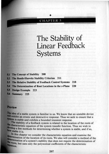
The Stability of Linear Feedback Systems

The Stability of
Linear Feedback
Systems
'"Be Concept of Stability 208
"he Routb-Hurwitz Stability Criterion 211
"he Relative Stability of Feedback Control Systems 218
"he Determination of Root Locations in the s-Plane 220
DeIIp Example 223
'-mary 225
ofa stable system is familiar to us. We know that an unstable device
I:Ihibit an erratic and destructive response. Thus we seek to ensure that a
is stable and exhibits a bounded transient response.
stability ofa feedback system is related to the location ofthe roots of
"'''''Clelristic equation of the system transfer function. Thus we wish to
a few methods for determining whether a system is stable, and if so,
Ilable it is.
In this chapter we consider the characteristic equation and examine the
"nation of the location ofits roots. We also will consider a method of the
ination ofa system's stability that does not require the determination of
~lS, but uses only the polynomial coefficients ofthe characteristic
On.
207

208 Chapter 5 The Stability of Linear Feedback Systems
III The Concept of Stability
The transient response of a feedback control system is of primary intere
must be investigat~d. A very. i.mportant characteristic of the transient ~;~
mance of a system IS the slabIllly of the system. A stable system is defined r.
system with a bounded system response. That is, if the system is subjected as a
bounded input or disturbance and the response is bounded in magnitude tQ~
system is said to be stable.
' t
The concept ofstability can be illustrated by considering a right circular co
pl.aced o~ a plane ho~zont.al.surface: ~ft~e cone i.s.resting .on its base and is tip~
~hgh~ly, It returns to Its ongmal equlhbn~m Osition .. Th~s position and response
Is.sald to be stable. If the cone re~t~ on 1tS. sld~ and I~ dlsp~a.ced slightly, it rolls
With no tendency to leave the posItion on ItS side. This positiOn is designated as
the neutral stability. On the other hand, if the cone is placed on its tip and
released, it falls onto its side. This position is said to be unstable. These three
positions are illustrated in Fig. 5.1.
The stability of a dynamic system is defined in a similar manner. The
response to a displacement, or initial condition, will result in either a decreasing,
neutral, or increasing response. Specifically, it follows from the definition Orstability
that a linear system is stable ifand only ifthe absolute value ofits impulse
response, g(l), integrated over an infinite range, is finite. That is, in terms orthe
convolution integral Eq. (4.1) for a bounded input, one requires that f~ Ig(I)J tit
be finite. The location in the s-plane ofthe poles ofa system indicate the resultina
transient response. The poles in the left-hand portion of the s-plane result in a
decreasing response for disturbance inputs. Similarly, poles on thejw-axis and in
the right-hand plane result in a neutral and an increasing response, resj)C{:tively,
for a disturbance input. This division of the s·plane is shown in Fig. 5.2. Clearly
the poles ofdesirable dynamic systems must lie in the left-hand portion of the 50
plane [20].
A common example ofthe potential destabilizing effect offeedback is that ~f
feedback in audio amplifier and speaker systems used for public address in a.udl o
toriurns. In this case a loudspeaker produces an audio signal that is an amphfi~
version of the sounds picked up by a microphone. In addition -to other a~dlo
inputs, the sound coming from the speaker itself may be sensed by the mICro-
'fl
____ ~--------Ci---------~ --
(al Slable
(b) Neutral
Figure S.t. The stability ofa cone.
(c) UnSlabk

5.1 The Concept of Stability
209
Stable
Neutral
Unstable
Figure 5.2. Stability in the s-plane.
How strong this particular signal is depends upon the distance between
speaker and the microphone. Because of the attenuating properties of
Iaqer this distance is, the weaker the sign~1 is that reaches the micro­
ID addition, due to the finite propagation s*ed of sound waves, there is
y between the signal produced by the lou~speaker and that sensed by
one. In this case, the output from the feedback path is added to the
input. This is an example of positive feedback.
the distance between the loud speaker and the microphone decreases, we
ifthe microphone is placed too close to the speaker then the system will
. The result ofthis instability is an excessive amplification and distoraf'audio
signals and an oscillatory squeal.
",otI>erexamp!e ofan unstable system is shown in Fig. 5.3. The flrst bridge
the Tacoma Narrows at Puget Sound, Washington, was opened to traffic
1.1940. The bridge was found to oscillate whenever the wind blew. After
!hI. on November 7,1940, a wind produced an oscillation that grew in
until the bridge broke apart. Figure 5.3(a) shows the condition of
oscillation; Fig. 5.3(b) shows the catastrophic failure [II].
1enns of linear systems, we recognize that the stability requirement may
in terms of the location of the poles of the closed-loop transfer funcclosed-loop
system transfer function is written as
KIt: I (s + Zi)
p(s)
T( .). - - (5.1)
q(s) s"'rr~_1 (s + O"k) II:_I [~ + 2u m s + (u;n + w;,,)] ,
1(&) • 4(s) is the characteristic equation whose roots are the poles of the
system. The output response for an impulse function input is then
c(t) = t. A k e- Ok1 + t B m (-!...) e-"",1 sin w",l (5.2)
k_1 m_1 W m
O. Clearly, in order to obtain a bounded response, the poles of the
GIld syst~m must ~ in the left-hand portion of the s-plane. Thus, a necnifficlent
conditIOn that afeedback system be stable is that a/1 the poles
em transfer function ha~'e negative real parts.

Figure 5.3(a}.
Figure S.J(b}. (Photos courtesy of F. B. Farquharson.)

5.2 The Routh·Hurwitz Stability Criterion 211
der to ascertain the stability of a feedback control system, one could
In ~re the roots of the characteristic equation q(s). However, we are first
deIt..nu~ in determining the answer to the question: "'s the system stable" If
iD1t::t late the roots of the characteristjc equation in order to answer this ques­
~ Cll have determined much more information than is necessary. Therefore,
IiCJIl. ~methods have been developed which provide th@ required "yes" or "no"
JIVCI'I.. 10 the stability question. The three approaches to the Question ofstability
~) The s-plane approach, (2) the frequency plane Uw) approach, and (3) the
~omain app~oach. The ~eal frequ~ncy (jw) ap~roach is oullin.ed in Chapter
..aad the discussion of the ttme·domalO approach IS deferred uniii Chapter 9.
• The Routh-Hurwitz Stability Criterion
']"be discussion and determination of stability has occupied the interest of many
_neers. Maxwell and Vishnegradsky first considered the question of stability
ofdynamic systems. In the late 1800s, A. Hurwitz and E. J. Routh published
iDdePendently a method of investigating the stability of a linear system [2, 3].
The Routh-Hurwitz stability method provides an answer to the Question of stability
by considering the characteristic equation of the system. The characteristic
equation in the laplace variable is written as
6(s) = q(s) = a"sn + on_Is"-1 + ... + ajs + au ::: O. (5.3)
III order to ascertain the stability ofthe system, it is necessary to determine ifany
of the roots of q(s) lie in thc right half of the s-plane. If Eq. (5.3) is written in
6ctored form, we have __
an(s - ,\)(s - (2) ..• (s - 'n) = 0, (5.4)
Where" ... ilh root ofthe characteristic cquation. Multiplying the factors togcther
we find that
'
q(s) = a"s" -
a"(rl + 'z + ... + 'n)s"-I
+ a.('I'2 + rZr J + 'I') +. .)s"-2
- a"(rl,Z') + 'Ir z ,.' •)sn-J +
L + an( -IY",z') . 'n = O.
All other Wo d l'.
r S, lor an nth-degree equation, we obtain
q(s) '"' a"s" -
an(sum of all the roots)s"-I
(5.5)
+ an(sum oflhe products of the roots taken 2 at a time)s"-z
- a"(sum ofthe products of the roots taken 3 at a time)s"-J
(5.6)
Eta + ... + a"(-!)"(product ofall II roolS) = O.
mining Eq (5 5) . .
e the same . '.' ,we note that .a11 the coeffiCients of the polynomial must
sign Ifall the roots are In the left-hand plane. Also, it is necessary

212 Chapler 5 The Stability of Linear Feedback Systems
for a stable system that all the coefficients be nonzero. However. although lh
requirements are necessary, they are not sufficient; that is, if1hey are not satisfi~
we immediately know the system is unstable. However, if they are satisfied Cd,
must. p~oceed t~ a~rtain the stability ofthe system. For example, when the Cha~
actenSile equatIon IS
q(s) - (s + 2)(.1' - s + 4) - (s' + .I' + 2s + 8),
(5.1)
the system is unstable and yet the polynomial possesses all positive coefficients
The Routh-Hurwitz crilerion is a necessary and sufficient criterion for the s~.
bitity of linear systems. The method was originally developed in terms of deter.
minants, but we shall utilize the more convenient array formulation.
The Routh-Hurwitz criterion is based on ordering the coefficients oflhe char.
acteristic equation
a,.s" + a.._Is"-1 + a.. _:5"-2 + ... + a,s + 00 = 0 (5.!)
into an array or schedule as follows [4):
~-, I
0.. a"_2 o.. _~
0 .. _1 a.._} a.._3
Then, further rows ofthe schedule are completed as follows:
"
s"
a.._2 o.. -~
r' 0 .. _1 °"_1 °"_5
r' b"_1 b"_ 3 b"_s
r' C"_I C"_J c.._s
where
and
(0...Xa. J - 0..(0.
b._I = ,) _-=..1-1.' ·'_'1
b"_ l = --- I I. " a"_~1
0 .. _ 1 0 .. _ 1
'
o.. _s
- Q._I 0._1 Q..-l •
C.. _ I = -- -I 1.'_' ·'_'1 ,
b.. _, b"_ 1 b"_ l
. . . be foJlo ....oed
and so on. The algorithm for calculating the entnes In the array can
on a determinant basis or by using the form ofthe equation for b.. _1• . h posi-
The Routh·Hunvilz crilerion slales lhat the number ofroots ofq(s) wit ((hi
lil·e real parts is equal to lhe number ofchanges in sig~ of.the flrsl co!lml~~urnl1
array. This criterion requires that there be no changes tn Sign tn t~e first
for a stable system. This requirement is both necessary and suffiCient.

5.2 The Routh-Hurwitz Stability Criterion
213
are three distinct cases that must be treated separately, requiring suit­
~tions ofthe array calculation procedure. The three cases are: (1) No
in the first column is zero; (2) there is a zero in the first column, but some
eIaJICflts oftbe row containing the zero in the first column are nonzero; and
isa zero in the first column, and the other e&ements ofthe row containing
are also zero.
order 10 clearly illustrate this method, several examples will be presented
.....
1. No element in the first column is zero.
q(s) = a~ + a2i + a,s + Gosa.p
Ie 5.1 Second-order system
....eteristic equatjon ofa second·order system is
q(s) >IE
b, = alllo-(O)Ol "" -I la, "'I ~ a,.
aj OJ a, 0
the requirement for a stable second.arder system is simply that all the
IS be positive_
Sa.pie S.2 Third-order system
dlaracteristic equation ofa third.arder system is
.r' OJ a l
i 02 ao
Sl b l
0
f C I 0
1be =ird~r~er
alr + als + Gob
_ a2a , - lloOl b llo
r - and CI = -'- - a,.
a2
system to be stable, it is necessary and sufficient that the coefpOSitive
and a2aj > QoOl- The condition when a)Ol = QoO) results in
b j

214 Chapter 5 The Stability of Linear Feedback Systems
a borderline stability case, and one pair ofroots lies on the imaginary axis i
s-plane. This borderline case is recognized as Case 3 be

5.2 The Routh·HuTWitz Stability Criterion
215
. ' desired to determine the gain K that results in borderline stability, The
.1. 15 . h
aurwitz array IS t en
s' 11K
s' 110
•
s' ,K 0
s' clOD
I' K 0 0
t - K -K
CI =-----
, ,
for any value of K greater than zero, the system is unstable. Also,
me last term in the first column is equal to K, a negative value of K will
in an unstable system, Therefore the system is unstable for all values of
L
3. Zeros in the first column, and the other elements of the row
g the zero are also zero.
3 occurs when all the elements in one row are zero or when the row
of a single element which is zero. This condition occurs when the
iaI contains singularities that are symmetrically located about the on·
of the s·plane. Therefore Case 3 occurs when factors such as
.Xs - If) or (s + jw)(s - jw) occur. This problem is circumvented by utithe
auxiliary equation, which immediately precedes the zero entry in the
amy. The order ofthe auxiliary equation is always even and indjcates the
ofsymmetrical root pairs.
order to illustrate this approach, let us consider a third-order system with
lIl""'ri"stic equation:
q(5) - s' + 2s' + 45 + K,
K is an adjustable loop gain. The Routh array is then
s' 1 4
s' 2 K
8 - K
Sl 2 0
I' K O.
re, for a stable system, we require that
o

216
Chapter 5 The Stability of Linear Feedback Systems
row preceding the row ofzeros is, in this case, obtained from the 5 1 -row. We
that this row contains the coefficients ofthe even powers ofs and therefore i~eca.1I
~~wehave ,
thIs
V(s) ~ 2s' + Ki' ~ 2s' + 8 ~ 2(s' + 4) ~ 2(s + j2)(s - j2). (5.13)
[0 order to show that the auxiliary equation, U(s), is indeed a factor of the h
acteristic equation, we divide q(s) by U(s) to obtain
car.
i's + 1
2s' + 8) s' + 2s' + 4s + 8
sJ + 45
2s' + 8
2s' + 8
Therefore, when K = 8, the factors of the characteristic equation arc
q(s) ~ (s + 2)(s + j2Xs - j2). (5.14)
0'.
• Example 5.4 Robot control
Let us consider the control of a robot arm as shown in Fig. 5.4. It is predicted
that there will be about 100,000 robots in service throughout the world by 1996
[6]. The robot shown in Fig. 5.4 is a six-legged micro robot system using highly
flexible legs with high gain controllers that may become unstable and oscillale.
Under this condition, we have the characteristic polynomial
The Routh-Hurwitz array is
q(s) = s' + l' + 4s' + 24s' + 3s + 63.
s'
l'
s'
s'
s'
Therefore the auxiliary equation is
1 4 3
21
o
1 24 63
-20 -60 0
63 0
o O.
(5.15)
V(s) = 21s' + 63 = 21(s' + 3) = 21(s + jV3)(s -jV3), (5. 16 )
which indicates that two roots are on the imaginary axis. In order to examine lhe
remaining roots, we divide by the auxiliary equation to obtain
~ = Sl + s2 + S + 21.
s'+3

5.2 The Routh-Hurwitz Stability Criterion
217
SA. A completely integrated, six-legged, micro robot system. The legged design
maximum dexterity. Legs also provide a unique sensory system for
tal interaction. It is equipped with a sensor network that includes 150
of 12 different types. The legs are instrumented so that it can determine the lay
IaTain, the surface texture, hardness, and even color. The gyro-stabilized camera
nder can be used for gathering data beyond the robot's immediatc reach. This
perfonnance system is able to walk quickly, climb over obstacles, and perform
• mOlions. Courtesy of IS Robotics Corporation.
"nga Routh-Hurwitz array for this equation, we have
s' 1 1
s2 I 21
Sl -20 0
f' 21 O.
~t.:abanges in sign in the first c:01umn indicate the presence of two roots in
nd plane, and the system IS unstable. The roots in the right-hand plane
- +1 ±jV6.
• a.PIe S.S Disk-drive control
disk-storag d . .
t . e eVlces arc used with IOOay's computers [17]. The data head
o ~lfferent psitions on th~ spinning disk and rapid, accurate response
block dtagram of a disk-storage data·head positioning system is

218
Chapter 5 The Stability of Linear Feedback Systems
R(,)~ Co""oll" H
De~ired + K(s +

5.3 The Relative Stability of Feedback Control Systems
219
"•
,
"
"
I
• ,
" "' ,,
'.
10
Figure 5.6. Root locations in the s-planc.
uation lie in the right halfof the s-plane. However, if the system satisfies
th_Hurwitz criterion and is absolutely stable, it is desirable to determine
;ve srabilily; that is, it is necessary to investigate the relative damping of
root ofthe characteristic equation. Thc relative stability ofa system may be
as the property that is measured by the relative settling times ofeach root
. ofroots. Therefore relative stability is represented by the real part ofeach
Thus root'! is relatively more stable than the roots,,, 'I as shown in Fig.
1be relative stability ofa system can also be defined in terms of the relative
coefficients f of each complex root pair and therefore in terms of the
ofresponse and overshoot instead ofsettling time.
Hence the investigation of the relative stability of each root is clearly necesbecause,
as we found in Chapter 4, the location of the closed-loop poles in
'"Plane determines the performance of the system. Thus it is imperative that
ioe:xamine the characteristic equation q(s) and consider several methods for
determination of relative stability.
use the relative stability of a system is dictated by the location of the
ofthe characteristic equation, a first approach using an s-plane formulation
extend the Routh-Hurwitz criterion to ascertain relative stability. This can
ply accomplished by utilizing a change of variable, which shifts the s-plane
in order to utilize the Routh-Hurwitz criterion. Examining Fig. 5.6, we notice
a ~ft of the vertical axis in the s-plane to -(11 will result in the roots 'I, 'I
on the shifted axis. The correct magnitude to shift the vertical axis
be btained on a trial-and-error basis. Then, without solving the fifth-order
iaI q(s), one may determine the real part of the dominant roots,,, 'I'
Example 5.6 Axis shift
the simple third-order characteristic equation
q(s) ~ s' + 4s' + 6s + 4. (5.17)
Y! one might shift the axis other than one unit and obtain a Routh-Hurwitz
\\>tth~ut a zero occurring in the first column. However, upon setting the
vanable Sn equal to s + I, we obtain
"
(5.18)

220 Chapter 5 The Stability of Linear Feedback Systems
Then the Routh array is established as
~ 1 1
S; 1 1
s~ 0 0
~ 1 O.
Clearly, there arc roots on the shifted Imaginary axis and the rOOls can be
obtained from the auxiliary equation, which is
U(s.) - S; + 1 - (s. + j)(s. - j)
_ (s+ 1 +j)(s+ 1 -j). (5.19)
The shifting ofthe s·plane axis in order to ascertain the relative stability of a
system is a very useful approach, particularly for higher-order systems with sev.
eral pairs ofclosed·loop complex conjugate roots.
III The Determination of Root Locations in the s-Plane
The relative stability of a feedback control system is directly related to the loca·
tion of the closed-loop roots of the characteristic equation in the s-plane. There·
fore it is often necessary and easiest to simply determine the values of the roots
of the characteristic equation. This approach has become particularly attractive
today due to the availability of digital computer programs for determining the
roots ofpolynomials. However, this approach may even be the most logical when
using manual calculations ifthe order ofthe system is relatively low. For a thirdorder
system or lower, it is usually simpler to utilize manual calculation methods.
The determination of the roots ofa polynomial can be obtained by utilizing
synlhelic dh>isioll which is based on the remainder theorem; that is, upon dividing
the polynomial by a factor, the remainder is zero when the factor is a root of the
polynomial. Synthetic division is commonly used to carry out the division p":
cess. The relations for the roots of a polynomial as obtained in Eq. (5.6) are utilized
to aid in the choice ofa first estimate of a root.
• Example 5.7 Synthetic division
Let us determine the roots ofthe polynomial
q(s) - s' + 45' + 6s + 4.
Establishing a table of synthetic division, we have
4 6 4 l=..! = trial rQot
-I -3 -3
(5.20)
3 3 = remainder

5.4 The Determination of Root Locations in the s-Plane
221
root of 5 = - I. In this table, we multiply by the trial root and succesadd
in each column. With a remainder ofone, we might try s = - 2, which
in the form
4 6 4 1-2
-2 -4 -4
2 2 0
the remainder is zero, one root is equal to - 2 and the remaining roots
obtained from the remaining polynomial (52 + 25 + 2) by using the qualOOt
formula.
search for a root ofthe polynomial can be aided considerably by utilizing
of change of the polynomial at the estimated root in order to obtain a
tllimate. The Newton-Raphson method is a rapid method utilizing synthetic
to obtain the value of
d~;) L"
II is a first estimate of the root. The Newton-Raphson method is an iterach
utilized in many digital computer root-solving programs. A new
SUI ofthe root is based on the last estimate as [I8, 19]
q(s.)
SHl = s~ - q'(S~)'
(5.21 )

222 Chapter 5 The Stability of Linear Feedback Systems
bm_ h ••• , hi coefficients. The value of q'(sn) is the remainder of this rcpe
synthetic division process. This process converges as the square of the abso~lect
error. The Ncwton-Raphson method, using synthetic division, is readily 'ttte
trated, as can be seen by repeating Example 5.7. I U$-
• E x amp I e 5.8 Newton-Raphson method
For the polynomial q(s) = 53 + 45 2 + 6$ + 4, we establish a table of sYnth t'
division for a first estimate as follows:
e Ie
4 6 4 l.=..!.
-I -3 - 3
3 3 = q(s,)
-I -2
2 = q'(s,)
The derivative of q(s) evaluated at $1 is determined by continuing the synthetic
division as shown. Then the second estimate becomes
s = s _ q(s,) = -I - (!) = - 2
2 I q '(51) I .
As we found in Example 5.7, $2 is, in fact, a foot ofthe polynomial and results in
a zero remainder.
• E x amp Ie 5.9 Third-order system
Let us consider the polynomial
q(s) = s' + 3.5s' + 6.5s + 10. (5.22)
From Eq. (5.6), we note that the sum of all the roots is equal to - 3.5 and thai
the product of all the roots is -10. Therefore, as a first estimate, we try 51 •
- I and obtain the following table:
3.5 6.5 10 l.=..!.
-I -2.5 -4
2.5 4 6 = q(s,)
-I -1.5
Therefore a second estimate is
52 = -I - (2~5) = -3.40.

5.5 Design Example: Tracked Vehicle Turning Control
223
let us use a second estimate that is convenient for these manual calculations.
re on the basis ofthe calculation of 52 "" - 3.40, we will choose a second
~ ;2 '"" - 3.00. Establishing a table for S2 = - 3.00 and completing the
'c division, we find that
q(s,) (- 5)
SJ = -S1 - q'(5z) = -3.00 - ili "" -2.60.
•completing a table for SJ "" - 2.50, we find that the remainder is zero and
poIyDomial factors are q(s) = ($ + 2.5)(s1 + $ + 4).
1be availability of a digital computer or a programmable calculator enables
10 readily determine the roots of a polynomial by using root determination
S, which usually use the Newton-Raphson algorithm, Eq. (5.21). This, as
case for time·shared computers with remote consoles, is a particularly use­
IPPfO&ch when a computer is. rea~ily avaiJable for immediate a~c.ess. The
. 'ty ofa console connected In a ttme·shared manner to a large digital comar
a personal computer is particularly advantageous for a control engineer,
the ability to perform on·line calculations aids in the iterative analysis
design process.
Design Example: Tracked Vehicle Turning Control
design ofa turning control for a tracked vehicle involves the selection oftwo
~~~[22l. In Fig. 5.7 the system shown in part (a) has the model shown in
(b). The two tracks are operated at different speeds in order to turn the vehi-
Track
torque
Power
train and
control
Right
loft
Vehicle
-
OJrection of
t!livel
C(s)
'.)
Diffefl:ncc in tTllC" speed
(.)
Po_r train
.,
vehicle G{s)
:s.'--~~-~__;:_;_HL_'_('_+_2~_('_+_"_~C(')
(b)
Filure 5.7. Turning control for a two-track vehicle.

224 Chapter 5 The Stability of Linear Feedback Systems
cle. Select K and a so that the system is stable and the steady-state errOr fo
ramp command is less than or equal to 24% of the magnitude of the comman~ a
The characteristic equation of the feedback system is .
or
Therefore we have
or
I + GcG(s) - 0
I + =="K",(s,-+~a!,-),--;-"""" 0
sis + 1Xs + 2)(s + 5) ~ .
sis + l)(s + 2)(s + 5) + K(s + a) ~ 0
(5.23)
s' + 8s' + 175' + (K + 10)s + Ka - O. (5.24)
In order to determine the stable region for K and a, we establish the Routh array
as
where
s' I 17 Ka
s' 8 K + 10 0
s' b, Ka
s' c,
s' Ka
b, = 126 - K and blK + 10) - 8Ka
8 c) = b
•
1
In order for the elements of the first column to be positive, we require that Kat
b), and c] be positive. Therefore we require
K < 126
(K+ IOXI26-K)-64Ka>0.
Ka > 0 (5.25)
The region ofstability for K > 0 is shown in Fig. 5.8. The steady-state error to a
ramp input r(t) = At, t > 0 is
where
Therefore we have
K~ = lim sGrG = Ka/IO.
~,
lOA
e"=Ka·
(5.26)

,
5.6 Summary
225
2
"
06
o
o
so 70
100 126 ISO
K
Figure 5.8. The stable region.
ell is equal to 23.8% of A, we require that Ka = 42. This can be satisfied
the selected point in the stable region when K = 70 and a = 0.6, as shown in
5.8. Of course, another acceptable design would be attained when K = 50
G - 0.84. We can calculate a series ofpossible combinations of K and a that
utisfy Ka = 42 that lie within the stable region, and all will be acceptable
solutions. However, not all selected values of K and a will lie within the
region. Note that K cannot exceed 126.
Summary
chapter we have considered the concept ofthe stability ofa feedback cont)'Item.
A definition ofa stable system in terms ofa bounded system response
':'Ottined and related to the location of the poles of the system transfer fune­
In the s-plane.
The Routh-Hurwitz stability criterion was introduced and several examples
~idered. The relative stability ofa feedback control system was also con­
• In terms ofthe location ofthe poles and zeros ofthe system transfer func­
~ the s-plane. Finally, the determination of the roots of the c-haracteristie
on was considered and the Newton-Raphson method was illustrated.
• A sYStem has a characteristic equation 5 l + 3Ks l
ofK for a stable system.
K :> 0.53
+ (2 + K)s + 4 = O. Determine

226 Chapler 5 The Stability of Linear Feedback Systems
E5.2. A system has a characteristic equalion 53 + 9$1 + 265 + 24 "" O. (a) U .
Routh criterion, show that the system is stable. (b) Using the Ncwton-Raphson Sing the
find Ihe three roots.
methOd,
ES.3. Find the roots of the characteristic equation s· + 9.5$J + 30.5s 1 + 37$ + 1') - • 0
E:S.4. A control system has the structure shown in Fig. E5.4. Determine Ihe gain at w ..
the system will become unstable.
hleh
Figure E5.4. Feedforward system.
E5.5. A feedback system has a loop transfer function
K
GH(s) = ($ + IXs + 3){s + 6)'
where K = 10. Find the roOIS of this system's characteristic equation.
E5.6. For the feedback system of Exercise E5.5, find thc value of K when two rOOIS lie on
the imaginary axis. Determine the value of the three roots.
Answer: s =
-10, ±j5.2
£5.7. A negative feedback system has a loop transfer function
GH(s) = K(s + 2)
s(s 2)·
(a) Find the value ofthe gain when the roflhe closed-loop roots is equal to 0.707. (b) Find
the value of the gain when the closed-loop system has two roots on the imaginary axis.
E5.8. Designers have developed small, fast, venical-takeofffighter aircraft that are invisible
to radar (Stealth aircraft). The aircraft concept shown in Fig. E5.8(a), on the next paIC
uses quickly tumingjet nozzles to steer the airplane 119]. The control syslem for the heading
or direction control is shown in Fig. E5.8(b). Determine the maximum gain of the
system for stable operation.
E5.9. A system has a characleristic equation
Find the range of K for a stable system.
sl + 3s2 + (K + I)s + 4 = 0
An.f~·er:
K > l'
E5.10. We all use our eycs and ears to achieve balance. Our orientation system allo.",S ~~
to sit or stand in a desired position even while in motion. This orientation system IS P Is
marily run by the information received in the inner ear, where the semicircular can a

Problems
227
(.)
Controlk,
--------
(b)
figun £5.8. Aircraft heading conlrol.
~C")
~ II,,',",
IIliplar acceleration and the otoliths measure linear acceleration. But these acceler­
.....urements need to be supplemented by visual signals. Try the following cxpcri­
(I) Stand with one foot in front ofanother and with your hands resting on your hips
dboW5 bowed outward. (b) Oose your eyes. Did you find that you experienced a
!!'I"'''' oscillation that grew until you lost balance Is this orientation position sta­
- without the use of your eyes'
Routh-Hurwitz criterion, dcterminc the stability of the following
(b) s) + 4s 1 + 5s + 6
(d) s' + r + 2.fl + 4s + 8
(f) s' + s' + 2s" +s + 3
eaacs, determine the number of roots, ifany, in the right-hand plane. Also, when it
ble, determine the range of K that results in a stable system.

228 Chapter 5 The Stability of Linear Feedback Systems
PS.2. An antenna control system was analyzed in Problem 3.5 and it was determined
in order to reduce the effect of wind disturbances, the gain of the magnetic amplifi thai
should be as large as possible. (a) Determine the limiting value of gain for maintai ~t k,
stab~e syster!l. (b) It is desired to ha.ve a ~ys~cm settling .time equal to two seconds. ~~ra
a shIfted aXIs and the Routh-Hurwllz cnlenon, determme the value of gain thaI sat' 6"1
this requirement. Assume that the complex fOOls of the closed-loop system dominal 1S ts
transient response. (Is this a valid approximation in Ihis case)
e 1!'It
PS.3. Arc welding is onc of the most important areas of application for industrial Tobo
[6]. In most manufacturing welding situations, uncertainties in dimensions of the Pa ls
geometry of the joint, and the welding process itself require the use of sensors for main.
taining weld quality. Several systems use a vision system to measure the geometry Oft~
puddle of melted metal as shown in Fig. P5.3. This system uses a constant rate offeedifl&
the wire to be melted. (a) Calculate the maximum value for K for the system that will rf1ult
in an oscillatory response. (b) For ~ of the maximum value of K found in part (a), deter.
mine the roots of the characteristic equation. (c) Estimate the overshoot of the system of
part (b) when it is subjected to a step input.
Desired
diamet~r
Controller
Wire-melting
process
A.
+ Error --L current 1
..I ,+2 (O.$s + t)(s + 1)
-
diameter """"
Vision ~y~t~m
M~asured
diameter 1
0.005s + 1
Figure PS.3. Welder control.
PS.4, A feedback control system is shown in Fig. P5.4. The process transfer function is
G(s) ~ K(s + 30) ,
s(s + 10)
and the feedback transfer function is H(s) :: I/(s + 20). (a) Determine the limiting v~ue
ofgain K for a stable system. (b) For the gain that results in borderline stability, detennt~
the magnitude of the imaginary roots. (c) Reduce the gain to ~ the magnitude ofth~ ~
derline value and determine the relative stability ofthe system (1) by shifting the aXIS ' tht
using the Routh-Hurwitz criterion and (2) by determining the root locations. ShoW
roots are between - I and - 2.
R(s)
1---..._ C(s)
Figure PS.4. Feedback system.

Problems
229
. the relative stability ofthe systems with the following characteristic cqua­
~Ii~ng the axis in the s-pla~e and using the Routh-Hurwitz criterion and (b)
~ ins the location of the rOOts In the s-plane:
+Jr+4s+2- 0
+t.r + lOs! + 42s + 20:: 0
+ t9r + 110$ + 200 - 0
unity-feedback control system is Sho;nfin Fi.&- P5.6. ,Dctc~minhe the rcla.tivchsta­
Ibe system with thc following !ranSlcr unctIOns by oeatmg t c roots In t c s-
65 + 335
)- ,'(,+ 9)
Figure PS.6. Unity fecdback systcm.
The linear model of a phase detector (phase-lock loop) can be represented by Fig.
Tbe phase-lock systems arc designed to maintain zero difference in phase between
carrier signal and a local voltage

230 Chapler 5 The Stability of Linear Feedback Systems
P5.8. A very interesting and useful velocity control system has been designed for a ~
chair control system [131. It is desirable to enable people paralyzed from'the neck d W ttl.
drive themselves about in motorized wheelchairs. A proposed system utilizing \lO~n.1a
sensors mounted in a headgear is shown in Fig. P5.8. The headgear sensor provi~ OClty
output proportional to the magnitude orlhe head movement. There is a sensor rno es an
at 90· intervals so that forward, left, right, or reverse can be commanded. Typical v~~led
for the lime constants are TI "" 0.5 sec, Tl = I sec, and T. = Yo sec. (a) Determin lles
limiting gain K = K,KlK J for a stable system. (b) When the gain K is set equal to MoCr the
limiting value. determine if the settling lime of the system is less than 4 sec. (c) Deterrn~
the value ofgain that results in a system with a settling time of4 Set. Also, obtain Ihe v~ne
of the roots of the characteristic equation when the settling time is equal to 4 sec. lie
Desired
velocity
+
Amplifier
Wheelchair
dynamics
Figure P5.8. Wheelchair control system.
PS.9. A cassette tape storage device has been designed for mass-storage (13]. [I is necessal)
to control accurately the velocity of the tape. The speed control of the tape drive is represented
by the system shown in Fig. P5.9. (a) Determine the limiting gain for a stable system.
(b) Determine a suitable gain so that the overshoot to a step command is approximately
5%.
Power
amplifier
'1__,~+_K_l_00~_H
Motor and
drive mechanism
(, ;'W)' ~s~
Figure P5.9. Tape drive conlrol.
.' . '- ceurale, fas
PS.IO. Robots can be used L
In manufactunngand assembly operatIOns w"ere a d'rect"
and versatile manipulation is required (9]. The open-loop transfer function of a t
drive arm may be approximated by
K(s + 2)
GH(s) "" s(s + 5X.r + 2s + 5)
tS oft!Je
(a) Determine the value ofgain Kwhen the system oscillates. (b) Calculate the rOO
closed-loop system for the K determined in part (a).

Problems
231
A (c:edback control system has a chal1lcteristic equation:
s' + (4 + J()r + 6s + 16 + 8X - O.
...."""'K must be positive. What is the maximum value K can assume before the
beCOmes unstable When K is equal 10 the maximum value, the system oscillates.
. the frequency of oscillation.
A feedback control system has a characteristic equalion:
f' + 2s' + 5s' + 8s' + 8sl + 8s + 4 + O.
ifthe system is stable and determine the values of the roots.
The stability ofa motorcycle and rider is an important area for study because many
designs result in vehicles that are difficuh to control (10). The handling char-
• ofa motorcycle must include a model of the rider as well as one ofthe vehicle.
4J8amics of one motorcycle and rider can be represented by an open-loop tl1lnsfer
(...... P5,4)
K(r + lOs + 1125)
GH(s) - s(s + 20)(.r + lOs + I 25)(.r + 60s + 34(0) .
ID approximation, calculate the acceptable I1lnge of K for a stable system when the
polynomial (zeros) and the denominator polynomial (Sl + 60s + 34(0) are
(b) Calculate the actual range ofacceptable K accounting for all zeros and poles.
A s)'!tem has a transfer function
T( ) I
s :::: r+ 1.3.r+ 2.0s + I'
ioe ifthe system is stable. (b) Determine the roots ofthe characteristic equation.
the response of the system to a unit step input.
Problems
•
The contr~l
of the spark ignilion of an automotive engine requires constant per­
-.~ver a W1~e range ofparam.eters (21]. The control system is shown in Fig. DP5.1,
IUtoIpage With a controller gam K to be selected. The parameter p is, equal to 2 for
.... but can equal zero for high performance autos. Select a gain K that will result
Iystem for both values ofp.
~ automatically guided vehicl~ on Mars is represented by the system in Fig..
_ .5YSIem has a steerable wheelm both the front and back ofthe vehicle and the
"-tUires th I '
for .~ se ectlon of H(s) where H(s) - Ks + I. Determine (a) the value of K
10 I • ~blllty, (b) the value of K when one rool of the characteristic equation is
"-cI1he'lt, and (c) the value of the t.....o remaining roolS for the gain selected in part
response ofthe system to a step command for the gain selected in part (b).

232 Chapter 5 The Stability of Linear Feedback Systems
!,
+
R(J)--o{
_,_ L...,..,-I -'-
1+5 I s+p
!
,
Figure DPS." Automobile engine control.
R(s>
Sleering
commarld
• +.0- -'-
,
,+'
i'
C(s)
Dirtttioo of
lra,'e1
H(J)
Figure DPS.2. Mars guided vehicle control.
DPS.3. A unity negative feedback system with
G(,) _ K(s + 2)
- s(l + T5)(1 + 25)
has two parameters to be selected. (a) Determine and plot the regions of stability for Ihis
system. (b) Select T and K so that the ready state error to a ramp input is less than or equal
to 25% of the input magnitude. (e) Determine the percent overshoot for a step input fot
the design selected in part (b).
DPS.4. The attitude control system of a space shuttle rocket is shown in Fig. DP5A [4).
(a) Determine the range of gain K and parameter In so that the system is stable and pial
the region ofstability. (b) Select the gain and parameter values so that the steady-state error
to a ramp input is less than or equal to 10% of the input magnitude. (e) Determine tbe
percent overshoot for a step input for the design selected in part (b).
..
Space SllUtlle
contro or ~,
R(s)
V-
Is
"
, ~-I
+ mXs + 2) Thrusl K
Anilude
C(s)
Figure DPS.4. Shuttle attitude control.

References
233
equation The equation that immediately precedes the zero entry in the
_yo
RapllsOn method An iterative approach to solving for roots of a poly.
equation.
stability The property that is m~as.ured by. the relative settling times of
*GOt or pair of roots ofthe charactenstlc cQuatlon.
Hanritz criterion A criterin for determining the ~tability of.a srstem by
., the characteristic equation ofthe transfcr function. The cntenon states
1be number of roots of the characteristic equation with positive real parts is
10 the number of changes of sign of the coefficients in the first column of
th array.
A perfonnance measure ofa system. A system is stable if all the poles
transfer function have negative real parts.
•ystem A dynamic system with a bounded system response to a bounded
division A method ofdetermining the roots of the characteristic eQuabued
on the remainder theorem of mathematics.
..C. Dorf, Introduction 10 Eleclric Circuirs. John Wiley & Sons, New York, 1989.
A. Hurwitz, "On the Conditions Under Which an Equation Has Only Roots with Negve
Real Parts," Mathemarische Annalen, 46, 1895; pp. 273-84. Also in Selected
on Mathematical Trends in Control Thear)'. Dover, New York, 1964; pp. 70-
J. Routh, Dynamics ofa S)'stem ofRigid Bodies, Macmillan, New York, 1892.
DeMeis, "Shuttling to the Space Station," Aerospace America. March 1990; pp. 44-
V. Rinswood, "Shape Control in Scndzimir Mills Using Roll Actuators," IEEE
ions on Automatic Conlrol. April 1990; pp. 453-59.
The SCIence ofTelecommUfllcatJOllS, W. H. Freeman, San Fran­
.i: ~rf, En.cyclopedia of~oborics, John Wiley.& s,ons, New York, 1988.
r;iao.~,Slgnals:
a 1990.
I. ri::::~' Large-Sc~/eSystems COlllrol, Marcel Dekker, New York, 1990.
F: Ita • Mtthatronlcs for Robots," Mechanical Engineering, July 1990; pp. 40-42.
,: B. ~n, Automatic Control Engineering, 2nd ed., McGraw-Hill, New York, 1990.
--.- arquharson, "Aerodynamic Stability of Suspension Bridges, with Special Ref­
'-ern ~o I~e Tacoma Narrows Bridge," Bullerin 116. Pari I, The Engineering Exper­
C. Do~on, Unive~sity of Washington, 1950.
So F' In~rodllclJOn10 Complllers and Compuler Science, 3rd cd.. Boyd and Fm­
C. 1'1 ranclSCO, 1982.
• Krause, Electromechanical Motioll Devices, McGraw.Hill, New York, 1989.

234 Chapter 5 The Stability of Linear Feedback Systems
14. R. C. Rosenberg and D. C. Kllrnopp, Introduction 10 Physical System D .
McGraw-Hill, New York, 1987.
('sign
15. T. Yoshikawa, Foundations ofRobotics. M.LT. Press, Cambridge, Mass., 1990.
16. B. E. Jeppscn, "A New Family of Dot Matrix Line Printers," HP Journal, June 198 .
p~~9. ~
17. R. E. Ziemer, Signals and Syswns. 2nd cd .. Macmillan, New York. 1989.
18. R. C. Dorfand R. Jacquot, Control System Design Program, Addison-Wesley R ad
ing, Mass., 1988. ' e .
19. R. A. Hammond, "Fly by Wire Control Systems," Simulation, October 1989; PP. 159­
67.
20. P. P. Vardyanathan and S. K. Mitra, "A Unified Struclurallnterprctation ofSo m
Well Known Stability Test Procedures for Linear Systems," Proceedings ofthe lEE;
November 1989; pp. 478-79. .
21. P. G. Scotson, "Self-Tuning Optimization of Spark Ignition Automotive Engines,"
IEE£ Control Srstems. April 1990; pp. 94-99.
22. G. G. Wang, "Design of Turning Control for a Tracked Vehicle," IEEE COlltrol SYj_
terns. April 1990; pp. 122-25.
23. A. Dane, "Hubble: Heartbreaks and Hope," Popular Mechanics. October 1990: pp.
130-31.
24. T. Beardsley, "Hubble's Legacy," Scientific American. Junc 1990; pp. 18-19.
25. C. Phillips and R. Harbor, Feedback Comrol Systems. Prentice Hall. Englewood Cliffs,
N.J., 1991.