The Stability of Linear Feedback Systems
The Stability of Linear Feedback Systems
The Stability of Linear Feedback Systems

Create successful ePaper yourself
Turn your PDF publications into a flip-book with our unique Google optimized e-Paper software.
5.1 <strong>The</strong> Concept <strong>of</strong> <strong>Stability</strong><br />
209<br />
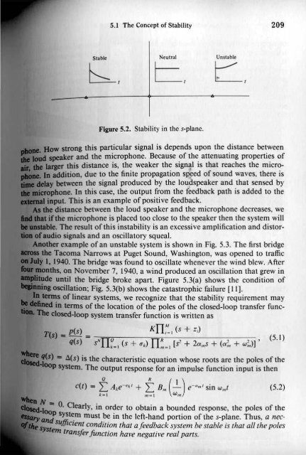
Stable<br />
Neutral<br />
Unstable<br />
Figure 5.2. <strong>Stability</strong> in the s-plane.<br />
How strong this particular signal is depends upon the distance between<br />
speaker and the microphone. Because <strong>of</strong> the attenuating properties <strong>of</strong><br />
Iaqer this distance is, the weaker the sign~1 is that reaches the micro<br />
ID addition, due to the finite propagation s*ed <strong>of</strong> sound waves, there is<br />
y between the signal produced by the lou~speaker and that sensed by<br />
one. In this case, the output from the feedback path is added to the<br />
input. This is an example <strong>of</strong> positive feedback.<br />
the distance between the loud speaker and the microphone decreases, we<br />
ifthe microphone is placed too close to the speaker then the system will<br />
. <strong>The</strong> result <strong>of</strong>this instability is an excessive amplification and distoraf'audio<br />
signals and an oscillatory squeal.<br />
",otI>erexamp!e <strong>of</strong>an unstable system is shown in Fig. 5.3. <strong>The</strong> flrst bridge<br />
the Tacoma Narrows at Puget Sound, Washington, was opened to traffic<br />
1.1940. <strong>The</strong> bridge was found to oscillate whenever the wind blew. After<br />
!hI. on November 7,1940, a wind produced an oscillation that grew in<br />
until the bridge broke apart. Figure 5.3(a) shows the condition <strong>of</strong><br />
oscillation; Fig. 5.3(b) shows the catastrophic failure [II].<br />
1enns <strong>of</strong> linear systems, we recognize that the stability requirement may<br />
in terms <strong>of</strong> the location <strong>of</strong> the poles <strong>of</strong> the closed-loop transfer funcclosed-loop<br />
system transfer function is written as<br />
KIt: I (s + Zi)<br />
p(s)<br />
T( .). - - (5.1)<br />
q(s) s"'rr~_1 (s + O"k) II:_I [~ + 2u m s + (u;n + w;,,)] ,<br />
1(&) • 4(s) is the characteristic equation whose roots are the poles <strong>of</strong> the<br />
system. <strong>The</strong> output response for an impulse function input is then<br />
c(t) = t. A k e- Ok1 + t B m (-!...) e-"",1 sin w",l (5.2)<br />
k_1 m_1 W m<br />
O. Clearly, in order to obtain a bounded response, the poles <strong>of</strong> the<br />
GIld syst~m must ~ in the left-hand portion <strong>of</strong> the s-plane. Thus, a necnifficlent<br />
conditIOn that afeedback system be stable is that a/1 the poles<br />
em transfer function ha~'e negative real parts.


![[Language - English] - Life Skills - Writing](https://img.yumpu.com/44143758/1/190x245/language-english-life-skills-writing.jpg?quality=85)