Modular-Based Modelling of Protein Synthesis Regulation
Modular-Based Modelling of Protein Synthesis Regulation
Modular-Based Modelling of Protein Synthesis Regulation

You also want an ePaper? Increase the reach of your titles
YUMPU automatically turns print PDFs into web optimized ePapers that Google loves.
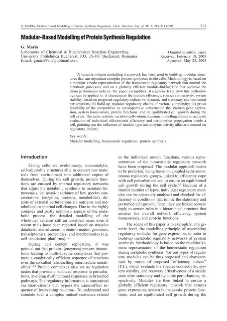
G. MARIA, <strong>Modular</strong>-<strong>Based</strong> <strong>Modelling</strong> <strong>of</strong> <strong>Protein</strong> <strong>Synthesis</strong> <strong>Regulation</strong>, Chem. Biochem. Eng. Q. 19 (3) 213–233 (2005) 213<br />
<strong>Modular</strong>-<strong>Based</strong><strong>Modelling</strong><strong>of</strong><strong>Protein</strong><strong>Synthesis</strong><strong>Regulation</strong><br />
G. Maria<br />
Laboratory <strong>of</strong> Chemical & Biochemical Reaction Engineering<br />
University Politehnica Bucharest; P.O. 35-107 Bucharest, Romania<br />
Email: gmaria99m@hotmail.com<br />
Original scientific paper<br />
Received: February 18, 2005<br />
Accepted: May 25, 2005<br />
A variable-volume modelling framework has been used to build-up modular structures<br />
that can reproduce complex protein syntheses inside cells. Methodology is based on<br />
a modular kinetic representation <strong>of</strong> the homeostatic regulatory network that control the<br />
metabolic processes, and on a globally efficient module-linking rule that optimise the<br />
chain performance indices. The paper exemplifies, at a generic level, how this methodology<br />
can be applied to: i) characterize the module efficiency, species connectivity, system<br />
stability, based on proposed regulatory indices vs. dynamic and stationary environmental<br />
perturbations; ii) build-up modular regulatory chains <strong>of</strong> various complexity; iii) prove<br />
feasibility <strong>of</strong> the cooperative vs. uncooperative construction that ensures gene expression,<br />
system homeostasis, proteic functions, and an equilibrated cell growth during the<br />
cell cycle. The more realistic variable-cell-volume dynamic modelling allows an accurate<br />
evaluation <strong>of</strong> individual effector/unit efficiency and perturbation propagation inside a<br />
cell, pointing out the influence <strong>of</strong> module type and enzyme activity allosteric control on<br />
regulatory indices.<br />
Key words:<br />
<strong>Modular</strong> modelling, homeostatic regulation, protein synthesis<br />
Introduction<br />
Living cells are evolutionary, auto-catalytic,<br />
self-adjustable structures able to convert raw materials<br />
from environment into additional copies <strong>of</strong><br />
themselves. During the cell growth, protein functions<br />
are ensured by internal regulatory networks<br />
that adjust the metabolic synthesis to maintain homeostasis,<br />
i.e. quasi-invariance <strong>of</strong> key species concentrations<br />
(enzymes, proteins, metabolites), despite<br />
<strong>of</strong> external perturbations (in nutrients and metabolites)<br />
or internal cell changes. Due to the highly<br />
complex and partly unknown aspects <strong>of</strong> the metabolic<br />
process, the detailed modelling <strong>of</strong> the<br />
whole-cell remains still an unsettled issue, even if<br />
recent trials have been reported based on massive<br />
databanks and advances in bioinformatics, genomics,<br />
transciptomics, proteomics, and metabolomics (e.g.<br />
cell simulation platforms). 1,2<br />
During cell content replication, it was<br />
pointed-out that proteins (enzymes) present interactions<br />
leading to multi-enzyme complexes that promote<br />
a catalytically efficient sequence <strong>of</strong> reactions<br />
over the so-called ‘channelling intermediate metabolites’.<br />
3,4 Proteic complexes also act as regulation<br />
nodes that provide a balanced response to perturbations,<br />
avoiding dysfunctional responses in branched<br />
pathways. The regulatory information is transmitted<br />
via short-circuits that bypass the cause-effect sequence<br />
<strong>of</strong> intervening reactions. To understand and<br />
simulate such a complex mutual-assistance related<br />
to the individual proteic functions, various representations<br />
<strong>of</strong> the homeostatic regulatory network<br />
have been proposed. The modular approach seems<br />
to be preferred, being based on coupled semi-autonomous<br />
regulatory groups, linked to efficiently cope<br />
with cell perturbations and to ensure an equilibrated<br />
cell growth during the cell cycle. 4,5 Because <strong>of</strong> a<br />
limited number <strong>of</strong> types, individual regulatory modules<br />
can be separately analysed and checked for efficiency<br />
in conditions that mimic the stationary and<br />
perturbed cell growth. Then, they are linked accordingly<br />
to certain rules in a hierarchical structure that<br />
ensures the overall network efficiency, system<br />
homeostasis, and protein functions.<br />
The scope <strong>of</strong> this paper is to exemplify, at a generic<br />
level, the modelling principle <strong>of</strong> assembling<br />
regulatory modules for gene expression, in order to<br />
build-up metabolic regulatory networks <strong>of</strong> protein<br />
synthesis. Methodology is based on the modular kinetic<br />
representation <strong>of</strong> the homeostatic regulation<br />
during metabolic synthesis. Various types <strong>of</strong> regulatory<br />
modules can be thus proposed and characterized<br />
by means <strong>of</strong> proposed “efficiency indices”<br />
(P.I.), which evaluate the species connectivity, system<br />
stability, and recovery effectiveness <strong>of</strong> a steady<br />
state after stationary and dynamic perturbations, respectively.<br />
Modules are then linked to ensure a<br />
globally efficient regulatory network that ensures<br />
gene expression, system homeostasis, proteic functions,<br />
and an equilibrated cell growth during the
214 G. MARIA, <strong>Modular</strong>-<strong>Based</strong> <strong>Modelling</strong> <strong>of</strong> <strong>Protein</strong> <strong>Synthesis</strong> <strong>Regulation</strong>, Chem. Biochem. Eng. Q. 19 (3) 213–233 (2005)<br />
cell cycle. The paper exemplifies how such a methodology<br />
should be used to step-by-step build-up<br />
a regulatory chain, and how the feasibility and effectiveness<br />
<strong>of</strong> the (cooperatively-linked) modular<br />
construction can be checked in every modelling<br />
step by means <strong>of</strong> P.I.-s.<br />
The modelling framework uses continuous-variable<br />
ordinary differential (ODE) kinetic<br />
models to check the synthesis regulatory efficiency,<br />
by explicitly accounting for cell-volume variation<br />
during the cell cycle, protein interactions and regulatory<br />
loops under stationary and dynamic environmental<br />
perturbations. The more realistic modelling<br />
approach allows an accurate evaluation <strong>of</strong> the individual<br />
effector/unit relative importance, perturbation<br />
propagation inside a cell, and the influence <strong>of</strong><br />
module type and enzyme activity allosteric control<br />
on its regulatory P.I.-s. Once the methodology elaborated,<br />
such a cell modelling platform can be detailed<br />
and used to simulate complex protein / species<br />
interactions, cooperative regulation <strong>of</strong> the<br />
metabolic synthesis, and other processes during the<br />
cell growth.<br />
<strong>Modelling</strong> metabolic regulation –<br />
A short review<br />
<strong>Protein</strong> synthesis by gene expression is a<br />
highly regulated process which ensure a balanced<br />
and flexible cell growth under an indefinitely<br />
variate environmental conditions. How this very<br />
complex process occurs is partially understood, but<br />
a multi-cascade control with negative feedback<br />
loops seems to be the key element. 6–9 Enzymes<br />
catalysing the synthesis are allosterically regulated<br />
by means <strong>of</strong> positive or negative effector molecules,<br />
while cooperative binding and structured cascade<br />
regulation amplify the effect <strong>of</strong> a change in a<br />
signal. Gene expression is also highly regulated to<br />
flexibly respond to the environmental stress, in a<br />
scheme looking like a ‘genetic circuit’. 10 While the<br />
effect <strong>of</strong> changes in system parameters on the system<br />
states (variables) is approached by the metabolic<br />
control analysis, the metabolic regulator features<br />
are determined by its ability to efficiently vary<br />
species flows and concentrations under changing<br />
environmental conditions so, that a stationary state<br />
<strong>of</strong> the key metabolite concentrations can be maintained<br />
inside the cell.<br />
To model such a complex metabolic regulatory<br />
mechanisms at a molecular level, two main approaches<br />
have been developed over decades: structure-oriented<br />
analysis, and dynamic (kinetic) models.<br />
11 Each theory presents strengths and shortcomings<br />
in providing an integrated predictive description<br />
<strong>of</strong> the cellular regulatory network.<br />
Structure-oriented analyses ignore some mechanistic<br />
details and the process kinetics, and use the<br />
only network topology to quantitatively characterize<br />
to what extent the metabolic reactions determine<br />
the fluxes and metabolic concentrations. 12 The<br />
so-called ‘metabolic control analysis’ (MCA) is focus<br />
on using various types <strong>of</strong> sensitivity coefficients<br />
(the so-called ‘response coefficients’), which<br />
are quantitative measures <strong>of</strong> how much a perturbation<br />
(influential variable x j ) affects the cell-system<br />
states y i (e.g. r = reaction rates, J = fluxes, c = concentrations)<br />
around the steady-state (QSS, <strong>of</strong> index<br />
‘s’), i.e.( yi/ yis)/( x j/ x js) .<br />
The systemic response<br />
<strong>of</strong> fluxes or concentrations to perturbation<br />
s<br />
parameters (i.e. the ‘control coefficients’), or <strong>of</strong> reaction<br />
rates to perturbations (i.e. the ‘elasticity coefficients’)<br />
have to fulfil the ‘summation theorems’,<br />
which reflect the network structural properties, and<br />
the ‘connectivity theorems’ related to the properties<br />
<strong>of</strong> single enzymes vs. the system behaviour.<br />
Originally, MCA has been introduced by<br />
Kacser & Burns, 13 Heinrich & Rapoport, 14 and<br />
Burns et al. 15 to quantify the rate limitation in complex<br />
enzymatic systems. MCA have been followed<br />
by a large number <strong>of</strong> improvements, mainly dealing<br />
with the control analysis <strong>of</strong> the stationary states, by<br />
pointing-out the role <strong>of</strong> particular reactions and cell<br />
components in determining certain metabolic behaviour.<br />
Successive extensions <strong>of</strong> such definitions<br />
allow: to study any limit set for non-steady/time-dependent<br />
conditions; 16,17 the flux balance analysis<br />
and optimization (FBA); 11,12,18–22 elementary mode<br />
analysis (EMA); 11,18,19 dynamic flux balance analysis<br />
(DFBA); 23 extreme pathway analysis (ExPA); 18,19<br />
constrained based modelling <strong>of</strong> metabolic network<br />
(CBM). 24<br />
MCA methods are able to efficiently characterize<br />
the metabolic network robustness and functionality,<br />
linked with the cell phenotype and gene regulation.<br />
MCA allows a rapid evaluation <strong>of</strong> the system<br />
response to perturbations (especially <strong>of</strong> the enzymatic<br />
activity), possibilities <strong>of</strong> control and self-regulation<br />
for the whole path or some subunits. Functional<br />
subunits are metabolic subsystems, called<br />
‘modules’, such as amino acid or protein synthesis,<br />
protein degradation, mitochondria metabolic path,<br />
etc. 25 Because the living cells are self-evolutive systems,<br />
new reactions recruited by cells together with<br />
enzyme adaptations, can lead to an increase in the<br />
cell biological organisation and to optimal performance<br />
indices. When constructing methods to optimize<br />
evolutive metabolic systems, MCA concepts<br />
and appropriate performance criteria have been<br />
used to: maximize reaction rates and steady-state<br />
fluxes; minimize metabolic intermediate concentrations;<br />
minimize transient times; optimise the reac-
G. MARIA, <strong>Modular</strong>-<strong>Based</strong> <strong>Modelling</strong> <strong>of</strong> <strong>Protein</strong> <strong>Synthesis</strong> <strong>Regulation</strong>, Chem. Biochem. Eng. Q. 19 (3) 213–233 (2005) 215<br />
tion stoichiometry (network topology); maximize<br />
thermodynamic efficiency. All these objectives are<br />
subjected to various mass balance, thermodynamic,<br />
and biological constraints. 12 However, by not accounting<br />
for the system dynamics, and grounding<br />
the analysis on the linear system theory, topological<br />
methods present inherent limitations (see for instance<br />
some violations <strong>of</strong> stoichiometric constraints<br />
discussed by Atauri et al., 26 or the modified control<br />
coefficients <strong>of</strong> Szedlacsek et al. 27,28 ).<br />
Classical approach to develop dynamic models<br />
is based on an hypothetical reaction mechanism, kinetic<br />
equations, and known stoichiometry. This route<br />
meets difficulties when the analysis is expanded to<br />
large-scale metabolic networks, because the necessary<br />
mechanistic details and standard kinetic data to<br />
derive the rate constants are difficult to be obtained.<br />
However, advances in genomics, transcriptomics,<br />
proteomics, and metabolomics, lead to a continuous<br />
expansion <strong>of</strong> bioinformatic databases, while advanced<br />
numerical techniques, non-conventional estimation<br />
procedures, and massive s<strong>of</strong>tware platforms<br />
reported progresses in formulating reliable cell models.<br />
Valuable structured dynamic models, based on<br />
cell biochemical mechanisms, have been developed<br />
for simulating various (sub)systems, such as:<br />
– entire cell: ‘whole-cell’ models, as E-Cell,<br />
V-Cell, M-Cell, A-Cell, etc.; 1<br />
– single cell growth: Escherichia coli; 29–31<br />
Haemophilus influenzae; 18,19 Mycoplasma genitalium;<br />
32–34 yeast; 35,36<br />
– various (oscillatory) metabolic paths: metabolism<br />
<strong>of</strong> human red blood cells; 36,37 glycolysis, citric<br />
acid cycle, oxidative phosphorylation 12,38–40 ; iron<br />
metabolism; 41 amino acid synthesis; 20<br />
– regulatory networks for: gene expression via<br />
Boolean ‘biocircuit’ models (Escherichia coli; 42,43<br />
prokaryotes; 44,45 protein synthesis 1,5,9 );<br />
– cell cycles and oscillatory systems in yeast<br />
and eukaryotes: limit-cycle oscillator models; 46–48<br />
cell size control, oscillation properties and hysteresis<br />
effects; 49 key ingredients inducing oscillations;<br />
49–55 whole-cell framework for cell cycle simulation;<br />
56<br />
– cellular communications, intracellular signalling,<br />
neuronal transmission, networks <strong>of</strong> nerve<br />
cells; 57–59<br />
– analysis <strong>of</strong> “logical essence” <strong>of</strong> life, and the<br />
life fundamental requirements. 60<br />
To model in detail the cell process complexity<br />
is a challenging and difficult task. The large number<br />
<strong>of</strong> inner cell species, complex regulatory chains,<br />
cell signalling, motility, organelle transport, gene<br />
transcription, morphogenesis and cellular differentiation<br />
cannot easily be accommodated into existing<br />
computer frameworks. Inherently, any model represents<br />
a simplification <strong>of</strong> the real phenomenon,<br />
while relevant model parameters are estimated<br />
based on the how close the model behaviour is to<br />
the real cell behaviour. A large number <strong>of</strong> s<strong>of</strong>tware<br />
packages have been elaborated allowing the kinetic<br />
performance <strong>of</strong> enzyme pathways to be represented<br />
and evaluated quantitatively. 61 Oriented and unified<br />
programming languages have been developed<br />
(CellML; 62 SBML 61 ) to include the bio-system organization<br />
and complexity in integrated platforms<br />
for cellular system simulation (E-Cell; 32,33 V-Cell; 63,64<br />
M-Cell; 58 A-Cell 59 ). Such integrated simulation<br />
platforms tend to use a large variety <strong>of</strong> biological<br />
databanks including enzymes, proteins and genes<br />
characteristics together with metabolic reactions<br />
(CRGM-database; 65 NIH-database 66 ).<br />
From the mathematical point <strong>of</strong> view, various<br />
structured (mechanism-based) dynamic models<br />
have been proposed to simulate the metabolic regulation,<br />
accounting for continuous, discrete, and/or<br />
stochastic variables, in a modular construction, ‘circuit-like’<br />
network, or compartmented simulation<br />
platforms. 1,2,67 Such models can include:<br />
– Boolean (discrete) variables; 10,44,68–70<br />
– continuous variable models; 9,12,68,71<br />
– stochastic variable models; 45,57,72,73<br />
– mixed variable models. 68<br />
In the Boolean approach, variables can take<br />
only discrete values. Even if less realistic, such an<br />
approach is computationally tractable, involving<br />
networks <strong>of</strong> genes that are either “on” or “<strong>of</strong>f” (e.g.<br />
a gene is either fully expressed or not expressed at<br />
all) according to simple Boolean relationships, in a<br />
finite space. Such a coarse representation is used to<br />
obtain a first model for a complex biosystem including<br />
a large number <strong>of</strong> components, until more<br />
detailed data on process dynamics become available.<br />
‘Electronic circuits’ structures have been extensively<br />
used to understand intermediate levels <strong>of</strong><br />
regulation, but they cannot reproduce in detail molecular<br />
interactions with slow and continuous<br />
responses to perturbations.<br />
Even if regulation mechanisms are not fully<br />
understood, metabolic regulation at a low-level is<br />
generally better clarified. <strong>Based</strong> on that, conventional<br />
dynamic models (ODE kinetics), with a<br />
mechanistic description <strong>of</strong> reactions taking place<br />
among individual species (proteins, mRNA, intermediates,<br />
etc.) have been proved to be a convenient<br />
route to analyse continuous metabolic/regulatory<br />
processes and perturbations. When systems are too<br />
large or poorly understood, coarser and more<br />
phenomenological kinetic models may be postulated<br />
(e.g. protein complexes, metabolite channelling,<br />
etc.). In dynamic models, only essential reactions<br />
are retained, the model complexity depending
216 G. MARIA, <strong>Modular</strong>-<strong>Based</strong> <strong>Modelling</strong> <strong>of</strong> <strong>Protein</strong> <strong>Synthesis</strong> <strong>Regulation</strong>, Chem. Biochem. Eng. Q. 19 (3) 213–233 (2005)<br />
on measurable variables and available information.<br />
An important problem to be considered is the distinction<br />
between the qualitative and quantitative<br />
process knowledge, stability and instability <strong>of</strong> involved<br />
species, the dominant fast and slow modes<br />
<strong>of</strong> process dynamics, reaction time constants, macroscopic<br />
and microscopic observable elements <strong>of</strong><br />
the state vector. Such kinetic models can be useful<br />
to analyse the regulatory cell-functions, both for<br />
stationary and dynamic perturbations, to model cell<br />
cycles and oscillatory metabolic paths, 56 and to reflect<br />
the species interconnectivity or perturbation<br />
effects on cell growth. 74 Mixtures <strong>of</strong> ODE kinetics<br />
with discrete states (i.e. ‘continuous logical’ models),<br />
and <strong>of</strong> continuous ODE kinetics with stochastic<br />
terms, can lead to promising mixed models able<br />
to simulate, both, deterministic and non-deterministic<br />
cell processes. 68<br />
Stochastic models replace the 'average' solution<br />
<strong>of</strong> continuous-variable ODE kinetics (e.g. species<br />
concentrations) by a detailed random-based simulator<br />
accounting for the exact number <strong>of</strong> molecules<br />
present in the system. Because the small number <strong>of</strong><br />
molecules for a certain species is more sensitive to<br />
stochasticity <strong>of</strong> a metabolic process than the species<br />
present in larger amounts, simulation via continuous<br />
models lacks <strong>of</strong> accuracy for random process representation<br />
(as cell signalling, gene mutation, etc.).<br />
Monte Carlo simulators are used to predict individual<br />
species molecular interactions, while rate equations<br />
are replaced by individual reaction probabilities,<br />
and the model output is stochastic in nature.<br />
Even if the required computational effort is very high,<br />
stochastic representation is useful to simulate the cell<br />
system dynamics by accounting for a large number<br />
<strong>of</strong> species <strong>of</strong> which spatial location is important.<br />
By applying various modelling routes, successful<br />
structured models have been elaborated to simulate<br />
various regulatory mechanisms. 10,43,44,49,69,75–79,92<br />
In fact, as mentioned by Crampin & Schnell, 67 a<br />
precondition for a reliable modelling is the correct<br />
identification <strong>of</strong> both topological and kinetic properties.<br />
As few (kinetic) data are present in a standard<br />
form, non-conventional estimation methods<br />
have been developed by accounting for various<br />
types <strong>of</strong> information (even incomplete) and global<br />
cell (regulatory) properties. 2,67<br />
<strong>Modular</strong> structures for protein<br />
synthesis regulation<br />
Lumped representation<br />
Living cells are organized, self-replicating,<br />
evolvable, and responsive to environmental biologycal<br />
systems. The structural and functional cell<br />
organization, including components and reactions,<br />
is very complex. Relationships between structure,<br />
function and regulation in complex cellular networks,<br />
are better understood at a low (component)<br />
level rather than at the highest-level. 11 Cell regulatory<br />
and adaptive properties are based on homeostatic<br />
mechanisms, which maintain quasi-constant<br />
key-species concentrations and output levels, by adjusting<br />
the synthesis rates, by switching between alternative<br />
substrates, or development pathways. Cell<br />
regulatory mechanisms include allosteric enzymatic<br />
interactions and feedback in gene transcription networks,<br />
metabolic pathways, signal transduction,<br />
and other species interactions. 67 In particular, protein<br />
synthesis homeostatic regulation includes a<br />
multi-cascade control with negative feedback loops<br />
and allosteric adjustment <strong>of</strong> the enzymatic activity. 8,9<br />
A convenient way to model metabolic processes<br />
and regulatory networks is the modular approach.<br />
Spatial and functional compartments together<br />
with functional modules have been defined<br />
when developing complex cell simulation platforms.<br />
9,12,32,61,67,93 This increasing trend is based on<br />
the observations <strong>of</strong> Kholodenko et al., 90 that metabolic<br />
networks can be decomposed in functional<br />
sub-units called modules. Grouping enzymes and<br />
other species into “modules”, according to existence<br />
<strong>of</strong> functional units (i.e. particular pathways<br />
but also spatial structures), leads to a “modular” approach<br />
applied, both, for a structure-oriented analysis<br />
and for deriving dynamic models. 12 Sauro &<br />
Kholodenko 91 provide examples <strong>of</strong> biological systems<br />
that have evolved in a modular fashion and, in<br />
different contexts, perform the same basic functions.<br />
Each module, grouping several cell components<br />
and reactions, generates an identifiable function<br />
(e.g. synthesis regulation for a certain component,<br />
regulation <strong>of</strong> a certain reaction, etc.). More<br />
complex functions, as regulatory networks, synthesis<br />
networks, or metabolic cycles can be built-up<br />
from basic building blocks. The modular approach<br />
is also computationally tractable, allowing elaboration<br />
<strong>of</strong> complex simulation platforms accounting<br />
for separate cell sub-units, metabolic functional<br />
sub-units (synthesis, degradation, etc.), or certain<br />
component metabolism. 1,2 <strong>Modular</strong> approach can<br />
also be useful in simulating the hierarchical<br />
organization <strong>of</strong> cell regulatory networks.<br />
Concerning the protein synthesis, this process<br />
is presumably regulated by a complex homeostatic<br />
mechanism that controls the expression <strong>of</strong> the encoding<br />
genes. On the other hand, cells contain a<br />
large number <strong>of</strong> proteins <strong>of</strong> well-defined functions,<br />
but strongly interrelated to ensure an efficient metabolism<br />
and cell growth under certain environmental<br />
conditions. <strong>Protein</strong>s interact during the synthesis<br />
and, as a consequence, the homeostatic systems
G. MARIA, <strong>Modular</strong>-<strong>Based</strong> <strong>Modelling</strong> <strong>of</strong> <strong>Protein</strong> <strong>Synthesis</strong> <strong>Regulation</strong>, Chem. Biochem. Eng. Q. 19 (3) 213–233 (2005) 217<br />
perturb and are perturbed by each other. 9 To understand<br />
and simulate such a complex regulatory process,<br />
the modular approach is preferred, being<br />
based on coupled semi-autonomous regulatory<br />
groups (<strong>of</strong> reactions and species), linked to efficiently<br />
cope with cell perturbations, to ensure system<br />
homeostasis, and an equilibrated cell growth. 9<br />
Various types <strong>of</strong> kinetic modules can be analysed<br />
individually as mechanism, reaction path, regulatory<br />
characteristics, and effectiveness. As a limited<br />
number <strong>of</strong> regulatory module types govern the protein<br />
synthesis, it is computationally convenient to<br />
step-by-step build-up the modular regulatory network<br />
by applying certain principles and rules, and<br />
then adjusting the network global properties. Accordingly,<br />
it is desirable to focus the metabolic regulation<br />
and control analysis on the regulatory/control<br />
features <strong>of</strong> functional subunits than to limit the<br />
analysis to only kinetic properties <strong>of</strong> individual<br />
enzymes acting over the synthesis path.<br />
The modular approach assumes that the reaction<br />
mechanism and stoichiometry <strong>of</strong> the kinetic<br />
module are known, while the involved species are<br />
completely observable and measurable. Such a hypothesis<br />
is rarely fulfilled due to the inherent difficulties<br />
in generating reliable experimental (kinetic)<br />
data for each individual metabolic subunit. However,<br />
incomplete kinetic information can be incorporated<br />
by performing a suitable model lumping, 2<br />
or by exploiting the cell and module global properties<br />
during identification steps. 1,5 The regulatory<br />
modules can be constructed relatively independent<br />
to each other, but the linking procedure has to consider<br />
common input/output components, common<br />
linking reactions, or even common species. Rate<br />
constants can be identified separately for each module,<br />
and then extrapolated when simulating the<br />
whole regulatory network, by assuming that linking<br />
reactions are relatively slow comparatively with the<br />
individual module core reactions. 9 In such a manner,<br />
linked modules are able to respond to changes<br />
in common environment and components such, that<br />
each module remains fully regulated.<br />
When elaborating a protein synthesis regulatory<br />
module, different degrees <strong>of</strong> simplification <strong>of</strong><br />
the process complexity can be followed. For instance,<br />
the gene expression (see schema <strong>of</strong> Fig. 1)<br />
can be translated into a modular structure <strong>of</strong> reactions,<br />
more or less extended, accounting for individual<br />
or lumped species. At a generic level, in the<br />
simplest representation (Fig. 1, right), the protein<br />
(P) synthesis rate can be adjusted by the ‘catalytic’<br />
action <strong>of</strong> the encoding gene (G). The catalyst activity<br />
is in turn allosterically regulated by means <strong>of</strong><br />
‘effector’ molecules (O or P), reversibly binding the<br />
catalyst via fast and reversible reactions (the<br />
so-called ‘buffering’ reactions). This simplest regulation<br />
schema can be further detailed in order to<br />
better reproduce the real process, with the expense<br />
<strong>of</strong> a supplementary effort to identify the module kinetic<br />
parameters. For instance, a two-step cascade<br />
control <strong>of</strong> P-synthesis includes the M = mRNA<br />
transcript encoding P (Fig. 1). The effector (O), <strong>of</strong><br />
which synthesis is controlled by the target protein P,<br />
can allosterically adjust the activity <strong>of</strong> G and M, i.e.<br />
the catalysts for the transcription and translation<br />
steps <strong>of</strong> the gene expression. In such a cascade<br />
schema, the rate <strong>of</strong> the ultimate reaction is amplified,<br />
depending on the number <strong>of</strong> cascade levels<br />
and catalysis rates. More complex regulatory modules<br />
can be elaborated following a similar route to<br />
‘translate’ from the ‘language’ <strong>of</strong> molecular biology<br />
to that <strong>of</strong> mechanistic chemistry, by preserving the<br />
structural hierarchy and component functions. Once<br />
elaborated, such a modular structure can be<br />
modelled by using one <strong>of</strong> the previously described<br />
alternatives, and then analysed as functional<br />
efficiency by means <strong>of</strong> some defined performance<br />
indices.<br />
Recently, Sewell et al. 9 and Yang et al. 5 studied<br />
various types <strong>of</strong> hypothetical modules designed to<br />
ensure homeostatic regulation <strong>of</strong> a generic protein-gene<br />
(P/G) pair synthesis, with exemplifications<br />
from E. coli (some <strong>of</strong> them are displayed in<br />
Fig. 2). Simplified representations include the essential<br />
nutrient lumps (NutP, NutG), metabolites<br />
Fig. 1 – <strong>Protein</strong> P synthesis – simplified representations <strong>of</strong> the regulatory module (horizontal arrows indicate reactions; vertical<br />
arrows indicate catalytic actions; absence <strong>of</strong> a substrate or product indicate an assumed concentration invariance <strong>of</strong><br />
these species; G= gene encoding P; M= mRNA; O= allosteric effectors).
218 G. MARIA, <strong>Modular</strong>-<strong>Based</strong> <strong>Modelling</strong> <strong>of</strong> <strong>Protein</strong> <strong>Synthesis</strong> <strong>Regulation</strong>, Chem. Biochem. Eng. Q. 19 (3) 213–233 (2005)<br />
Fig. 2 – Various types <strong>of</strong> regulatory modules for protein synthesis (from Yang et al. 5 ; horizontal arrows indicate reactions; vertical<br />
arrows indicate catalytic actions; absence <strong>of</strong> a substrate or product indicate an assumed concentration invariance <strong>of</strong><br />
these species).<br />
5<br />
<br />
(MetP, MetG), and intermediates involved in the reactions,<br />
controlling the transcriptional and translation<br />
steps <strong>of</strong> the P synthesis. The module nomenclature,<br />
proposed by Yang et al., 5 <strong>of</strong> type [L 1 (O 1 )n 1 ;…;<br />
L i (O i )n i ] includes the assembled regulatory units<br />
L i (O i )n i . One unit i is formed by the component L i<br />
(e.g. enzymes or even genes G, P, M, etc.) at which<br />
regulatory element acts, and n i = 0,1,2,… number<br />
<strong>of</strong> species O i (i.e. ‘effectors’ P, PP, PPPP, etc.) binding<br />
the ‘catalyst’ L. For instance, a G(P)5 unit includes<br />
five successive binding steps <strong>of</strong> G with the<br />
product P, all intermediate species GP, GPP, GPP,<br />
GPPP, GPPPP, GPPPPP being inactive catalytically,<br />
while the mass conservation law is all time fulfilled,<br />
i.e. [ GP ( i )] = constant. Such a representa-<br />
i0<br />
tion accounts for the protein concentration diminishment<br />
due to the cell-growth dilution effect, but<br />
could also include protein degradation by proteolysis.<br />
The G(P)n type <strong>of</strong> units, even less realistic,<br />
represent the simplest regulatory module used as<br />
control mechanism against which all others are<br />
compared. In a G(P)0 module (see also Fig. 3),<br />
there are only two main synthesis chains. P is a<br />
permease that catalyses the import <strong>of</strong> NutG and<br />
NutP from the environment, and a metabolase that<br />
converts them into cellular metabolites MetG and<br />
MetP. P is also a polymerase that catalyses the synthesis<br />
<strong>of</strong> G from MetG. Gene G, symbolizing the<br />
genome <strong>of</strong> the cell, functions as catalyst for the<br />
synthesis <strong>of</strong> P from MetP. The result is that G and P<br />
syntheses are mutually autocatalytic. In G(P)0 there<br />
are no regulatory elements. In G(P)1, the negative<br />
feedback control <strong>of</strong> transcription is realised by P itself<br />
(as effector), via a rapid buffering reaction,<br />
G + P GP, leading to the catalytically inactive<br />
GP. As proved, the maximum regulatory efficiency<br />
at steady-state (index ‘s’) corresponds to<br />
[G] s /[G] total = 1/2, when the maximum regulation<br />
sensitivity vs. perturbations in [P] s is reached. 9 Further<br />
allosteric control <strong>of</strong> G activity, leading to inactive<br />
species [GP n ], amplifies the regulatory efficiency<br />
<strong>of</strong> the module. As an example, prokaryotes<br />
commonly bind multiple copies <strong>of</strong> transcription<br />
factors as a means <strong>of</strong> promoting cooperative effects<br />
and thus improving regulatory effectiveness. 5 For<br />
instance, DnaA is an autoregulated protein and at<br />
least five copies can bind to dnaA gene in E.<br />
coli. 5,80<br />
The G(PP)n units reflect better the regulatory<br />
loops in which multiple copies <strong>of</strong> effectors (proteins<br />
and transcription factors) bind to promoter<br />
sites on the DNA that control expression <strong>of</strong> gene G<br />
encoding P (see exemplifications from E. coli by<br />
Yang et al. 5 ). The control is better realised by including<br />
a supplementary P dimerization step before
G. MARIA, <strong>Modular</strong>-<strong>Based</strong> <strong>Modelling</strong> <strong>of</strong> <strong>Protein</strong> <strong>Synthesis</strong> <strong>Regulation</strong>, Chem. Biochem. Eng. Q. 19 (3) 213–233 (2005) 219<br />
Module [G(P)n; M(P)n] tries to reproduce<br />
more accurately the transcription/translation cascade<br />
<strong>of</strong> reactions during the gene expression, by including<br />
an allosteric control at two levels <strong>of</strong> catalysis:<br />
on G (i.e. DNA) and on M (i.e. mRNA). M is<br />
synthesized from nucleotides under G catalysis, and<br />
then, in a translation step, P is synthesized in a reaction<br />
catalysed by M. Such a supplementary control<br />
<strong>of</strong> mRNA activity is proved to be a more effective<br />
means <strong>of</strong> regulating protein synthesis. 5,82<br />
Fig. 3– Constructing the G(P)1 regulatory module (2) by adding a<br />
buffering reaction to the G(P)0 module (1). Cell components recover<br />
after a –10 % impulse perturbation in [P] s = 1000 nmol L –1 at t = 0<br />
(down).<br />
the buffering reactions. This explains why most <strong>of</strong><br />
transcription factors bind as oligomers (typically<br />
dimers or tetramers) and why they typically bind in<br />
multiple copies. 5 For instance, in E. coli the<br />
monomeric 35.0 protein <strong>of</strong> plasmid R6K forms<br />
dimers that bind to the operator <strong>of</strong> the pir gene that<br />
encodes the protein, and represses its own synthesis.<br />
5,89 The repressor transcription factor is a<br />
dimer, three copies <strong>of</strong> which bind the operator region<br />
<strong>of</strong> the gene that it regulates. 5,81<br />
Module efficiency indices<br />
To evaluate and compare the regulatory efficiency<br />
<strong>of</strong> various kinetic modules, when maintaining<br />
cell homeostasis, two categories <strong>of</strong> indices have<br />
been used, defined under stationary (‘step’ like) or<br />
dynamic (‘impulse’ like) continuous perturbations<br />
<strong>of</strong> species stationary concentrations. Random perturbations,<br />
due to interactions <strong>of</strong> P-synthesis module<br />
with other metabolic processes, or due to environmental<br />
changes, lead to a module response that<br />
tends to maintain the key-component functions.<br />
Module efficiency depends on the regulatory structure,<br />
species inter-connectivity, QSS-characteristics,<br />
cell size, and perturbation magnitude.<br />
Stationary perturbations refers to permanent<br />
modifications <strong>of</strong> nutrient/metabolite levels, leading<br />
to new stationary concentrations inside the cell. Referring<br />
to the target protein P, the regulatory module<br />
tends to diminish the deviation [P] s – [P] ns between<br />
the ‘nominal’ QSS (unperturbed set-point, <strong>of</strong> index<br />
‘n’) and the new QSS reached after perturbation.<br />
Equivalently, the P-synthesis regulatory module<br />
will tend to maintain [P] ns within certain limits,<br />
[P] min [P] ns [P] max (a relative R SS = ± 10 %<br />
maximum deviation has been proposed by Sewell et<br />
al. 9 ). A measure <strong>of</strong> steady-state (c is ) ‘resistance’ to<br />
various perturbations (in rate coefficients, k j ,orin<br />
nutrient concentrations, cNUT ) is given by the<br />
j<br />
magnitude <strong>of</strong> relative sensitivity coefficients at<br />
ci<br />
c<br />
QSS, i.e. S k and S<br />
i<br />
state<br />
Nut , respectively [where S perturb<br />
j<br />
j<br />
= (State)/(Perturbation) are the state sensitivities<br />
vs. perturbations 1 ]. A regulatory index, A unsync <br />
ksyn kdecline , has been introduced to illustrate the<br />
maximum levels <strong>of</strong> (unsynchronised) stationary<br />
perturbations in synthesis or consumption rates <strong>of</strong> a<br />
key-species tolerated by the cell within defined limits.<br />
9 Dynamic perturbations are instantaneous<br />
changes in the concentration <strong>of</strong> one or more components<br />
that arise from a process lasting an infinitesimal<br />
time (impulse-perturbation). After perturbation,<br />
the system recovers and returns to their stable<br />
nominal QSS. The recovering time and rate can be<br />
approximated from the solution <strong>of</strong> the liniarized<br />
system model: 12
220 G. MARIA, <strong>Modular</strong>-<strong>Based</strong> <strong>Modelling</strong> <strong>of</strong> <strong>Protein</strong> <strong>Synthesis</strong> <strong>Regulation</strong>, Chem. Biochem. Eng. Q. 19 (3) 213–233 (2005)<br />
dc /dt = h(c, k); c(0) = c s ;<br />
n<br />
<br />
c() t c<br />
d b exp( t),<br />
s<br />
s<br />
i1<br />
i i i<br />
(1)<br />
(where: c = concentration vector; i = eigenvalues <strong>of</strong><br />
the system Jacobian matrix at QSS, J c =<br />
(h(c, k)/c) s ; bi, di<br />
= constants, depending on the<br />
system characteristics at stationary conditions; t =<br />
time). If the real parts <strong>of</strong> eigenvalues are all negative,<br />
then the stationary state c s is stable. The recovering<br />
rate index R D <strong>of</strong> Yang et al. 5 reflects the recovering<br />
properties <strong>of</strong> the regulated P-synthesis system. The<br />
species j recovering time j ~1/R D is necessary to the<br />
system to return to the stationary c js concentration,<br />
with a certain tolerance and for a defined perturbation<br />
magnitude (see below the proposed 1 % tolerance<br />
for a ±10 % c js impulse perturbation).<br />
Steady-state c s stability strength is related to<br />
the system characteristics. As Max(Re( i ))
G. MARIA, <strong>Modular</strong>-<strong>Based</strong> <strong>Modelling</strong> <strong>of</strong> <strong>Protein</strong> <strong>Synthesis</strong> <strong>Regulation</strong>, Chem. Biochem. Eng. Q. 19 (3) 213–233 (2005) 221<br />
thesis. The increasing regulatory effectiveness follows<br />
the following order: G(P)n < G(PP)n <<br />
G(P)n;M(P)n’. Modules reporting high stationary-regulation<br />
P.I.-s also report high dynamic-regulation<br />
P.I.-s.<br />
– The catalyst activity control at a single enzyme<br />
level appears to be <strong>of</strong> lowest efficiency.<br />
– Multiple copies <strong>of</strong> effector molecules, which<br />
reversibly and sequentially (allosterically) bind the<br />
catalyst (G, M) in negative feedbacks, improve the<br />
regulation effectiveness.<br />
– A structured cascade control <strong>of</strong> several enzyme<br />
activities, with negative feedback loops at<br />
each level, improves regulation and amplifies the<br />
effect <strong>of</strong> a change in a signal. The rate <strong>of</strong> the ultimate<br />
reaction is amplified, depending on the number<br />
<strong>of</strong> cascade levels and catalysis rates. As an example,<br />
placing regulatory elements at the level <strong>of</strong><br />
mRNA is highly effective (i.e. species M in the<br />
module G(P)n; M(P)n’).<br />
– For the same module, each added regulatory<br />
element linearly improves the regulatory index, by<br />
an approximate relationship: 5<br />
<br />
PI .. a0 a i n i ,<br />
(3)<br />
(where P.I. = regulatory performance index, such as<br />
R D , AVG( j ), STD( j ); n i = number <strong>of</strong> effectors (P,<br />
PP, O) acting in the i-th allosteric unit L i (O i )n i ; a 0 ,<br />
a i = constants related to the P.I. and module type).<br />
– P.I. improves ca. 1.3–2 times (or even more)<br />
for every added regulatory unit to the module. Multiple<br />
regulatory units lead to average recovering<br />
times AVG( j ), much lower than the cell cycle period<br />
t c , under constant logarithmic volume growing<br />
rate, D ln( 2)/ tc.<br />
– Combinations <strong>of</strong> regulatory schemes and<br />
units (with different effectors) improve the regulatory<br />
P.I.-s.<br />
– Certain regulatory modules reported an increased<br />
flexibility, due to ‘adjustable’ intermediate<br />
species levels. This is the case, for instance, <strong>of</strong> adjusting<br />
[M] s in module G(P)n; M(P)n’ and <strong>of</strong> [PP] s<br />
in module G(PP)n. Optimal levels <strong>of</strong> these species<br />
can be set accordingly to various optimization criteria,<br />
rendering complex regulatory modules to be<br />
more flexible in reproducing certain desired<br />
cell-synthesis regulatory properties.<br />
<strong>Modelling</strong> cooperative linking<br />
<strong>of</strong> regulatory modules<br />
Model hypotheses<br />
i<br />
To study the protein synthesis regulation, a<br />
continuous-variable ODE model <strong>of</strong> a classical formulation<br />
has been adopted for the cell system, accounting<br />
for variable-volume and osmotic pressure,<br />
but neglecting the inner-cell gradients: 84,85<br />
dc<br />
dt<br />
j<br />
1 dn<br />
<br />
V dt<br />
j<br />
Dc<br />
;<br />
j<br />
1<br />
V<br />
s<br />
RT<br />
V() t n<br />
j (); t<br />
<br />
dn<br />
j<br />
r j<br />
dt<br />
; j1, ,<br />
n s ;<br />
n<br />
j1<br />
n<br />
V RT n j<br />
D s<br />
1 d<br />
V t <br />
<br />
1 d <br />
<br />
<br />
<br />
.<br />
d V<br />
dt<br />
<br />
j<br />
(4)<br />
(where: c j = cell-species j concentration; V = cell<br />
volume; n j = amount <strong>of</strong> species j; r j = j-th reaction<br />
rate; D = cell-content dilution rate, i.e. cell-volume<br />
logarithmic growing rate; = osmotic pressure; T=<br />
temperature; R = universal gas constant; n s = number<br />
<strong>of</strong> species inside the cell; t = time). Volume dynamics<br />
have been linked to molecular species dynamics<br />
and to (constant) osmotic pressure by means<br />
<strong>of</strong> the Pfeffer’s law in diluted solutions. 86 Such a<br />
variable-volume formulation is suitable to accurately<br />
model the cell growth, 56 the response to perturbations,<br />
cell-‘ballast’ and ‘inertial’ effects vs.<br />
continuous changes in cell and environment. As ca.<br />
80 % <strong>of</strong> the cycle period is the growing phase, 56<br />
and assuming a quasi-constant osmotic pressure and<br />
a constant volume growing logarithmic rate, model<br />
(4) can be considered satisfactory to study the regulatory<br />
network effectiveness. The constant osmotic<br />
pressure assumption leads to fulfilment <strong>of</strong> the following<br />
invariance relationship:<br />
RT V<br />
n<br />
1<br />
n<br />
1<br />
n<br />
constant. (5)<br />
s s s<br />
n c c<br />
<br />
j j<br />
j1 j1<br />
j1<br />
By summarizing, the used continuous-variable<br />
model (4) has been based on the following hypotheses:<br />
(i) The cell is an isotherm open system with an<br />
uniform content (well-mixed reactor case); species<br />
behave ideally, and present uniform concentrations<br />
within cell.<br />
(ii) The open environment interacts with the<br />
cell through a semi-permeable membrane.<br />
(iii) The membrane, <strong>of</strong> negligible volume,<br />
presents a negligible resistance to nutrient diffusion;<br />
membrane dynamics is neglected in the model,<br />
being assumed to follow the cell growing<br />
dynamics.<br />
(iv) When studying an individual P-synthesis<br />
regulatory module, other cell species are lumped<br />
together.<br />
j 0
222 G. MARIA, <strong>Modular</strong>-<strong>Based</strong> <strong>Modelling</strong> <strong>of</strong> <strong>Protein</strong> <strong>Synthesis</strong> <strong>Regulation</strong>, Chem. Biochem. Eng. Q. 19 (3) 213–233 (2005)<br />
(v) The inner osmotic pressure is constant, and<br />
all the time equal with the environmental pressure, thus<br />
ensuring the membrane integrity (cyt<br />
env<br />
<br />
constant). As a consequence, the isotonic osmolarity<br />
under isothermal conditions leads to the equality<br />
RT / cyt<br />
RT / env<br />
, which indicates that the<br />
sum <strong>of</strong> cell species concentrations must equal those<br />
all all <br />
<br />
<strong>of</strong> the environment, i.e. c j <br />
c<br />
j .<br />
j j <br />
cyt<br />
env<br />
Even if in a real cell such an equality is approximately<br />
fulfilled due to perturbations and transport<br />
gradients, and in spite <strong>of</strong> migrating nutrients from<br />
environment into the cell, the overall environment<br />
concentration is considered to remain unchanged.<br />
On the other hand, species inside the cell transform<br />
the nutrients into metabolites and react to make<br />
more cell components. In turn, increasing amounts<br />
<strong>of</strong> polymerases are used to import increasing<br />
amounts <strong>of</strong> nutrients. The net result is an exponential<br />
increase <strong>of</strong> cellular components in time, which<br />
translates, through isotonic osmolarity assumption,<br />
into an exponential increase in volume with time. 56<br />
The overall concentration <strong>of</strong> cellular components is<br />
time-invariant, because the rate at which cell-volume<br />
increases equals (in an normal cell) that at<br />
which overall amount increases, leading to a constant<br />
V/<br />
ns<br />
n j<br />
j1<br />
ratio.<br />
(vi) Cell volume doubles over the cell cycle period<br />
(t c ), with an average logarithmic growing rate<br />
<strong>of</strong> D ln( 2)/ tc.<br />
Under stationary growing conditions,<br />
it results from (4) an exponential volume increase,<br />
i.e. V V Dt<br />
0 e s .<br />
(vii) For stationary growing conditions, species<br />
synthesis rates are equal to first-order dilution rates<br />
(Dc j ), leading to time-invariant species concentrations<br />
[i.e. homeostatic conditions, (dc j /dt) s = 0].<br />
A variable-volume cell model formulation<br />
presents an important number <strong>of</strong> advantages:<br />
– the estimated rate constants are more realistic<br />
comparatively with those derived from constant-volume<br />
model formulations (usually used in<br />
modelling biochemical systems);<br />
– some simplifications, such as dilution terms<br />
defined for only key species 5,9 are removed, and all<br />
species are treated on the same basis;<br />
– species inter-connectivity (i.e. the degree to<br />
which a perturbation in one component influences<br />
others) is better characterized by including direct<br />
interrelations (via common reactions and intermediates)<br />
but also indirect relationships via the common<br />
cell-volume to which all species contribute (see eq.<br />
4);<br />
– possible perturbations in the volume size and<br />
osmotic pressure can be also considered;<br />
– perturbations applied to components <strong>of</strong> large<br />
concentrations lead to an important cell volume<br />
perturbation, which in turn lead to large perturbations<br />
<strong>of</strong> other cell component concentrations (i.e.<br />
the so-called ‘secondary’ or ‘indirect’ perturbations);<br />
vice-versa, perturbations in species <strong>of</strong> low levels<br />
will have a low effect on the cell volume, and then<br />
a small secondary effect on other components, because:<br />
V perturb /V 0 = n <br />
<br />
j n <br />
j j<br />
j <br />
.<br />
perturb 0<br />
– cells <strong>of</strong> large content (large ‘ballast’) diminishes<br />
the indirect perturbations (the so-called ‘inertial’<br />
effect, or perturbation smoothing); the ballast<br />
effect shows how all cell components are interconnected<br />
via volume changes;<br />
– the derived performance indices for regulatory<br />
modules under variable volume conditions are<br />
more realistic comparatively with those derived<br />
from the constant-volume models.<br />
It is also to be observed that, in a variable-volume<br />
model all species (individual or lumped) have<br />
to be included in the model, because all contribute<br />
to the volume dynamics. In such a manner, the<br />
number <strong>of</strong> rate constants increases leading to a corresponding<br />
increase in the identification effort.<br />
When comparing two regulatory modules under<br />
variable-volume conditions, the comparison terms<br />
must be kept constant (i.e. the same cell ‘ballast’<br />
and environmental conditions).<br />
When a cell reaches a critical size and a certain<br />
level <strong>of</strong> the surface-area-to-volume ratio, the division<br />
phase begins, lasting the last 20 % <strong>of</strong> cell cycle.<br />
Over this phase (not analysed here), specialized<br />
proteins constrict the cell about its equator, thus<br />
leading to cell division. The duplicated content is<br />
thus partitioned, more or less evenly, between<br />
daughters cells. To model such a phase, supplementary<br />
terms must explicitly account for membrane<br />
dynamics. 56<br />
Stationary cell growth conditions lead to the<br />
nonlinear set <strong>of</strong> equations:<br />
dc<br />
<br />
dt<br />
j<br />
dn<br />
<br />
1<br />
<br />
V<br />
dt<br />
s<br />
j<br />
D<br />
<br />
<br />
Dc s jsh js( cs, k) 0; j<br />
1, , ns;<br />
<br />
s<br />
s<br />
RT<br />
<br />
<br />
<br />
n<br />
j<br />
dn<br />
1 j<br />
<br />
<br />
. (6)<br />
V<br />
dt<br />
<br />
s<br />
<br />
As the (RT/) term is known from the initial<br />
condition (5), the time-invariant set (6) can be used<br />
to estimate k-s (and some unobservable ~ c js ). Estimation<br />
rule is based on fulfilment <strong>of</strong> QSS station-<br />
s
G. MARIA, <strong>Modular</strong>-<strong>Based</strong> <strong>Modelling</strong> <strong>of</strong> <strong>Protein</strong> <strong>Synthesis</strong> <strong>Regulation</strong>, Chem. Biochem. Eng. Q. 19 (3) 213–233 (2005) 223<br />
ary condition (6), system invariants (mass balance<br />
equations 2 ), and on imposing optimum regulatory<br />
criteria, such as:<br />
[ k , ~ c s ] = argMin( P ),<br />
subjected to:<br />
n<br />
<br />
i0<br />
[ GP ( i )]<br />
<br />
<br />
<br />
<br />
hjs( cs, k) 0; j1 , , ns;<br />
(eq. 6)<br />
[ k , ~ c s ]>0;<br />
all<br />
<br />
j<br />
n<br />
<br />
= constant; [ GPP ( i )] = constant;<br />
n<br />
<br />
i0<br />
c<br />
j<br />
[ LO ( i )]<br />
i0<br />
= constant, etc.<br />
[L] active /[L total ]= 1 2 , etc.<br />
<br />
<br />
<br />
<br />
cell<br />
<br />
<br />
<br />
<br />
all<br />
<br />
j<br />
c<br />
j<br />
<br />
<br />
= constant, (7)<br />
<br />
(where P has been evaluated by applying a 10 %<br />
[P] s impulse perturbation and by determining the recovering<br />
time with a tolerance <strong>of</strong> 1 % [P] s ). To estimate<br />
[ kc , ~<br />
s ], other regulatory global properties can<br />
also be used together with the constraints <strong>of</strong> (7). It<br />
is also to be mentioned here the special case <strong>of</strong> estimating<br />
rate constants in rapid buffering reactions,<br />
<strong>of</strong> type:<br />
kbind<br />
L+O<br />
<br />
<br />
<br />
<br />
LO<br />
k<br />
diss<br />
env<br />
k c<br />
bind LO,<br />
s<br />
K LO ;<br />
k diss cLs , cOs<br />
,<br />
(constant volume equilibrium)<br />
K<br />
LO<br />
k<br />
<br />
k<br />
bind<br />
diss<br />
c<br />
<br />
D<br />
, 1<br />
k<br />
c c<br />
LO s<br />
Ls , Os ,<br />
s<br />
diss<br />
<br />
<br />
<br />
;<br />
(variable volume equilibrium, eq. 6). (8)<br />
As discussed by Kholodenko et al., 25 fast buffering<br />
reactions are close to equilibrium and have<br />
little effect on metabolic control coefficients. As a<br />
consequence, rate constans <strong>of</strong> such rapid reactions<br />
are much higher than those <strong>of</strong> the core synthesis<br />
and dilution rates. To reduce the size <strong>of</strong> the vector<br />
<strong>of</strong> unknowns in (7), large values <strong>of</strong> k diss D s can<br />
be postulated, while K LO becomes closer to its constant-volume<br />
value in (8).<br />
Assuming a known nominal set <strong>of</strong> species stationary<br />
concentrations c s , differentiation <strong>of</strong> the steady-state<br />
conditions (6) lead to evaluate the state sensitivity vs.<br />
j<br />
nutrient levels [i.e. S ( c / c ) ] from:<br />
Nut i Nut s<br />
j<br />
hjs( cs, cNut, s, k) 0;<br />
j1, , ns , (9)<br />
h<br />
c<br />
i ( cc , , k) <br />
Nut<br />
j hi<br />
( cc , Nut ,<br />
<br />
<br />
c<br />
<br />
k <br />
<br />
0.<br />
c<br />
c <br />
j<br />
s<br />
Nut<br />
s<br />
j<br />
Nut<br />
In the previous relationship, the Jacobian J c <br />
h i / c<br />
j is evaluated numerically at the cell-system<br />
s<br />
stationary-state.<br />
<br />
Module linking rules<br />
Cell regulatory networks, and in particular protein<br />
synthesis regulation, are poorly understood.<br />
The modular approach <strong>of</strong> studying the regulation<br />
path, accounting for its structural and functional organization,<br />
seems to be a promising route to be followed.<br />
Because a limited number <strong>of</strong> module types<br />
exists, individual regulatory modules can be separately<br />
analysed and checked for efficiency in conditions<br />
that mimic the stationary and perturbed cell<br />
growing conditions. A module is as efficient as the<br />
stationary performance indices are more favourable<br />
and sensitivity to perturbations is lower. Then, they<br />
are linked accordingly to certain rules to mimic the<br />
real metabolic process, by ensuring the overall network<br />
efficiency, system homeostasis, and protein<br />
functions. Module linking rules are not fully established.<br />
It seems that modular network is hierarchically<br />
organised, and includes a large number <strong>of</strong><br />
compounds with strong interactions inside a<br />
module and weaker interactions among modules, so<br />
that the whole cell system efficiency can be<br />
adjusted.<br />
For instance, Sewell et al. 9 <strong>of</strong>fered some module<br />
linking suggestions, accounting for automated<br />
system principles. Thus, module interactions can be<br />
defined kinetically, implying common reactions and<br />
species and common input-output components. Different<br />
module types can be identified separately<br />
based on stationary compound concentrations, and<br />
by optimising a regulatory efficiency index. When<br />
the network is constructed, linking reactions between<br />
modules are set to be relatively slow comparatively<br />
with the module core reactions. In such a<br />
manner, individual modules remain fully regulated,<br />
while the assembly efficiency is adjusted by means<br />
<strong>of</strong> linking reaction and intermediate levels. To preserve<br />
the individual regulatory capacity, the magnitude<br />
<strong>of</strong> linking reactions would have to decline as<br />
the number <strong>of</strong> linked modules increases. 9<br />
When linking regulatory modules, the main<br />
questions arise on the connectivity mechanism and<br />
on the cooperative vs. uncooperative way <strong>of</strong> which<br />
s
224 G. MARIA, <strong>Modular</strong>-<strong>Based</strong> <strong>Modelling</strong> <strong>of</strong> <strong>Protein</strong> <strong>Synthesis</strong> <strong>Regulation</strong>, Chem. Biochem. Eng. Q. 19 (3) 213–233 (2005)<br />
proteins interact over the parallel/consecutive metabolic<br />
path. In spite <strong>of</strong> an apparent ‘competition’ for<br />
nutrient consumption, protein synthesis is a closely<br />
cooperative process, due to the specific role and<br />
function <strong>of</strong> each protein inside the cell. 3,12 <strong>Protein</strong><br />
interactions are very complex, being part <strong>of</strong> the cell<br />
metabolism and distributed over regulatory network<br />
nodes. There are many nodes with few connections<br />
among proteins and a small, but still significant,<br />
number <strong>of</strong> nodes with many proteic interactions. 4<br />
These highly connected nodes tend to be essential<br />
to an organism and to evolve relatively slowly. At a<br />
higher level, protein interactions can be organised<br />
in ‘functional modules’, which reflect sets <strong>of</strong> highly<br />
interconnected proteins ensuring certain cell functions.<br />
Specific proteins are involved in nutrient permeation<br />
(permeases), in metabolite synthesis<br />
(metabolases), or in gene production (polymerases).<br />
In general, experimental techniques can point-out<br />
molecular functions <strong>of</strong> a large number <strong>of</strong> proteins,<br />
and can identify functional partners over the metabolic<br />
pathways. Moreover, protein associations can<br />
ensure supplementary cell functions. For instance,<br />
enzyme associations lead to the well-known ‘metabolic<br />
channelling’ (or tunnelling) process, that ensures<br />
an efficient intermediate transfer and metabolite<br />
consecutive transformation without any<br />
release into the cell bulk phase. 87<br />
It results that an effective module linking strategy<br />
has to ensure the cell-functions <strong>of</strong> individual<br />
proteins and <strong>of</strong> protein associations over the metabolic<br />
synthesis network. As a general observation,<br />
even not presenting common reactions, the modules<br />
are anyway linked through the cell volume (to<br />
which all cell species contribute) and due to some<br />
signalling intermediates controlling the regulatory<br />
network construction. The variable cell-volume<br />
model is able to account for such cell regulatory<br />
characteristics. From the theoretical point <strong>of</strong> view,<br />
several linking alternatives can be investigated,<br />
such as cooperative vs. uncooperative linking. In a<br />
cooperative linking, common species (or reactions)<br />
are used for a cross-control (or cross-catalysis) <strong>of</strong><br />
the synthesis reactions. Thus, the system stability is<br />
strengthened, while species inter-connectivity is increased<br />
leading to a better treatment <strong>of</strong> perturbations.<br />
Step-by-step building-up <strong>of</strong> a regulatory<br />
modular structure – An example<br />
The present study aims to exemplify, at a generic<br />
level and by using the variable cell-volume<br />
model, various alternatives to link regulatory modules,<br />
and to simulate protein interrelations during<br />
metabolic synthesis. It also investigates the feasibility<br />
<strong>of</strong> a module linking strategy to elaborate a regulatory<br />
network, and the way in which a step-by-step<br />
increase in the network complexity is reflected by<br />
the regulatory efficiency <strong>of</strong> the whole path.<br />
To exemplify such an analysis in a simple way,<br />
one considers a hypothetical cell, similar to E. coli,<br />
in an equilibrated growth at a constant temperature,<br />
with a cell cycle period <strong>of</strong> t c = 100 min, and a<br />
quasi-constant logarithmic growing rate <strong>of</strong> D s =<br />
ln(2)/t c . Concentrations <strong>of</strong> lumped nutrients in the<br />
environment have been considered constant, i.e.<br />
c NutG,s = 3×10 6 nmol L –1 , c NutP,s = 3×10 8 nmol L –1<br />
(similarly to Morgan et al. 56 ). As only a few number<br />
<strong>of</strong> individual species are accounted in the<br />
model, the cell ‘ballast’ is mimicked by adopting<br />
high levels for metabolite concentrations, i.e.<br />
c = 3×10 8 nmol L –1 ; c c<br />
<br />
j<br />
c<br />
MetPj<br />
, s<br />
NutP s<br />
cell<br />
<br />
j<br />
MetG<br />
NutG s<br />
j, s ,<br />
, c j s 10 6 n mol L –1 . For the genes,<br />
jMetG<br />
j<br />
proteins, and other intermediates, the stationary<br />
concentrations are displayed in the footnote <strong>of</strong> Table<br />
1. Species in the environment have been<br />
lumped, and only two groups (NutP and NutG)<br />
have been considered. Not to complicate the model,<br />
only protein concentration diminishment due to the<br />
cell-growth dilution effect has been considered, the<br />
protein degradation being neglected. Once the network<br />
construction methodology elaborated, more<br />
detailed modular representations can include mechanism<br />
extensions in the analysis.<br />
The network construction starts with considering<br />
the simplest system, i.e. a cell which includes<br />
only one module for P-protein synthesis, in an unregulated<br />
alternative G(P)0. In such a simplified<br />
representation, a simple reaction, catalysed by P, is<br />
used to kinetically describe the membrane permeation<br />
and nutrient transformation into metabolites<br />
(see Fig. 3). The considered stationary concentrations<br />
for the P/G pair are c Ps = 1000 nmol L –1 and<br />
c Gs = 1 nmol L –1 . The value <strong>of</strong> 1 nmol L –1 for gene<br />
concentration in a newborn cell results from applying<br />
the formula: 56<br />
concentration =<br />
no. <strong>of</strong> copies / cell<br />
(10)<br />
N V ,0<br />
(where N A is the Avogadro number). As for an E.<br />
coli cell, with an approximate V cyt,0 = 1.66 × 10 –15 L<br />
(see Yang et al. 5 ), it results for c Gs a value <strong>of</strong><br />
1/(6.022 × 10 23 )(1.66 × 10 –15 ) = 1 nmol L –1 (i.e.<br />
10 –9 mol L –1 ). The other species <strong>of</strong> the cell are included<br />
in the cell ‘ballast’ by adopting high levels<br />
for metabolites (~10 8 n mol L –1 ). Then, the module<br />
is improved by adding a regulatory element. For instance,<br />
by including a simple effector and a buffering<br />
reaction, one obtains the module G(P)1 (Fig. 2<br />
and Fig. 3, c Gs = c GPs = 1 2 nmol L –1 ). Rate constants<br />
are then estimated from the QSS condition (6).<br />
A<br />
cyt
G. MARIA, <strong>Modular</strong>-<strong>Based</strong> <strong>Modelling</strong> <strong>of</strong> <strong>Protein</strong> <strong>Synthesis</strong> <strong>Regulation</strong>, Chem. Biochem. Eng. Q. 19 (3) 213–233 (2005) 225<br />
Table 1 – Stationary (S NutP j ) and dynamic ( j) regulatory effectiveness <strong>of</strong> (un)coupled regulatory modules [SNutP ( cj/ cNutP)<br />
s <br />
species j level sensitivity to NutP; j = species j recovering time to QSS, with a 1% tolerance, after a ± 10 % c P1,s impulse<br />
perturbation].<br />
j<br />
Species<br />
G(P)0 G(P)1 G1(P1)0+G2(P2)0 G1(P1)1+G2(P2)1 G1(P1P1)1+G2(P2P2)1 G1(P1)1+G2(P2)1+G3(P3)1<br />
j (min) S j NutP<br />
j (min) S j NutP<br />
j (min) S j NutP<br />
j (min) S j NutP<br />
j (min) S j NutP<br />
j (min) S j NutP<br />
Met G1-G3 NG -9.9×10 –3 NG -9.9×10 –3 NG -4.9×10 –3 NG -4.9×10 –3 NG -4.9×10 –3 384.1 -3.3×10 –3<br />
Met P1-P3 NG 9.9×10 –3 NG 9.9×10 –3 NG 4.9×10 –3 NG 4.9×10 –3 NG 4.9×10 –3 NG 3.3×10 –3<br />
P1 166.2 -4.9×10 –6 131.7 -3.9×10 –6 318.1 -4.9×10 –6 88.0 -3.9×10 –6 76.6 -3.3×10 –6 347.9 -3.9×10 –6<br />
P2 - - - 502.2 -4.9×10 –7 319.4-3.9×10 –7 212.7 -3.3×10 –7 NG -3.9×10 –7<br />
P3 - - - - - - - NG -3.9×10 –6<br />
G1 NG -6.6×10 –9 92.0 -2.3×10 –9 502.2 -6.6×10 –9 322.1 -2.3×10 –9 224.7 -1.6×10 –9 355.5 -2.3×10 –9<br />
G2 - - - - 502.2 -6.6×10 –9 288.8 -2.3×10 –9 NG -1.6×10 –9 456.8 -2.3×10 –9<br />
G3 - - - - - - - - - - 456.5 -2.3×10 –9<br />
G1P1 - - 92.0 -4.3×10 –9 - - 394.1 -4.3×10 –9 - - 584.9 -4.3×10 –9<br />
G2P2 - - - - - - 425.5 -4.3×10 –9 - - 581.6 -4.3×10 –9<br />
G3P3 - - - - - - - - - - 581.9 -4.3×10 –9<br />
G1P1P1 - - - - - - - - 320.8 -4.9×10 –9 - -<br />
G2P2P2 - - - - - - - - 370.1 -4.9×10 –9 - -<br />
P1P1 - - - - - - - - 173.4-6.6×10 –11 - -<br />
P2P2 - - - - - - - - 318.1 -6.6×10 –11 - -<br />
AVG a 41.5 - 55.9 - 304.1 - 229.7 - 169.6 - 340.8 -<br />
STD b 71.9 - 57.6 - 224.6 - 162.4 - 136.0 - 224.2 -<br />
max(Re( j )) -D<br />
(stable)<br />
-<br />
-D<br />
(stable)<br />
-<br />
-D<br />
(stable)<br />
-<br />
-D<br />
(stable)<br />
-<br />
-D<br />
(stable)<br />
-<br />
-D<br />
(stable)<br />
-<br />
a) average <strong>of</strong> j / min; b) standard deviation <strong>of</strong> j / min; j = QSS-system Jacobian eigenvalues; max(Re( j )) < 0 indicates a stable QSS; NG = negligible;<br />
stationary concentrations are: [c NutG,s , c NutP,s , j c MetGj,s , j c MetPj,s , c P1,s , c P2,s , c P3,s , c G1,G2,G3,s , c G1P1,s , c G2P2,s , c G3P3,s , c G1P1P1,s , c G2P2P2,s , c P1P1,s ,<br />
c P2P2,s ] = [3×10 6 , 3×10 8 , ~10 6 , 3×10 8 ,10 3 ,10 2 ,10 3 , 1(or 1 2), 0(or 1 2), 0(or 1 2), 0(or 1 2), 0(or 1 2), 0(or 1 2), 10 –2 ,10 –2 ](nmol L –1 ); j c MetGj = c NutG +<br />
c NutP –<br />
cell<br />
c j<br />
j<br />
MetG j<br />
; life cycle t c = 100 min; cell-volume logarithmic growing rate D = ln2/t c ; ‘s’ index refers to the QSS.<br />
<strong>Based</strong> on that, dynamic regulatory effectiveness [ j ;<br />
AVG( j ); STD( j )], stationary regulatory effectiveness<br />
(S j NutP ), and system stability are evaluated [by<br />
integrating eq. (4-5) after an impulse perturbation,<br />
or by solving the set (9) for j = 1,…, n s ]. The results,<br />
presented in Table 1 and Fig. 3, lead to several<br />
conclusions.<br />
i) Both systems are stable [max(Re( j )) = – D
226 G. MARIA, <strong>Modular</strong>-<strong>Based</strong> <strong>Modelling</strong> <strong>of</strong> <strong>Protein</strong> <strong>Synthesis</strong> <strong>Regulation</strong>, Chem. Biochem. Eng. Q. 19 (3) 213–233 (2005)<br />
Fig. 4 – Un-cooperative coupling <strong>of</strong> two modules [G1(P1)0] + [G2(P2)0] for P1 and P2 protein synthesis (left).<br />
Degenerative evolution <strong>of</strong> cell components after a – 10 % impulse perturbation in [P1] s = 1000 nmol L –1 at<br />
t = 0 (right).<br />
roughly improve (n × 1.26) times the P.I. (see eq.<br />
3), leading to P values smaller than t c . It is also expected<br />
that another effector and a more effective<br />
regulatory unit to lead to even much better P.I. and<br />
smaller P values.<br />
iv) The dynamic perturbations affect rather<br />
species present in small amounts inside the cell,<br />
while recovering times for major species (e.g. metabolites<br />
MetP, MetG) are negligible (Table 1, Fig.<br />
3).<br />
v) By increasing the complexity from G(P)0 to<br />
G(P)1 (with one effector and a buffering reaction),<br />
the whole module recovers slower after an impulse<br />
perturbation (i.e. the resulted AVG is higher). At<br />
the same time, species interconnectivity increases<br />
(i.e. STD becomes lower), leading to a better regulatory<br />
index for the target P protein synthesis.<br />
vi) The stationary regulatory indices (sensitivities<br />
vs. nutrients) follow the same trend. For instance,<br />
the sensitivity <strong>of</strong> P vs. NutP is decreasing<br />
P<br />
from | S NutP | = 4.9×10 –6 P<br />
to | S NutP | = 3.9 × 10 –6 , i.e.<br />
with the same 1.26 improvement factor.<br />
In the second stage <strong>of</strong> the analysis, one links<br />
two modules G1(P1)0 + G2(P2)0, ensuring regulation<br />
<strong>of</strong> two protein synthesis (P1 and P2), in an uncooperative<br />
disconnected way (Fig. 4). For this<br />
hypothetic system, synthesis <strong>of</strong> P1/G1 and P2/G2<br />
from metabolites is realised with any inference between<br />
modules (c P1s = 1000 nmol L –1 , c P2s = 100<br />
nmol L –1 , c G1s = 1 nmol L –1 , c G2s = 1 nmol L –1 ). The<br />
only connection is due to the common cell volume<br />
to which both protein syntheses contribute. If one<br />
checks this system for stability, by applying a<br />
±10 % impulse perturbation in c P1,s , it results an un-
G. MARIA, <strong>Modular</strong>-<strong>Based</strong> <strong>Modelling</strong> <strong>of</strong> <strong>Protein</strong> <strong>Synthesis</strong> <strong>Regulation</strong>, Chem. Biochem. Eng. Q. 19 (3) 213–233 (2005) 227<br />
stable system, evolving toward the decline and disappearance<br />
<strong>of</strong> one <strong>of</strong> the proteins (i.e. those presenting<br />
the lowest synthesis rate, Fig. 4). Consequently,<br />
the homeostasis condition is not fulfilled,<br />
the cell functions cannot be maintained, and the disconnected<br />
protein synthesis results as a unfeasible<br />
and less plausible linking alternative.<br />
The cooperative connection <strong>of</strong> [G1(P1)0 +<br />
G2(P2)0] modules in Fig. 5 [sub-case (1)] ensures<br />
specific functions <strong>of</strong> proteins, i.e. P1 lumps, both,<br />
the permeases and metabolases, while P2 is a polymerase.<br />
For comparison, the same two-module system<br />
has been improved by adding simple effectors<br />
for gene activity control. In the cooperatively<br />
linked system [G1(P1)1 + G2(P2)1], [see Fig. 5,<br />
sub-case (2), and Fig. 2], the effectors P1 and P2<br />
act in two buffering reactions, G1+P1 G1P1, and<br />
G2+P2 G2P2, with the stationary states c G1,s =<br />
c G1P1,s = 1/2 nmol L –1 , and c G2,s = c G2P2,s = 1/2<br />
nmol L –1 . In the coupled system [G1(P1P1)1 +<br />
Fig. 5 – Cooperative coupling <strong>of</strong> two regulatory modules (up): [G1(P1)0] + [G2(P2)0] (case 1); [G1(P1)1] + [G2(P2)1] (case<br />
2); [G1(P1P1)1] + [G2(P2P2)1] (case 3). Cell components recover after a – 10% impulse perturbation in [P1] s = 1000<br />
nmol L –1 at t = 0 (down).
228 G. MARIA, <strong>Modular</strong>-<strong>Based</strong> <strong>Modelling</strong> <strong>of</strong> <strong>Protein</strong> <strong>Synthesis</strong> <strong>Regulation</strong>, Chem. Biochem. Eng. Q. 19 (3) 213–233 (2005)<br />
G2(P2P2)1], [see Fig. 5, sub-case (3), and Fig. 2],<br />
the effectors are the dimers P1P1 and P2P2, acting<br />
in two buffering reactions, G1 + P1P1 G1P1P1,<br />
and G2 + P2P2 G2P2P2, with the stationary<br />
states c G1,s = c G1P1P1,s = 1/2 nmol L –1 , and c G2,s =<br />
c G2P2P2,s = 1/2 nmol L –1 . Rate constants have been<br />
estimated from the stationary concentrations (c j,s in<br />
Table 1, adopted from the E. coli cell) and by imposing<br />
regulatory optimal characteristics given by<br />
the criterion (7). The k diss >> D s in eq. (8) has been<br />
adopted as being ca. 10 7 D s , while system optimization<br />
with criterion (7) leads to small values for<br />
c P1P1,s and c P2P2,s (i.e. the active parts <strong>of</strong> dimers).<br />
Such a result is in agreement with the reported values<br />
<strong>of</strong> Sewell et al. 9 and Yang et al. 5 for a one-module,<br />
constant-volume system. The system stability<br />
and dynamic regulatory characteristics have been<br />
determined by studying the QSS-recover after a<br />
±10%c P1,s impulse perturbation (Fig. 5, right).<br />
The results, presented in Table 1, reveal the following<br />
aspects concerning the systems [G1(P1)0 +<br />
G2(P2)0], [G1(P1)1 + G2(P2)1], and [G1(P1P1)1<br />
+ G2(P2P2)1].<br />
i) All three systems (curves 1-3 <strong>of</strong> Fig. 5) are<br />
stable [max(Re( j )) = – D < 0]. Each system recovers<br />
after a dynamic perturbation in c P1,s (Fig. 5,<br />
right). It results that the cooperative module linking,<br />
by preserving specific functions <strong>of</strong> each protein<br />
inside the cell, is a viable solution ensuring system<br />
homeostasis.<br />
ii) The system is as better regulated as the<br />
effector is more effective, the AVG( j ) being reduced<br />
from 304min, to 229 min, and then to 169<br />
min for the previously mentioned systems. These<br />
values are larger than the cell cycle period t c = 100<br />
min, but an allosteric regulation can drastically improve<br />
this index.<br />
iii) The dynamic regulatory index for the<br />
key-species P is significantly improved from P =<br />
318 min [case G1(P1)0 + G2(P2)0] to P = 88 min<br />
[for G1(P1)1 + G2(P2)1], or to P = 77 min [case<br />
G1(P1P1)1 + G2(P2P2)1], that is with a factor <strong>of</strong><br />
3.6-4.1. It is expected that, by using an allosteric<br />
gene activity control <strong>of</strong> type G(P)n or G(PP)n, this<br />
index to be still improved n times (see eq. 3), leading<br />
to P values much smaller than t c . Thus, the use<br />
<strong>of</strong> efficient effectors and multiple regulation units<br />
can improve very much the dynamic index, in the<br />
following ranking: G(P)n < G(PP)n < M(P)n.<br />
iv) Dynamic perturbations affect rather species<br />
present in small amounts inside the cell, while recovering<br />
times for other species (e.g. metabolites<br />
MetP, MetG) are negligible (Table 1, Fig. 5).<br />
v) By adding to [G1(P1)0 + G2(P2)0] regulation<br />
effectors <strong>of</strong> type G(P)1, or even more effective<br />
<strong>of</strong> type G(PP)1, the whole system recovers faster<br />
after an impulse perturbation (i.e. the resulted AVG<br />
is lower), but also the species interconnectivity increases<br />
(i.e. STD becomes lower), with a positive<br />
effect on the target P-synthesis regulation.<br />
vi) The stationary regulatory indices (sensitivities<br />
<strong>of</strong> states vs. nutrients) follow the same trend.<br />
For instance, the sensitivity <strong>of</strong> P vs. NutP is decreasing<br />
from | S NutP | = 6.6×10 –9 , to 2.3 × 10 –9 , and<br />
P<br />
1.6×10 –9 , and that is with an improvement factor<br />
<strong>of</strong> 2.8 times for G(P)1 vs. G(P)0, and <strong>of</strong> 4.1 times<br />
for G(PP)1 vs. G(P)0.<br />
The regulatory network design procedure can<br />
be continued, by accounting for a new protein (and<br />
synthesis module). For instance, in the simplified<br />
representation <strong>of</strong> Fig. 6, P1 and P3 lumps permease<br />
and metabolase enzymes, which ensure nutrient import<br />
inside the cell, and transformation in gene-metabolites<br />
(MetG1-MetG3) and protein-metabolites<br />
(MetP1-MetP3) respectively. Proteic unit P2 lumps<br />
polymerases able to catalyse the gene production. If<br />
one considers the simplest effector case, the resulted<br />
cell includes three modules G1(P1)1 +<br />
G2(P2)1 +G3(P3)1, which regulate the synthesis <strong>of</strong><br />
P1, P2 and P3, in a cooperative interconnected way<br />
<strong>of</strong> preserving protein functions. To exemplify, one<br />
considers the stationary concentrations <strong>of</strong> Table 1<br />
(footnote), with c P1,s = 1000 nmol L –1 , c P2,s = 100<br />
nmol L –1 , c P3,s = 1000 nmol L –1 .<br />
The regulatory effectors are the proteins P1-P3<br />
themselves, while the buffering reactions are <strong>of</strong><br />
type G(P)1, that is G1+P1 G1P1, G2+P2 <br />
G2P2, G3+P3 G3P3, with stationary states c G1,s =<br />
c G1P1,s = 1/2 nmol L –1 , c G2,s = c G2P2,s = 1/2 nmol L –1 ,<br />
and c G3,s = c G3P3,s = 1/2 nmol L –1 . Rate constants<br />
have been estimated from the stationary concentrations<br />
and by imposing optimal characteristics to the<br />
buffering reactions [i.e. k diss >> D s in eq. (8)]. The<br />
system stability and dynamic regulatory characteristics<br />
have been determined by studying the<br />
QSS-recover after a ± 10 % c P1,s impulse perturbation<br />
(Fig. 6, down), while the stationary regulatory<br />
characteristics from solving the set eq. (9). The results,<br />
presented in Table 1, reveal the following aspects.<br />
i) The system is stable [max(Re( j )) = –D < 0],<br />
and recovers after a dynamic perturbation (Fig. 6,<br />
down). It results that the cooperative module linking,<br />
by preserving the specific functions <strong>of</strong> each<br />
protein inside the cell, remains the only viable solution<br />
ensuring homeostasis.<br />
ii) The dynamic regulatory index AVG( j ), P1 ,<br />
and species connectivity STD-index become weaker<br />
comparatively to the module G1(P1)1+G2(P2)1<br />
case. One can supposes that, the decline in the dynamic<br />
regulatory indices is the ‘price’ to be paid by<br />
the increase in the cell complexity, leading to an in-
G. MARIA, <strong>Modular</strong>-<strong>Based</strong> <strong>Modelling</strong> <strong>of</strong> <strong>Protein</strong> <strong>Synthesis</strong> <strong>Regulation</strong>, Chem. Biochem. Eng. Q. 19 (3) 213–233 (2005) 229<br />
Fig. 6 – Cooperative coupling <strong>of</strong> three regulatory modules [G1(P1)1] + [G2(P2)1 + [G3(P3)1] for P1, P2, P3 protein synthesis<br />
(up). Cell components recover after a – 10 % impulse perturbation in [P1] s = 1000 nmol L –1 at t = 0 (down).
230 G. MARIA, <strong>Modular</strong>-<strong>Based</strong> <strong>Modelling</strong> <strong>of</strong> <strong>Protein</strong> <strong>Synthesis</strong> <strong>Regulation</strong>, Chem. Biochem. Eng. Q. 19 (3) 213–233 (2005)<br />
crease difficulty in realising a non-scattered recovering<br />
for a larger number <strong>of</strong> species. However, it is expected<br />
that, by using an allosteric gene activity control<br />
<strong>of</strong> type G(P)n or G(PP)n, coupled with a cascade<br />
control involving M(P)n units, these dynamic<br />
indices to be drastically improved (see eq. 3), thus j<br />
becoming much smaller than t c .<br />
iii) Dynamic perturbations affect rather species<br />
present in small amounts inside the cell, while recovering<br />
times for other species are negligible (Table<br />
1, Fig. 6).<br />
iv) The stationary regulatory indices (sensitivities<br />
<strong>of</strong> states vs. nutrients) remain unchanged, as for<br />
the two-modules or one G(P)1 module. Then, the<br />
increase in the network complexity by adding modules<br />
<strong>of</strong> the same type seems not to affect the stationary<br />
effectiveness <strong>of</strong> modules but only the<br />
dynamic one.<br />
v) As another positive effect <strong>of</strong> a larger network,<br />
the system robustness and stability increases<br />
with the cell content, due to the ‘ballast’ and ‘inertial’<br />
effects, propagated through the cell-volume to<br />
which all-inner species contributes.<br />
The same rule to develop the regulatory network<br />
can be continued, step-by-step accounting for new<br />
proteins and their specific functions (for instance, including<br />
individual metabolases for distinct metabolite<br />
synthesis). By extending this rule, other metabolic<br />
syntheses can be modelled in a similar way.<br />
Conclusions<br />
The kinetic modular approach, designed to reproduce<br />
the regulation mechanism <strong>of</strong> each protein<br />
synthesis, can be used to build-up metabolic regulation<br />
networks and to model cooperative interplays<br />
<strong>of</strong> proteins. In the proposed variable-volume modelling<br />
framework, modules are individually analysed<br />
and linked one-by-one, in a cooperative manner<br />
that ensures specific functions <strong>of</strong> each protein<br />
inside the cell. As more proteins are accounted, the<br />
system becomes more complex and more robust to<br />
environmental changes. The alternative, that is an<br />
uncooperative way <strong>of</strong> linking, in which modules are<br />
only connected by means <strong>of</strong> the common cell volume,<br />
is proved as not being a viable alternative: the<br />
stationary growth becomes impossible, the homeostasis<br />
condition not fulfilled, and the whole system<br />
evolves towards disappearance <strong>of</strong> some proteins<br />
(presenting the lowest synthesis rate).<br />
In spite <strong>of</strong> an apparent ‘competition’ for nutrient<br />
consumption, protein synthesis is a closely cooperative<br />
process, in which syntheses are mutually<br />
assisted due to the specific protein functions inside<br />
the cell. 3,88 <strong>Protein</strong> complex interactions are part <strong>of</strong><br />
the cell metabolism and distributed over regulatory<br />
network nodes.<br />
When linking regulatory modules, species connectivity,<br />
system stability, and regulatory performance<br />
indices vs. stationary and dynamic perturbations<br />
are evaluated and analysed. Thus, after each<br />
added module, the network regulatory characteristics<br />
are used in adjusting the model parameters to<br />
fulfil the global properties <strong>of</strong> the whole system. For<br />
the same module type, it appears that an increase in<br />
the network complexity seems to affect rather the<br />
dynamic regulatory indices than the stationary ones.<br />
Dynamic indices can be adjusted by considering an<br />
allosteric control <strong>of</strong> the enzyme activity, by means<br />
<strong>of</strong> a suitable effector, and in a structured cascade<br />
control. The improvement factor is ca. 1.3-2 (or<br />
even higher) for each buffering regulatory reaction<br />
added in the allosteric schema. Multiple copies <strong>of</strong><br />
effector molecules, allosterically binding the catalyst<br />
in negative feedbacks, improve the regulation<br />
effectiveness, species inter-connectivity, and network<br />
flexibility; species recover less disparately after<br />
a perturbation and in a shorter time. Performance<br />
indices also depend on the type <strong>of</strong> the regulatory<br />
module used for protein synthesis, improving<br />
in the order G(P)n < G(PP)n < G(P)n; M(P)n’.<br />
Thus, the highly interconnected and cooperative<br />
linking way becomes favourable for the whole<br />
construction, ensuring a fast and economic way to<br />
cope with perturbations over the cell growth.<br />
Dynamic perturbations affect rather species<br />
(intermediates) present in small amounts inside the<br />
cell than those existing in large amounts. However,<br />
the levels <strong>of</strong> intermediate species are responsible<br />
for optimising the whole network construction efficiency.<br />
Global optimization criteria are used to estimate<br />
such network parameters <strong>of</strong> the model. The<br />
cell system complexity and size are responsible for<br />
the ‘ballast’ and ‘inertial’ effect in smoothing<br />
dynamic perturbations from environment.<br />
The variable-volume modelling framework appears<br />
to be more realistic, allowing an accurate evaluation<br />
<strong>of</strong> the network regulatory indices, but also the<br />
study <strong>of</strong> complex species inter-connectivities (direct<br />
and indirect), effector’s relative importance, and <strong>of</strong><br />
dynamic primary and secondary perturbations (propagated<br />
by the volume dynamics).<br />
Even if the module-linking rule has been exemplified<br />
by accounting only for a generic system<br />
(similar to E. coli), particularisations to various<br />
metabolic syntheses can easily be realised. 1,2,5<br />
Functional modules, including several regulatory-effectors<br />
and a functional-base linking strategy,<br />
can lead to simulate complex metabolic paths,<br />
opening the way <strong>of</strong> developing multi-compartmented<br />
simulation platforms <strong>of</strong> the cell.
G. MARIA, <strong>Modular</strong>-<strong>Based</strong> <strong>Modelling</strong> <strong>of</strong> <strong>Protein</strong> <strong>Synthesis</strong> <strong>Regulation</strong>, Chem. Biochem. Eng. Q. 19 (3) 213–233 (2005) 231<br />
Nomenclature<br />
A – monodromy matrix (defined in eq. 2)<br />
A unsync – stationary regulatory index<br />
a i – constants defined in eq. (3)<br />
b i – constants in eq. (1)<br />
c j – species j concentration<br />
D – cell-content dilution rate (i.e. cell-volume logarithmic<br />
growing rate)<br />
d i – constants in eq. (1)<br />
h – model function vector<br />
I – identity matrix<br />
J c = h/c – system Jacobian matrix<br />
K – equilibrium constant<br />
k j – rate constant <strong>of</strong> reaction j<br />
L i – component i at which regulatory element acts<br />
n j – amount <strong>of</strong> species j (number <strong>of</strong> moles)<br />
N A – the Avogadro number<br />
n, n i – number <strong>of</strong> species O i (effectors)<br />
n s – number <strong>of</strong> species inside the cell<br />
O i – regulatory element i (effector)<br />
R – universal gas constant<br />
R D – dynamic regulatory (recovering) index<br />
R ss – relative stationary regulatory index<br />
– species j reaction rate<br />
r j<br />
state<br />
S perturb<br />
T<br />
t<br />
t c<br />
V<br />
x j<br />
y i<br />
– steady-state sensitivity coefficient vs. perturbations<br />
– period, or absolute temperature<br />
– time<br />
– cell cycle period<br />
– cell system volume<br />
– independent variable j<br />
– dependent variable i<br />
Greeks<br />
i<br />
<br />
j<br />
Index<br />
– i-th eigenvalue<br />
– osmotic pressure<br />
– species j recovering time<br />
cyt – cytoplasma<br />
diss – dissociation<br />
env – environment<br />
n – nominal value<br />
0 – initial<br />
perturb – perturbed<br />
s – (quasi-)steady-state<br />
syn – synthesis<br />
Superscripts<br />
~ – unobservable variable<br />
^ – estimated value<br />
Abbreviations<br />
arg – argument<br />
AVG – average<br />
G – gene<br />
M – mRNA<br />
Max – maximum<br />
Met – metabolite<br />
Min – minimum<br />
Nut – nutrient<br />
P – protein<br />
P.I. – regulatory performance index<br />
QSS – quasi-steady-state<br />
Re – real part<br />
STD – standard deviation<br />
[.] – concentration<br />
References<br />
1. Maria, G., Chemical and Biochemical Engineering Quarterly<br />
17 (2003) 99.<br />
2. Maria, G., Chemical and Biochemical Engineering Quarterly<br />
18 (2004) 195.<br />
3. Sorribas, A., Savageau, M. A., Math Biosci 94 (1989) 161.<br />
4. Gabaldon, T., Huynen, M. A., Cell Mol Life Sci 61 (2004)<br />
930.<br />
5. Yang, Q., Lindahl, P., Morgan, J., J. theor. Biol. 222<br />
(2003) 407.<br />
6. Stadtman, E. R., Chock, P. B., Proc. Natl. Acad. Sci. USA<br />
74 (1977) 2761.<br />
7. Ferrell, J. E. Jr., Trends Biochem. Sci. 22 (1997) 288.<br />
8. Kholodenko, B. N., Eur. J. Biochem. 267 (2000) 1583.<br />
9. Sewell, C., Morgan, J., Lindahl, P., J. theor. Biol. 215<br />
(2002) 151.<br />
10. McAdams, H. H., Arkin, A., Ann. Rev. Biophys. Biomol.<br />
Struct. 27 (1998) 199.<br />
11. Stelling, J., Klamt, S., Bettenbrock, K., Schuster, S., Gilles,<br />
E. D., Nature 420 (2002) 190.<br />
12. Heinrich, R., Schuster, S., The regulation <strong>of</strong> cellular systems,<br />
Chapman & Hall, New York, 1996.<br />
13. Kacser, H., Burns, J. A., The control <strong>of</strong> flux, Proc. Symp.<br />
Soc. Exper. Biol. Rate Control Biol. Proc., Cambridge<br />
Univ. Press, Cambridge, 1973, pp. 65-104.<br />
14. Heinrich, R., Rapoport, T. A., Eur. J. Biochem. 42 (1974)<br />
89.<br />
15. Burns, J. A., Cornish-Bowden, A., Groen, A. K., Heinrich,<br />
R., Kacser, H., Porteous, J. W., Rapoport, S. M., Rapoport<br />
T. A., Stucki, J. W., Tager, J. M., Wanders, R. J. A.,<br />
Westerh<strong>of</strong>f, H. V., Trends Biochem. Sci. 10 (1985) 16.<br />
16. Markus, M., Hess, B., Control <strong>of</strong> metabolic oscillations:<br />
unpredictability, critical slowing down, optimal stability<br />
and hysteresis, in: Cornish-Bowden, A., Cárdenas, M.<br />
(Eds.), Control <strong>of</strong> metabolic processes, Plenum Press,<br />
New York, 1990, pp. 303-313.
232 G. MARIA, <strong>Modular</strong>-<strong>Based</strong> <strong>Modelling</strong> <strong>of</strong> <strong>Protein</strong> <strong>Synthesis</strong> <strong>Regulation</strong>, Chem. Biochem. Eng. Q. 19 (3) 213–233 (2005)<br />
17. Acerenza, L., Sauro, H. M., Kacser, H., Control analysis <strong>of</strong><br />
time-dependent metabolic systems, J. theor. Biol. 137<br />
(1989) 423.<br />
18. Schilling, C. H., Letscher, D., Palsson, B. O., J. Theor.<br />
Biol. 203 (2000a) 229.<br />
19. Schilling, C. H., Edwards, J. S., Letscher, D., Palsson, B.<br />
O., Biotechnology and Bioengineering 71 (2000b) 286.<br />
20. Stephanopoulos, G., Simpson, T. W., Chem. Eng. Sci. 52<br />
(1997) 2607.<br />
21. Pfeiffer, T., Sanchez-Valdenbro, I., Nuno, J. C., Montero,<br />
F., Schuster, S., Bioinfomatics 15 (1999) 251.<br />
22. Segre, D., Vitkup, D., Church, G. M., Proc Natl Acad Sci<br />
USA 99 (2002) 15112.<br />
23. Mahadevan, R., Edwards, J. S., Doyle, F. J., Biophysical<br />
Journal 83 (2002) 1331.<br />
24. Edwards, J. S., Ramakrishna, R., Palsson, B. O., Biotechnology<br />
and Bioengineering 77 (2002) 27.<br />
25. Kholodenko, B. N., Schuster, S., Garcia, J., Westerh<strong>of</strong>f, H.<br />
V., Cascante, M., Biochimica Biophysica Acta 1379<br />
(1998) 337.<br />
26. Atauri, P., Curto, R., Puigjaner, J., Cornish-Bowden, A.,<br />
Cascante, M., Eur. J. Biochem. 265 (1999) 671.<br />
27. Szedlacsek, E. S., Cardenas, M. L., Cornish-Bowden, A.,<br />
Eur. J. Biochem. 204 (1992) 807.<br />
28. Szedlacsek, E. S., Aricescu, A. R., Havsteen, B. H., J.<br />
theor. Biol. 182 (1996) 341.<br />
29. Domach, M. M., Leung, S. K., Cahn, R. E., Cocks, G. G.,<br />
Shuler, M. L., Biotechnology and Bioengineering 26<br />
(1984) 203.<br />
30. Shuler, M. L., Chemical Engineering Problems in Biotechnology,<br />
AIChE, New York, 1989.<br />
31. Browning, S. T., Shuler, M. L., Biotechnology and Bioengineering<br />
76 (2001) 187.<br />
32. Tomita, M., Hashimoto, K., Takahashi, K., Shimizu, T.,<br />
Matsuzaki, Y., Miyoshi, F., Saito, K., Tanida, S., Yugi, K.,<br />
Venter, J. C., Bioinformatics 15 (1999) 72.<br />
33. Tomita, M., Trends in Biotechnology 19 (2001) 205.<br />
34. Kinoshita, A., Nakayama, Y., Tomita, M., In silico analysis<br />
<strong>of</strong> human erythrocyte using E-Cell system, 2nd Int. Conf.<br />
on Systems Biology, California Institute <strong>of</strong> Technology,<br />
Nov. 4, 2001.<br />
35. Van Dien, S. J., Lidstrom, M. E., Biotechnology and Bioengineering<br />
78 (2002) 296.<br />
36. Kauffman, K. J., Pajerowski, J. D., Jamshidi, N., Palsson,<br />
B. O., Edwards, J. S., Biophysical Journal 83 (2002) 646.<br />
37. Wiback, S. J., Palsson, B. O., Biophysical Jl. 83 (2002)<br />
808.<br />
38. Riznichenko, G. Y., Mathematical models in biophysics:<br />
Teaching notes, Biological Faculty, Lomonosov Moscow<br />
State University, 2002; www.biophysics.<br />
org/btol/img/math-models.pdf.<br />
39. Wolf, J., Passarge, J., Somsen, O. J. G., Snoep, J. L., Heinrich,<br />
R., Westerh<strong>of</strong>f, H. V., Biophysical J. 78 (2000) 1145.<br />
40. Demin, O. V., Goryanin, I. I., Kholodenko, B. N.,<br />
Westerfh<strong>of</strong>f, H. V., Molecular Biology 35 (2001) 1095.<br />
41. Hudder, B., Yang, Q., Bolfing, B., Maria, G., Morgan, J.<br />
J., Lindahl, P. A., Computational modeling <strong>of</strong> iron metabolism<br />
in mitochondria, NIST Conf. Mitochondrial<br />
Proteomics, Gaithersburg (USA), Sept. 17, 2002.<br />
42. Shen-Orr, S. S., Milo, R., Mangan, S., Alon, U., Nature Genetics<br />
31 (2002) 64.<br />
43. Mizuno, T., DNA Res. 4 (1997) 161.<br />
44. McAdams, H. H., Shapiro, L., Science 269 (1995) 650.<br />
45. McAdams, H. H., Arkin, A., Proc. Natl. Acad. Sci. USA 94<br />
(1997) 814.<br />
46. Norel, R., Agur, Z., Science 251 (1991) 1076.<br />
47. Hatzimanikatis, V., Lee, K. H., Bailey, J. E., Biotechnology<br />
and Bioengineering 65 (1999) 631.<br />
48. Obeyesekere, M. N., Zimmerman, S. O., Tecarro, E. S.,<br />
Auchmuty, G., Bull. Math. Biol. 61 (1999) 917.<br />
49. Tyson, J. J., Novak, B., J. theor. Biol. 210 (2001) 249.<br />
50. Hallett, M. B., Perspect. Biol. Med. 33 (1989) 110.<br />
51. Goldbeter, A., Biochemical oscillations and cellular<br />
rhythms, Cambridge University Press, Cambridge, 1996.<br />
52. Morton-Firth, C. J., Bray, D., J. theor. Biol. 192 (1998)<br />
117.<br />
53. Novak, B., Tyson, J. J., Proc. Natl. Acad. Sci. USA 94<br />
(1997) 9147.<br />
54. Rensing, L., Meyer-Grahle, U., Ru<strong>of</strong>f, P., Chronobiology<br />
International 18 (2001) 329.<br />
55. Reijenga, K. A., Westerh<strong>of</strong>f, H. V., Kholodenko, B. N.,<br />
Snoep, J. L., Biophysical Journal 82 (2002) 99.<br />
56. Morgan, J. J., Surovtsev, I. V., Lindahl, P. A., J. theor. Biology<br />
231 (2004) 581.<br />
57. Shimizu, T. S., Bray, D., Computational cell biology – The<br />
stochastic approach, MIT Press Math6X9, Cambridge,<br />
2002.<br />
58. Stiles, J. R., Bartol, T. M. Jr., Salpeter, E. E., Salpeter, M.<br />
M., Monte Carlo simulation <strong>of</strong> neurotransmitter release using<br />
MCell, a general simulator <strong>of</strong> cellular physiological<br />
processes, in: Bower, J. M. (Ed.), Computational neuroscience,<br />
Plenum Press, New York, 1998.<br />
59. Ichikawa, K., Bioinformatics Application Note 17 (2001)<br />
483.<br />
60. DeBeer, D. J., Kourie, D. G., South African Jl. <strong>of</strong> Science<br />
96 (2000) 569.<br />
61. Hucka, M., Finney, A., Sauro, H. M., Bolouri, H., Doyle, J.<br />
C., Kitano, H., Arkin, A. P., Bornstein, B. J., Bray, D.,<br />
Cornish-Bowden, A., Cuellar, A. A., Dronov, S., Gilles, E.<br />
D., Ginkel, M., Gor, V., Goryanin, I. I., Hedley, W. J.,<br />
Hodgman, T. C., H<strong>of</strong>meyr, J. H., Hunter, P. J., Juty, N. S.,<br />
Kasberger, J. L., Kremling, A., Kummer, U., Le Novere, N.,<br />
Loew, L. M., Lucio, D., Mendes, P., Minch, E., Mjolsness,<br />
E. D., Nakayama, Y., Nelson, M. R., Nielsen, P. F.,<br />
Sakurada, T., Schaff, J. C., Shapiro, B. E., Shimizu, T. S.,<br />
Spence, H. D., Stelling, J., Takahashi, K., Tomita, M.,<br />
Wagner, J., Wang, J., Bioinformatics 19 (2003) 524.<br />
62. Hedley, W. J., Nelson, M. R., Bullivant, D. P., Nielson, P.<br />
F., Philosophical Transactions <strong>of</strong> the Royal Society <strong>of</strong><br />
London A 359 (2001) 1073.<br />
63. Schaff, J. C., Loew, L. M., The Virtual Cell, Pacific Symposium<br />
on Biocomputing 4 (1999) 228.<br />
64. Schaff, J. C., Slepchenko, B. M., Choi, Y. S., Wagner, J. M.,<br />
Resasco, D., Loew, L. M., Chaos 11 (2001) 115.<br />
65. CRGM-Database, Centro di Ricerca in Genetica<br />
Molecolare, Istituto di Istologia e Embriologia Generale,<br />
University <strong>of</strong> Bologna, 2002.<br />
http://apollo11.isto.unibo.it/Cells.htm<br />
66. NIH Database, National Institute <strong>of</strong> Health database,<br />
2004. http:// molbio.info.nih.gov/ molbio/ db.html.<br />
67. Crampin, E. J., Schnell, S., Progress in Biophysics & Molecular<br />
Biology 86 (2004) 1.<br />
68. Bower, J. M., Bolouri, H., Computational Modeling <strong>of</strong> Genetic<br />
and Biochemical Networks, MIT Press, Cambridge,<br />
2001.<br />
69. Somogyi, R., Sniegoski, C. A., Complexity 1 (1996) 45.
G. MARIA, <strong>Modular</strong>-<strong>Based</strong> <strong>Modelling</strong> <strong>of</strong> <strong>Protein</strong> <strong>Synthesis</strong> <strong>Regulation</strong>, Chem. Biochem. Eng. Q. 19 (3) 213–233 (2005) 233<br />
70. Akutsu, T., Kuhara, S., Maruyama, O., Miyano, S., A system<br />
for identifying genetic networks from gene expression<br />
patterns produced by gene disruptions and<br />
overexpressions, 9th Workshop on Genome Informatics,<br />
Tokyo, Dec. 10, 1998.<br />
71. Chen, T., He, H. L., Church, G. M., Pacific Symposium on<br />
Biocomputing 4 (1999) 29.<br />
72. Gillespie, D. T., Jl. Physical Chemistry 81 (1977) 2340.<br />
73. Gillespie, D. T., Mangel, M., Jl. Chemical Physics 75<br />
(1981) 704.<br />
74. Maria, G., Szedlacsek, S., Laslo, A. C., Zaharia, E., <strong>Modular</strong>-based<br />
simulation <strong>of</strong> regulated protein synthesis, Conference<br />
on Enzyme Reaction Engineering, Dubrovnik<br />
(Croatia), Sept. 21, 2005.<br />
75. Heinrich, R., Rapoport, S. M., Rapoport, T. A., Prog.<br />
Biophys. Mol. Biol 32 (1977) 1.<br />
76. Hyver, C., Le Guyader, H., Biosystems 24 (1990) 85.<br />
77. Wuensche, A., Lesser, M. J., The global dynamics <strong>of</strong> cellular<br />
automata; An atlas <strong>of</strong> basin <strong>of</strong> attraction fields <strong>of</strong><br />
one-dimensional cellular automata, Santa Fe Institute, Addison-Wesley,<br />
Reading (MA), 1992.<br />
http://www.cogs.susx.ac.uk/users/andywu/gdca.html<br />
78. Bray, D., Bourret, R. B., Simon, M. I., Mol. Biol. Cell 4<br />
(1993) 469.<br />
79. Thomas, R., Thieffry, D., Kaufman, M., Bull. Math. Biol.<br />
57 (1995) 247.<br />
80. Speck, C., Weigel, C., Messer, W., EMBO J. 18 (1999)<br />
6169.<br />
81. Ptashne, M., A Genetic Switch: Phage Lambda and Higher<br />
Organisms, Cell Press & Blackwell Scientific Publs.,<br />
Cambridge (Mass.), 1992, pp. 82.<br />
82. Hargrove, J. L., Schmidt, F. H., FASEB Jl. 3 (1989) 2360.<br />
83. Vance, W., Arkin, A., Ross, J., Proceedings <strong>of</strong> the National<br />
Academy <strong>of</strong> Science USA 99 (2002) 5816.<br />
84. Aris, R., Elementary chemical reactor analysis,<br />
Prentice-Hall, New Jersey, 1969.<br />
85. Grainger, J. N. R., Gaffney, P. E., West, T. T., J. theor. Biol.<br />
21 (1968) 123.<br />
86. Wallwork, S. C., Grant, D. J. W., Physical Chemistry,<br />
Longman, London, 1977.<br />
87. Milani, M., Pesce, A., Bolognesi, M., Bocedi, A., Ascenzi,<br />
P., Biochemistry and Molecular Biology Education 31<br />
(2003) 228.<br />
88. Welch, G. R., Keleti, T., Trends Biochem. Sci. 12 (1987) 216.<br />
89. Chen, D., Feng, J., Krüger, R., Urh, M., Inman, R. B.,<br />
Filutowicz, M., J. Mol. Biol. 282 (1998) 775.<br />
90. Kholodenko B. N., Schuster S., Rohwer J. M., Cascante<br />
M., Westerh<strong>of</strong>f H. V., Febs Letters. 368 (1995) 1.<br />
91. Sauro, H. M., Kholodenko B. N., Prog. Biophys. Mol.<br />
Biol. 86 (2004) 5.<br />
92. Tyson, J. J., Novak, B., Odell, G. M., Chen., K., Thron, C.<br />
D., Trends Biochem. Sci. 221 (1996) 89.<br />
93. Ballet, P., Zemirline, A., Marce, L., Course on ‘Cellular<br />
automata, reaction-diffusion and multiagents systems for<br />
artificial cell modeling’, Universite de Bretagne<br />
Occidentale, Laboratoire de Methodes Informatiques,<br />
Evry (France), 2001; http://www.lami.univ-evry.fr/