The feasibility of reservoir monitoring using time-lapse marine CSEM

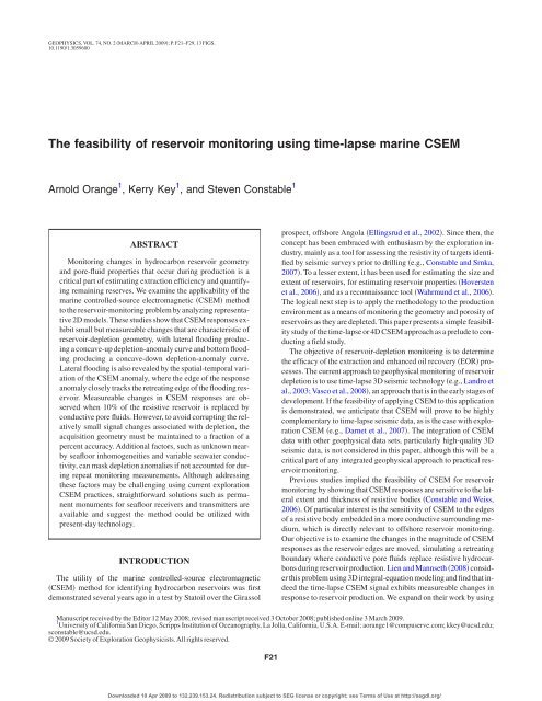
GEOPHYSICS, VOL. 74, NO. 2 MARCH-APRIL 2009; P. F21–F29, 13 FIGS.
10.1190/1.3059600
The feasibility of reservoir monitoring using time-lapse marine CSEM
Arnold Orange 1 , Kerry Key 1 , and Steven Constable 1
ABSTRACT
Monitoring changes in hydrocarbon reservoir geometry
and pore-fluid properties that occur during production is a
critical part of estimating extraction efficiency and quantifying
remaining reserves. We examine the applicability of the
marine controlled-source electromagnetic CSEM method
to the reservoir-monitoring problem by analyzing representative
2D models. These studies show that CSEM responses exhibit
small but measureable changes that are characteristic of
reservoir-depletion geometry, with lateral flooding producing
a concave-up depletion-anomaly curve and bottom flooding
producing a concave-down depletion-anomaly curve.
Lateral flooding is also revealed by the spatial-temporal variation
of the CSEM anomaly, where the edge of the response
anomaly closely tracks the retreating edge of the flooding reservoir.
Measureable changes in CSEM responses are observed
when 10% of the resistive reservoir is replaced by
conductive pore fluids. However, to avoid corrupting the relatively
small signal changes associated with depletion, the
acquisition geometry must be maintained to a fraction of a
percent accuracy. Additional factors, such as unknown nearby
seafloor inhomogeneities and variable seawater conductivity,
can mask depletion anomalies if not accounted for during
repeat monitoring measurements. Although addressing
these factors may be challenging using current exploration
CSEM practices, straightforward solutions such as permanent
monuments for seafloor receivers and transmitters are
available and suggest the method could be utilized with
present-day technology.
INTRODUCTION
The utility of the marine controlled-source electromagnetic
CSEM method for identifying hydrocarbon reservoirs was first
demonstrated several years ago in a test by Statoil over the Girassol
prospect, offshore Angola Ellingsrud et al., 2002. Since then, the
concept has been embraced with enthusiasm by the exploration industry,
mainly as a tool for assessing the resistivity of targets identified
by seismic surveys prior to drilling e.g., Constable and Srnka,
2007. To a lesser extent, it has been used for estimating the size and
extent of reservoirs, for estimating reservoir properties Hoversten
et al., 2006, and as a reconnaissance tool Wahrmund et al., 2006.
The logical next step is to apply the methodology to the production
environment as a means of monitoring the geometry and porosity of
reservoirs as they are depleted. This paper presents a simple feasibility
study of the time-lapse or 4D CSEM approach as a prelude to conducting
a field study.
The objective of reservoir-depletion monitoring is to determine
the efficacy of the extraction and enhanced oil recovery EOR processes.
The current approach to geophysical monitoring of reservoir
depletion is to use time-lapse 3D seismic technology e.g., Landro et
al., 2003; Vasco et al., 2008, an approach that is in the early stages of
development. If the feasibility of applying CSEM to this application
is demonstrated, we anticipate that CSEM will prove to be highly
complementary to time-lapse seismic data, as is the case with exploration
CSEM e.g., Darnet et al., 2007. The integration of CSEM
data with other geophysical data sets, particularly high-quality 3D
seismic data, is not considered in this paper, although this will be a
critical part of any integrated geophysical approach to practical reservoir
monitoring.
Previous studies implied the feasibility of CSEM for reservoir
monitoring by showing that CSEM responses are sensitive to the lateral
extent and thickness of resistive bodies Constable and Weiss,
2006. Of particular interest is the sensitivity of CSEM to the edges
of a resistive body embedded in a more conductive surrounding medium,
which is directly relevant to offshore reservoir monitoring.
Our objective is to examine the changes in the magnitude of CSEM
responses as the reservoir edges are moved, simulating a retreating
boundary where conductive pore fluids replace resistive hydrocarbons
during reservoir production. Lien and Mannseth 2008 consider
this problem using 3D integral-equation modeling and find that indeed
the time-lapse CSEM signal exhibits measureable changes in
response to reservoir production. We expand on their work by using
Manuscript received by the Editor 12 May 2008; revised manuscript received 3 October 2008; published online 3 March 2009.
1 University of California San Diego, Scripps Institution of Oceanography, La Jolla, California, U.S.A. E-mail: aorange1@compuserve.com; kkey@ucsd.edu;
sconstable@ucsd.edu.
© 2009 Society of Exploration Geophysicists.All rights reserved.
F21
Downloaded 10 Apr 2009 to 132.239.153.24. Redistribution subject to SEG license or copyright; see Terms of Use at http://segdl.org/

F22
Orange et al.
accurate 2D finite-element modeling to study several variations of a
depleting reservoir, including lateral and bottom flooding, stacked
reservoirs, and partial-depletion effects. Because the total volume of
oil or gas extracted from a reservoir is a known quantity, CSEM must
be able to discriminate between such different depletion scenarios to
be useful. Additionally, we present several acquisition and environmental
factors that could confound time-lapse interpretations.
Reservoir-depletion monitoring is the primary force driving this
research, but there are other possible applications for offshore timelapse
CSEM monitoring, such as CO 2 sequestration, waste sites,
freshwater aquifers, seafloor volcanoes, hydrothermal vents, and
geothermal regions, which may exhibit time-varying conductivity
structure. Our studies also demonstrate the sensitivity of exploration
CSEM to the size and shape of 2D reservoirs.
Our paper is organized as follows: In the first section, we present
the modeling methodology and show how the CSEM responses for
2D depletion scenarios are characteristic of the flooding geometry.
We then study a few environmental and acquisition factors that
could confound the CSEM interpretation if not properly accounted
for. We conclude the paper with a discussion of practical considerations
for offshore CSEM monitoring and provide suggestions for
data acquisition protocols that can address the high levels of accuracy
and repeatability required.
2D RESERVOIR-DEPLETION STUDIES
In this section we present a 2D analysis of simplified models of
reservoir depletion. Previous studies consider the sensitivity to thin
a)
b)
Depth (km)
0
1.5
2.5
z
Not to scale
Canonical
Left flood
Bottom flood
x
y
Receiver
–-2 km
0
Sediments 1.0 ohm-m
5km
100 ohm-m
Transmitters
Reservoir 100 ohm-m
Flooded volume—
within dotted lines
50 m
100 m
Figure 1. a The 2D canonical model used for the simulations. The
single receiver is located at position 2 km, and the transmitters are
positioned 50 m above the seafloor and are spaced at 250-m intervals
from 4 to 15 km. The transmissions are computed at 0.1 Hz.
b The reservoir geometry for the canonical, left, and bottom flooding
models.
1D resistive structures and show that the inline CSEM response varies
almost linearly with reservoir thickness e.g., Figure 10 in Constable
and Weiss, 2006. Although 1D studies are useful for generating
basic CSEM insights, they are not applicable to monitoring problems
because the finite width of the reservoir is a critical parameter
in quantifying the nature of extraction.
More importantly, the 2D results we present for the model in Figure
1 demonstrate that the lateral edges of the reservoir impart a
strong signal in the CSEM responses Figure 2. Later, we show that
this signal varies substantially as the reservoir is depleted. The 2D
model responses in Figure 2 are qualitatively similar to the responses
for a 3D resistive disk shown in Constable and Weiss 2006, and
both 2D and 3D responses are significantly different from the 1D response
past the edges of the resistive body. Actual survey data may
require 3D tools, but we propose that 2D studies are a sufficient starting
point for generating insights on the time-lapse monitoring problem.
We expect that low percentage-depletion scenarios will only generate
small changes in the CSEM responses. To quantify these
changes accurately, we need to consider the accuracy of our numerical
modeling approach. Here, we use the MARE2DCSEM code
modeling with adaptively refined elements for 2D CSEM; Li and
Key, 2007, which uses an adaptive finite-element method to generate
arbitrarily accurate 2.5D CSEM responses. Although accurate
responses can be generated by manually creating a very densely
gridded finite-element mesh, MARE2DCSEM constructs a much
more efficient mesh by automatically performing adaptive mesh refinement
until the CSEM responses reach a user-specified accuracy.
The code accomplishes this by using a superconvergent gradient
recovery operator to estimate the solution error in each element of
the mesh. This error is then weighted by an adjoint solution of the
a)
Amplitude (log10 V/Am
2 )
b)
Amplitude (log10 V/Am 2 )
c)
Amplitude (log10 T/Am)
−6
−8
−10
−12
−14
1D canonical
2D canonical
1 ohm-m half-space
−16
−5 0 5 10 15
Transmitter position along y (km)
−8
−10
−12
−14
−16
−18
−5 0 5 10 15
Transmitter position along y (km)
−10
−12
−14
−16
−18
−20
−5 0 5 10 15
Transmitter position along y (km)
Phase lag (º)
Phase lag (º)
Phase lag (º)
0
50
100
150
200
250
−5 0 5 10 15
Transmitter position along y (km)
−200
0
200
400
600
800
−5 0 5 10 15
Transmitter position along y (km)
0
100
200
300
400
500
−5 0 5 10 15
Transmitter position along y (km)
Figure 2. CSEM responses for the 1D and 2D canonical models and a
1-ohm-m half-space are shown for a the inline electric field E y , b
vertical electric field E z , and c azimuthal magnetic field B x .
Downloaded 10 Apr 2009 to 132.239.153.24. Redistribution subject to SEG license or copyright; see Terms of Use at http://segdl.org/

Marine 4D CSEM reservoir monitoring
F23
2.5D differential equation, where the sourcing functions are the estimated
errors at the discrete EM receivers. The adjoint solution provides
an influence, or sensitivity, function for the global mesh errors.
Thus, only elements with errors that contribute to the solution error
at the discrete EM receivers are refined. Details of the adaptive refinement
method and a validation of the method’s accuracy for
CSEM modeling are given in Li and Key 2007. For the model simulations
presented here, we set the tolerance so that the finite-element
mesh was refined until the estimated relative error in the CSEM
responses was below 0.1%.
Base model
The base model for our simulations is the 2D canonical model,
shown in Figure 1a. This model is the 2D analog of the 1D canonical
reservoir model presented in Constable and Weiss 2006 and consists
of a 100-m-thick, 5-km-wide, 100-ohm-m reservoir buried
1000 m below the seafloor with an ocean depth of 1500 m. For the
monitoring simulations, we perturb the model by depleting flooding
the reservoir by raising the bottom surface bottom flood, Figure
1b or by moving the left edge inward left flood, Figure 1b over a
range of depletions that vary from 0–80%. We model the CSEM responses
for a single receiver located 2 km to the left of the reservoir
for a series of inline electric dipole transmitters spaced every 250 m
from 4 to 15 km horizontal position at 50 m above the seafloor.
The transmitter and receiver computations assume a point dipole approximation,
and all models are computed for 0.1-Hz transmissions.
Figure 2 shows the CSEM amplitude and phase responses for the
1D and 2D canonical models and a uniform half-space seafloor model.
As mentioned, the 2D responses differ substantially from the 1D
responses, and all field components show an inflection when the
transmitter is over the right edge of the reservoir. Figure 2 identifies
where the responses are larger than the noise floor of present-day
transmitter-receiver systems around 10 15 V/Am 2 for electric
fields and 10 18 T/Am for magnetic fields. For instance, the inline
electric field is above this noise floor where the transmitter is located
at positions less than 12 km i.e., up to 14 km source-receiver offset.
For the remainder of the model studies, we present the CSEM responses
as the ratio of the responses for the model with the reservoir
to that of the 1D half-space case, i.e., to the case without the reservoir.
The plots are thus of the relative anomaly caused by the presence
of the reservoir canonical, or perturbed by flooding in an otherwise
uniform 1-ohm-m half-space. The phase of the CSEM responses
clearly contains useful 2D structural information see Figure
2, yet for brevity we restrict most of our analysis here to studying
amplitude anomalies.
Lateral and bottom flooding
In Figure 3, we present an anomaly comparison for models of bottom
depletion with models of depletion laterally from the left. The
cases shown are for no flood 2D canonical model and for a flood
completely water-filled reservoir volume of 10%, 20%, 40%, 60%,
and 80%. The water-filled portion of the reservoir has the same resistivity
as the background half-space 1 ohm-m. Currently, the most
commonly collected data are the horizontal electric field, designated
E y for radial-mode 2D modeling Figure 3a. We also show the results
for the vertical electric field E z Figure 3b and the azimuthal
magnetic field B x Figure 3c. The results for each of the lateral-flood
and bottom-flood comparisons are plotted to the same scale for each
component.
Figure 3 shows that the reservoir-caused anomalies are strongest
when the transmitter is over the far edge of the reservoir near 5 km,
and this peak anomaly resides at this position even in the presence of
significant flooding. Thus, the distal edge of the reservoir seems to
be an ideal transmission location or, through Lorentz reciprocity, an
ideal receiving location for exploration and monitoring field surveys.
There is little anomalous response when the transmitter is over
the near edge 0 km because of the absence of resistive structure between
the source and receiver and the relatively shallow sensitivity
at short offsets. For lateral and bottom flooding, the strongest anomaly
is present in the azimuthal magnetic field; the weakest anomaly
still of considerable size is in the inline electric field. For lateral
flooding, the left edge of the anomalies moves in direct correspondence
with the flooded edge of the reservoir, suggesting that CSEM
monitoring may be able to distinguish which sides of the reservoir
retreat during production.
Figure 4 shows the anomaly strength at 5 km as a function of
flooding percentage. The anomaly magnitudes shrink as flooding increases,
but the behavior of this decrease differs for the two flooding
types. For all three components, flooding from the left results in a
large decrease in anomaly amplitude during the early stages of depletion,
which then slows down in the later stages, giving a concaveup
depletion-anomaly curve. The opposite is seen for the basal
a)
Anomaly (ratio)
b)
Anomaly (ratio)
c)
Anomaly (ratio)
3.5
3
2..5
2
1.5
1
0.5
Flood from left
% Flood:
0
10
20
40
60
80
0
−4 −2 0 2 4 6 8 10 12 14 16
0
−4 −2 0 2 4 6 8 10 12 14 16
7
6
5
4
3
2
1
7
6
5
4
3
2
1
0
−4 −2 0 2 4 6 8 10 12 14 16
Transmitter position (km)
3..5
3
2.5
2
1.5
1
0.5
Flood from bottom
% Flood:
0
10
20
40
60
80
0
−4 −2 0 2 4 6 8 10 12 14 16
7
6
5
4
3
2
1
0
−4 −2 0 2 4 6 8 10 12 14 16
7
6
5
4
3
2
1
0
−4 −2 0 2 4 6 8 10 12 14 16
Transmitter position (km)
Figure 3. Depletion simulations for left flooding left column and
bottom flooding right column. The a inline electric field E y , b
vertical electric field E z , and c azimuthal magnetic field B x amplitude
anomalies are shown as the ratio of the 2D to half-space responses.
Percent flood refers to the percent volume replaced by
1-ohm-m material, identical to the background resistivity.
Downloaded 10 Apr 2009 to 132.239.153.24. Redistribution subject to SEG license or copyright; see Terms of Use at http://segdl.org/

F24
Orange et al.
flooding, where the early stages of flooding produce only small
anomaly changes but late stages of flooding give a significant anomaly
decrease, resulting in a concave-down depletion-anomaly curve.
This systematic behavior may be a simple and useful tool for distinguishing
between flooding types, although whether this holds for
more complicated reservoirs remains to be studied. A corollary of
the interpretation of Figure 3 that applies to exploration CSEM is
that thin and wide reservoirs produce larger CSEM responses than
thick and narrow reservoirs.
There are other subtleties associated with evaluating reservoir-depletion
characteristics using CSEM. Consider the two sets of curves
for the radial electric field E y in Figure 3a. The response for a 40%
bottom flood is very similar to that for a 10% lateral flood. Likewise,
the 80% bottom flood has an anomaly similar to the 40% lateral flood
case. If the original reservoir volume is known, then the total production
volume could be used to discriminate between left and bottom
flooding models in these examples. The curve shapes for these reservoir
geometries differ and provide a modicum of diagnostic evidence
for determining where flooding occurs. The same observations
could be made for the other field components.
a)
Anomaly (ratio)
b)
Anomaly (ratio)
c)
Anomaly (ratio)
3
2.5
2
1.5
1
0 10 20 30 40 50 60 70 80 90 100
Percent flood
6
5
4
3
2
1
0 10 20 30 40 50 60 70 80 90 100
Percent flood
7
6
5
4
3
2
Left flood
Bottom flood
Left flood
Bottom flood
Left flood
Bottom flood
1
0 10 20 30 40 50 60 70 80 90 100
Percent flood
Figure 4. Anomaly strength as a function of percent depletion for
when the transmitter is located over the right edge of the reservoir
5 km. The a inline electric field E y , b vertical electric field E z ,
and c azimuthal magnetic field B x are shown for left and bottom
flooding.
Effect of water depth
We also computed responses for the flooded reservoir models at a
different water depth to study the effect of the airwave, a term used to
describe energy that propagates along the air-sea interface. At short
offsets, the fields measured by the receivers predominantly diffuse
through the ocean and seabed; at longer offsets, the fields result from
a combination of the airwave and diffusion through the reservoir and
seabed Constable and Weiss, 2006. The fields observed on the seafloor
are the result of constructive or destructive interference between
the airwave and reservoir wave, as determined by their respective
amplitudes, phases, and vector orientations.
Because the airwave experiences complex attenuation as it diffuses
from the transmitter up to the sea surface and later back down to
the seafloor, the long-offset fields observed on the seafloor vary substantially
with ocean depth. See also Weidelt 2007 for a theoretical
analysis of EM waves guided in the resistive air and reservoir
layers. In the example that follows, we demonstrate how the airwave’s
dependence on the ocean depth can affect the magnitude of
CSEM anomalies significantly.
Figure 5 shows the anomaly responses for the lateral flooding case
for ocean depths of 1500 and 3000 m and flooding of 0%, 10%, and
20%, with all other parameters as in Figure 3. The plots on Figure 5
use the same vertical scale for each component, emphasizing the
large variations in the size of the reservoir-induced anomaly with
ocean depth. This variation is inconsistent among the three field
a)
Anomaly (ratio)
b)
Anomaly (ratio)
c)
Anomaly (ratio)
7
6
5
4
3
2
1
Water depth 1500 m
% Flood:
0
10
20
0
−4 −2 0 2 4 6 8 10 12 14 16
0
−4 −2 0 2 4 6 8 10 12 14 16
7
6
5
4
3
2
1
7
6
5
4
3
2
1
0
−4 −2 0 2 4 6 8 10 12 14 16
Transmitter position (km)
7
6
5
4
3
2
1
Water depth 3000 m
% Flood:
0
10
20
0
−4 −2 0 2 4 6 8 10 12 14 16
7
6
5
4
3
2
1
0
−4 −2 0 2 4 6 8 10 12 14 16
7
6
5
4
3
2
1
0
−4 −2 0 2 4 6 8 10 12 14 16
Transmitter position (km)
Figure 5. The effect of ocean depth on the anomaly amplitudes. a
Inline electric field E y , b vertical electric field E z , and c azimuthal
magnetic field B x anomalies associated with the perturbations of the
2D canonical model for two water depths: 1500 m left column and
3000 m right column.
Downloaded 10 Apr 2009 to 132.239.153.24. Redistribution subject to SEG license or copyright; see Terms of Use at http://segdl.org/

Marine 4D CSEM reservoir monitoring
F25
components. For E y Figure 5a, the anomaly at 3000 m ocean depth
is about double that at 1500 m; the reverse is true for B x Figure 5c.
Other changes appear at positions greater than 8 km, where E y for a
3000-m ocean depth has a second anomaly peak at about 14 km and
B x has a second peak at about 11 km. Clearly, these second peaks are
related to the ocean depth, showing that the airwave is strongly coupled
to the sea layer because the anomaly varies with ocean depth
and coupled with the wave traveling up from the reservoir because
an anomaly is present.
Although not shown here, systematic variation of the ocean depth
from 1500 to 3000 m shows that these second anomaly peaks move
to increasingly farther distances as water depth increases. We conclude
that for a 1500-m ocean depth, the airwave-influenced response
begins near the middle of the reservoir, but for a 3000-m
ocean depth, the airwave does not affect the responses until a few kilometers
past the edge of the reservoir.
The ability to detect the flood with the horizontal components appears
not to be affected in either case because the relative changes
between flood-induced anomalies is nearly constant in the vicinity
of the reservoir. As anticipated, the vertical electric field E z , Figure
5b is influenced least by the changes in the water depth.
Stacked reservoirs
The canonical reservoir Figure 1a is clearly an oversimplification
of most real-world reservoirs. Figure 6a depicts a somewhat
a)
166.6 ohm-m
1 ohm-m
166.6 ohm-m
1 ohm-m
166.6 ohm-m
5000 m
20 m
20 m
20m
20 m
20 m
100 m
more complex scenario: a three-layer reservoir sequence where the
total vertical resistance layer thickness times layer resistivity of the
three layers is equivalent to that of the single-layer canonical model.
The three 20-m-thick, 166.6-ohm-m layers with 20-m-thick, 1-ohm
-m intervals between the layers span the same 100-m total thickness
of the canonical model. Although not shown here, the responses for
this model differ from the canonical 2D model shown in Figure 1a by
less than 0.5% for all three components — that is, this layered reservoir
has nearly the same response as the 2D canonical reservoir. This
unsurprising result suggests that CSEM will be limited in the ability
to resolve closely spaced reservoir units, and to do so will require
some significant a priori structural constraints.
We modeled a 20% depletion of the center of the three layers Figure
6b to evaluate the results of a more subtle depletion scenario.
This corresponds to a 7% flood of the complete three-layer reservoir.
Figure 7 shows the ratio of the CSEM response of the three-layer unflooded
model to that of the model with a 20% flood of the center lay-
a)
Anomaly (ratio)
b)
1.05
1.04
1.03
1.02
1.01
1
0.99
0.98
−5 0 5 10 15
−3.5
−3
Bx
Ey
Ez
Ey
Ez
Bx
−2.5
b)
Flood
1000 m
Phase difference (º)
−2
−1.5
−1
−0.5
0
0.5
Figure 6. a Multilayer anisotropic reservoir model with a total
vertical resistance of the combined three layers identical to the canonical
model shown in Figure 1a. bA20% flood of the middle layer
of the model in a.
1
−5 0 5 10 15
Transmitter position along y (km)
Figure 7. a Anomaly ratio and b phase difference for the threelayer
reservoir model without flood Figure 6a compared to the
three-layer model with 20% flood of the middle layer Figure 6b.
Downloaded 10 Apr 2009 to 132.239.153.24. Redistribution subject to SEG license or copyright; see Terms of Use at http://segdl.org/

F26
Orange et al.
er. The maximum anomaly is on the order of 2–4%, with the largest
anomaly on the B x component. For each component, the anomaly
onset occurs at or near the left edge of the reservoir assembly, coincident
with flooding from the left.
Partial-depletion effects
Given current extraction efficiencies, it is likely that a significant
residue of hydrocarbons will remain in the flooded section of the reservoir,
and it is important to consider the impact this may have on
time-lapse CSEM. Consider the case where the production engineer
states that 20% volume of the reservoir has been extracted. Figure 8
shows five variations of left flooding for this scenario, where the
width of the flooded section depends on the fraction of hydrocarbons
remaining in place. ModelAis for complete extraction 100% depletion,
as used for the previous studies shown here. Models B-E show
a varying percentage of depletion in the flooded section 80–20%.
The resistivity of the partially depleted section is computed as a
function of the pore space occupied by water using Archie’s law:
f d 2 , where the water resistivity f 0.16 ohm-m, the porosity
40%, and d is the reservoir-depletion factor.
Figure 9 shows the CSEM anomalies for these scenarios. ModelA
100% depletion shows the largest anomaly; model D 40% depletion
shows the weakest anomaly. These end members’ anomalies
are about 10% different for the E y component and 30% different for
the E z and B x components. Models A-D all have relatively low resistivity
in the flooded section; hence, the anomalies correlate largely
with the size of the unflooded reservoir section. Model E reverses the
decreasing anomaly trend and exhibits a larger anomaly than model
D. However, this is easily explained because model E has more remaining
oil in place in the flooded section i.e., the entire reservoir
and hence has a much higher resistivity than model D.
The difference in anomalies between any of these models is at
least a few percent, suggesting that exploration or time-lapse CSEM
could be used to discriminate between varying degrees of reservoir
Depletion
A: 100% 1 ohm-m
B:
1km
80% 1.6 ohm-m
C: 60%
D: 40%
E: 20%
5 km
100 ohm-m
4km
100 ohm-m
1.25 km 3.75 km
2.8 ohm-m
100 ohm-m
1.67 km 3.33 km
6.2 ohm-m
100 ohm-m
2.5 km 2.5 km
25 ohm-m
5 km
Figure 8. Five reservoir models representing 20% recovery of the
original reservoir volume caused by flooding from the left. Models
A–E show decreasing levels of depletion in the flooded region.
100 m
saturation. Furthermore, there is at least a 25% difference in anomaly
size between any of these models and the 0% extraction i.e., 0%
flooded models shown in the left column of Figure 3, indicating that
all of these scenarios produce measureable time-lapse signals.
We have presented variations for only a few model parameters;
clearly, this work could be expanded to study the effects of frequency,
depth of reservoir burial, reservoir thickness, variable background
resistivity, resistivity contrasts, and the multiple receiver locations
typical of CSEM field surveys. However, the results presented
here are representative based on many other 2D computations we
have made.
a)
Anomaly (ratio)
2
1.8
1.6
1.4
1.2
1
b) 4
Anomaly (ratio)
c)
Anomaly (ratio)
A
B
C
D
E
0.8
−5 0 5 10 15
3.5
3
2.5
2
1.5
1
0.5
−5 0 5 10 15
4.5
4
3.5
3
2.5
2
1.5
1
0.5
−5 0 5 10 15
Transmitter position along y (km)
Figure 9. Anomaly ratios for the five partial-depletion models shown
in Figure 8.Anomalies are computed by normalizing by a half-space
response. The a inline electric field E y , b vertical electric field E z ,
and c azimuthal magnetic field B x .
Downloaded 10 Apr 2009 to 132.239.153.24. Redistribution subject to SEG license or copyright; see Terms of Use at http://segdl.org/

Marine 4D CSEM reservoir monitoring
F27
FACTORS AFFECTING CSEM RELIABILITY
It is clear from the model studies that for time-lapse CSEM to succeed,
measurement repeatability must be better than 5% — possibly
better than 1–2% — to characterize the flooding geometry. Obviously,
it will not be good enough to state that the reservoir is shrinking
because the production manager knows that from the production
rates. The subtle changes expected in reservoir geometry as the reservoir
is depleted will require the ability to measure equally subtle
changes in the CSEM response. In this section we present some examples
of factors that could affect CSEM reliability — notably, the
repeatability and accuracy required for time-lapse interpretation.
These factors affect exploration use of CSEM as well for those cases
where the expected anomalies are only slightly larger than the system
noise floor and navigation uncertainties.
Effect of near-surface inhomogeneities
The near-surface environment should not be expected to be homogeneous
in every case. For example, Weitemeyer et al. 2006 use
CSEM field data to constrain significant shallow resistivity variations
associated with methane hydrates and free gas. Other studies
consider how shallow structures can create significant CSEM anomalies
e.g., Darnet et al., 2007. Here, we present an example that
demonstrates that a small near-surface resistive body can produce
anomalies of size comparable to those of a depleting reservoir.
The model is shown in Figure 10a and includes the standard 2D
canonical reservoir Figure 1a but with a 10-m-thick, 100-m-wide,
5-ohm-m body placed on the seafloor 2 km from the left edge of the
reservoir. We computed the CSEM responses for a series of receivers
placed on and adjacent to the body, as shown in
Figure 10a. Site A is over the center of the body,
site B is on the body 25 m inward from the right
edge, and sites C, D, and E are 25, 50, and 100 m
away from the right edge of the body, respectively.
The CSEM anomalies are presented in Figure
10b-d and show the response ratios of this model
to the model without the near-surface resistor.
The impact of the near-surface feature is significant
and varies with component. The maximum
effect in all components occurs when the
source is located over the resistive body, in agreement
with a previous study of 3D Fréchet derivatives
that illustrated a strong sensitivity to seawater
and seafloor conductivity in the region immediately
surrounding the transmitter Weiss and
Constable, 2006. When the source is away from
the body, a 40–50% anomaly is observed in the
vertical electric field Figure 10c for the two sites
located over the body, sites A and B. Site C, the
first site off of the body, exhibits an approximately
7% effect. The effect on the radial electric field
Figure 10b is less and reaches a maximum of
8–12% for the sites that straddle the boundary of
the near-surface body. The least effect 5% is
for the azimuthal magnetic field Figure 10d.
Note that the effect observed in Figure 10b and
c extends over a broad range of transmitter-receiver
separations and could confound an interpretation,
especially if such shallow bodies were
a)
Depth (km)
b)
Anomaly (ratio)
1.48
1.49
1.5
1.51
1.2
1.15
1.1
1.05
1
0.95
0.9
10 m
common within the survey area. This is a principal argument for precise
placement of receivers for repeat reservoir monitoring measurements
because imprecise receiver replacement near a feature like
this could lead to false reservoir-depletion anomalies. This is also an
important consideration in exploration surveys in areas where nearsurface
inhomogeneities such as hydrates are suspected. Although
not shown here, we have modeled the analogous scenario where an
isolated shallow body is below the transmitter and is located several
kilometers from the receivers.As anticipated, the anomaly produced
by this feature is confined to data collected only when the transmitter
is located over the body.
Effect of ocean conductivity
In Figure 11, we investigate the effect of seawater resistivity,
which changes over time because of salinity and thermal variations
associated with ocean currents and river outflows. We examine the
variation in response when seawater resistivity changes from the
0.330-ohm-m value used in the previous models to a new value of
0.315 ohm-m a 4.5% difference.
The results in Figure 11 show a variation in response of up to 10%
in amplitude and a few degrees in phase. The strongest change is in
the E y and B x components and occurs when the influence of the airwave
is strongest, at transmitter-receiver offsets of 10 km and greater.
This is explained because the airwave must travel through the entire
water column and the attenuation of the signal within the seawater
is strongly a function of conductivity. If time-lapse survey data
were compared without accounting for a change in seawater resistivity,
a false depletion anomaly might result.
B
A
0.33 ohm-m
Sites: A B C D E
5 ohm-m 1 ohm-m
100 m
Edge of reservoir
1.52
−2.1 −2.05 −2.0 −1.95 −1.90 −1.85
Position (km)
0.85
−5 0 5 10 15
Transmitter position (km)
D
Receivers
E
C
c)
Anomaly (ratio)
d)
Anomaly (ratio)
2.2
2
1.8
1.6
1.4
1.2
1
0.8
0.6
−5 0 5 10 15
Transmitter position (km)
1.2
1.15
1.1
1.05
1
0.95
0.9
A
C
Receivers
0.85
−5 0 5 10 15
Transmitter position (km)
Figure 10. The effect of a seafloor inhomogeneity. Ratio of CSEM response of the 2D canonical
model without seafloor inhomogeneity to that with the seafloor inhomogeneity.
a Receiver locations, b inline electric field E y , c vertical electric field E z , and d azimuthal
magnetic field B x .
B
D
Downloaded 10 Apr 2009 to 132.239.153.24. Redistribution subject to SEG license or copyright; see Terms of Use at http://segdl.org/

F28
Orange et al.
A precise analysis of CSEM results thus requires precise knowledge
of the characteristics of the seawater. This should not be a problem
because the commonly used conductivity-temperature-depth
CTD probes accurately measure the seawater properties. However,
interpretation and modeling for the level of accuracy required for
time-lapse CSEM requires that these data be acquired at the time
CSEM data are recorded. Because seawater temperature variations
are strongest in the upper few hundred meters of the water column,
this problem is most severe for shallow-water applications.
Errors in transmitter geometry and receiver locations
Given adverse weather conditions and strong ocean currents, the
transmitter antenna vector often can be rotated from ideal survey
specifications. In Figure 12, we investigate the effects of transmitter
dipole pitch variations of 10° up and down, where we plot the ratio of
the response for the dipping dipole to a purely horizontal dipole. The
false anomalies this produces vary spatially and are greatest when
the transmitter is near the receivers. When the transmitter is more
than a few kilometers away, both the 10° dip-down Figure 12a 10°
dip-up Figure 12b transmitters result in a somewhat smaller variation
in response of about 15–20%. For the case of a dipole yaw and
the symmetric model considered here, the perturbation is described
by a cosine yaw angle scaling. These effects must be taken into account,
because they are equal to or greater than the effects observed
from reservoir flooding. We have modeled a dipping point dipole,
whereas dip in the finite-length bipoles used in field surveys results
in one electrode being closer to the seafloor, so the effect of dip will
probably be greater than is shown here.
Last, we investigate the effect of an error in the lateral location of
the receiver or transmitter. Figure 13 shows the response variation
as we move the receiver 25 and 50 m from its correct position.
Again, the false anomaly this produces is largest when the transmitter
is over the receiver. When the transmitter is at least a few kilometers
away, a 50-m lateral position error Figure 13b results in a false
anomaly of about 5%; a 25-m position error Figure 13a yields a
smaller, approximately 2% anomaly. These false anomalies extend
well to the right of the reservoir boundary. Extrapolation of these results
suggests that seafloor receiver positions should be known and
repeatable to less than 5–10 m accuracy to detect time-lapse depletion
anomalies.
Figure 11. Effect of seawater conductivity variations on CSEM a
anomaly ratio and b phase difference. Ratio of 2D canonical response
with 0.33-ohm-m seawater to that with 0.315-ohm-m seawater
a 4.5% difference.
Figure 12. Effect of transmitter dipole dip. Ratio of 2D canonical response
with transmitter dipole dipping to that with a horizontal dipole:
a dip 10° down; b dip 10° up.
Downloaded 10 Apr 2009 to 132.239.153.24. Redistribution subject to SEG license or copyright; see Terms of Use at http://segdl.org/

Marine 4D CSEM reservoir monitoring
F29
a)
Anomaly (ratio)
b)
Anomaly (ratio)
1.15
1.1
1.05
1
0.95
0.9
−5 0 5 10 15
1.15
1.1
1.05
1
0.95
CONCLUSIONS
Ey
Ez
B x
Ey
Ez
B x
0.9
−5 0 5 10 15
Transmitter position along y (km)
Receiver
Figure 13. Effect of error in receiver location. Ratio of response with
receiver at 2 km to response with receiver at a 25 m and b
50 m to the left.
We have shown through a series of 2D model studies that a depleting
reservoir can produce small but measureable changes in CSEM
response over time, and these changes can be characteristic of the depletion
geometry. It is understood that 3D analysis of more complex
and realistic reservoir scenarios will be required to provide guidance
for practical applications. However, our studies suggest that being
able to provide useful information on reservoir geometry and resistivity
to the reservoir engineer during production will require the
ability to resolve changes in the CSEM response over time of at best
a few percent. This in turn will require repeatability of the basic
CSEM measurement to 1%–2% or better. This is probably not possible
using the current technology of free-falling receivers, towed
transmitters, and supershort baseline positioning technology, especially
in deepwater areas.
There are several possible solutions, and the CSEM industry will
be challenged to find those that provide the required accuracy yet remain
cost effective. Obviously, permanent installation of EM receivers
and transmitters on the seafloor would be an attractive alternative,
but this is likely to be impractical. Permanent monuments to
which receivers and transmitters could be affixed by remotely operated
vehicles is an attractive approach because the position repeatability
could be on the order of 1 m or less. This approach mitigates
the effect of unknown seafloor inhomogeneities as well as the often
large uncertainties in position, altitude, dip, and yaw of a deep-towed
source antenna.Accurate characterization of the electrical properties
of the water column is possible through the use of CTD instrumentation,
routinely used by oceanographers worldwide.
Yet another factor to consider for the repeatability of CSEM measurements
is changes to oilfield infrastructure — the pipelines, cables,
steel templates, etc., installed on the seafloor during the life of a
producing reservoir. Given their limited spatial extent, it may be possible
to plan time-lapse measurements so that source-receiver paths
largely avoid such structures, but certainly there will be survey geometries
where crossing infrastructure is unavoidable. Steel casings
and other conductive infrastructure have much smaller skin depths
than seawater and sediments and may distort the CSEM transmissions
locally. Such distortions are probably confined to where the
transmitter or receivers are located close to infrastructure, but careful
modeling and analysis will be required to demonstrate this point.
In summary, time-lapse CSEM is likely to be a most demanding
application of EM geophysics, but there is nothing that we have examined
so far that implies it is impossible.
ACKNOWLEDGMENTS
This work was carried out under support from the Seafloor Electromagnetic
Methods Consortium at Scripps Institution of Oceanography.
Three reviewers provided helpful comments.
REFERENCES
Constable, S., and L. J. Srnka, 2007, An introduction to marine controlledsource
electromagnetic methods for hydrocarbon exploration: Geophysics
72, no. 2, WA3–WA12.
Constable, S., and C. J. Weiss, 2006, Mapping thin resistors and hydrocarbons
with marine EM methods: Insights from 1D modeling: Geophysics
71, no. 2, G43–G51.
Darnet, M., M. C. K. Choo, R.-E. Plessix, M. L. Rosenquist, K. Yip-Cheong,
E. Sims, and J. W. K. Voon, 2007, Detecting hydrocarbon reservoirs from
CSEM data in complex settings: Application to deepwater Sabah, Malaysia:
Geophysics 72, no. 2, WA97–WA103.
Ellingsrud, S., T. Eidesmo, S. Johansen, M. Sinha, L. MacGregor, and S.
Constable, 2002, Remote sensing of hydrocarbon layers by seabed logging
SBL: Results from a cruise offshoreAngola: The Leading Edge, 21,
972–982.
Hoversten, G. M., F. Cassassuce, E. Gasperikova, G. A. Newman, J. Chen, Y.
Rubin, Z. Hou, and D. Vasco, 2006, Direct reservoir parameter estimation
using joint inversion of marine seismic AVA and CSEM data: Geophysics,
71, no. 3, C1–C13.
Landro, M., H. H. Veire, K. Duffaut, and N. Najjar, 2003, Discrimination between
pressure and fluid saturation changes from marine multicomponent
time-lapse seismic data: Geophysics, 68, 1592–1599.
Li, Y., and K. Key, 2007, 2D marine controlled-source electromagnetic modeling:
Part 1 — An adaptive finite element algorithm: Geophysics, 72,no.
2, WA51–WA62.
Lien, M., and T. Mannseth, 2008, Sensitivity study of marine CSEM data for
reservoir production monitoring: Geophysics, 73, no. 4, F151–F163.
Vasco, D. W., H. Keers, J. Khazanehdari, and A. Cooke, 2008, Seismic imaging
of reservoir flow properties: Resolving water influx and reservoir permeability:
Geophysics, 73, no. 1, O1–O13.
Wahrmund, L. A., K. E. Green, D. Pavlov, and B. A. Gregory, 2006, Rapid
interpretation of CSEM reconnaissance data: 76th Annual International
Meeting, SEG, ExpandedAbstracts, 709–713.
Weidelt, P., 2007, Guided waves in marine CSEM: Geophysical Journal International,
171, 153–176.
Weiss, C. J., and S. Constable, 2006, Mapping thin resistors in the marine environment,
Part II: Modeling and analysis in 3D: Geophysics, 71, no. 6,
G321–G332.
Weitemeyer, K., S. Constable, K. Key, and J. Behrens, 2006, First results
from a marine controlled-source electromagnetic survey to detect gas hydrates
offshore Oregon: Geophysical Research Letters, 33, L03304.
Downloaded 10 Apr 2009 to 132.239.153.24. Redistribution subject to SEG license or copyright; see Terms of Use at http://segdl.org/