HYDRAULIC MODEL OF TRICKLE-IRRIGATION LATERALS - IWRA

HYDRAULIC MODEL OF TRICKLE-IRRIGATION LATERALS
Nina Philipova
Institute of Mechanics, Bulgarian Academy of Sciences,
Acad. G. Bonchev Str., Bl.4, Sofia 113, Bulgaria,
e-mail:philipova@imbm.bas.bg
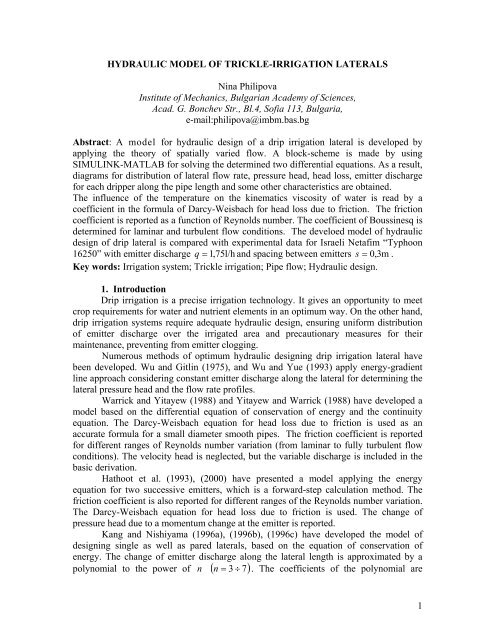
Abstract: A model for hydraulic design of a drip irrigation lateral is developed by
applying the theory of spatially varied flow. A block-scheme is made by using
SIMULINK-MATLAB for solving the determined two differential equations. As a result,
diagrams for distribution of lateral flow rate, pressure head, head loss, emitter discharge
for each dripper along the pipe length and some other characteristics are obtained.
The influence of the temperature on the kinematics viscosity of water is read by a
coefficient in the formula of Darcy-Weisbach for head loss due to friction. The friction
coefficient is reported as a function of Reynolds number. The coefficient of Boussinesq is
determined for laminar and turbulent flow conditions. The develoed model of hydraulic
design of drip lateral is compared with experimental data for Israeli Netafim “Typhoon
16250” with emitter discharge q = 1,75l/h
and spacing between emitters s = 0,3m .
Key words: Irrigation system; Trickle irrigation; Pipe flow; Hydraulic design.
1. Introduction
Drip irrigation is a precise irrigation technology. It gives an opportunity to meet
crop requirements for water and nutrient elements in an optimum way. On the other hand,
drip irrigation systems require adequate hydraulic design, ensuring uniform distribution
of emitter discharge over the irrigated area and precautionary measures for their
maintenance, preventing from emitter clogging.
Numerous methods of optimum hydraulic designing drip irrigation lateral have
been developed. Wu and Gitlin (1975), and Wu and Yue (1993) apply energy-gradient
line approach considering constant emitter discharge along the lateral for determining the
lateral pressure head and the flow rate profiles.
Warrick and Yitayew (1988) and Yitayew and Warrick (1988) have developed a
model based on the differential equation of conservation of energy and the continuity
equation. The Darcy-Weisbach equation for head loss due to friction is used as an
accurate formula for a small diameter smooth pipes. The friction coefficient is reported
for different ranges of Reynolds number variation (from laminar to fully turbulent flow
conditions). The velocity head is neglected, but the variable discharge is included in the
basic derivation.
Hathoot et al. (1993), (2000) have presented a model applying the energy
equation for two successive emitters, which is a forward-step calculation method. The
friction coefficient is also reported for different ranges of the Reynolds number variation.
The Darcy-Weisbach equation for head loss due to friction is used. The change of
pressure head due to a momentum change at the emitter is reported.
Kang and Nishiyama (1996a), (1996b), (1996c) have developed the model of
designing single as well as pared laterals, based on the equation of conservation of
energy. The change of emitter discharge along the lateral length is approximated by a
n = 3 ÷ 7 . The coefficients of the polynomial are
polynomial to the power of n ( )
1

determined using the least square method at a given inlet flow rate of lateral and at an
inlet pressure head of lateral. The Darcy-Weisbach equation for head loss due to friction
is used too. The friction coefficient is considered as a function of Reynolds number for
different flow conditions (from laminar to fully turbulent).
Kosturkov and Simeonov (1990), have developed a model of designing
horizontal, non- deformable trickle lateral on the basis of the momentum approach. The
longitudinal projection of discharged velocity is considered as a linear function of the
averaged flow velocity. An analytical decision of the two differential equations obtained
is proposed (the momentum equation and the conservation of mass equation) (Kosturkov,
1990).
Yildirim and Agiralioglu (2004) have performed a good comparative analysis of
the developed hydraulic methods in design of microirrigation laterals.
Von Bernurth (1990), Holzapfel et al. (1990), Bagarello et al. (1995) take into
account the influence of temperature on the viscosity change in the hydraulic design of
drip irrigation system. It is proved that when the water temperature changes from 15,5º C
to 37,7º C (from 60º F to 100º F) the density decreases by less than 1% but viscosity
decreases by about 40% (Munson, Young and Okishi, 1990). That is why the influence of
temperature and Reynolds number will be taken into account when the change of water
kinematic viscosity is considered.
The objective of the work presented in this paper is a model derivation for
hydraulic design of a drip lateral on the basis of theory of spatially varied flow and with
application in the drip irrigation practice.
2. Theoretical backgrounds of the developed model of trickle irrigation
laterals
The deduced model by Petrov (1951) is an one-dimensional hydraulic equation,
based on the momentum approach. It describes a steady spatially varied flow with
dz
averaged velocities, and inconstant flow area at slope with a gradient . The head loss
dx
due to friction is calculated by means of the formula of Darsy-Weisbach that is accurate
for a small diameter smooth pipes. The pipe is considered as non-deformable one. In the
case of lateral outflow along the pipe with a constant diameter, the equation is as follows:
2
1 dp dV dz V 1 ( V −θ
) V dQ
+ α V + + λ + α
= 0 , (1)
ρ dx dx dx 2 D Q dx
where: V is the averaged flow velocity throughout the cross-section; p is the pressure
assumed to be constant throughout the cross-section; α is a coefficient of Boussinesq; θ
is the longitudinal projection of discharged velocity , θ = δV
; δ is a coefficient of
proportionality between the longitudinal projection of discharged velocity and the
3
averaged flow velocity throughout the cross-section; Q is the flow rate in m / s ; γ is the
specific weight of water, γ = ρ g (for incompressible fluid); g - gravity acceleration.
The last term of the equation (1) reports discharging the flow along the lateral
length according to the theory of Meshterski (Petrov, 1951) and the previous term
represents the head loss due to the friction per unit length.
Taking into account the outflow at a distance between emitters s , the equation of
the conservation of mass is as follows:
2

dQ
dx
q
k
h
s
k 1
= − = − , (2)
where: q is the discharged flow per unit length in l / h (emitter outflow per unit length);
k
kh 1
is the exponential relationship of the dripper; k , k1
are constants depending on the
type of the dripper and its flow regime; h is the pressure head; s is the distance between
drippers.
3
Expressing the discharged flow per unit length q in m / s , the equation (2) obtains the
following form:
dQ
k k
= −q
= −F
1
Q
h , (3)
dx
s
where: is the coefficient converting from liters per hour to cubic meters per second,
F Q
F Q
= 2,7777x 10
-7
.
3. Formulas used for deriving model equation
The following basic equations are used:
3. The normal projection of friction forces for a lightly changed flow are neglected and
the pressure is constant throughout the cross-section. The pressure is as follows:
p = ρgh . (4)
2) The formulae for the ground slope:
dz
sin ψ = − , (6)
dx
where: ψ is the lateral slope angle;
3) The Darsy-Weisbach formulae for head loss which is due to friction per unit length
can be expressed as:
∆h
f
n m n
= K
loc
K
0FQ
D Q , (7)
l
∆h f
where: is the head loss due to the friction per unit length; n is the exponent of the
l
flow rate; m is the exponent of the pipe diameter; D is the pipe diameter, K
loc
is the
Benami and Offen coefficient (Benami and Offen, 1984) of the local head loss of
emitters, read as a function of the dripper type (online or inline), the distance between the
drippers and the pipe diameter; K 0
is the coefficient reading the kinematic viscosity
change as a function of temperature and Reynolds number.
4. The derived equation of the model
The following equation is derived on the basis of aforementioned equations (4) –
(7), the momentum equation of Petrov (1), and the equation of conservation of mass (3)
for steady flow movement with lateral outflow along the lateral length, where the crosssection
of the pipeline is assumed to be constant:
3

dh 1,6α
Q k1 n m n
g − g sinψ − kh ( 2 − δ ) + K
0
= 0,
4
loc
K FQ
D Q
(8)
dx
D
The other form of the derived model equation is the following:
dh 1,6α
Q
⎛ ∆h
k
f ∆h
⎞
1
loc
g − g sinψ − [ kh (2 − δ ] +
= 0
4 ⎜ +
⎟g
(9)
dx
D s
⎝ l l ⎠
where: ∆h loc
are the local head loss due to the emitters. Using this equation the formula
of Provenzano and Pumo (2003) can be used for estimating local head loss of “in-line”
drippers. Comperative analysis between the two approaches of local head loss estimating
for “in-line” emitters is performed in Philipova (2007a). The formula of Y. Reddy (2003)
could be used for estimating local head losses “on-line” emitters. Comperative analysis
between the two approaches of local head loss estimating for “in-line” emitters is
performed in Philipova (2007b)
Boundary conditions of the model are the following:
x = 0 Q = Q = Nq h = h ,
0
0
dQ
x = l = −q k
dx
where: Q is the inlet flow rate of the lateral; N is the number of emitters; q is the
0
nominal emitter discharge; h0
is the inlet pressure head; l is the length of the lateral,
is the last emitter discharge of the dripline
5. Head loss estimation due to friction
The head loss due to friction is a function of the Reynolds number (Warrick and
Yitayew, 1988, Hathoot et al.,1993, Kang and Nishiyama, 1996a).
1) The friction coefficient λ for laminar flow Re ≤ 2000 , is defined below:
64
λ = ,
Re
∆h
−4
−4
= 40,745ν Q D = K
0
Q D ,
l
(10)
K = 40,745ν 0 (10’)
where:ν is the kinematic viscosity of water.
n = 1;
m = −4 . (10’’)
5
2) The friction coefficient λ for turbulent flow in a smooth pipe 2000 < Re ≤ 10 ,
according to the Blasius equation is as follows
b
λ = a Re ; a = 0,316; b = −0,25;
∆h
0,25 −4,75
1,75
−4,75
1,75
= 0,2413ν
D Q = K
0D
Q ,
l
(11)
0,25
K
0
= 0,
2413ν
, (11’)
n = 1,75;
m = −4,75
. (11’’)
3) Watters and Keller (1978) derived the following formula for the friction coefficient
5
7
λ for fully turbulent flow 10 < Re < 10 ,
qk
4

0,172
λ = 0,13Re
− ,
∆h
0,172 1,828 −4,828
= 0,9977ν Q D ,
l
(12)
0,172
K
0
= 0,
9977ν
, (12’)
n = 1,828;
m = −4,828
. (12’’)
The coefficient K
0
is calculated on the basis of equations (10’), (11’), (12’) and
data from kinematic viscosity dependence on temperature are taken from Lo’tziyanski
(1987). The values of coefficient K = f (Re, ) are cited in Philipova (2005).
0
x
6. Program in SIMULINK –MATLAB
A block-scheme is made (shown in Fig. 1-Fig. 4) by using program SIMULINK –
MATLAB on the basis of the equations (8), (3) and the formulae for the head loss per
unit length (10), (11), (12).
The Reynolds number Re is calculated for every step equal to the distance
between drippers. The values of n,
m are assumed in correspondence with the values
(10’’), (11’’), (12’’).
7. Coefficients estimation
The Boussinesq coefficient α (momentum coefficient) for laminar and turbulent
flow is defined as follows:
1) For laminar flow in cylindrical pipe (May, 2005):
R
1 2 1 2
α = v dA v ( 2π r)dr
2 2
AV
∫ =
AV
∫
A
0
where: A is the cross-sectional area; V is the averaged velocity; v is the local flow
velocity; R is the pipe radius; r is the radius from the pipe centerline.
The velocity distribution for laminar viscous flow in a cylindrical pipe is in
accordance with a parabolic low:
2
⎡ ⎛ r ⎞ ⎤
v = vmax ⎢1
− ⎜ ⎟ ⎥
(13)
⎢⎣
⎝ R ⎠ ⎥⎦
where: vmax
is the maximum velocity and V v max
= 0, 5 .
The value obtained for Boussinesq coefficient for laminar flow conditions
isα
= 1, 33
2) The Boussinesq coefficient α for turbulent flow is in the interval of α = 1,01−1,
10
(Kosturkov, 2001, Ghidaoui, 2005).
The coefficient of proportionality between the longitudinal projection of the
discharged velocity and the averaged flow velocity throughout the cross-section - δ is in
the interval δ = 0,1
− 0, 9 . The values of coefficients α and δ are varied in the
aforementioned intervals with steps 0 , 01 and 0, 1, respectively. The obtained data from
the model for q are compared with the experimental data for q of the NETAFIM
“Typhoon 16250” dripline. A program in FORTRAN is made for calculating:
5

F
SUM
=
N
∑[ qTEOR
− qEXP
]
j=
1
where: N is the number of emitters along lateral;
2
q TEOR
(14)
is the data for emitter discharge
obtained by the model, and q EXP
is the experimental data for the flow rate and then the
minimum of the function F SUM
have to be searched. The optimum values for the
obtained α and δ , as a result, areα = 1, 10 , δ = 0, 1, respectively. The minimal value of
δ is due to the small dimensions of the dripper and the sensitive decrease of the flow
velocity just next to the dripline wall.
Subsystem2
1
In
O ut1 O ut2 O ut3 O ut4
In1Out1
In2Out2
In3Out3
In4Out4
Subsystem
In1
Out1
In2
In3
In4
Out2
I 5
Fig.1. .Block-scheme of the model by program SIMULINK –MATLAB
To File
9.81
g
1
1/uIn1
1/g
Gain
Prod
Pr1
10
h0
1
s x o
h
Pr13
h12.ma
|u|
Abs
Prt1
Scope1
u v
0.48
k1
-1
3 Out3
3599971
1/so
1/u
so
0.3
Fq2
2.7778e-7
h^k1
k
0.579
3599971
Fq3
Qi2
1.1e-4
Qo
Pr3
Fq1
Q55.ma
To File1
1
s x o
Q
4 Out4
Pr2
1
Out1
Q^n
u v
3
2 In2 In3
4
Prt2
In4
Qi1
Prt3
2
Out2
Fig. 2. Block-scheme for solving Equation (3) (Subsystem in Fig.1)
6

2 In2
Prt9
Sum4
2
Out2
Sum2
Pr12
Const
-C-
2
D
Delta
0.1
Pr11
D^m
u v
1 In1
1/u^4
1/D^4
Pr10
1
Out1
Sum
Const1
Prt7
1.62
4
5
In4
In5
Gain1
-1
head loss
Pr6
Prt5
Sum1
si n Psi
0.01
3
In3
Kloc
1.7
g1
9.81
1
1
Fig.3. Block-scheme for solving Equation (7) (Subsystem1 in Fig.1)
1
In1
f(u)
Re
RE
2000
2000
1e5
2
1e7
3

5
-2 5
7
for 2000 < Re ≤ 10 , K
0
= 9,2794x10
for 10 < Re ≤ 10 . The coefficient of Boussinesq
for laminar flow is α = 1,33 and for turbulent flow is α = 1, 10 . The coefficient of
proportionality between the longitudinal projection of discharged velocity and the
averaged flow velocity throughout the cross-section is δ = 0, 1.
The first boundary condition of the model for the given example is:
x = 0 Q = Q0
= Nq = 407,75l/h h = h0
= 1bar
The second boundary condition is calculated by the program.
The results calculated are drawn in diagrams: pressure head h = f (x) along the
lateral length is shown in Fig. 5; dripline flow rate Q = f ( x)
in Fig. 6; emitter
discharge q in Fig.7 ; Re = f ( x)
in Fig. 8; n = f (Re, x)
in Fig. 9; m = f (Re, x) in
Fig. 10; K = (Re, x) in Fig. 11; coefficient of Boussinesq α in Fig. 12, respectively.
0
f
8. Results from the program
Dripline Flow Rate Q(l/h)
400
350
300
250
200
150
100
50
0
0 10 20 30 40 50 60 70
Lateral Length l(m)
Fig.6. Distribution of pressure head
h along the lateral length l
Pressure Head h(m)
10
9.9
9.8
9.7
9.6
9.5
9.4
9.3
9.2
9.1
9
0 10 20 30 40 50 60 70
Lateral Length l(m)
Fig.7. Distribution of drip line flow rate
along the lateral length l
1.76
14000
Emitter Discharge q(l/h)
1.74
1.72
1.7
1.68
Reynolds Number Re
12000
10000
8000
6000
4000
2000
1.66
0 10 20 30 40 50 60 70
Lateral Length l(m)
0
0 10 20 30 40 50 60 70
Lateral Length l(m)
Fig.8. Distribution of emitter discharge
along the lateral length l
Fig.9. Distribution of Reynolds
number along the lateral length
8

Total Head Loss between Drippers (m)
0.02
0.018
0.016
0.014
0.012
0.01
0.008
0.006
0.004
0.002
0
0 10 20 30 40 50 60 70
Lateral Length l(m)
Fig.10. Total head loss between drippers
along the lateral length l
Exponent n
1.8
1.7
1.6
1. 5
1.4
1.3
1.2
1. 1
1
0 10 20 30 40 50 60 70
Lateral Length l(m)
Fig.11. Distribution of exponent n
along the lateral length l
Exponent m
-3.9
-4
-4.1
-4.2
-4.3
-4.4
-4.5
-4.6
-4.7
-4.8
-4.9
0 10 20 30 40 50 60 70
Lateral Length l(m)
Fig.12. Distribution of exponent m
along the lateral length
Coefficient Ko
7
6
5
4
3
2
1
0
0 10 20 30 40 50 60 70
8 x Lateral Length l(m)
Fig.13.Distribution of coefficient
K 0
along the lateral length
Boussinesq Coefficient
1.35
1.3
1.25
1.2
1.15
1.1
0 10 20 30 40 50 60 70
Lateral Length l(m)
Emitter Discharge q [l/h]
2,0
1,9
1,8
1,7
1,6
1,5
1,4
1,3
1,2
1,1
1,0
0,9
0,8
0 10 20 30 40 50 60 70
Lateral length l [m]
Qteor
Qexp
Fig.14. Distribution of Boussinesq coefficient
along the lateral length.
Fig.15. Correlation between the model data and the
experimental data.
6. Calibration of the model
Calibration of the model is shown in Fig.13. The comparison between the model
data and the experimental data gives a good agreement. The value of correlation
coefficient is 0,7.
9

7. Analysis of the obtained results.
The deviation of hydraulic head along the lateral length is in the limits of 9%,
h0
− hmin
calculated according to the formula , where h 0
is the hydraulic head at the
h
0
lateral beginning, hmin
is the minimum hydraulic head for the whole lateral length.
The deviation of emitters discharge is in the limits of 5%, calculated according to
q0
− qmin
the formula , where q 0
is the emitter discharge at the lateral beginning, and
q
0
q min
is the minimum emitter discharge for the whole lateral length.
The total head loss for l = 10m
are 0,015m
, and for l = 50m
are 0 ,002m . The
diagrams of exponents n, m , the one of coefficient K
0
, reading temperature influence
on the kinematic viscosity and the coefficient of Boussinesq report that flow regime turns
from turbulent to laminar at l = 60m .
The “potential” emission uniformity of the drippers “Typhoon 16250”, calculated
for the model data with local head loss reading by means of the Benami and Offen
coefficient is calculated according to the formula (Keller и Karmeli (1974)):
⎛ C ⎞
V
qmin
EU = 100⎜1,0
−1,27
⎟
(3.5.1.1)
⎜ N ⎟ q
p a
⎝
⎠
where: EU is the emission uniformity, %; C is the coefficient of the manufacturer
variability; N is the drippers number per plant; q is the minimum emitter discharge
p
along the lateral length; is the average emitter discharge along the lateral length .
q a
The “potential” emission uniformity for C
V
= 3%
, N
p
= 8 , q = 1,665
min
l / h ,
q a
= 1,68261 is EU teor
= 97,6%
. The “real” emission uniformity for the experimental
data q = 1, min
55 , q a
= 1,7239 is EU exp
= 89%
. The “real” emission uniformity is always
less than “ the potential” emission uniformity .
Burt и Styles (1994) point out, that the “potential” emission uniformity varies
about 90%, and the “real” emission uniformity for California is about 70%.
V
min
8. Conclusions
A model for hydraulic design of a drip lateral on the basis of theory of spatially
varied flow is derived in this paper
The developed model and the program in SIMULINK-MATLAB give an
opportunity for more accurate hydraulic design of trickle laterals. The model is
theoretically based and the program is open for substituting with different lateral
parameters. It is estimated in this paper that the deviation of hydraulic head along the
lateral length is in the limits of 9%, that is within the limits of the allowable pressure and
discharge variations. It was established in this paper that the deviation of emitters
discharge is in the limits of 5%. For inline emitters it could be recommended δ = 0, 1. For
online emitters averaged values for δ = 0, 5 and α = 1, 05 could be assumedm for
10

turbulent flow conditions, because of the very little effect on the calculated F SUM
.
α = 1,33 for laminar flow. The good agreement between the model data and the
experimental data prove the suitability of the model in the drip irrigation practice.
Acknowledgments
The auther would like to thank to all lecturers from CINADKO Course “Modern
Irrigation Systems and Extension” (Israel,1998), especially to Anat Levingart, for the
consultations about the model to Prof. I. Ivanov and for the assistance to Assoc. Prof. G.
Welkovski, both from the Institute of Water Problems (Bulgarian Academy of Science).
The presentation of this work on 13 th World Water Congress is supported by the
Project NoBG051PO001/07/3.3-02/55.
REFERENCES
1. Bagarello, V., V. Ferro , G. Provenzano. Experimental study on flowresistance
law for small diameter plastic pipes. Journal of Irrigation and Drainage
Engineering , 121(1995), No5, 313-316.
2. Benami, A., A. Offen. Irrigation engineering, 1 st Ed., IESP, Haifa, 1984.
3. Burt, Ch., S. Styles, Drip and Microirrigation for Trees, Vines, and Row Crops,
California Polytechnic State University, San Luis Obispo, California, 1994.
4. Ghidaoui, M. Fundamental laws of hydraulics for a control volume
(steady flow). (2005), http://teaching.ust.hk/~civil/Lecture/Chapter2.pdf
5. Hathoot, H., A. Al-Amoud, F. Mohammad. Analysis and design of
trickle-irrigated laterals. Journal of Irrigation and Drainage Engineering,
119(1993), No5, 756-767.
6. Hathoot, H., A. Al-Amoud, A. Al-Mesned. Design of trickle irrigation
lateral as considering emitter losses. ICID J., 49(2000), No 2, 1-14.
7. Holzapfel, E., M. Marino, A.Valenzuela. Drip irrigation non-linear
optimization model. Journal of Irrigation and Drainage Engineering, 116 (1990),
No4, 479-496.
11

8. Kang, Y., S. Nishiyama. Analysis and design of microirrigation laterals. Trans.
ASAE, 38 (1996), No5, 1377-1384.
9. Kang, Y., S. Nishiyama. Analysis of microirrigation systems using a lateral
discharge equation. Trans. ASAE, 39 (1996), No 3, 921-929.
10. Kang, Y., S. Nishiyama. A simplified method for design of microirrigation
laterals. Trans. ASAE, 39 (1996), No5, 1681-1687.
11. Keller, J., D. Karmeli, Trickle Irrigation Design Parameters, Trans ASAE, 17 (1974),
No 4, 678-683.
12. Kosturkov, J. Method for hydraulic design of microirrigation system. Proc., 14 th
ICID Congress, (1990), Rio de Janeiro, 37-49.
13. Kosturkov, J., G. Simeonov. Identification of the parameters of pressurized
delivery pipe model. Techn. Thought, 27(1990), No 2,51-56, (in Bulgarian).
14. Kosturkov, J. “Examination of pressure flows with variable volume quantity along
their length, PhD Thesis, Sofia, 2001,(in Bulgarian).
15. Lo’tzyanski, L.. Fluid and gas mechanics, Nauka, Moscow, 1987, (in Russian).
16. Mays, L. Flow process and hydrostatic forces. (Nov. 20, 2005).
http://users.rowan.edu/~orlins/wre/Chap3.pdf
17. Munson, B., D. Young, T. Okiishi. Fundamentals of fluid mechanics. John Wiley
& Sons, New York – Chichester - Brisbane-Toronto – Singapore, 1990.
18. Netafim, Drip Irrigation Products (Israel). (2004)
http://www.netafim.com/Irrigation_Products/Drip_Irrigation/Thin_Wall/Typhoon.ht
ml
12

19. Petrov, G. Movement of spatially varied flow, State Publisher of Construction
Literature, Moscow – Leningrad, 1951, (in Russian).
20. Philipova, N. Modeling drip lateral flow on the base of the theory of
spatially varied flow. Journal of Theoretical and Applied Mechanics, 35
(2005), No 4, 21-32.
21. Philipova N., Lateral Design Model of In-line Drippers Based on the Theory of
Spatially Varied Flow, Jubilee conference, UACG, Sofia 17-18 May 2007, 41-56
22. Philipova, N., Lateral Design Model of On-line Drippers “KP 4,6” Based on the
Theory of Spatially Varied Flow, Jubilee conference, UACG, Sofia 17-18 May 2007,
57-71.
23. Provenzano, G., D. Pumo, Assessing a Local Losses Evaluation Procedure in Drip
Integrated Laterals Design,
http://afeid.montpellier.cemagref.fr/Mpl2003/AtelierTechno/AtelierTechno/Papier%2
0Entier/N%C2%B062%20-%20ITALIE_BM.pdf
24. Reddy ,Y., Evaluation of On-line Trickle Irrigation Emitter Barb Losses,
http://www.ieindia.org/publish/ag/1203/dec03ag3.pdf
25. von Bernurth, R. D. Simple and accurate friction loss equation for plastic pipe.
Journal of Irrigation and Drainage Engineering,116(1990), No 2, 294-298.
26. Warrick, A., M. Yitayew. Trickle lateral hydraulics. I: Analytical solution. Journal of
Irrigation and Drainage Engineering, 114(1988), No 2, 281-288.
27. Wu, I.., H. Gitlin. Energy gradient line for drip irrigation laterals. Journal of
Irrigation and Drainage Engineering,101 (1975), No 4, 323-326.
13

28. Wu, I. R. Yue. Drip lateral design using energy gradient line approach. Trans. ASAE,
36(1993), No 2, 389-394.
29. Yildirim, G., N. Agiralioglu, Comperative analysis of hydraulic calculation methods
in design of microirrigation laterals. Journal of Irrigation and Drainage Engineering,
130 (2004), No3, 201-217.
30. Yitayew, M., A. Warrick. Trickle lateral hydraulics. II: Design and examples.
Journal of Irrigation and Drainage Engineering, 114(1988), No 2, 289-300.
14