Wake Synthesis For Shallow Water Equation - Department of ...

Zherong Pan & Jin Huang & Yiying Tong & Hujun Bao / Wake Synthesis For Shallow Water Equation
separation, l is small. Therefore, by introducing such a term,
this effect can be approximated.
The results of our seeding method are illustrated in Figure
7. It can be seen that only a small number of DVM particles
are needed to generate interesting wake patterns and that our
method is sensitive to velocities and obstacle shapes. Instead of
seeding one particle in the vortex center, we seed several particles
uniformly distributed over the vortex to better resolve the
flow field.
Finally, DVM particles are simply deleted when their vorticity
or velocity is below some threshold or when they penetrate
boundary.
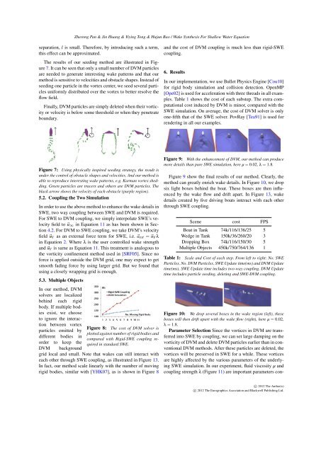
and the cost of DVM coupling is much less than rigid-SWE
coupling.
6. Results
In our implementation, we use Bullet Physics Engine [Cou10]
for rigid body simulation and collision detection. OpenMP
[Ope02] is used for acceleration with three threads in all examples.
Table 1 shows the cost of each substep. The extra computational
cost induced by DVM is minor, compared with the
SWE simulation. On average, the cost of DVM solver is only
one-fifth that of the SWE solver. PovRay [Tea91] is used for
rendering in all our examples.
Figure 7: Using physically inspired seeding strategy, the result is
under the control of obstacle shapes and velocities. And our method is
able to reproduce interesting wake patterns, e.g. Karman vortex shedding.
Green particles are tracers and others are DVM particles. The
black arrow shows the velocity of each obstacle (purple region).
5.2. Coupling the Two Simulation
In order to use the above method to enhance the wake details in
SWE, two way coupling between SWE and DVM is required.
For SWE to DVM coupling, we simply interpolate SWE’s velocity
field to ⃗u ∞ in Equation 11 as has been shown in Section
4.2. For DVM to SWE coupling, we take DVM’s velocity
field ⃗u V as an external force term for SWE, i.e. ⃗a ext = ⃗u V λ
in Equation 2. Where λ is the user controlled wake strength
and ⃗u V is same as Equation 11. This treatment is analogous to
the vorticity confinement method used in [SRF05]. Since no
force is applied outside the DVM grid, one may expect to get
smooth fading force by using larger grid. But we found that
using a closely wrapping grid is enough.
5.3. Multiple Objects
In our method, DVM
solvers are localized
behind each rigid
body. If multiple bodies
exist, we choose
to ignore the interaction
between vortex
particles emitted by
different bodies in
order to keep the
Figure 8: The cost of DVM solver is
plotted against number of rigid bodies and
compared with Rigid-SWE coupling required
in standard SWE.
DVM background
grid local and small. Note that wakes can still interact with
each other through SWE coupling, as illustrated in Figure 13.
In fact, our method scale linearly with the number of moving
rigid bodies, similar with [YHK07], as is shown in Figure 8
Figure 9: With the enhancement of DVM, our method can produce
more details than pure SWE simulation, here µ = 0.02, λ = 1.8.
Figure 9 show the final results of our method. Clearly, the
method can greatly enrich wake details. In Figure 10, we drop
six light boxes behind the boat. These boxes are then influenced
by the wake flow and drift apart. In Figure 13, wake
details created by five driving boats interact with each other
through SWE coupling.
Scene cost FPS
Boat in Tank 74k/116/136/25 5
Wedge in Tank 150k/36/260/20 3
Dropping Box 74k/116/150/30 5
Multiple Objects 450k/750/764/136 1
Table 1: Scale and Cost of each step. From left to right: No. SWE
Particles, No. DVM Particles, SWE Update time(ms) and DVM Update
time(ms). SWE Update time includes two-way coupling. DVM Update
time includes particle seeding, deleting and SWE-DVM coupling.
Figure 10: We drop several boxes in the wake region (left), these
boxes will then drift apart with the wake flow (right), here µ = 0.02,
λ = 1.8.
Parameter Selection Since the vortices in DVM are transferred
into SWE by coupling, we can set large damping on the
vorticity of DVM and delete DVM particles earlier than in conventional
DVM methods. After these particles are deleted, the
vortices will be preserved in SWE for a while. These vortices
are highly affected by the various parameters of the underlying
SWE simulation. In our experiment, fluid viscosity µ and
coupling strength λ (Figure 11) are important parameters conc○
2012 The Author(s)
c○ 2012 The Eurographics Association and Blackwell Publishing Ltd.