Wake Synthesis For Shallow Water Equation - Department of ...
Wake Synthesis For Shallow Water Equation - Department of ...
Wake Synthesis For Shallow Water Equation - Department of ...

Create successful ePaper yourself
Turn your PDF publications into a flip-book with our unique Google optimized e-Paper software.
Pacific Graphics 2012<br />
C. Bregler, P. Sander, and M. Wimmer<br />
(Guest Editors)<br />
Volume 31 (2012), Number 7<br />
The definitive version is available at http://diglib.eg.org/ and http://onlinelibrary.wiley.com/.<br />
<strong>Wake</strong> <strong>Synthesis</strong> <strong>For</strong> <strong>Shallow</strong> <strong>Water</strong> <strong>Equation</strong><br />
Zherong Pan 1 Jin Huang †1 Yiying Tong 2 Hujun Bao 1<br />
1 State Key Lab <strong>of</strong> CAD&CG, Zhejiang University, China, 2 Michigan State University, USA<br />
Abstract<br />
In fluid animation, wake is one <strong>of</strong> the most important phenomena usually seen when an object is moving relative to<br />
the flow. However, in current shallow water simulation for interactive applications, this effect is greatly smeared<br />
out. In this paper, we present a method to efficiently synthesize these wakes. We adopt a generalized SPH method<br />
for shallow water simulation and two way solid fluid coupling. In addition, a 2D discrete vortex method is used<br />
to capture the detailed wake motions behind an obstacle, enriching the motion <strong>of</strong> SWE simulation. Our method is<br />
highly efficient since only 2D simulation is required. Moreover, by using a physically inspired procedural approach<br />
for particle seeding, DVM particles are only created in the wake region. Therefore, very few particles are required<br />
while still generating realistic wake patterns. When coupled with SWE, we show that these patterns can be seen<br />
using our method with marginal overhead.<br />
Categories and Subject Descriptors (according to ACM CCS): I.3.7 [Computer Graphics]: Three Dimensional Graphics<br />
and Realism—Animation<br />
1. Introduction<br />
Liquid animation is among the most stunning visual effects<br />
in computer graphics. The field has witnessed great progress<br />
in the last ten years, readily handling viscous flow, surface<br />
tension and multiphase scenarios. However, a full 3D Navier-<br />
Stokes simulation is <strong>of</strong>ten costly for interactive applications<br />
like real time games. Instead, the shallow water equation<br />
(SWE) serves as a cheap alternative for flow with large horizontal<br />
to vertical scale ratio. By using depth averaged velocity<br />
field, one dimension is effectively removed and the costly<br />
pressure projection is not required.<br />
However, it is not fluid itself but the relative motion <strong>of</strong> fluid<br />
and solid body that accounts for the most interesting effects in<br />
this field such as wake flow and von Karman vortex shedding,<br />
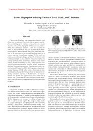
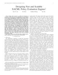
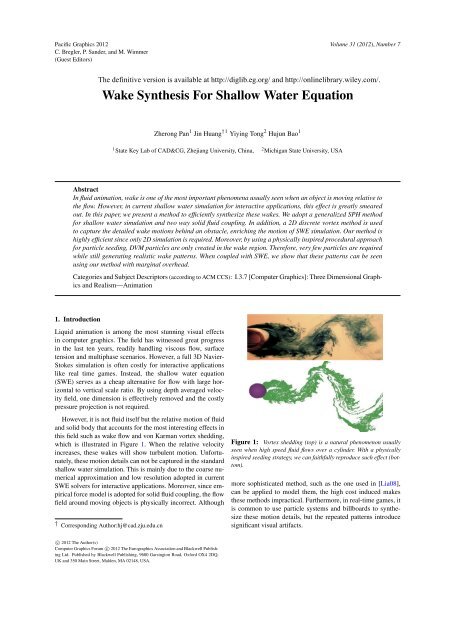
which is illustrated in Figure 1. When the relative velocity Figure 1: Vortex shedding (top) is a natural phenomenon usually<br />
increases, these wakes will show turbulent motion. Unfortunately,<br />
these motion details can not be captured in the standard<br />
seen when high speed fluid flows over a cylinder. With a physically<br />
inspired seeding strategy, we can faithfully reproduce such effect (bottom).<br />
shallow water simulation. This is mainly due to the coarse numerical<br />
approximation and low resolution adopted in current<br />
SWE solvers for interactive applications. Moreover, since empirical<br />
force model is adopted for solid fluid coupling, the flow can be applied to model them, the high cost induced makes<br />
more sophisticated method, such as the one used in [Lia08],<br />
field around moving objects is physically incorrect. Although these methods impractical. Furthermore, in real-time games, it<br />
is common to use particle systems and billboards to synthesize<br />
these motion details, but the repeated patterns introduce<br />
† Corresponding Author:hj@cad.zju.edu.cn significant visual artifacts.<br />
c○ 2012 The Author(s)<br />
Computer Graphics <strong>For</strong>um c○ 2012 The Eurographics Association and Blackwell Publishing<br />
Ltd. Published by Blackwell Publishing, 9600 Garsington Road, Oxford OX4 2DQ,<br />
UK and 350 Main Street, Malden, MA 02148, USA.
Zherong Pan & Jin Huang & Yiying Tong & Hujun Bao / <strong>Wake</strong> <strong>Synthesis</strong> <strong>For</strong> <strong>Shallow</strong> <strong>Water</strong> <strong>Equation</strong><br />
In this paper, we propose a method to synthesize the wakes<br />
behind moving objects. In our approach, we use two different<br />
representations for the fluid, one for conventional SWE and<br />
the other for wake detail enhancement. <strong>For</strong> SWE simulation,<br />
we adopt a generalized SPH method recently introduced in<br />
[SBC ∗ 11] and [LH10]. <strong>For</strong> wake detail enhancement, we use<br />
a localized 2D version <strong>of</strong> the discrete vortex method (DVM)<br />
similar to [PK05] around each moving object. However, DVM<br />
requires a careful placement <strong>of</strong> the particles to resolve the flow<br />
field. Therefore, we propose a physically inspired procedural<br />
method for particle seeding. We show that this effectively concentrates<br />
the particles on the wake region and greatly reduces<br />
the number <strong>of</strong> particles required in DVM, while still generating<br />
phenomena like vortex shedding and turbulence as relative<br />
velocity increases. In the field <strong>of</strong> computational fluid dynamics,<br />
a similar idea is adopted in [HA97]. In order to couple<br />
the two simulations, we use SWE’s velocity field as the ambient<br />
flow for DVM. While, DVM’s velocity field is taken as an<br />
external force term on SWE. This is similar to the famous vorticity<br />
confinement method [FSJ01] widely used in grid based<br />
solvers.<br />
The two simulations used in our method are both 2D, so the<br />
method is efficient enough for real-time applications. Our vortex<br />
particle seeding method is physically inspired and sensitive<br />
to both the velocities and shapes <strong>of</strong> obstacles. We show that<br />
this method is capable <strong>of</strong> generating different wake patterns<br />
including Karman vortex shedding. Moreover, the method is<br />
independent <strong>of</strong> the underlying SWE implementation and is applicable<br />
to a conventional grid based SWE solver as well. Although<br />
we take some non-physically based assumptions, we<br />
show that our method achieves good balance between visual<br />
effect and performance which is the main goal <strong>of</strong> this work. In<br />
short, the contributions are:<br />
• Efficient enrichment <strong>of</strong> the wake details for SWE simulation.<br />
• Physically inspired seeding strategy for wake synthesis.<br />
• Flexible integration into various SWE implementations.<br />
2. Related Works<br />
Three Dimensional Fluid Simulation Full 3D grid based<br />
Navier-Stokes simulation has gained popularity since the work<br />
<strong>of</strong> [Sta99] and [FF01]. And a number <strong>of</strong> extensions have been<br />
proposed in works such as [HK05], [LGF04] and [LSSF06].<br />
However, these methods are still too slow for interactive applications.<br />
Instead, particle-based methods, like the famous<br />
Smoothed Particle Hydrodynamics introduced in [MCG03],<br />
can achieve real-time performance with lower memory cost.<br />
Later, 3D simulations were coupled with 2D ones to get better<br />
performance in the work <strong>of</strong> [IGLF06]. And real-time performance<br />
has been achieved by [CM11] using such technique, but<br />
the whole GPU is occupied in their method. Therefore, these<br />
methods are still impractical for interactive applications.<br />
Two Dimensional Fluid Simulation Game developers usually<br />
find good balance between surface details and simulation<br />
cost by using 2D heightfield based fluid simulation. The<br />
most popular method <strong>of</strong> this kind is the shallow water equation<br />
(SWE) and wave equation (WE). SWE provides more<br />
information than WE by taking advection into consideration.<br />
This method was introduced to computer graphics for the<br />
first time by [KM90]. Numerous extensions have been proposed<br />
later on. [OH95] used a particle system to enhance the<br />
splashing effect. [FM96] and [CLHM97] introduced solid fluid<br />
coupling. [TMFSG07] synthesized breaking wave effect for<br />
SWE. [TSS ∗ 07] simulated bubbly flow under SWE framework.<br />
[LO07] proposed a new advection scheme to reduce numerical<br />
viscosity. Recently, [CM10] proposed an even better<br />
SWE scheme and coupled several techniques to achieve better<br />
visual quality. But they only used billboards and particle systems<br />
for wake details. Apart from grid-based solvers, [LH10]<br />
and [SBC ∗ 11] showed that a standard 2D SPH method can be<br />
used for SWE simulation through a generalized pressure definition.<br />
In this paper, we adopt their method as our main SWE<br />
solver.<br />
Instead <strong>of</strong> shallow water equation, [YHK07] showed that<br />
water equation can also provide plausible results. However,<br />
since this method don’t describe the entire flow field, interesting<br />
phenomenon such as whirlpool can not be represented.<br />
Therefore, we choose to adopt SWE as our underlying solver.<br />
Although SWE is physically based modelling, the solid fluid<br />
coupling methods currently used are mostly based on empirical<br />
models. [CLHM97] used movable boundary condition to<br />
achieve one way solid to fluid coupling. Later, [YHK07] proposed<br />
an empirical model for two way coupling, which is also<br />
used in SPH based method <strong>of</strong> [SBC ∗ 11]. All these methods are<br />
physically inaccurate in modelling relative motion <strong>of</strong> obstacle<br />
and fluid, result in smeared out wake details.<br />
Discrete Vortex Method (DVM) This kind <strong>of</strong> method is<br />
based on the curl form <strong>of</strong> Navier-Stokes equation. However,<br />
since the pioneering work <strong>of</strong> [GLG ∗ 95], DVM has not gained<br />
much popularity due to its various limitations, e.g. vorticity<br />
stretching and tiling causes numerical instability in 3D; particle<br />
placement is tricky to resolve the flow field; boundary<br />
condition is hard to enforce. A more sophisticated version <strong>of</strong><br />
DVM is introduced by [PK05], a 2D version similar to which<br />
is used in this paper.<br />
Turbulence <strong>Synthesis</strong> Turbulence modelling has a long history<br />
in fluid dynamics, for which [Pop00] provides an introduction.<br />
In computer graphics, a variety <strong>of</strong> methods have been<br />
proposed to synthesize the small scale details. [FSJ01] proposed<br />
vorticity confinement, but this approach still depends<br />
on the underlying grid resolution. Later, [SRF05] alleviated<br />
these problems through a hybrid vortex particle and grid based<br />
method but particle seeding in their method is random. Recent<br />
works such as [NSCL08], [SB08] and [PTSG09] models<br />
turbulence generation and energy transfer in a more accurate<br />
way. Since these methods adopt a stochastic approach, they<br />
cannot model periodic patterned motions that we focus on.<br />
c○ 2012 The Author(s)<br />
c○ 2012 The Eurographics Association and Blackwell Publishing Ltd.
Zherong Pan & Jin Huang & Yiying Tong & Hujun Bao / <strong>Wake</strong> <strong>Synthesis</strong> <strong>For</strong> <strong>Shallow</strong> <strong>Water</strong> <strong>Equation</strong><br />
Other works, e.g. [ZYF10] and [YYF12], incorporate similar<br />
idea into particle based fluid solvers. All these methods base<br />
themselves on a physically correct background mean flow. Unfortunately,<br />
in our case, the background SWE flow field is far<br />
from accurate around moving objects, making these methods<br />
inapplicable.<br />
3. Overview<br />
Our method is a hybrid version (Algorithm 1) <strong>of</strong> shallow water<br />
equation (SWE) and discrete vortex method (DVM). In the following<br />
sections, we elaborate each substep in one simulation<br />
iteration. In Section 4, we introduce the basic SWE and DVM<br />
solvers. In Section 5, we describe our method for physically<br />
inspired particle seeding, deleting and SWE-DVM coupling.<br />
Final results and analysis are given in section 6 and 7.<br />
Algorithm 1 Simulation Loop<br />
Step SWE and couple with rigid body.<br />
for each rigid body do<br />
Interpolate SWE’s velocity field to DVM.<br />
Step DVM and perform particle seeding, deleting.<br />
Apply DVM’s velocity field as external force on SWE.<br />
end for<br />
4. SWE and DVM Simulation<br />
In this section, we give a brief description <strong>of</strong> the two simulation<br />
methods. <strong>For</strong> the SWE simulation, we adopt the generalized<br />
SPH scheme <strong>of</strong> [SBC ∗ 11]. <strong>For</strong> the DVM simulation, a<br />
simplified version <strong>of</strong> [PK05] is used.<br />
4.1. <strong>Shallow</strong> <strong>Water</strong> Simulation<br />
The shallow water equation (SWE) is the depth averaged version<br />
<strong>of</strong> the Navier-Stokes equation. It can be written as:<br />
Dh<br />
Dt<br />
= −h∇ ·⃗u (1)<br />
D⃗u<br />
Dt<br />
= −g∇(h + H) +⃗a ext, (2)<br />
where h is the water column height, H is the height <strong>of</strong> bottom<br />
terrain, g is the gravitational acceleration, ⃗u is the horizontal<br />
velocity and ⃗a ext represents the external force term.<br />
Currently, most SWE solvers are grid based. These solvers<br />
usually suffer from detail loss due to numerical viscosity and<br />
high memory cost. Therefore, we choose to adopt a generalized<br />
SPH method recently proposed by [SBC ∗ 11] and [LH10].<br />
The method preserves volume naturally and has lower memory<br />
cost. Here we briefly review this approach.<br />
The basic discretization used in SPH is the smoothed kernel<br />
interpolation. Given an arbitrary set <strong>of</strong> particles each carrying<br />
physics property A, we can evaluate this property at any location⃗x<br />
through the following equation:<br />
A(⃗x) = ∑<br />
j<br />
m j<br />
ρ j<br />
A j W(⃗x −⃗x j ,l), (3)<br />
where m is the constant particle mass, ρ is the fluid density<br />
and W(⃗x) is the interpolation kernel function. <strong>For</strong> the choice<br />
<strong>of</strong> these kernel functions, we follow [MCG03]. One advantage<br />
<strong>of</strong> this formulation is that differential operators need only to<br />
be applied on the kernels as follows:<br />
∇A(⃗x) = ∑<br />
j<br />
m j<br />
ρ j<br />
A j ∇W(⃗x −⃗x j ,l) (4)<br />
∇ 2 m j<br />
A(⃗x) = ∑ A j ∇ 2 W(⃗x −⃗x j ,l). (5)<br />
j ρ j<br />
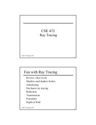
To extend an existing 2D SPH solver for SWE, the key idea<br />
is to take the particle density in standard SPH as water column<br />
height. As in Figure 2, denser particles correspond to higher<br />
water column. Therefore, water column mass m i and height<br />
h i0 are defined on each particle and kept constant across the<br />
simulation. In this way, mass is trivially preserved and the continuity<br />
<strong>Equation</strong> 1 can be discarded. <strong>Equation</strong> 2 is easy to discretize<br />
using <strong>Equation</strong> 3 and 4:<br />
h a i<br />
∂⃗u i<br />
∂t<br />
= ∑<br />
j<br />
= −g∑<br />
j<br />
m j<br />
ρ 0<br />
W(⃗x i −⃗x j ,l) (6)<br />
m j<br />
h a ρ 0 h<br />
j∇W(⃗x i −⃗x j ,l) − g∇H +⃗a ext, (7)<br />
j0<br />
where h a is the averaged water column height updated in each<br />
timestep. However, merely using the above equation will lead<br />
to numerical instability. Therefore, we add a viscosity term following<br />
[MCG03]:<br />
∂⃗u i<br />
∂t<br />
= µ∑<br />
j<br />
m j<br />
(⃗u j −⃗u i )∇ 2 W(⃗x i −⃗x j ,l). (8)<br />
ρ 0 h j0<br />
Note that we use the summation formulation (<strong>Equation</strong> 6) for<br />
h a , which is more stable than the differential update formulation<br />
used in the original work <strong>of</strong> [SBC ∗ 11] and [LH10]. This<br />
formulation is also used in [AS05] to solve SWE.<br />
Based on the above solver, two<br />
way solid fluid coupling can be<br />
approximated using an empirical<br />
force model. <strong>For</strong> fluid to solid coupling,<br />
[SBC ∗ 11] used three force<br />
terms on each rigid body, i.e. buoyant,<br />
lift and drag force. Buoyant<br />
force is calculated by tracing two<br />
rays from each particle to find the<br />
amount <strong>of</strong> water displaced. Lift<br />
and drag forces are applied following<br />
[YHK07]. <strong>For</strong> solid to fluid<br />
Figure 2: 1D illustration<br />
<strong>of</strong> SPH based SWE discretization.<br />
Denser particles<br />
correspond to higher<br />
water column.<br />
coupling, [SBC ∗ 11] used a force model based on fully elastic<br />
collision.<br />
4.2. Discrete Vortex Method<br />
DVM is known for its ability to create rich flow details using<br />
very few particles. The governing equation <strong>of</strong> DVM is the curl<br />
form <strong>of</strong> Navier-Stokes equation written as:<br />
∂⃗ω<br />
∂t<br />
= −(⃗u · ∇)⃗ω + (∇⃗u) ·⃗ω + µ∇ 2 ⃗ω. (9)<br />
c○ 2012 The Author(s)<br />
c○ 2012 The Eurographics Association and Blackwell Publishing Ltd.
Zherong Pan & Jin Huang & Yiying Tong & Hujun Bao / <strong>Wake</strong> <strong>Synthesis</strong> <strong>For</strong> <strong>Shallow</strong> <strong>Water</strong> <strong>Equation</strong><br />
Since we use the 2D version <strong>of</strong> DVM, the vorticity ⃗ω reduces<br />
to a scalar since only the ⃗Z component is nonzero and the<br />
stretching term <strong>of</strong> (∇⃗u) ·⃗ω, which frequently causes numerical<br />
instability in 3D cases, vanishes. In this way, <strong>Equation</strong> 9<br />
can be simplified to give:<br />
∂ω<br />
∂t<br />
= −(⃗u · ∇)ω + µ∇ 2 ω. (10)<br />
To discretize this equation, DVM uses a set <strong>of</strong> lagrangian<br />
particles each carrying a vorticity ω i . Under this representation,<br />
a split-step method can be employed by considering the<br />
two terms right handle side <strong>of</strong> <strong>Equation</strong> 10 (advection, diffusion)<br />
in separate substeps to update the position and vorticity<br />
<strong>of</strong> each particle.<br />
<strong>For</strong> the advection substep, we have to calculate the velocity<br />
field ⃗u. In DVM, velocity field consists <strong>of</strong> three terms [PK05],<br />
giving:<br />
⃗u = ⃗u ∞ +⃗u V +⃗u P . (11)<br />
Here, ⃗u ∞ stands for the velocity <strong>of</strong> ambient flow. In our<br />
method, we interpolate SWE’s velocity field to DVM for this<br />
term. ⃗u V stands for velocity induced by the vorticity carried<br />
on DVM particles. Finally, ⃗u P stands for the velocity induced<br />
by boundary condition. Since we use large vorticity damping<br />
in DVM, particles are deleted quickly and seldom penetrate<br />
boundary. So, we neglect term ⃗u P .<br />
The most tricky part <strong>of</strong> DVM lies in the approximation <strong>of</strong>⃗u V<br />
term. Here, a velocity field is reconstructed from the vorticity<br />
field through Biot-Savart integration, whose discretized form<br />
can be written as:<br />
N<br />
⃗u V (x) = − ∑ V ((⃗x −⃗x i) ×⃗ω i )q(‖⃗x −⃗x i ‖/σ)<br />
i=0 ‖⃗x −⃗x i ‖ 2 , (12)<br />
where V is the particle volume kept constant across simulation,<br />
σ is the smoothing range, q(λ) = 2π 1 (1 − exp(−λ2 /2))<br />
and ⃗ω i = ω⃗Z. Performing this summation directly on every<br />
particle location will cost O(N 2 ). Instead, [PK05] used the Fast<br />
Multipole Method [GR87, AG91] to accelerate this process to<br />
O(NlogN) or even O(N).<br />
However, the constant factor in such method is large. Since<br />
the number <strong>of</strong> particles used in our case is small and high accuracy<br />
is not required, a simple TreeCode [LK01] will suffice.<br />
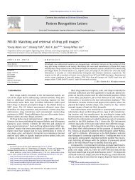
<strong>For</strong> each moving object,<br />
we create a localized background<br />
grid behind the object<br />
and evaluate velocity<br />
at every grid point. As illustrated<br />
in Figure 3, the Figure 3: A wedge moving in<br />
grid closely wrapping the flow. DVM particles are seeded behind<br />
it (red). And a localized grid is<br />
DVM particles is updated<br />
created wrapping these particles.<br />
in each timestep. Therefore,<br />
the DVM grid size is independent <strong>of</strong> the entire area <strong>of</strong> the<br />
scene. To update the positions <strong>of</strong> DVM particles, we interpolate<br />
velocities from the grid for these particles as well.<br />
<strong>For</strong> the diffusion substep, [PK05] adopted the method <strong>of</strong><br />
particle strength exchange (PSE), where each vortex particle<br />
exchanges some <strong>of</strong> the vorticity with surrounding particles in<br />
each timestep. However, evaluating this term requires a neighbour<br />
search. Instead, we choose to simply set a large global<br />
damping on the vorticity.<br />
5. <strong>Wake</strong> <strong>Synthesis</strong><br />
When a rigid body is moving in the fluid, a boundary layer will<br />
form around the body where the behaviour <strong>of</strong> fluid is under<br />
the combined influence <strong>of</strong> the ambient mean flow and surface<br />
friction. In this region, vorticity is created and confined. These<br />
vortices will then detach from the surface and be emitted into<br />
the mean flow, generating interesting wake motion behind the<br />
body. Depending on the magnitude <strong>of</strong> relative velocity, this<br />
motion can be laminar or turbulent.<br />
Although DVM is efficient in describing and preserving<br />
vorticity, the placement <strong>of</strong> DVM particles is a challenging<br />
problem. To properly reproduce periodic wake patterns like<br />
Karman vortex shedding, the naive random seeding strategy<br />
used by [SRF05] will not work. In this section, we describe<br />
our method <strong>of</strong> particle seeding and SWE-DVM coupling. The<br />
method can effectively reproduce various wake patterns with<br />
few DVM particles.<br />
5.1. Physically Inspired Particle Seeding and Deleting<br />
Since very few particles are used, each one has to be carefully<br />
placed to resolve the flow field in DVM. [PK05] seeded<br />
two rows <strong>of</strong> particles with different sign <strong>of</strong> vorticity to create<br />
a steady and constant mean flow. However, since obstacles in<br />
SWE may move in arbitrary direction, their method is not applicable<br />
in our case.<br />
We, instead, propose a physically inspired procedural<br />
method for particle seeding, which is sensitive to object shapes<br />
and velocities. The method is based on the boundary layer theory<br />
<strong>of</strong> CFD. In real life, surface friction causes the flow velocity<br />
to be zero at wall, creating a boundary layer. On the back<br />
face <strong>of</strong> the obstacle, velocity decreases and pressure increases<br />
along mean flow direction, which is called adverse pressure<br />
gradient. When the mean flow travels long enough under such<br />
pressure pr<strong>of</strong>ile, vortices are created and confined. They will<br />
finally detach from body surface and be emitted into the ambient<br />
flow field. <strong>For</strong> more details on boundary layer theory,<br />
see [SG00].<br />
We take the simple assumption that every rigid body is convex,<br />
common in real-time physics engines. To model boundary<br />
layer separation, detecting points are placed on all the edges <strong>of</strong><br />
a rigid body. In addition, with each detecting point, two potentials<br />
are defined corresponding to each incident face. We accumulate<br />
these potentials in each timestep. When a threshold<br />
is reach by either <strong>of</strong> the potentials, a vortex is seeded in the<br />
downstream and the potential is reset for next seeding.<br />
c○ 2012 The Author(s)<br />
c○ 2012 The Eurographics Association and Blackwell Publishing Ltd.
Zherong Pan & Jin Huang & Yiying Tong & Hujun Bao / <strong>Wake</strong> <strong>Synthesis</strong> <strong>For</strong> <strong>Shallow</strong> <strong>Water</strong> <strong>Equation</strong><br />
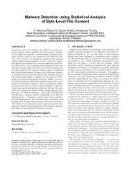
will contribute to potentials. <strong>For</strong> example, if ⃗u pr j<br />
rel lies in region<br />
3, we decide that vorticity created and confined on the red face<br />
will meet adverse pressure pr<strong>of</strong>ile on the green face. Therefore,<br />
E 1 increases for the red face and E 2 decreases for the<br />
green face. When either <strong>of</strong> the above two potentials reaches T ,<br />
a predefined global threshold, we assume that a vortex should<br />
detach from the corresponding face and seed one vortex.<br />
Figure 4: Left (front view): Separation detecting point (white), seeding<br />
potentials (yellow), two intersecting lines (blue) and XY-projected<br />
vectors. Right (top view): If relative velocity lies in region 3, E 1 increases<br />
and E 2 decreases.<br />
Separation Detection <strong>For</strong> every edge <strong>of</strong> a convex rigid<br />
body, we place a detecting point P d at the center. And two<br />
seeding potentials, E 1 and E 2 , are defined one for each <strong>of</strong> the<br />
incident face. Since we work on a 2D version <strong>of</strong> DVM, normal<br />
vectors are projected onto the XY-Plane and the projected<br />
mean tangent is calculated at each timestep. We use superscript<br />
pr j for the XY-Projected vectors. This is illustrated in Figure 4<br />
(left).<br />
Very small vortices are visually neglectable and the average<br />
vortex radius is related to the characteristic length <strong>of</strong> the body.<br />
So, we choose to only capture vortices with radius R = AL,<br />
where A is a user defined value and L is the average <strong>of</strong> three<br />
edge length <strong>of</strong> the bounding box in each axis. In our experiment,<br />
R affects the behaviour <strong>of</strong> wake details slightly as long<br />
as 0.1 ≤ A ≤ 0.3. We use A = 0.15 in all our examples. Moreover,<br />
adverse pressure pr<strong>of</strong>ile can only occur on the back face<br />
<strong>of</strong> the body. And the seeding possibility is proportional to the<br />
tangent velocity magnitude according to [PTSG09]. To model<br />
this effect, we choose to accumulate E 1 and E 2 above through<br />
the following equations:<br />
E 1 (t + ∆t) = max(exp(( u1 E f f<br />
M − 1)∆t)E 1(t),1) (13)<br />
E 2 (t + ∆t) = max(exp(( u2 E f f<br />
M − 1)∆t)E 2(t),1), (14)<br />
where M > 0 is the minimal velocity magnitude for vortex<br />
seeding. Although these two equations are not physically<br />
based, they give natural results and provide enough controllability<br />
over the particle seeding frequency. Here u 1 E f f and u2 E f f<br />
are defined as:<br />
{<br />
u 1 pr j abs(⃗u<br />
E f f =<br />
rel ·⃗t pr j )<br />
0 otherwise<br />
{<br />
u 2 pr j abs(⃗u<br />
E f f =<br />
rel ·⃗t pr j )<br />
0 otherwise,<br />
where ⃗u pr j<br />
rel<br />
if ⃗u pr j<br />
rel lies in region 3<br />
if ⃗u pr j<br />
rel lies in region 1<br />
(15)<br />
(16)<br />
= ⃗u pr j<br />
F −⃗upr j<br />
B is the projected relative velocity at<br />
that point and⃗t pr j is the projected mean tangent as in Figure 4.<br />
In this way, only the relative velocity which meets adverse<br />
pressure pr<strong>of</strong>ile, i.e. lies in region 1 and 3 in Figure 4 (right),<br />
Depending on the topology <strong>of</strong> obstacle mesh, several edges<br />
may have projected positions close to each other, emitting<br />
overlapped vortices. Therefore, although we accumulate potentials<br />
on all edges, we only emit vortices on edges intersecting<br />
the SWE surface. Afterwards, all the potentials on detecting<br />
point P d whose position ⃗x satisfies ‖⃗x pr j −⃗x pr j<br />
0 ‖ < R are<br />
reset to one for next seeding, where ⃗x pr j<br />
0 is the projected detecting<br />
point from which a vortex has just been seeded. This is<br />
analogous to [PTSG09].<br />
Particle Seeding and Deleting<br />
When the above step determines<br />
that a vortex should be emitted<br />
from a detecting point P d , we have<br />
to find the seeding position P s and<br />
strength <strong>of</strong> the vortex ω. To do this,<br />
we observe that the seeded vortex<br />
should be righT outside the body<br />
with no collision. Moreover, the<br />
vortex should have one boundary Figure 5: When the<br />
point attached to the mean flow. potential (yellow) <strong>of</strong> one<br />
Therefore, we perform a continuous<br />
collision detection (CCD) be-<br />
detecting point (gray)<br />
excesses threshold T , we<br />
find the seeding position by<br />
tween the body and a sphere with<br />
CCD along the gray dashed<br />
radius R along the direction <strong>of</strong>⃗u pr j<br />
rel line, which is parallel to the<br />
to find the closest point satisfying<br />
relative velocity around the<br />
the above requirements as il-<br />
boat (thick blue arrows).<br />
lustrated in Figure 5. Since we take the convex body assumption,<br />
this vortex will not be blocked by other part <strong>of</strong> the body<br />
and the CCD can be performed very efficiently using such algorithms<br />
as GJK [GJK88].<br />
In order to determine the strength ω <strong>of</strong> the vortex, a simple<br />
approximation is ω = ‖⃗u pr j<br />
rel ‖/R. However, we propose to add<br />
a fading term to this equation, giving:<br />
ω = ‖⃗u pr j<br />
rel ‖exp(−l/A)/R, (17)<br />
where l is an additional piece <strong>of</strong> information acquired during<br />
the CCD, which is the distance between detecting and seeding<br />
position projected on ⃗u pr j<br />
rel . This can be written as:<br />
As in Figure 6, when<br />
a streamlined object,<br />
which usually suppress<br />
vortex separation, is<br />
moving in the flow, l<br />
is large. While for a<br />
sharp corner, which<br />
usually amplify vortex<br />
⃗u pr j<br />
rel<br />
l = abs((⃗P d −⃗P s) ·<br />
‖⃗u pr j ). (18)<br />
rel ‖<br />
Figure 6: A streamlined object results<br />
in large l (left), while a sharp corner<br />
results in small l (right).<br />
c○ 2012 The Author(s)<br />
c○ 2012 The Eurographics Association and Blackwell Publishing Ltd.
Zherong Pan & Jin Huang & Yiying Tong & Hujun Bao / <strong>Wake</strong> <strong>Synthesis</strong> <strong>For</strong> <strong>Shallow</strong> <strong>Water</strong> <strong>Equation</strong><br />
separation, l is small. Therefore, by introducing such a term,<br />
this effect can be approximated.<br />
The results <strong>of</strong> our seeding method are illustrated in Figure<br />
7. It can be seen that only a small number <strong>of</strong> DVM particles<br />
are needed to generate interesting wake patterns and that our<br />
method is sensitive to velocities and obstacle shapes. Instead <strong>of</strong><br />
seeding one particle in the vortex center, we seed several particles<br />
uniformly distributed over the vortex to better resolve the<br />
flow field.<br />
Finally, DVM particles are simply deleted when their vorticity<br />
or velocity is below some threshold or when they penetrate<br />
boundary.<br />
and the cost <strong>of</strong> DVM coupling is much less than rigid-SWE<br />
coupling.<br />
6. Results<br />
In our implementation, we use Bullet Physics Engine [Cou10]<br />
for rigid body simulation and collision detection. OpenMP<br />
[Ope02] is used for acceleration with three threads in all examples.<br />
Table 1 shows the cost <strong>of</strong> each substep. The extra computational<br />
cost induced by DVM is minor, compared with the<br />
SWE simulation. On average, the cost <strong>of</strong> DVM solver is only<br />
one-fifth that <strong>of</strong> the SWE solver. PovRay [Tea91] is used for<br />
rendering in all our examples.<br />
Figure 7: Using physically inspired seeding strategy, the result is<br />
under the control <strong>of</strong> obstacle shapes and velocities. And our method is<br />
able to reproduce interesting wake patterns, e.g. Karman vortex shedding.<br />
Green particles are tracers and others are DVM particles. The<br />
black arrow shows the velocity <strong>of</strong> each obstacle (purple region).<br />
5.2. Coupling the Two Simulation<br />
In order to use the above method to enhance the wake details in<br />
SWE, two way coupling between SWE and DVM is required.<br />
<strong>For</strong> SWE to DVM coupling, we simply interpolate SWE’s velocity<br />
field to ⃗u ∞ in <strong>Equation</strong> 11 as has been shown in Section<br />
4.2. <strong>For</strong> DVM to SWE coupling, we take DVM’s velocity<br />
field ⃗u V as an external force term for SWE, i.e. ⃗a ext = ⃗u V λ<br />
in <strong>Equation</strong> 2. Where λ is the user controlled wake strength<br />
and ⃗u V is same as <strong>Equation</strong> 11. This treatment is analogous to<br />
the vorticity confinement method used in [SRF05]. Since no<br />
force is applied outside the DVM grid, one may expect to get<br />
smooth fading force by using larger grid. But we found that<br />
using a closely wrapping grid is enough.<br />
5.3. Multiple Objects<br />
In our method, DVM<br />
solvers are localized<br />
behind each rigid<br />
body. If multiple bodies<br />
exist, we choose<br />
to ignore the interaction<br />
between vortex<br />
particles emitted by<br />
different bodies in<br />
order to keep the<br />
Figure 8: The cost <strong>of</strong> DVM solver is<br />
plotted against number <strong>of</strong> rigid bodies and<br />
compared with Rigid-SWE coupling required<br />
in standard SWE.<br />
DVM background<br />
grid local and small. Note that wakes can still interact with<br />
each other through SWE coupling, as illustrated in Figure 13.<br />
In fact, our method scale linearly with the number <strong>of</strong> moving<br />
rigid bodies, similar with [YHK07], as is shown in Figure 8<br />
Figure 9: With the enhancement <strong>of</strong> DVM, our method can produce<br />
more details than pure SWE simulation, here µ = 0.02, λ = 1.8.<br />
Figure 9 show the final results <strong>of</strong> our method. Clearly, the<br />
method can greatly enrich wake details. In Figure 10, we drop<br />
six light boxes behind the boat. These boxes are then influenced<br />
by the wake flow and drift apart. In Figure 13, wake<br />
details created by five driving boats interact with each other<br />
through SWE coupling.<br />
Scene cost FPS<br />
Boat in Tank 74k/116/136/25 5<br />
Wedge in Tank 150k/36/260/20 3<br />
Dropping Box 74k/116/150/30 5<br />
Multiple Objects 450k/750/764/136 1<br />
Table 1: Scale and Cost <strong>of</strong> each step. From left to right: No. SWE<br />
Particles, No. DVM Particles, SWE Update time(ms) and DVM Update<br />
time(ms). SWE Update time includes two-way coupling. DVM Update<br />
time includes particle seeding, deleting and SWE-DVM coupling.<br />
Figure 10: We drop several boxes in the wake region (left), these<br />
boxes will then drift apart with the wake flow (right), here µ = 0.02,<br />
λ = 1.8.<br />
Parameter Selection Since the vortices in DVM are transferred<br />
into SWE by coupling, we can set large damping on the<br />
vorticity <strong>of</strong> DVM and delete DVM particles earlier than in conventional<br />
DVM methods. After these particles are deleted, the<br />
vortices will be preserved in SWE for a while. These vortices<br />
are highly affected by the various parameters <strong>of</strong> the underlying<br />
SWE simulation. In our experiment, fluid viscosity µ and<br />
coupling strength λ (Figure 11) are important parameters conc○<br />
2012 The Author(s)<br />
c○ 2012 The Eurographics Association and Blackwell Publishing Ltd.
Zherong Pan & Jin Huang & Yiying Tong & Hujun Bao / <strong>Wake</strong> <strong>Synthesis</strong> <strong>For</strong> <strong>Shallow</strong> <strong>Water</strong> <strong>Equation</strong><br />
trolling the wake effects in the final result (refer to the accompanying<br />
video for more details). We find µ ∈ [0.02,0.1] and<br />
λ ∈ [0.0,1.8] works well.<br />
On the other hand, the seeding <strong>of</strong> DVM particles is mainly<br />
controlled by the vortex radius R and potential threshold T .<br />
These parameters can be selected based on physical principles<br />
and used to enforce user control. <strong>For</strong> the potential threshold T ,<br />
since vortices must not overlap, two vortices have to be separated<br />
by 2R, so we can take T = exp(2R/M). Moreover, in<br />
different flow field, wake patterns will differ. We propose to<br />
use smaller R and M when viscosity is low, which will give<br />
turbulent flow patterns. While larger values will produce laminar<br />
patterns, suitable for highly viscous fluid. As mentioned<br />
before, as long as these parameters follow the above criteria,<br />
the results are always plausible.<br />
inspired particle seeding method, which is sensitive to object<br />
shapes and relative velocities against fluid. With this method,<br />
vortex particles are seeded only in the wake region, effectively<br />
concentrating the computational resources. Although direct interaction<br />
between DVM particles emitted by different objects<br />
is ignored, we show that wakes will still interact with each<br />
other through SWE coupling (Figure 13).<br />
Figure 11: A wedge is moving in flow with heightfield rendered using<br />
pseudo-color. Left: Different wake patterns generated by lifting λ,<br />
using µ = 0.02. Right: Different wake patterns generated by lowering<br />
µ, using λ = 1.8.<br />
Grid-Based SWE In Figure 12, we couple our method with<br />
a grid-based SWE solver. <strong>For</strong> this solver, we follow [HHL ∗ 05]<br />
and [KP07]. The solver imposes little overhead compared with<br />
conventional SWE solvers used in [KM90] with much lower<br />
numerical viscosity. In fact, our method reaches real-time performance<br />
(19 FPS for Figure 12 with 100x600 cells) even on<br />
CPU with such a solver.<br />
Figure 12: Applying our method to a grid-based solver. Detail enhancement<br />
can still be seen (right) compared with pure SWE (left).<br />
7. Conclusion<br />
In this paper, we provide an efficient method to synthesize and<br />
enhance the wake details for shallow water equation (SWE).<br />
This kind <strong>of</strong> simulation is frequently used in interactive applications<br />
and real-time games where a major concern is high<br />
performance. Therefore, we choose to overlay a discrete vortex<br />
method (DVM), which is known for its capability to generate<br />
rich details with very few particles. However, DVM particles<br />
should be properly placed to generate visually plausible<br />
wake patterns. To solve this problem, we propose a physically<br />
Figure 13: Multiple boats moving towards each other. Although we<br />
ignore interaction between DVM particles emitted by different boats,<br />
the wakes generated by these boats will still interact through SWE<br />
coupling.<br />
Limitation and Future Work The major limitation <strong>of</strong> our<br />
method is that it does not include any 3D flow information to<br />
keep simulation cost low. In 3D, vortices under stretching and<br />
tiling may generate more interesting wake patterns. An additional<br />
limitation is that the method cannot handle fully submerged<br />
objects which will also generate wakes. We plan to address<br />
these issues in future research, and further improve the<br />
performance by utilizing GPU. Finally, some non-physically<br />
based assumptions are imposed by our method such as <strong>Equation</strong><br />
13 and 14. Therefore, we plan to model particle seeding<br />
more accurately by utilizing the ambient SWE main flow.<br />
Acknowledgements<br />
This work was partially supported by China 973 Program (No.<br />
2009CB320801), NSFC (No. 61170139 and 60933007), the<br />
National High Technology Research and Development (863)<br />
Program <strong>of</strong> China (No. 2012AA011503), and Yiying Tong was<br />
supported by NSF grants (IIS-0953096, CMMI-0757123 and<br />
CCF-0811313). We would also like to thank the anonymous<br />
reviewers for their valuable comments and suggestions.<br />
References<br />
[AG91] ANDERSON C., GREENGARD C.: Vortex dynamics and<br />
vortex methods, vol. 28. Amer Mathematical Society, 1991. 4<br />
[AS05] ATA R., SOULAÏMANI A.: A stabilized sph method for<br />
inviscid shallow water flows. International journal for numerical<br />
methods in fluids 47, 2 (2005), 139–159. 3<br />
[CLHM97] CHEN J., LOBO N., HUGHES C., MOSHELL J.: Realtime<br />
fluid simulation in a dynamic virtual environment. Computer<br />
Graphics and Applications, IEEE 17, 3 (1997), 52–61. 2<br />
[CM10] CHENTANEZ N., MÜLLER M.: Real-time simulation <strong>of</strong><br />
large bodies <strong>of</strong> water with small scale details. In Proceedings <strong>of</strong><br />
c○ 2012 The Author(s)<br />
c○ 2012 The Eurographics Association and Blackwell Publishing Ltd.
Zherong Pan & Jin Huang & Yiying Tong & Hujun Bao / <strong>Wake</strong> <strong>Synthesis</strong> <strong>For</strong> <strong>Shallow</strong> <strong>Water</strong> <strong>Equation</strong><br />
the 2010 ACM SIGGRAPH/Eurographics Symposium on Computer<br />
Animation (2010), Eurographics Association, pp. 197–206. 2<br />
[CM11] CHENTANEZ N., MÜLLER M.: Real-time eulerian water<br />
simulation using a restricted tall cell grid. In ACM SIGGRAPH<br />
(2011), vol. 30, ACM, p. 82. 2<br />
[Cou10] COUMANS E.: Bullet physics engine, 2010. 6<br />
[FF01] FOSTER N., FEDKIW R.: Practical animation <strong>of</strong> liquids. In<br />
ACM SIGGRAPH (2001), ACM, pp. 23–30. 2<br />
[FM96] FOSTER N., METAXAS D.: Realistic animation <strong>of</strong> liquids.<br />
Graphical models and image processing 58, 5 (1996), 471–483. 2<br />
[FSJ01] FEDKIW R., STAM J., JENSEN H.: Visual simulation <strong>of</strong><br />
smoke. In Proceedings <strong>of</strong> the 28th annual conference on Computer<br />
graphics and interactive techniques (2001), ACM, pp. 15–22. 2<br />
[GJK88] GILBERT E., JOHNSON D., KEERTHI S.: A fast procedure<br />
for computing the distance between complex objects in threedimensional<br />
space. IEEE Journal <strong>of</strong> Robotics and Automation 4, 2<br />
(1988), 193–203. 5<br />
[GLG ∗ 95] GAMITO M., LOPES P., GOMES M., ET AL.: Twodimensional<br />
simulation <strong>of</strong> gaseous phenomena using vortex particles.<br />
In Proceedings <strong>of</strong> the 6th Eurographics Workshop on Computer<br />
Animation and Simulation (1995), pp. 3–15. 2<br />
[GR87] GREENGARD L., ROKHLIN V.: A fast algorithm for particle<br />
simulations. Journal <strong>of</strong> computational physics 73, 2 (1987),<br />
325–348. 4<br />
[HA97] HANSEN E., ARNEBORG L.: The use <strong>of</strong> a discrete vortex<br />
model for shallow water flow around islands and coastal structures.<br />
Coastal engineering 32, 2-3 (1997), 223–246. 2<br />
[HHL ∗ 05] HAGEN T., HJELMERVIK J., LIE K., NATVIG J., OFS-<br />
TAD HENRIKSEN M.: Visual simulation <strong>of</strong> shallow-water waves.<br />
Simulation Modelling Practice and Theory 13, 8 (2005), 716–726.<br />
7<br />
[HK05] HONG J., KIM C.: Discontinuous fluids. In ACM SIG-<br />
GRAPH (2005), vol. 24, ACM, pp. 915–920. 2<br />
[IGLF06] IRVING G., GUENDELMAN E., LOSASSO F., FEDKIW<br />
R.: Efficient simulation <strong>of</strong> large bodies <strong>of</strong> water by coupling two<br />
and three dimensional techniques. ACM SIGGRAPH 25, 3 (2006),<br />
805–811. 2<br />
[KM90] KASS M., MILLER G.: Rapid, stable fluid dynamics for<br />
computer graphics. In ACM SIGGRAPH (1990), vol. 24, ACM,<br />
pp. 49–57. 2, 7<br />
[KP07] KURGANOV A., PETROVA G.: A second-order wellbalanced<br />
positivity preserving central-upwind scheme for the saintvenant<br />
system. Communications in Mathematical Sciences 5, 1<br />
(2007), 133–160. 7<br />
[LGF04] LOSASSO F., GIBOU F., FEDKIW R.: Simulating water<br />
and smoke with an octree data structure. In ACM SIGGRAPH<br />
(2004), vol. 23, ACM, pp. 457–462. 2<br />
[LH10] LEE H., HAN S.: Solving the shallow water equations using<br />
2d sph particles for interactive applications. The Visual Computer<br />
26, 6 (2010), 865–872. 2, 3<br />
[Lia08] LIANG S.: A least-squares finite-element method for<br />
shallow-water equations. In OCEANS 2008-MTS/IEEE Kobe<br />
Techno-Ocean (2008), IEEE, pp. 1–9. 1<br />
[LK01] LINDSAY K., KRASNY R.: A particle method and adaptive<br />
treecode for vortex sheet motion in three-dimensional flow. J.<br />
Comput. Phys 172 (2001), 879–907. 4<br />
[LO07] LEE R., O’SULLIVAN C.: A fast and compact solver for the<br />
shallow water equations. Virtual Reality Interactions and Physical<br />
Simulation 1, 1 (2007), 51–58. 2<br />
[LSSF06] LOSASSO F., SHINAR T., SELLE A., FEDKIW R.: Multiple<br />
interacting liquids. In ACM SIGGRAPH (2006), vol. 25, ACM,<br />
pp. 812–819. 2<br />
[MCG03] MÜLLER M., CHARYPAR D., GROSS M.: Particle-based<br />
fluid simulation for interactive applications. In Proceedings <strong>of</strong> the<br />
2003 ACM SIGGRAPH/Eurographics symposium on Computer animation<br />
(2003), Eurographics Association, pp. 154–159. 2, 3<br />
[NSCL08] NARAIN R., SEWALL J., CARLSON M., LIN M.: Fast<br />
animation <strong>of</strong> turbulence using energy transport and procedural synthesis.<br />
ACM Transactions on Graphics (TOG) 27, 5 (2008), 166.<br />
2<br />
[OH95] O’BRIEN J., HODGINS J.: Dynamic simulation <strong>of</strong> splashing<br />
fluids. In Computer Animation’95., Proceedings. (1995), IEEE,<br />
pp. 198–205. 2<br />
[Ope02] OPENMP C.: C++ application program interface, 2002. 6<br />
[PK05] PARK S., KIM M.: Vortex fluid for gaseous phenomena.<br />
In Proceedings <strong>of</strong> the 2005 ACM SIGGRAPH/Eurographics symposium<br />
on Computer animation (2005), ACM, pp. 261–270. 2, 3,<br />
4<br />
[Pop00] POPE S.: Turbulent flows. Cambridge Univ Pr, 2000. 2<br />
[PTSG09] PFAFF T., THUEREY N., SELLE A., GROSS M.: Synthetic<br />
turbulence using artificial boundary layers. In ACM SIG-<br />
GRAPH Asia (2009), vol. 28, ACM, p. 121. 2, 5<br />
[SB08] SCHECHTER H., BRIDSON R.: Evolving sub-grid turbulence<br />
for smoke animation. In Proceedings <strong>of</strong> the 2008 ACM SIG-<br />
GRAPH/Eurographics symposium on Computer animation (2008),<br />
Eurographics Association, pp. 1–7. 2<br />
[SBC ∗ 11] SOLENTHALER B., BUCHER P., CHENTANEZ N.,<br />
MÜLLER M., GROSS M.: Sph based shallow water simulation. In<br />
Workshop in Virtual Reality Interactions and Physical Simulation<br />
(2011), The Eurographics Association, pp. 39–46. 2, 3<br />
[SG00] SCHLICHTING H., GERSTEN K.: Boundary-layer theory.<br />
Springer Verlag, 2000. 4<br />
[SRF05] SELLE A., RASMUSSEN N., FEDKIW R.: A vortex particle<br />
method for smoke, water and explosions. In ACM SIGGRAPH<br />
(2005), vol. 24, ACM, pp. 910–914. 2, 4, 6<br />
[Sta99] STAM J.: Stable fluids. In Proceedings <strong>of</strong> the 26th annual<br />
conference on Computer graphics and interactive techniques<br />
(1999), ACM Press/Addison-Wesley Publishing Co., pp. 121–128.<br />
2<br />
[Tea91] TEAM P.: Persistency <strong>of</strong> vision ray tracer (pov-ray), 1991.<br />
6<br />
[TMFSG07] THUREY N., MULLER-FISCHER M., SCHIRM S.,<br />
GROSS M.: Real-time breaking waves for shallow water simulations.<br />
In Computer Graphics and Applications, 2007. PG’07. 15th<br />
Pacific Conference on (2007), IEEE, pp. 39–46. 2<br />
[TSS ∗ 07] THÜREY N., SADLO F., SCHIRM S., MÜLLER-FISCHER<br />
M., GROSS M.: Real-time simulations <strong>of</strong> bubbles and foam within<br />
a shallow water framework. In Proceedings <strong>of</strong> the 2007 ACM SIG-<br />
GRAPH/Eurographics symposium on Computer animation (2007),<br />
Eurographics Association, pp. 191–198. 2<br />
[YHK07] YUKSEL C., HOUSE D., KEYSER J.: Wave particles. In<br />
ACM SIGGRAPH (2007), vol. 26, ACM, p. 99. 2, 3, 6<br />
[YYF12] YUAN Z., Y. Z., F. C.: Incorporating stochastic turbulence<br />
in particle-based fluid simulation. The Visual Computer 28, 5<br />
(2012). 3<br />
[ZYF10] ZHU B., YANG X., FAN Y.: Creating and preserving vortical<br />
details in sph fluid. In Computer Graphics <strong>For</strong>um (2010),<br />
vol. 29, Wiley Online Library, pp. 2207–2214. 3<br />
c○ 2012 The Author(s)<br />
c○ 2012 The Eurographics Association and Blackwell Publishing Ltd.