Background Subtraction Using Ensembles of Classifiers with an ...

Background Subtraction Using Ensembles of Classifiers with an Extended Feature SetbyBrendan F. KlareA thesis submitted in partial fulfillmentof the requirements for the degree ofMaster of Science in Computer ScienceDepartment of Computer Science and EngineeringCollege of EngineeringUniversity of South FloridaMajor Professor: Sudeep Sarkar, Ph.D.Lawrence O. Hall, Ph.D.Dmitry B. Goldgof, Ph.D.Date of Approval:June 30, 2008Keywords: tracking, classification, segmentation, fusion, illumination invariantc○ Copyright 2008, Brendan F. Klare

DEDICATIONMy thesis is dedicated to Fred Klare, Christina Hindman, and the 75th Ranger Regiment.These have been the largest influences and offered the most support in my life. Without them Iwould not be where I am today.RLTW!

LIST OF FIGURESFigure 1.1 Surveillance tracking system flowchart 1Figure 1.2 Background classification using only RGB features 3Figure 1.3 Background classification using ensemble classifier 5Figure 3.1 Set of Haar features being used 22Figure 3.2 Illustration of equation to compute Haar value 22Figure 3.3 Effects of varying illumination on different features 24Figure 4.1 High level few of ensemble algorithm 26Figure 5.1 Sample frames from OTCBVS data set 32Figure 5.2 Sample frames from PETS 2001 data set 33Figure 5.3 Sample frames from PETS 2006 data set 33Figure 5.4 Example of thresholding a classifier hypothesis 35Figure 5.5 Overall results on the OTCBVS dataset 38Figure 5.6 Results for each individual feature on the OTCBVS dataset 38Figure 5.7 Frame by frame false positive results on OTCBVS dataset 39Figure 5.8 RGB classification image of an OTCBVS frame 39Figure 5.9 Ensemble classification image of an OTCBVS frame 40Figure 5.10 Overall results on the PETS 2001 dataset 42Figure 5.11 Results for each individual feature on the PETS 2001 dataset 42Figure 5.12 Frame by frame false positive results on PETS 2001 dataset 43Figure 5.13 RGB classification image of a PETS 2001 frame 44Figure 5.14 Ensemble classification image of a PETS 2001 frame 45Figure 5.15 Overall results on the PETS 2006 dataset 46Figure 5.16 Results for each individual feature on the PETS 2006 dataset 47iii

Figure 5.17 Frame by frame false positive results on PETS 2006 dataset 47Figure 5.18 Weak hypotheses fused into a single strong hypothesis 49Figure 5.19 Effect of object size on gradient magnitude 50Figure 5.20 Classification using ensemble and gradient magnitude 51Figure 6.1 False positive results at 90% true positive rate 53Figure 6.2 OTCBVS ROC graph summary 53Figure 6.3 PETS 2001 ROC graph summary 54iv

Background Subtraction Using Ensembles of Classifiers with an Extended FeatureSetBrendan F. KlareABSTRACTThe limitations of foreground segmentation in difficult environments using standard colorspace features often result in poor performance during autonomous tracking. This work presentsa new approach for classification of foreground and background pixels in image sequences byemploying an ensemble of classifiers, each operating on a different feature type such as the threeRGB features, gradient magnitude and orientation features, and eight Haar features.Thesethirteen features are used in an ensemble classifier where each classifier operates on a singleimage feature. Each classifier implements a Mixture of Gaussians-based unsupervised backgroundclassification algorithm. The non-thresholded, classification decision score of each classifier arefused together by taking the average of their outputs and creating one single hypothesis. Theresults of using the ensemble classifier on three separate and distinct data sets are compared tousing only RGB features through ROC graphs. The extended feature vector outperforms theRGB features on all three data sets, and shows a large scale improvement on two of the threedata sets. The two data sets with the greatest improvements are both outdoor data sets withglobal illumination changes and the other has many local illumination changes. When using theentire feature set, to operate at a 90% true positive rate, the per pixel, false alarm rate is reducedfive times in one data set and six times in the other data set.v

classification because a pixel either does or does not belong to the background. This process issynonymously referred to as background classification and background subtraction.Simple background subtraction thresholds a static model image from a current frame andclassifies the resulting pixels as foreground. Sophisticated background subtraction involves theunsupervised learning of a background model based on previous image history. This learning canoccur at different rates, causing the adaptation to occur at different rates. The learning rate isgenerally a function of the frame rate and domain knowledge.Background classification is a critical step in surveillance tracking. A tracking system can onlybe as reliable as the information it is provided, and if the foreground segmentation is performedpoorly then the high level tracker will be processing erroneous information.Many issues plague background classifiers. A learning rate must walk the fine line of adaptingto objects that become a member of the background (such as a parked car), and recognizing a slowmoving object (such as a car parked at a traffic light). The example of handling both a parkedcar and a waiting car may be mitigated by maintaining a less adaptive rate and relying on thehigh level tracker to distinguish between the two. Other situations may not be ignored as easily.Background classification algorithms are generally responsible for handling dynamic backgrounds.Dynamic backgrounds represent regions in an image sequence that occasionally undergo change,but not as a result of any interesting foreground object. Examples of these include swaying trees,rippling water, and other regions that occasionally exhibit multimodal properties.Arguably the most difficult dynamic background event to process is varying illuminations.Because the brightness of a point on a surface is directly related to the illumination it receives[1], a change in illumination will cause the intensity of a pixel to vary as well. With RGB andgray intensity levels, this intensity change will appear to be a foreground object when in fact itis the same background object only under different illumination.Illumination changes happen either locally or globally. A global illumination change resultsin every pixel in the image undergoing the same change in illumination.This is common inindoor scenes when a light is switched, or during dusk and dawn in outdoor scenes. Because theentire scene is undergoing the change, global illumination changes are often easy to detect. Localillumination changes occur when only a specific region of an image undergoes an illuminationchange. This commonly occurs with shadows and with directed light sources, such as a flashlight.2

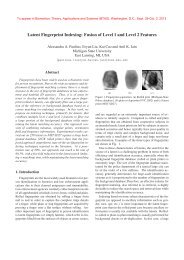
(a) Simple Frame(b) Simple Frame Classification(c) Difficult Frame(d) Difficult Frame ClassificationFigure 1.2. Background classification using only RGB featuresLocal illumination changes are more difficult to handle because if the region is recognized asforeground then it is likely to be processed by a high level tracker. This is because its shape canbe similar to other real world objects.Illumination changes may also be gradual or sharp.Gradual illumination changes can behandled by adaptive background modeling algorithms with few issues. Sharp illumination changeswill generally cause a classifier to fail for a period of time until it is able to adapt to the change.If the sharp changes occur at a high enough frequency then multimodal modeling algorithms maybe able to overcome this occurrence.Figure 1.2 shows classification on a frame with low dynamic properties, as well as a framefrom the same scene that has undergone an illumination change. After background subtraction,many false positive pixels are present in the frame with the varying illumination.While theperformance in the simple frame is acceptable, it is not for the difficult frame.3

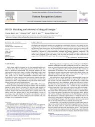
Difficulties with varying illumination conditions in background classification is one of themotivating issues for this work.Most background classification algorithms either ignore theproblem, or apply a specific heuristic to a particular domain. It is the intent of this work toexamine whether training classifiers on different image features will allow a meta-classifier to bemore robust to difficult scenarios such as illumination changes and dynamic backgrounds, whilestill handling the simple background classification scenarios. Heightened performance is desiredin general classification as well.In this work a novel solution to background classification is presented where multiple backgroundclassifiers are used. These classifiers operate on features that include the standard RGBintensities, gradient orientation, gradient magnitude, and eight separate Haar features. The resultsgenerated support the fact that this is a superior method to background classification ifcomputation demands are not considered. Using the approach described throughout the rest ofthe paper offers a promising new direction in background classification in difficult environments.In Figure 1.3, classification using the multiple classifiers algorithm presented in this paperon the same two frames that were classified using RGB features in Figure 1.2 is shown. In thedifficult frame that is undergoing an illumination change it is seen that background subtractionyields much better classification results. Performance in both frames are acceptable, which wasnot the case using only RGB features.The remainder of the thesis is organized as follows: In Chapter 2 related works to this paperare discussed. Section 2.1 discusses the early approaches to background classification, Section2.2 discusses recent methods of background classification, Section 2.3 explains work that focuseson illumination issues in background modeling, and Section 2.4 discusses ensemble methods. InChapter 3 the features that the separate classifiers use are described.Section 3.1 overviewsthe use of gradient features, Section 3.2 describes the Haar features, and Section 3.3 discussesthe use of alternate color spaces in background classification. Chapter 4 details the algorithmused for background subtraction in this paper. Section 4.1 describes the changes made to theMixture of Gaussians algorithm, and Section 4.2 discusses the method used for fusing the ensembleof classifiers. Chapter 5 contains the results from using the ensemble algorithm. Section 5.1describes the methodology for generating the comparative results, Section 5.2 discusses the datasets used, and in Section 5.3 the parameter space of the algorithm is discussed. In Section 5.44

(a) Simple Frame(b) Simple Frame Classification(c) Difficult Frame(d) Difficult Frame ClassificationFigure 1.3. Background classification using ensemble classifier5

comprehensive results using ROC graphs are provided. Chapter 6 concludes this work, whereSection 6.1 contains a summary of the work, Section 6.2 discusses future work, and Section 6.3provides final thoughts.6

CHAPTER 2RELATED WORKS2.1 Early Work in Background ModelingBecause of the computational demands that dynamic background modeling incurs, progress inthe field has mainly been over the past decade, paralleling the explosion of faster computers. Priorto the current robust models, simple background estimation was performed where the backgroundwas assumed to be static. In these schemes an algorithm similar to the one in Equation 2.1 wasused, where B(p) is the estimated background pixel value at pixel p, n is the number of framesused to build the background model, and I t (p) is the value of pixel p at time t.B(p) =n∑i=0I t (p)n(2.1)For a future frame t, pixel p is then predicted to be foreground (FG) or background (BG)based on Equation 2.2, where τ is the threshold (typically set around 50).if |I t (p) − B(p)| ≥ τ then F G else BG (2.2)The largest advantage of this technique is that it is fast and has very low memory requirementsbecause the images may be deleted after the average is calculated. The major problem with suchan algorithm is that it does not adapt to its environment, and it does not have the ability todetect dynamic background regions. The failure to adapt is eliminated if a running average istaken instead. The running average uses a learning rate α (where 0 < α < 1), and updates thebackground model with a new frame I new using Equation 2.3:B new (p) = α · I new (p) + (1 − α) · B old (p) (2.3)7

Updating the background image via Equation 2.3 offers a solution to not having an adaptivebackground. However a major problem still exists because the algorithm still relies heavily on τ.A poor selection of τ will either result in many false positives or false negatives. One solutionthat eliminates the usage of the rather arbitrary threshold τ is using a Gaussian distribution tomodel each pixel instead of merely the mean or running average, as is demonstrated in [2, 3].Because a pixel is modeled as a Gaussian distribution, foreground detection is based on a frame’scurrent pixel value against the variance.if |I t (p) − B(p)| ≥ σ · k then F G else BG (2.4)In Equation 2.4, now τ = σ · k, where k is some constant, typically around 2. Because thethreshold is directly related to the variance the equation is able to adapt to its environment.In [4] (one of the most influential papers in background modeling), Stauffer et al. first proposedmodeling the background as a combination of multiple Gaussian distributions. This algorithmis referred to the Mixture of Gaussians algorithm. Each pixel p is modeled with a group of KGaussian distributions for each of the red and green color components of p (It is assumed thatthe blue color component is ignored due to its poor reception in human vision), where K is aheuristic value generally set between the values of 3 and 5. The algorithm is first initialized,where a series of image frames are used to train each pixel by clustering the pixel’s observedtraining values into K sets using simple K-means clustering [5]. For each set k ∈ K, the mean(µ k ) and variance (σk 2 ) are computed to parameterize the corresponding Gaussian distribution.Because there are multiple distributions for a single pixel, each distribution k is initially weightedsuch that w(k) = ||k||||K||. There is a future constraint thatK∑w(k) = 1k=1which, holds initially as well.When a new image is processed for segmentation, a pixel is considered to match a particulardistribution if the pixel’s value is within 2.5 standard deviations, where 2.5 is a heuristic thatmay change based on a particular domain. So with K Gaussian distributions, and a pixel historyfor some pixel p = I t (x, y) at time t being {X 1 ...X t }, the probability of observing the pixel X t is:8

K∑P (X t ) = w t (k) · η(X t , µ k,t , Σ k,t ) (2.5)k=11η(X t , µ, Σ) =(2π) n 2 |Σ| 1 2e − 1 2 (Xt−µt)T Σ −1 (X t−µ t)where η is the Gaussian density function shown in Equation 2.6.As incoming images are processed each distribution matched is updated based on the pixel’svalue, a learning rate α, and the probability the new pixel belongs to the distribution, as seen inEquations 2.7, 2.8, and 2.9.(2.6)µ t = (1 − ρ) · µ t−1 + ρ · X t (2.7)σ 2 t = (1 − ρ) · σ 2 t−1 + ρ · (X t − µ t ) T · (X t − µ t ) (2.8)ρ = α · η(X t |µ k , σ k ) (2.9)The mean and variance of unmatched distributions remain the same.The weights of everydistribution are updated based on Equation 2.10, where M t (k) is 1 if distribution k is matchedat time t, and 0 otherwise.w t (k) = (1 − α) · w t−1 (k) + α · M t (k) (2.10)In order to determine if the pixel is a member of the background or foreground, the sum ofeach matched distribution’s weight, β, is calculated. If this value is greater than the threshold T ,then the pixel is classified as a member of the background, otherwise it is classified as foreground.The value for T is typically around 0.2.The novelty of the approach in [4] at the time it was presented greatly affected the futureprogress of background modeling. This is because by using a mixture of distributions, the algorithmcan handle dynamic background events as well as gradual illumination changes. Previousalgorithms failed to make this guarantee.The parameter space used in Mixture of Gaussians background modeling is characterizedand evaluated by Atev et al. in [6]. The effects of setting α and β, using various covariance9

epresentations, and various color spaces were explored in order to understand the effects ofaltering the parameters.In [7], Gordon et al. used a Mixture of Gaussians along with depth information from a stereovision system. Adding the depth component demonstrated more effective results in regions withmany foreground objects, but the use of this algorithm is contingent on the implementation ofa stereo vision surveillance system. Similarly, in [8], depth information generated from a stereovision system is used with a Mixture of Gaussians model by Harville. In this method Harville etal. use YUV color space in order to make the algorithm more illumination invariant. Also thelearning rates for each pixel are dynamic in order to allow pixels to adapt at different rates basedon the unique characteristics that the pixel observes.First proposed by Karmann et al. in [9] and later by Ridder et al. in [10], using a Kalman filter[11] to model the background is another popular method of performing background classification.A Kalman filter is a recursive estimator that makes a predication on a future state of a variablebased on previous state information and noise estimation. When used in background estimationeach image pixel is modeled with a Kalman filter. A key advatage of a Kalman filter is its abilityto handle slow illumination changes. Because it recursively updates itself and accounts for noise inthe estimations, slow illumination changes are seamlessly incorporated into the filter. The failingsin a Kalman filter approach to FG/BG segmentation is its ability to handle sharp illuminationchanges. The problem is that in order to handle sharp illumination changes one must increasethe gain on the filter, because increasing the gain allows for a more rapid update. According to[10], when the gain is increased it is not possible to stop foreground objects from being rapidlyadapted to by the filter and becoming modeled as background. So the Kalman filter alone hasno ability to distinguish between sharp background changes and foreground objects.Based on the equations used in [9] and [10], the procedure for using a Kalman filter inbackground modeling is as follows. A pixel p is classified as foreground if |I(p)−ŝ t (p)| > τ, whereτ is the threshold and ŝ t is the Kalman filter prediction at time t. ŝ t is generated using Equations2.11, 2.12, and 2.13. Both α and β are learning rates, where α < β in order to update the filterless when a foreground outlier is present.10

ŝ t (p) = ŝ t−1 + K(p, t) · (I t (p) − ŝ t−1 ) (2.11)K(p, t) = α · m t−1 (p) + β · (1 − m t−1 (p)) (2.12)if I i (p) = F G then m i (p) = 1 else m i (p) = 0 (2.13)When we have a small number of images for background modeling, the use of a frame differencingalgorithm is common [12]. In frame differencing, the difference between two adjacentframes is used to determine the presence of foreground, as seen in Equation 2.14. Again, the advantageof this algorithm is that it is able to operate on a limited amount of data. Shortcomingslie in the fact that the size of the detected foreground regions will be too large, large holes mayexist inside of objects, and dynamic background detection is difficult.if |I t (p) − I t−1 (p)| ≥ τ then F G else BG (2.14)Toyama et al. describe the Wallflower framework in [13], which performs background subtractionin three separate phases: at the pixel level, region level, and frame level. The pixel levelsuses a Wiener filter to predict future intensity value of the pixel. If this differs beyond a thresholdthen the pixel is considered a member of the foreground. This approach is similar to usinga Kalman filter for background classification. The region level incorporates spatial informationfrom neighboring pixels into each pixel’s classification. The frame level is used to incorporate amulti-modal property into the framework. Multiple pixel models are used to handle the differentmodes each pixel has observed. These modes are defined using K-means clustering over a trainingperiod.2.2 Modern Techniques in Background ClassificationIn [14], Zhang et al. build on the work done by Stauffer in [4], and the work by Hou and Hanin [15]. They use the same K-means clustering of adaptive Gaussians to model the background.Their technique varies in that the initialization of the Guassians is performed based on theassumption that a pixels background value will always be more frequent then a pixels foregroundvalue. Using this assumption the Gaussians are built around an initialization image set. As11

each frame is processed a pixel’s value is used to update its Mixture of Gaussians based on itssimilarity to each Gaussian.In [16], Shimada et al.propose an improvement to the Mixture of Gaussians framework,where the number of distributions may increase or decrease throughout tracking. The algorithmis highly similar to the one in by Stauffer and Grimson in [4], where the key difference is theaddition of steps that decide on whether or not to add or remove a Gaussian. A new distributionis added if no current distribution matches the current pixel value. A distribution is removedwhen its weight decreases below an heuristic threshold. Also two distributions will be combinedif the difference of their means are below a certain threshold. One of the most significant benefitsdemonstrated by this technique is improving the runtime. A direct relation was shown betweenthe computation time and the number of Gaussians. By modulating the number of distributionsan optimal number will always be used, ensuring a minimal amount of computation.A specialized Kalman filter is used by Gao et al. in [17] to model the background. Thebackground is modeled based on small regions instead of a pixel based model. This is based onthe assumption that illumination changes and noise are identical to pixels within a region. Theparameters of the Kalman filter are predicted by a recursive least square (RLS) filter. The useof a RLS filter allows for proper parameterization of the Kalman filter in various illuminationconditions.Messelodi et al. propose a Kalman filter that is able to handle sharp, global illuminationchanges in [18]. This is detected by performing a ratio comparison between each pixel to thebackground models value. For each pixel p, the value I t (p)/K(p) (where K(p) is the Kalmanpredicted value at pixel p) is placed in a histogram. If the peak of the histogram does not lienear 1 then a sharp illumination change is considered to have occurred.This approach wasdemonstrated to have highly satisfactory results in recognizing the sharp illumination changes.The major drawback of this technique is that it does not successful handle dynamic backgroundregions, such as moving leaves.In [19], Wang and Suter propose a background model using consensus methods, which essentiallystacks separate background models that each use a largely disjoint set of parameters. Inthe paper these parameters are the separate color components in RGB, though any other pixelproperty could be used instead. A three phase procedure is used to generate the background12

Segmenting images through the concept of image layers is a popular approach to binarysegmentation, where the layers represent different planes or object groups in an image Typicallymany layers will represent both the foreground and background. A foreground layer is generallyconsidered a layer that has spatiotemporal change.Criminisi et al. perform background classification using image layering in [22]. A probabilisticapproach is used where the motion, color, and contrast are combined with the spatial and temporalpriors. This use of motion cues is generally a limiting feature due to the computational demands,however the algorithm presented is able to run in real-time because the actual pixel velocities arenever computed. Instead a binary motion value is assigned to represent the presence or absenceof motion.In [23], Patwardhan et al. present an automated method of pixel layering. The algorithm has along initialization step followed by a simpler detection process. T frames are used in initialization.The first frame is segmented using the following procedure. The maximum of the histogram ofthe gray level pixel intensities, h max is found, and all pixels whose gray levels are within h max ± ρare added to the initial layer, where ρ is derived from the image covariance matrix. A samplingof the about 10-20% of the image is used to perform a Kernel Density Estimation (KDE), whichgenerates a probability density function for the initial layer based on a pixel’s feature vector (inthis case RGB features are mapped to the space presented in [24], which is discussed further inSection 2.3.). Based on the KDE probability, the image pixels are reassigned to the layer, whichis called the refinement step. The sampling and KDE continues until the initial layer stabilizes.The previously extracted layer is suppressed from the initial histogram and this process of layerextraction continues until a Kullback-Leibler divergence states the most recent extracted layerwas not meaningful. The rest of the images are processed using the previous layers and startingat the refinement step.Once the image set is layered from the initialization, future frames are able to be processed.In order to incorporate spatial information, a w × w × M window is used for each pixel, whereM is the the amount of previous frames being considered, and w is the amount of pixels in the xand y direction considered for spatial information. For each layer that exists in this window, theKDE is used to generate the probability that pixel p belongs to the layer, as well as the layer of14

outliers which comprises the foreground. Depending on the layer classification, the pixel is thenclassified as foreground or background.Optic flow [25] has been used for image segmentation as well. In [26], Zucchelli et al. clustermotion fields in order to recognize image planes. While these planes are not applied to foregroundsegmentation, the step is highly intuitive given the planes recovered. The use of motion in imagesegmentation has been gaining traction recently because of new hardware implementations thatare able to calculate flow in real-time. This represents an exciting avenue for future researchusing this additional feature.In [24], motion is used directly for background subtraction. Kernel Density Estimation [27] isused to model the distribution of the background using five dimensional feature vectors. Basedon this distribution classification is performed based on thresholded probabilities of instancesbelonging to the background distribution. The feature vectors consist of three dimensions fromcolor space intensities, and two from optic flow measurements (which consists of the flow measurementsand their uncertainties). This algorithm performed extremely well when compared toMixture of Gaussian models.2.3 Illumination ConsiderationsMany approaches have been used for illumination invariant background classification. Onereason for poor FG/BG segmentation in varying illumination is because most tracking systemsrely on color from RGB color space, which is highly variant to illumination changes. Becausegrayscale color space is a linear transformation from RGB the same problem exists. A commonsolution is the non-linear mapping of RGB color to another color space that is less illuminationinvariant.Many color conversions that claim to be illumination invariant have been proposed. Theoritically,the hue component of HSI color space and the luma commponent (Y) of YCbCr colorspace are illumination invariant, however in practice this is not typically the case (see Section3.3). In [24] Mittal and Paragios use a color mapping of RGB → rgI (where I = (R + G + B)/3,r = 3R/I, and g = 3G/I) due to claimed illumination invariance under certain conditions. Experimentationperformed in this work using this color space failed to observe such illuminationinvariant conditions, though this is not to say they do not exist. In [28], Gevers and Smeulders15

present the color space in Equation 2.15 as another illumination invariant color space. A furtherdiscussion of the observed failures using these alternate color spaces can be found in Section 3.3.l 1 =l 2 =l 3 =(R − G) 2(R − G) 2 + (R − B) 2 + (G − B) 2(R − B) 2(R − G) 2 + (R − B) 2 + (G − B) 2 (2.15)(G − B) 2(R − G) 2 + (R − B) 2 + (G − B) 2Illumination changes often cause errors in background segmentation because when illuminationchanges are sharp the pixel intesity value will vary considerably. When these changes arenot global and isolated in time, careful color space analysis is often used to prevent these illuminationchanges being improperly classified. In [29], Horprasert et al. perform segmentation intofour separate pixel classes: normal background, shaded background, highlighted background, andforeground. This is accomplished by statistically modeling each pixel based on its chromacity κ(Equation 2.18) and brightness α (Equation 2.17), where, over an observed initialization period,µ R (p) is the mean value for the red color channel at pixel p, σ G (p) is the variance over the periodfor the green color channel, and I B (p) is the current value pixel p.α p= argmax α[ (IR (p)−α p·µ R (p)) 2+(IG (p)−α p·µ G (p)σ G (p)σ R (p)()I R (p)·µ R (p)σR 2 + I G (p)·µ G (p)(p)σG 2 + I B (p)·µ B (p)(p)σ([ ] [ ] [ B 2 (p)µR (p) µG (p) µB (p)+ +σ R (p) σ G (p) σ B (p)=) 2 ( ) ]IB (p)−α + p·µ B (p) 2σ B (p)(2.16)]) (2.17)κ p =√ (IR (p)−α p·µ R (p)σ R (p)) 2+(IG (p)−α p·µ G (p)σ G (p)) 2+(IB (p)−α p·µ B (p)σ B (p)) 2(2.18)This model is best understood by considering pixel color values as a vector in a three dimensionalspace, where the red, green and blue color components are the different dimensions. Forany intensity value I(p), changing only the brightness of that color will result in a new intensityI ′ (p), where I ′ (p) = α · I(p). In other words, the new vector I ′ (p) is the same underlying coloras I(p), only its intensity has changed based on the radiance of the pixel under the illuminationcondition. If the chromacity (color) of the pixel has changed to I ′′ (p), however, then κ represents16

the shortest Euclidean distance from the value I ′′ (p) to the line that represents the vector I(p).This means the chromacity distance is based only the color of the pixel and not the illumination.When a new pixel is processed by the algorithm from [29], the distance κ and scale α arecomputed based on the expected value of the pixel from the initialization period.When κsurpasses a threshold the pixel is classified as foreground based on the fact that the color hassignificantly changed. Otherwise the pixel is labeled as normal background, shaded backgroundor illuminated background based on α.This algorithm does not update the expected valuesgenerated over the training period. This change could easily be applied where the mean andvariance of the pixels are updated using learning rates similar to the methods in [4]. The methodpresented also performs an automatic threshold selection based on histogram analysis, makingthe method non-parametric.In [30], Xu and Ellis use Mixture of Gaussian background modeling by mapping the RGB colorcomponents into a more illumination invariant color space. Denoting a RGB pixel as p RGB =< p R , p G , p B >, a mapping is performed such that p RGB → p rgb , where p rgb = < p r , p g , p b >,√and p i = p I / p 2 R + p2 G + p2 Bfor iɛ{r, g, b} and Iɛ{R, G, B}. Using this color space resulted in aclaimed higher performance when classifying background pixels in image sequences with variedillumination.One promising technique for background modeling with illumination invariance is using imagegradient information as features for background classification. One of the earliest applicationsof using gradient features for background subtraction was by Jabri et al. in [31]. In this workresults are shown using tracking on indoor image sequences. The background is simply modeledusing the mean and variance the features set (RGB and gradient magnitude).In [32], Javed et al. use a five dimensional feature set containing RGB, gradient magnitude andgradient direction for background subtraction. The RGB features are processed using a Mixtureof Gaussians algorithm, and the hypothesis is then augmented with information taken from theimage gradients. Results are shown to improve in an indoor sequence with varied illumination.17

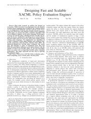
CHAPTER 3FEATURESStandard bitmaps store a three dimensional vector of features per pixel: red, green, and blueintensity values. In this work the number of features per pixels will be increased through nonlineartransformations in order to provide separate feature biases of the scenes being observed.A summary of the image features that will be used in this work can be found in Table 3.1.Using these features gives a total of 13 features per pixel. Each of these features will be used bya separate classifier that only has knowledge of its respective feature.3.1 Gradient FeaturesGradient features are used to detect edges and peaks over intensity changes in images. For thebackground classifiers, each pixel in the image frame will be characterized by the non-thresholdedvalues from the magnitude and orientation values of the Canny edge detector [44]. Using thesetwo features will offer advantages and disadvantages not found using only RGB features. A majoradvantage is found under varying illumination. In Figures 3.3(g) and 3.3(h), a comparison of thegradient magnitude of the same scene with different illumination conditions shows that gradientmagnitude remains largely invariant to the illumination change. This property will allow ourclassifier to be more robust to varying illumination conditions.One disadvantage of using the gradient magnitude is that foreground objects with homogeneousintensities will not appear to change for the classifier in the inner areas of the object. Thisfact leads to a important point about the features being used. Individually, these features do notoffer a significant enough representation of the scene for a classifier to make accurate predictions.Instead, the combination each of these lesser tracking features are assumed to provide a higherrepresentation of the image space when used in an ensemble.20

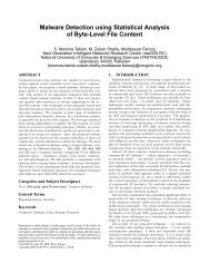
Figure 3.1. Set of Haar features being usedFigure 3.2. Illustration of equation to compute Haar valuethe value of a box is computed using Equation 3.3, which is illustrated in Figure 3.2. In theillustration, the points represent different values of the integral image. A HaarBox is any of theblack and white regions within the Haar features shown in Figure 3.1.IN(p x,y ) = IN(p x,y−1 ) + IN(p x−1,y ) − IN(p x−1,y−1 ) − I(p x,y ) (3.2)HaarBox = IN(x, y) + IN(x + width, y + height) − IN(x, y + height) + IN(x + width, y) (3.3)An example of how the value for a particular Haar feature is computed will now be shown.Suppose that Haar Feature 1 is to be computed at point x = 20, y = 20, using a 12x12 sizedwindow. First the values of the boxes that define the feature are computed. As seen in Figure3.1, one box covers the left half of the window and the other box covers the right half. For boxon the left half the boundaries of the box are: left = 14, right = 20, top = 14,bottom = 26. Forthe box on the right half the boundaries of the box are: left = 20, right = 26, top = 14,bottom= 26. Using the integral image from Equation 3.2, the value for the left box (V l ) is computedusing Equation 3.3: V l = IN(20, 26) + IN(14, 14) − IN(14, 26) − IN(20, 14). The value of the right22

ox (V r ) is: V r = IN(26, 26) + IN(20, 14) − IN(20, 26) − IN(26, 14). So the value of Haar Feature1 at point x = 20, y = 20 will be V l − V r .3.3 Alternate Color SpacesIt is common in tracking algorithms for alternate color spaces to be used, generally due totheir claimed illumination invariance.This work does not plan to use alternate color spaces,such as those mentioned in Section 2.3, primarily because illumination invariance has not beenobserved using alternate color spaces.In [28], an evaluation of various color spaces is performed to determine which are invariantto illumination changes. In this paper it is claimed that hue is invariant to illumination changes,however the images in Figures 3.3(c) and 3.3(d) show that this is not necessarily the case. Becausehue is represented as an angle θ : θ ∈ [0, 360), each pixel p in the two hue images in Figures 3.3(c)and 3.3(d) maps θ to p according to Equation 3.4. Of course, in this representation values forθ = 0 and θ = 355 will have two highly different pixel values, when the circumferal distanceis very small. However, for the purposes of this visualization that inaccuracy does no matterbecause the change in hue from the illumination change is clearly not because of this. Figures3.3(e) and 3.3(f) show that the luminance component of YCbCr also exhibits significant changesunder varying illumination.p θ = 255 ∗θ360(3.4)23

(a) Original Image, no shadow(b) Original Image, shadow(c) Hue Image, no shadow(d) Hue Image, shadow(e) Luma from YCbCr, no shadow(f) Luma from YCbCr, shadow(g) Gradient Magnitude, no shadow(h) Gradient Magnitude, shadowFigure 3.3. Effects of varying illumination on different features24

Figure 4.1. High level few of ensemble algorithm26

of distributions observed exceeds K then a behavior similar to trashing in operating systems willoccur.In this work each pixel begins with one distribution. When an new value occurs that doesnot a match a distribution, a new Gaussian is created and added to that pixel. Periodically theweight of the distributions at each pixel are checked, and distributions are removed if their weightis less than the learning rate α.Using a variable number of distributions per pixel allows each pixel to characterize the multimodalityof its observed region based on observations and not a predefined heuristic value. Thecomputational overhead is minimal when each pixel stores its distributions in a linked list.4.1.2 TrainingIn order initialize the Gaussian distributions used in the Mixture of Gaussians algorithma series of training frames are used to provide an initial characterization of the scene.Thisgenerally requires clustering the observed values from each cluster into K distributions. Unless aconvergence of clusters occurs rapidly, clustering is computationally expensive - which means themodel may not be trained in real-time. A further problem to the standard initialization is thatif a pixel’s observed training values are from a region that remained static through the trainingframes (i.e. only one cluster actually exists), that pixel’s values will still be partitioned into Kclusters.The training method for the Mixture of Gaussians algorithm in this work is a more simplifiedapproach that is enabled by the fact that the number of Gaussian distributions used is variable.Using a smaller number of training frames (less than 25), the mean of each of these pixels arecalculated and a single distribution is created for that pixel using the mean calculated and a fixedvariance, typically around 10 2 (a fixed variance is used because of regions that may have changesin their training data, causing an abnormally high variance). For static regions this approachis more robust in terms of initial accuracy and speed. For regions that observe change over thetraining frames the speed of this approach outweighs the initial lack of accuracy.One reason this approach works is that Mixture of Gaussians is an adaptive algorithm. Initiallysetting only one distribution for a pixel does not have a long term impact because as othermodes present themselves to that pixel new distributions will be added. Because the mean and27

variance are able to adapt, an initial mean and variance that are inaccurate will become correctedafter a short period of frames.4.2 Classifier FusionAs each frame is processed, and each classifier makes its predication as to whether each pixelis a member of the background or foreground, those predications must be merged into a singleprediction. Because this algorithm is an unsupervised learner, i.e. there is no labeled trainingdata or user feedback, traditional ensemble algorithms such as bagging and boosting are notpossible. Instead classifier fusion approaches will be used.Three main fusion techniques will be considered in this work, both taken from [40],[41]. Theseare the max rule, the average rule, and the majority vote rule. In [41] it was shown that for binaryclassification the max rule classifier combination is the same as the min rule, and that majorityvote is the same as median rule, which is why they are not being directly considered.If K classifiers exist, then (because P (F G) = 1−P (BG) for the two classes) the meta decisionrules are found in Equation 4.1 for the max rule, Equation 4.2 for the average rule, and Equation4.3 for the majority voite rule. In the equations, C i is the ith classifier in the ensemble, andP (BG|C i ) is the background probability predicted by classifier i. In Equation 4.3, the output ofF i (x) is 0 if P (x|C i ) < .5, and 1 if P (x|C i ) >= .5, where x ∈ BG,FG.[argmax argmaxx∈{BG,FG} i[K∑argmaxx∈{BG,FG}1Kargmaxx∈{BG,FG}i=0](P (x|C i ))P (x|C i )[∑ K]F i (x)i=0](4.1)(4.2)(4.3)It is important to note that the use of max rule combination and median rule combination arepossible because the classifiers being used are able to generate probabilities of class membership.This is because their decisions are both based on thresholding functional outputs which representa degree of membership. Contrarily, if a classifier only generated a binary decision then majorityvote would be required.28

In both [40] and [41], the average rule was shown to be the most effective fusion technique.Basic observations yield no key differences between the three when fusing the classifiers in thiswork. Because of this the average rule was used for classifier fusion in this work.29

CHAPTER 5RESULTS5.1 MethodologyIn order to evaluate the results of the proposed meta-classifier, a comprehensive method ofcomparing the outputs from the classifiers must be used.Each classifier outputs a per pixelhypothesis indicating whether that pixel is a member of the foreground or some backgroundprocess. A high level tracking system would receive these pixels, cluster them into blobs, andprocess them for a higher level semantic.Classifiers in this work will be evaluated based on their ratio of true positive to false positiveclassification. Using these measurements allows for a receiver operating characteristics (ROC)graph.ROC graphs are highly expressive, and provide a visualizable comparison of multipleclassifiers’ performances. ROC graphs are more ideal with classifiers that generate a class probabilityor degree of membership [49], which the Mixture of Gaussians does by varying the βthreshold parameter. Another benefit of using ROC graphs is that the results are invariant tothe distributions of classes [49], which is not the case using metrics such as precision and recall[50].In one method of evaluating the classifier true positive results would be based on its per pixelaccuracy, however some problems exist using this method. One major problem with a per pixelevaluation criteria is that the true positive results may be misleading. Consider, for example, ascene with two foreground objects x and y that each occupy the same number of image pixels. IfClassifier A correctly classifies all the pixels of object x as foreground and incorrectly classifies allthe pixels of object y as background, then it will have 50% true positive rate for that frame. IfClassifier B correctly classifies half of the pixels in both objects then it too will have a 50% truepositive rate. However, a strong argument could be made that Classifier B is more successful.This is due to the fact that half of an object’s pixels being classified as foreground should beenough for the higher level tracking algorithm to recognize both of these objects. The output30

from Classifier A will certainly not be sufficient in recognizing both objects. In addition to thisdrawback, generating per pixel ground truth information is highly tedious and prone to error.Another method of generating true positive results is based on the number of objects correctlyfound, which is the method that will be used in this work. Using this method the ground truthwill consist of bounding box locations of the foreground objects. Because the bounding box foreach foreground object will also contain background pixels, whether or not an object is found willbe based on the percentage of pixels classified as foreground within the box.There are few choices for representations of false positives. These pixels could be grouped intoobjects and the number of false objects found would then be reported, however this metric failsto incorporate the size or shape of the objects found. Instead, a simple count of the number offalse positive pixels will be used. Of course, this will only include pixels outside of the boundingbox, ground truth regions labeled as foreground. The ROC graphs presented will list the amountof false positives in a range of 0 to 1. This will be the average number of false positives pixelsfrom each frame divided by the total area of the frame. Of course this prevents ever having thefalse positive ratio equal 1 when foreground objects are present because not all pixels can belabeled as false positive. The alternative is represent the number the false positives in a frame asthe number of false positive pixels divided by the amount of possible false positive pixels (whichwould be the total image area minus the area occupied by foreground regions). Theoretically thisis the appropriate metric, however is has the potential to falsely characterize the performance.The reason for this is that is that the false positive measure will be a function of the foregroundsize. If one frame has a low number of foreground regions then the a small number of false positivepixels will appear equally as negative as a frame with a large number of foreground regions andmany more false positive pixels. Clearly the false positive performance in the later case is worseand should be reflected when analyzing the total results over a feature set.5.2 Data SetsThree publicly available data sets are used in this work for evaluation. Two of the data sets aretaken from the International Workshop on Performance Evaluation of Tracking and Surveillance(PETS). One is data set 2 from the 2001 conference [51], and the other is from data set S3, subset31

Table 5.1. Description of data sets usedData Set Setting Difficulty Resolution Frame Rate IlluminationOTCBVS[52] Outdoor Hard 320 x 240 Low Highly DynamicPETS 2001 [51] Outdoor Medium 768 x 576 High Slightly DynamicPETS 2006[53] Indoor Easy 720 x 576 High StaticFigure 5.1. Sample frames from OTCBVS data set3, from the 2006 conference. The third data set used is data set 03 from the OTCBVS dataset[52]. These sets each represent separate image domains as seen in Table 5.1.The OTCBVS data set offers the most difficultly due to the varying illumination caused fromcloud cover. The examples that were shown in Figure 3.3 were taken from this data set. Thesharp illumination changes caused from rolling cloud cover causes extreme variations in the RGBintensities and do not match the background distributions in the Mixture of Gaussians model.More sample frames from the OTCBVS data may been seen in Figure 5.1.As will be mentioned in Section 5.3, each data set is split into two separate sets: one fortraining to generate the optimal parameters, and one for testing. The split of the PETS 2001data sets was such that in the training set no major illumination variations were present andin the testing set a gradual, global illumination change occurred.This non-stratified split isexpected when performing sequential splits of data sets, but it causes a suboptimal performanceof all classifiers tested on the test set. One solution would be to generate the split of the testingand training sets by putting every other image in one set because this would reflect the sameillumination condition in each set. This was not done, however, because having unpredictableconditions in an image set demonstrates a greater reflection of the real world difficulties trackingsystems face.32

Figure 5.2. Sample frames from PETS 2001 data setFigure 5.3. Sample frames from PETS 2006 data setOther than the global illumination change at the end of the PETS 2001 data set it is not aterribly difficult data set. There are trees which sway lightly from wind and some foregroundobjects that are off far in the distance. Figure 5.2 contains sample images from the PETS 2001data set.The PETS 2006 data set is the easiest data set of the three. It is in an indoor environment andthe camera is in close proximity to the foreground objects. The largest difficultly is the reflectanceof the floor which causes minor reflections from the foreground objects. Sample frames from thePETS 2006 data set may be found in Figure 5.3.5.3 Parameter SelectionEach of the three data sets were separated into two dichotomic, sequential sets, where onewas used for training/parameter exploration, and the other was used for evaluation. Tables 5.2and 5.3 show the precise splits that were used for each data set. Three parameters exist in the33

Table 5.2. Frames used for trainingData Set Training Frames CountOTCBVS Subset 1b: ”img 00000.bmp” - ”img 02106.bmp” 1054PETS 2001 Subset Camera 1: ”0001.jpg” - ”2989.jpg” 2989PETS 2006 ”S7-T6-B.00000.jpg” - ”S7-T6-B.01700.jpg” 1701Table 5.3. Frames used for testingData Set Testing Frames CountOTCBVS Subset 2b: img 00000.bmp - img 01200.bmp 601PETS 2001 Subset Camera 2: ”0001.jpg” - ”2989.jpg” 2989PETS 2006 ”S7-T6-B.01701.jpg” - ”S7-T6-B.03400.jpg” 1700Mixture of Gaussians algorithm. The first parameter is the learning rate α of the classifier. Theoptimality of this parameter is largely dependent on the frame rate of the image sequence. Thenext parameter is the scale factor of the standard deviation for matching an incoming value toan existing distribution, which we will refer to as k. In [4], k was set to 2.5.The final parameter is the threshold β, which is the parameter that determines what the totalweight of the matched Gaussian distributions at a pixel must be for an object to be background.This parameter is varied in order to generate a ROC graph so its optimality was not explored.An example of the effects of varying this parameter on a classifier’s hypothesis over an imageis shown in Figure 5.4. The raw image in Figure 5.4(b) shows the classifier predictions prior tothresholding. The sum of matched weights for each distribution at a pixel is multiplied by 255 inorder to map a range of [0, 1] to [0, 255], where the closer to 0 (black) a pixel is the more likelyit is background and the closer to 255 (white) a pixel is the more likely that pixel is foreground.ROC graphs were generated for a discrete sampling of α and k, whereα ∈ {.001, .0025, .005, .01, .02, .04} and k ∈ {1.5, 2.5, 3.5, 4.5}. This resulted in 24 distinct parametercombinations tested for each data set using the traditional RGB feature set. Table 5.4 liststhe parameters selected for each data set based on these evaluations.Table 5.4. Parameters used for each data setData Set α kOTCBVS [52] .0025 2.5PETS 2001 [51] .001 1.5PETS 2006 [53] .001 1.534

(a) Original Image(b) Non-Thresholded Classifier Hypothesis Image(c) Threshold=130(d) Threshold=170(e) Threshold=210(f) Threshold=250Figure 5.4. Example of thresholding a classifier hypothesis35

The ground truth for the test sets were taken at about every 30 frames in the set, startingabout 800 to 1000 frames into the set.This offered a representation of the entire set whileprovided enough time for the classifier to stabilize after initialization.5.4 ResultsThe overall results for using the presented feature sets are extremely encouraging. The use ofthe extended feature set outperformed the baseline RGB classifier all three data sets. The mostsignificant gains were observed in the OTCBVS data set and the PETS 2001 data set. Each ofthese are outdoor data sets and present different illumination issues. Performance in the PETS2006 data set was also slightly improved, but because the data set itself is not difficult onlylimited gains were possible.When evaluating the results of ensemble classifiers in the ROC graphs, five separate featurecombinations will be compared. The first set of features compared is the performance using onlythe RGB features. This is the baseline performance and failure to improve upon classificationusing only RGB features implies an overall failure of the feature set. The second set of featuresbeing compared is the use of every feature mentioned in this paper, which will be referred to asthe extended feature set. This is 13 features (3 for RGB, 2 for gradient, and 8 for Haar). Thenext two feature sets compared are only the Haar features and only the gradient features. Finallya feature set with only the RGB and gradient features is compared.5.4.1 OTCBVS Data SetIn Figure 5.10 the ROC graph of the performance for each feature set on the OTCBVS dataset is shown. The performance of classification using only the RGB features is clearly the worst.Using all of the features appears to perform the best unless a liberal acceptance of false positivesis used, in which case it only performs slightly worse than then using only the Haar features.The OTCBVS data set is the most difficult data set because of the trouble the cloud covercauses. Difficulties in classification on this data set was largely responsible for the concept ofusing an extended feature set. The overwhelmingly higher performance of the extended featureset compared to the RGB feature set is viewed a major success.36

In Figure 5.6, an ROC graph of the performance of classifiers using only individual featuresis shown. The results show that the individual features that make up the extended feature set donot perform well individually. This is especially the case with the Haar features which generatea high number of false positives when working independently. These results are expected fromthe individual classifiers that make up an ensemble. That is, a successful ensemble classifier isgenerally the fusion of many weak classifiers [34]. Though the gradient magnitude outperformsthe baseline RGB, this will be shown to not be consistent throughout all the data sets. Furtheranaylsis of the individual features performance will be shown for the other data sets and discussedin Section 5.4.4.Results of the false alarm rate at a 90% true positive rate for each frame tested are shown inFigure 5.7. The performance of using all features is highly consistent, while when using the RGBfeatures results more sporadic, and worse at every frame. Consistency in classification is a highlydesirable feature, and it is clearly exhibited here when using the extended feature set.Sample bitmaps of the classification of a frame in the OTCBVS data set at various thresholdsare shown for RGB classification in Figure 5.8 and classification using the entire feature set inFigure 5.9. The dramatic effects of the cloud cover is apparent in both, but it is significantlydiminished using the extended feature set. In the RGB classification using a more discriminatingthreshold erodes the foreground objects before eroding the erroneous classification of the cloudcover, as clearly visible in Figure 5.8. Observing the bitmaps from the extended feature set showthat while optimal performance is still not achieved, the gains are clear and significant whencompared to using the RGB feature set.5.4.2 PETS 2001 Data SetThe results for the PETS 2001 data set are shown in Figure 5.10. It is quite clear that thebaseline RGB feature set was easily beaten by all other combinations. Once again using all 13features generated the optimal performance throughout most of the ROC graph. Depending onthe accepted tolerance for false positives, using only the Haar features and only the gradientfeatures offer solid performance as well.The disparity between the performance of the traditional RGB feature set’s performance andthe extended feature set’s performance are clear and significant when classifying on the PETS37

1OTCBVS - Total Performance0.90.80.7True Positives0.60.50.40.30.20.1RGBRGB and GradientAll FeaturesGradientHaar0 0.05 0.1 0.15 0.2False PostivesFigure 5.5. Overall results on the OTCBVS dataset1OTCBVS - Total Performance for Individual Features0.90.80.7True Positives0.60.50.40.30.2GrayRGBGradient MagnitudeGradient OrientationHaar 1Haar 2Haar 3Haar 4Haar 5Haar 6Haar 7Haar 80.05 0.1 0.15 0.2 0.25 0.3 0.35 0.4False PostivesFigure 5.6. Results for each individual feature on the OTCBVS dataset38

0.25All FeaturesRGBFrame-by-Frame Performance - OTCBVS0.2False Positives0.150.10.0500 2 4 6 8 10 12 14 16Figure 5.7. Frame by frame false positive results on OTCBVS dataset(a) Original Image(b) Threshold=220(c) Threshold=230(d) Threshold=240Figure 5.8. RGB classification image of an OTCBVS frame39

(a) Original Image (b) All Features, Threshold = 220(c) All Features, Threshold = 230 (d) All Features, Threshold = 240Figure 5.9. Ensemble classification image of an OTCBVS frame40

2001 data set. The same dramatic improvement was shown as well for the OTCBVS data set.This can lead to a generalization that using the extended feature set on outdoor imagery isoptimal to using only RGB features.The results of the individual features on the PETS 2001 data set are shown in Figure 5.10.Once again the individual features do not perform as well as the RGB feature set even thoughthe ensemble of these features greatly outperforms the RGB only classifier. As was also the casein the OTCBVS data set, the gradient magnitude feature does perform better than the RGBfeature. The reason for this will be discussed in Section 5.4.4.The individual frame performance is shown in Figure 5.12.Once again, using the entirefeature set results in an extremely consistent false alarm rate. This is still not the case for theRGB feature classification. It exhibits results comparable to the extended feature set initially,but this performance deteriorates significantly at the end of the data set. The end of the dataset is when the global illumination change occurs.As mentioned previously, one characteristic of the PETS 2001 data set is that there is agradual, global illumination change towards the end of the sequence. This illumination changecauses problems using only RGB features but not when using the extended feature set.Anexample of this is shown in Figures 5.13 and 5.14, where the regions in the yellow box indicatethe foreground objects, which are two people walking together.In Figure 5.13,the RGB classification of the sample frame from when the illumination changeis occurring shows that the reflectiveness of the building is causing many pixels of the building tobe classified a foreground when a more liberal threshold is applied. As that threshold is raised,though, the actual foreground pixels are lost. This shows that an optimal threshold does not existthat can discriminate the false positives from the true positives. In Figure 5.14 the same sample ispresented but classification is now done with the entire feature set. With a liberal threshold falsepositives exist as well, however as this threshold is raised the false positive regions are suppressedand the actual foreground objects are still maintained. Clearly this is an significant improvement.5.4.3 PETS 2006 Data SetFigure 5.15 contains the ROC graph for the performance of the feature sets on the PETS2006 data set. It is not the case that the RGB feature performed the worst in this set. In fact the41

PETS 2001 - Total Performance10.90.8True Positives0.70.60.5RGBRGB and GradientAll FeaturesGradientHaar0 0.002 0.004 0.006 0.008 0.01 0.012False PositivesFigure 5.10. Overall results on the PETS 2001 datasetPETS 2001 - Total Performance for Individual Features10.90.8True Positives0.70.60.50.4GrayRGBGradient MagnitudeGradient OrientationHaar 1Haar 2Haar 3Haar 4Haar 5Haar 6Haar 7Haar 80 0.01 0.02 0.03 0.04 0.05False PositivesFigure 5.11. Results for each individual feature on the PETS 2001 dataset42

0.06All FeaturesRGBFrame-by-Frame Performance - PETS 20010.050.04False Positives0.030.020.0100 5 10 15 20Figure 5.12. Frame by frame false positive results on PETS 2001 datasetperformance of the RGB feature set was quite competitive with the extended feature set. It is stillthe case, though, that the extended feature set provided the optimal performance with respectto the other feature set combinations. The poor performance when using only the Haar featuresand only the gradient features are quite notable as well. Despite the disappointing performanceof these features they still manage to augment the RGB features and make the extended featureset the optimal classifier.In Figure 5.16, the results of the individual features classification on the PETS 2006 data setare shown. The RGB clearly outperforms all other features, including the gradient magnitude.This finalizes the trend seen now in all three data sets that the individual features do not offerany consistent improvement over the RGB feature set, while using all of these features in anensemble classifier outperforms the RGB features every time.Figure 5.17 contains the performance at individual frames for the PETS 2006 data set. Theextended feature set appears less consistent in the data set.This may be rather misleading,however, because the false alarm rate is so low that the inconsistencies become exaggerated.The PETS 2006 data set offered the lowest performance gains when comparing the extendedfeature set the RGB features. The primary reason for this is that this data set is not a terribly43

(a) Original Image(b) Threshold=220(c) Threshold=230(d) Threshold=240Figure 5.13. RGB classification image of a PETS 2001 frame44

(a) Original Image(b) All Features, Threshold = 220(c) All Features, Threshold = 230(d) All Features, Threshold = 240Figure 5.14. Ensemble classification image of a PETS 2001 frame45

PETS 2006 - Total Performance10.950.90.85True Positives0.80.750.70.650.6RGBRGB and GradientAll FeaturesGradientHaar0.005 0.01 0.015 0.02 0.025False PostivesFigure 5.15. Overall results on the PETS 2006 datasetdifficult data set. Because it is an indoor environment and the foreground objects are in closeproximity to the camera there is little room for improvement from the standard RGB features.Despite this a slight improvement was still seen when incorporating gradient features and Haarfeatures. In real world use it would be unlikely to use these additional features, however, due tothe increased computational load they incur and the marginal gains they offer.5.4.4 Feature PerformanceThe performance of classifiers only using a single feature from the extended feature set waspoor, as observed in Figures 5.6, 5.11, and 5.16. When these weak classifiers are combined intoan ensemble of classifiers, the meta-classification offers substantial results. This adheres to thetheory of ensemble learning presented by Schapire in [34].An example of how a series of weak classifier hypotheses are able to result in a strong hypothesisin background classification is shown in Figure 5.18, where the 8 hypotheses from eachindividual Haar feature are shown as well as the fusion of those classifiers. The Haar classifierclearly has a tendency to over classify pixels are foreground, resulting in many false positives.This is evidenced in the ROC graphs where the classifiers using individual Haar features will bothmaximize the true positives and false positives. Fortunately there is a low overlap between these46

PETS 2006 - Total Performance for Individual Features10.90.80.7True Positives0.60.5GrayRGB0.4Gradient MagnitudeGradient OrientationHaar 10.3Haar 2Haar 3Haar 40.2Haar 5Haar 6Haar 7Haar 80.10 0.005 0.01 0.015 0.02 0.025 0.03 0.035 0.04 0.045False PostivesFigure 5.16. Results for each individual feature on the PETS 2006 dataset0.012Frame-by-Frame Performance - PETS 2006All FeaturesRGB0.010.008False Positives0.0060.0040.00200 2 4 6 8 10 12 14 16 18 20Figure 5.17. Frame by frame false positive results on PETS 2006 dataset47

features false positives and a high overlap in their true positives, resulting in strong backgroundclassification.It was observed in the PETS 2001 data set and the OTCBVS data set that the performanceof classification using only the gradient magnitude feature was more successful than using thebaseline RGB. Similar results were not observed in the PETS 2006 data set. It is believed thatthe reason this occured is that the foreground objects in the PETS 2001 and OTCBVS datasets are much farther from the camera than they are in the PETS 2006 data set. This resultsin lower resolutions for the foreground objects, which in turn implies less homogeneous regionsover the space occupied by the foreground object. The final implication is that edge featuresare more prominent on the low resolution objects. This may be observed in Figure 5.19, wherean object from the PETS 2006 and OTCBVS data set are shown as well as their correspondinggradient magnitude image. In the low resolution object it has distinct edge features over its entiresilhouette, while in the high resolution object these features are only prominent on the boundariesof the object and not in the homogeneous regions. A conclusion from this observation is thatthe use of gradient magnitude in background classification of smaller objects, or objects are fardistances, is superior to the RGB features.Due to the heightened performance of the gradient magnitude in the PETS 2001 and OTCBVSdata sets, a comparison of the performance against the extended feature set was performed. TheROC comparisons can be seen in Figure 5.20. In the OTCBVS data set, the use of all featuresresults in far more accurate classification than only using the gradient magnitude. The extendedfeature set also outperforms the gradient magnitude in the PETS 2001 data set, though thereis less significant of an improvement. Because of the consistent outperformance of the extendedfeature set over using only the gradient magnitude, it recomended to use all the features for moreaccurate classification.If computational demands are a limitation in a system observing lowresolution objects then using only the gradient magnitude is an adequate alternative.48

(a) Original Image(b) Haar 1 Classification(c) Haar 2 Classification(d) Haar 3 Classification(e) Haar 4 Classification(f) Haar 5 Classification(g) Haar 6 Classification(h) Haar 7 Classification(i) Haar 8 Classification(j) All Haar Classifications CombinedFigure 5.18. Weak hypotheses fused into a single strong hypothesis49

(a) PETS 2006 Original Image(b) PETS 2006 Magnitude Image(c) OTCBVS Original Image (4xZoom)(d) OTCBVS Magnitude Image (4xZoom)Figure 5.19. Effect of object size on gradient magnitude50

1OTCBVS - Total Performance0.90.80.7True Positives0.60.50.40.30.2All FeaturesGradient Magnitude0 0.01 0.02 0.03 0.04 0.05 0.06 0.07False Positives1PETS 2001 - Total Performance0.90.80.7True Positives0.60.50.40.30.2All FeaturesGradient Magnitude0 0.001 0.002 0.003 0.004 0.005 0.006False PositivesFigure 5.20. Classification using ensemble and gradient magnitude51

CHAPTER 6CONCLUSION6.1 SummaryTraditional image features in background classification are insufficient in many environments.Particularly outdoor environments, environments with varying illumination, and scenes where theforeground objects are either small or a far distance from the camera. Without the availabilityof additional spectral data (such as infrared or thermal), alternate feature sets will need to bederived from the standard RGB features. Using a feature set that includes gradient magnitude,gradient orientation, and eight separate Haar features for classification yielded significantly superiorclassification performance on more difficult data sets, and still marginally outperformed ina simpler data set.A summary of the performances in terms of false positive rates on all three data sets areshown in Figure 6.1 (NOTE: In Figure 6.1, false positive performance in the OTCBVS data setscaled down by a factor of 6.75). Each performance is based on the lowest false positive ratethat generated at least a 90% true positive classification rate. Table 6.1 shows the same results,as well as the ratio of improvement seen using the extended feature set.It can be seen thatfalse positives are more than 5 times higher in the OTCBVS data set, and more than 6 timeshigher in the PETS 2001 data set when using RGB features instead of the extended feature setpresented. These two data sets are both outdoor data sets with dynamic illumination events. InFigure 6.2 and Figure 6.3 ROC graphs are shown that compare RGB classification strictly to theclassification using the extended feature set on each of these two datasets.Table 6.1. False positives at a 90% true positive rateData Set RGB FP All Features FP FP RatioOTCBVS 0.1046 0.0204 5.17:1PETS 2001 0.0094 0.0014 6.71:1PETS 2006 0.0027 0.0019 1.42:152

Figure 6.1. False positive results at 90% true positive rateOTCBVS - Summary10.90.8True Positives0.70.60.50.4RGBAll Features0 0.02 0.04 0.06 0.08 0.1 0.12 0.14 0.16 0.18Figure 6.2. OTCBVS ROC graph summary53

OTCBVS - Summary10.90.8True Positives0.70.60.50.4RGBAll Features0 0.02 0.04 0.06 0.08 0.1 0.12 0.14 0.16 0.18Figure 6.3. PETS 2001 ROC graph summaryComparisons using ROC graphs clearly showed the advantage of using additional features forbackground classification in image sequences. The algorithm used was an ensemble algorithm.It fused the result of multiple classifier hypotheses into a single hypothesis.Each individualclassifier operated on only one of the features in the feature set, yielding a decision independentof all other features (assuming the features themselves are independent, which strictly speakingthey are not).Various feature set combinations were explored and the overall result was that using all of thefeatures resulted in the highest performance. Individually most features performed poorly. Thisadhered to the predominant theory in ensemble classifiers that the fusion of many weak classifierswill act together as a single strong classifier. When these features were all fused together, theclassification at a fixed true positive rate always yielded less false positives than using only RGBfeatures.One single feature that did perform well individually on two of three data sets was the gradientmagnitude. Each of the two data sets it excelled in were outdoor and the foreground objects wereat a far distance from the camera. The performance did not surpass using all of the features, butit did surpass using the RGB features. This draws the conclusion that for a low cost and more54

efficient classifier when being restricted to low resolution images of the objects being tracked,using gradient magnitude as a single feature will offer satisfactory performance gains over RGBfeatures.6.2 Future WorkThe optimistic results generated opens the door for many avenues of future research in usingensembles of background classifiers.While significant improvements were shown using Haar features, as well as gradient features,incorporating additional image processing features may allow for a further improvement. Onefeature that would be intuitive to incorporate is texture. Per pixel texture features using Gaborfilters as described in [54], [55] would offer a similar, but distinctly different, representation ofa pixel than Haar features.Additional features that could be included are the Laplacian ofGaussian, non-thresholded SIFT features [56], depth, and motion features.Another direction is the fusion of different classifier algorithms. For example, instead of usinga series of Mixture of Gaussian classifiers, an ensemble of Mixture of Gaussian, Kalman Filter,and other classifiers could be used. This approach was the first direction this work researched.The major stopping point was the lack of distinct classifiers for background subtraction.Insteadof fusing strong classifier algorithms, using a series of weak algorithms should offer similarimprovements to using an extended feature set.An extended feature set could also be used without having multiple classifiers. Because theMixture of Gaussians algorithm normally operates on a feature vector (where the three featuresare RGB), using the same features in this paper as a single vector for one classifier should produceunique results. It may not be the case that significantly different results are yielded with thisapproach unless a full covariance matrix is computed, which is generally not the case. Insteadit is generally the case that only the diagonal of the covariance matrix is calculated in order toreduce computational demands. Another consideration when using a vector of features insteadof an ensemble of classifiers is that if a single dimension of new instance vector does not fallwithin 2.5σ of its corresponding dimension, and every other vector dimension does, then theinstance does not match the distribution. With a larger feature set it is often the case that notevery feature matches its corresponding dimension for its feature in the model. This approach is55

also different than using an unanimous vote scheme for classifier fusion in the ensemble classifierpresented in this work. This is because if only a few features match the new instance the classifierswill update themselves based on a match in the ensemble algorithm, while for the single featurevector algorithm the update would not be based on a match unless every dimension was matched(where matching is being with 2.5σ).Evaluation of the ensemble algorithm’s performance could be performed using the VACE evaluationframework in [57]. This framework offers a more comprehensive analysis of the algorithmsrobustness, as well as a comparison against the performance of other tracking algorithms.Real-time implementation of this system would require a system with multiple processingcores and a large sized main memory, but otherwise its realization is believed to be reasonable.Enhanced engineering of the algorithms to exploit the inherent parallelism of the ensemble shouldallow for the handling of relatively high frame rates depending on the image resolution.6.3 Final ThoughtsIt is believed that further research needs to be conducted in order to further understand thegains that were observed in this work. There was a clearly demonstrated advantage to usingadditional features in background classification, even though many of these features are verypoor when used individually. Through greater investigation a more clearly defined set of optimalensemble features would allow for a more general background classification algorithm that couldhave key impacts in defense, robotics, and surveillance applications.56

REFERENCES[1] R. Jain, R. Kasturi, and B. Schunck. Machine Vision. McGraw Hill, 1995.[2] C. Wren, A. Azarbayejani, T. Darrell, and A. Pentland. Pfinder: Real-time tracking of thehuman body. IEEE Trans. Pattern Anal. Mach. Intell., 19(7):780–785, 1997.[3] D. Koller, J. Weber, and J. Malik. Robust multiple car tracking with occlusion reasoning.In ECCV (1), pages 189–196, 1994.[4] C. Stauffer and W. Grimson. Adaptive background mixture models for real-time tracking.In IEEE Conference on Computer Vision and Pattern Recognition, volume 2, 1999.[5] J. B. MacQueen. Some methods for classification and analysis of multivariate observations.In Proceedings of 5th Berkeley Symposium on Mathematical Statistics and Probability, pages281–297, 1967.[6] S. Atev, O. Masoud, and N. Papanikolopoulos. Practical mixtures of gaussians with brightnessmonitoring. In The 7th International IEEE Conference on Intelligent TransportationSystems, 2004.[7] G. Gordon, T. Darrell, M. Harville, and J. Woodfill. Background estimation and removalbased on range and color. In Image Processing, 2001. Proceedings. 2001 International Conferenceon, volume 2, pages 395–398, 2001.[8] M. Harville, G. Gordon, and J. Woodfill. Adaptive video background modeling using colorand depth. In Conference on Image Processing, pages 90–93, 2001.[9] K. Karmann, A. Brandt, and R. Gerl. Moving object segmentation based on adaptivereference images. In European Signal Processing Conf, pages 951–954, 1990.[10] C. Ridder, O. Munkelt, and H. Kirchner. Adaptive bbackground estimation and foregrounddetection using kalman filtering. In In Proc. ICAM, pages 193–199, 1995.[11] R. E. Kalman. A new approach to linear filtering and prediction problems. Journal of BasicEngineering, 82:3545, 1960.[12] M. Leung and Y. Yang. Human body motion segmentation in a complex scene. PatternRecognition, 20(1):55–64, 1987.[13] K. Toyama, J. Krumm, B. Brumitt, and B. Meyers. Wallflower: Principles and practice ofbackground maintenance. In ICCV (1), pages 255–261, 1999.[14] Y. Zhang, Z. Liang, Z. Hou, H. Wang, and M. Tan. An adaptive mixture gaussian backgroundmodel with online background reconstruction and adjustable foreground mergence time formotion segmentation. In IEEE International Conference on Industrial Technology, volume14-17, pages 23–27, 2005.57

[15] Z. Hou and C. Han. A background reconstruction algorithm based on pixel intensity classificationin remote video surveillance system. In Proceedings of the Seventh InternationalConference on Information Fusion, pages 754–759, 2004.[16] A. Shimada, D. Arita, and R. Taniguchi. Dynamic control of adaptive mixture-of-gaussiansbackground model. In Proceedings of the IEEE International Conference on Video and SignalBased Surveillance, page 5, 2006.[17] D Gao, J Zhou, and L Xin. A novel algorithm of adaptive background estimation. InInternational Conference on Image Processing, 2001.[18] S. Messelodi, C. Modena, N. Segata, and M. Zanin. A kalman filter based backgroundupdating algorithm robust to sharp illumination changes. In ICIAP 2005, 13th InternationalConference on Image Analysis and Processing, pages 163–170, 2005.[19] H. Wang and D. Suter. Background subtraction based on a robust consensus method. InICPR ’06: Proceedings of the 18th International Conference on Pattern Recognition, pages223–226, Washington, DC, USA, 2006. IEEE Computer Society.[20] S. Avidan. Ensemble tracking. IEEE Transactions on Pattern Analysis and Machine Intelligence,29(2):261–271, 2007.[21] Y. Freund and R.E. Schapire. Decision-theoretic generalization of on-line learning and anapplication to boosting. Journal of Computer and System Sciences, 55(1):119139, 1997.[22] A. Criminisi, G. Cross, A. Blake, and V. Kolmogorov. Bilayer segmentation of live video.CVPR, 1:53–60, 2006.[23] K. Patwardhan, G. Sapiro, and V. Morellas. Robust foreground segmentation using pixellayers. Pattern Analysis and Machine Intelligence, IEEE Transactions on, 4:746–751, 2008.[24] A. Mittal and N. Paragios. Motion-based background subtraction using adaptive kerneldensity estimation. Computer Vision and Pattern Recognition, 2:302–309, 2004.[25] B.K.P. Horn and B.G. Schunck. Determining optical flow. Artificial Intelligence, 17:185203,1981.[26] M. Zucchelli, J. Santos-Victor, and H. Christensen. Multiple plane segmentation using opticalflow. In British Machine Vision Conference, 2002.[27] B. W. Silverman. Density Estimation for Statistics and Data Analysis. Chapman and Hall,1986.[28] T Gevers and A Smeulders. Color-based object recognition. Pattern Recognition, 32(3):453–464, 1999.[29] T. Horprasert, D. Harwood, and L. S. Davis. A statistical approach for real-time robustbackground subtraction and shadow detection. In ICCV, 1999.[30] M. Xu and T. Ellis. Illumination-invariant motion detection using colour mixture models.In British Machine Vision Conference, 2001.[31] S. Jabri, Z. Duric, H. Wechsler, and A. Rosenfeld. Detection and location of people in videoimages using adaptive fusion of color and edge information. In International Conference onPattern Recognition, volume 4, pages 627–630, 2000.58

[32] O. Javed, K. Shafique, and M. Shah. A hierarchical approach to robust background subtractionusing color and gradient information. In Motion and Video Computing, Proceedings ofWorkshop on, pages 22–27, 2002.[33] B.V. Dasarathy and B.V. Sheela. Composite classifier system design: Concepts and methodology.Proceedings of the IEEE, 67(5):708–713, 1979.[34] R. Schapire. The strength of weak learnability. Machine Learning, 5(2):197–227, 1990.[35] L. Breiman. Bagging predictors. Machine Learning, 24(2):123140, 1996.[36] D.H. Wolpert. Stacked generalization. Neural Networks, 5:241–259, 1992.[37] R.A. Jacobs, M.I. Jordan, S.J. Nowlan, and G.E. Hinton. Adaptive mixtures of local experts.Neural Computation, 3:7987, 1991.[38] R. Polikar. Ensemble based systems in decision making. IEEE Circuits and Systems Magazine,6(3):21–45, 2006.[39] N. Siebel and S. Maybank. Fusion of multiple tracking algorithms for robust people tracking.In Proceedings of the 7th European Conference on Computer Vision, volume IV, pages 373–387, May 2002.[40] J. Kittler, M. Hatef, R. Duin, and J. Matas. On combining classifiers. Pattern Analysis andMachine Intelligence, IEEE Transactions on, 20(3):226–269, 1998.[41] L. Kuncheva. A theoretical study on six classifier strategies. Pattern Analysis and MachineIntelligence, IEEE Transactions on, 24(2):281–286, 2002.[42] T. Ho, J. Hull, and S. Srihari. Decision combination in multiple classifier systems. PatternAnalysis and Machine Intelligence, IEEE Transactions on, 16(1):66–75, 1994.[43] A. Ross and A.K. Jain. Information fusion in biometrics. Pattern Recognition Letters,24(13):2115–2125, 2003.[44] J. Canny. A computational approach to edge detection. IEEE Transactions on PatternAnalysis and Machine Intelligence, 8:679–714, 1986.[45] C. Papageorgiou, M. Oren, , and T. Poggio. A general framework for object detection. InIn International Conference on Computer Vision, 1998.[46] M. Oren, C. Papageorgiou, P. Sinha, E. Osuna, and T. Poggio. Pedestrian detection usingwavelet templates. In Proc. Computer Vision and Pattern Recognition, pages 193–199, 1997.[47] P. Viola and M. Jones. Rapid object detection using a boosted cascade of simple features.In Proceedings IEEE Conference on Computer Vision and Pattern Recognition, 2001.[48] R. Lienhart and J. Maydt. An extended set of haar-like features for rapid object detection.In International Conference on Image Processing, 2002.[49] T. Fawcett. An introduction to roc analysis. Pattern Recognition Letters, 27:861–874, 2006.[50] J. Makhoul, F. Kubala, R. Schwartz, and R. Weischedel. Performance measures for informationextraction. In Proceedings of DARPA Broadcast News Workshop, 1999.[51] PETS 2001 Dataset. ftp://ftp.pets.rdg.ac.uk/pub/PETS2001. Data set 2.59

[52] OTCBVS Benchmark Dataset Collection. http://newton.ex.ac.uk/tex/pack/bibtex/btxdoc/node6.html. Data set 03.[53] PETS 2006 Dataset. http://www.cvg.rdg.ac.uk/PETS2006/data.html. Data set S3.[54] A.K. Jain and F. Farrokhnia. Unsupervised texture segmentation using gabor filters. InSystems, Man and Cybernetics, IEEE International Conference on, 1990.[55] B. Manjunath and W. Ma. Texture features for browsing and retrieval of image data. PatternAnalysis and Machine Intelligence, 18:837–842, 1996.[56] D. Lowe. Distinctive image features from scale-invariant keypoints. International Journal ofComputer Vision, 60(2):91–110, 2004.[57] V. Manohar, M. Boonstra, V. Korzhova, P. Soundararajan, D. Goldgof, R. Kasturi,S. Prasad, H. Raju, R. Bowers, and J. Garofolo. Pets vs. vace evaluation programs: Acomparative study. In Proceedings of the Ninth IEEE International Workshop on PerformanceEvaluation of Tracking and Surveillance, 2006.60