Evaluation of the New WAAS L5 Signal - University of New Brunswick
Evaluation of the New WAAS L5 Signal - University of New Brunswick
Evaluation of the New WAAS L5 Signal - University of New Brunswick

You also want an ePaper? Increase the reach of your titles
YUMPU automatically turns print PDFs into web optimized ePapers that Google loves.
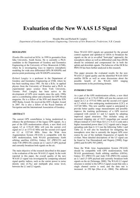
<strong>Evaluation</strong> <strong>of</strong> <strong>the</strong> <strong>New</strong> <strong>WAAS</strong> <strong>L5</strong> <strong>Signal</strong><br />
Hyunho Rho and Richard B. Langley<br />
Department <strong>of</strong> Geodesy and Geomatics Engineering, <strong>University</strong> <strong>of</strong> <strong>New</strong> <strong>Brunswick</strong>, Fredericton, N.B. Canada<br />
BIOGRAPHY<br />
Hyunho Rho received an M.Sc. in 1999 in geomatics from<br />
Inha <strong>University</strong>, South Korea. He is currently a Ph.D.<br />
candidate in <strong>the</strong> Department <strong>of</strong> Geodesy and Geomatics<br />
Engineering at <strong>the</strong> <strong>University</strong> <strong>of</strong> <strong>New</strong> <strong>Brunswick</strong> (UNB),<br />
where he is investigating ways to improve ionospheric<br />
modeling for wide area differential GPS (WADGPS) and<br />
precise point positioning with WADGPS corrections.<br />
Richard Langley is a pr<strong>of</strong>essor in <strong>the</strong> Department <strong>of</strong><br />
Geodesy and Geomatics Engineering at UNB, where he<br />
has been teaching since 1981. He has a B.Sc. in applied<br />
physics from <strong>the</strong> <strong>University</strong> <strong>of</strong> Waterloo and a Ph.D. in<br />
experimental space science from York <strong>University</strong>,<br />
Toronto. Pr<strong>of</strong>. Langley has been active in <strong>the</strong><br />
development <strong>of</strong> GPS error models since <strong>the</strong> early 1980s<br />
and is a contributing editor and columnist for GPS World<br />
magazine. He is a fellow <strong>of</strong> <strong>the</strong> ION and shared <strong>the</strong> ION<br />
2003 Burka Award. He received <strong>the</strong> ION’s Kepler Award<br />
in 2007. He is also a fellow <strong>of</strong> <strong>the</strong> Royal Institute <strong>of</strong><br />
Navigation and <strong>the</strong> International Association <strong>of</strong> Geodesy.<br />
ABSTRACT<br />
The current GPS constellation is being modernized to<br />
enhance <strong>the</strong> performance <strong>of</strong> <strong>the</strong> legacy GPS signals. As a<br />
part <strong>of</strong> <strong>the</strong> GPS modernization efforts, a new third civil<br />
signal, <strong>L5</strong> at 1176.45 MHz will join <strong>the</strong> current civil<br />
signal on L1 at 1575.42 MHz and <strong>the</strong> second civil signal<br />
on L2 at 1227.60 MHz. Since <strong>the</strong> Wide Area<br />
Augmentation System (<strong>WAAS</strong>) is compatible with <strong>the</strong><br />
GPS modernization, both <strong>WAAS</strong> geostationary Earth<br />
orbiting satellites (GEOs), Galaxy XV (PRN135) and<br />
Anik F1R (PRN138) contain an L1 and <strong>L5</strong> GPS payload<br />
and currently broadcast both signals on <strong>the</strong> air.<br />
The main objective <strong>of</strong> <strong>the</strong> research described in this paper<br />
is <strong>the</strong> evaluation <strong>of</strong> <strong>the</strong> new <strong>WAAS</strong> <strong>L5</strong> signal. In <strong>the</strong> work<br />
reported in this paper, <strong>the</strong> overall quality <strong>of</strong> <strong>the</strong> new<br />
<strong>WAAS</strong> <strong>L5</strong> signal was investigated by comparing selected<br />
signal quality indices, such as <strong>the</strong> carrier power to noise<br />
density ratio (C/N 0 ) and multipath plus noise level,<br />
between <strong>the</strong> L1 and <strong>L5</strong> signals.<br />
Since <strong>WAAS</strong> GEO signals are generated by <strong>the</strong> ground<br />
control segment and uplinked to GEOs to broadcast <strong>the</strong><br />
signals on <strong>the</strong> air (a so-called “bent-pipe” approach), <strong>the</strong><br />
ionospheric delays as well as differential code bias (DCB)<br />
should be estimated and compensated for in both <strong>the</strong><br />
uplink and downlink signals. The behavior <strong>of</strong> <strong>the</strong> DCB for<br />
PRN138 has been fur<strong>the</strong>r analyzed in this research.<br />
This paper presents <strong>the</strong> evaluated results for <strong>the</strong> new<br />
<strong>WAAS</strong> <strong>L5</strong> signal quality and <strong>the</strong> identified <strong>WAAS</strong> GEO<br />
satellite DCBs as well as some discussions about <strong>the</strong><br />
possible benefit <strong>of</strong> <strong>the</strong> <strong>WAAS</strong> GEO ranging<br />
measurements in <strong>the</strong> positioning domain.<br />
INTRODUCTION<br />
As a part <strong>of</strong> <strong>the</strong> GPS modernization efforts, a new third<br />
civil signal, <strong>L5</strong> at 1176.45 MHz will join <strong>the</strong> current civil<br />
signal on L1 at 1575.42 MHz and <strong>the</strong> second civil signal<br />
on L2 which is also undergoing modernization (L2C), at<br />
1227.60 MHz. This new satellite signal is anticipated to<br />
provide better quality range measurements and possibly<br />
improve <strong>the</strong> tracking performance <strong>of</strong> a GPS receiver<br />
compared with current L1 and L2 signals by adopting<br />
improved signal structures. This includes using an<br />
increased chipping rate <strong>of</strong> 10.23 megachips per second<br />
(Mcps) instead <strong>of</strong> 1.023 Mcps for L1 C/A (C1) code and a<br />
higher transmitted power than L1/L2 signals and a longer<br />
spreading code than L1 C1 (see <strong>the</strong> following Table 1 and<br />
Table 2). It will also be beneficial for mitigating <strong>the</strong><br />
ionospheric error that is currently <strong>the</strong> largest GPS error<br />
source by use <strong>of</strong> <strong>the</strong> multiple frequencies <strong>of</strong> signals for<br />
civilian. More detailed descriptions <strong>of</strong> <strong>the</strong> <strong>L5</strong> signal can<br />
be found in Van Dierendonck and Hegarty [2000], Enge<br />
[2003] and IS-GPS-705 [2005].<br />
Since <strong>the</strong> Wide Area Augmentation System (<strong>WAAS</strong>)<br />
should be compatible with GPS modernization, both<br />
<strong>WAAS</strong> geostationary Earth orbiting satellites (GEOs),<br />
Galaxy XV (PRN135) and Anik F1R (PRN138) contain<br />
an L1 and <strong>L5</strong> GPS payload and currently broadcast both<br />
signals on <strong>the</strong> air [Schempp, 2008]. The <strong>WAAS</strong> <strong>L5</strong> signal<br />
structure is similar to <strong>the</strong> GPS <strong>L5</strong> signal except that only a<br />
single channel carrier is used, and <strong>the</strong> data rate is<br />
increased to 250 bps [Hsu et al., 2004]. The different
signal characteristics <strong>of</strong> GPS and <strong>WAAS</strong> are illustrated in<br />
Table 1.<br />
Table 1: Characteristics <strong>of</strong> GPS <strong>L5</strong> signal vs. <strong>WAAS</strong><br />
<strong>L5</strong> [IS-GPS-200D, 2004 and IS-GPS-705, 2005]<br />
GPS/<strong>WAAS</strong><br />
GPS <strong>L5</strong> <strong>WAAS</strong> <strong>L5</strong><br />
L1<br />
Carrier<br />
Frequency<br />
1176.45 MHz 1176.45 MHz 1575.42 MHz<br />
<strong>Signal</strong> Two carrier Single carrier Two carrier<br />
Structure components: component: components:<br />
I5 and Q5<br />
P(Y) and CA<br />
ranging<br />
codes<br />
C5 ranging<br />
code<br />
/CA ranging<br />
code (<strong>WAAS</strong>)<br />
Code<br />
length<br />
(chips) 10230 10230 1023<br />
Code<br />
frequency 10.23 Mcps 10.23 Mcps 1.023 Mcps<br />
Data rate 50 bps 250 bps 50/250 bps<br />
Table 2: Received Minimal <strong>Signal</strong> Strength [IS-GPS-<br />
200D, 2004 and IS-GPS-705, 2005]<br />
SV Blocks<br />
II/IIA/IIR<br />
IIR-M/IIF<br />
IIF<br />
Channel<br />
P(Y)<br />
<strong>Signal</strong><br />
C/A or L2C<br />
L1 -161.5 dBW -158.5 dBW<br />
L2 -164.5 dBW N/A<br />
L1 -161.5dBW -158.5 dBW<br />
L2 -161.5 dBW -160.0 dBW<br />
I5<br />
Q5<br />
<strong>L5</strong> -157.9 dBW -157.9 dBW<br />
In <strong>the</strong> following sections, <strong>the</strong> <strong>WAAS</strong> differential code<br />
bias (DCB) between L1 C1 and <strong>L5</strong> code (C5) are<br />
analyzed. Since <strong>the</strong> <strong>WAAS</strong> GEO ranging signals are<br />
generated by <strong>the</strong> ground control segment and uplinked to<br />
<strong>the</strong> GEO satellites for rebroadcast [Hsu et al., 2004 and<br />
2007, Grewal, 2008], <strong>the</strong> ionospheric delays as well as its<br />
differential code bias (DCB) should be estimated and<br />
compensated for in both <strong>the</strong> uplink and downlink signals.<br />
Since ano<strong>the</strong>r important role <strong>of</strong> DCB in <strong>WAAS</strong> might be<br />
to resolve <strong>the</strong> clock referencing issue in <strong>the</strong> observables<br />
for single frequency users (like <strong>the</strong> group delay term<br />
(T GD ) for GPS L1/L2 [IS-GPS-200D]), <strong>the</strong> overall<br />
behavior <strong>of</strong> <strong>the</strong> estimated DCBs were fur<strong>the</strong>r analyzed.<br />
Finally, <strong>the</strong> possible benefit <strong>of</strong> using <strong>WAAS</strong> GEO<br />
ranging measurements in <strong>the</strong> positioning domain is also<br />
discussed.<br />
In this paper, investigations <strong>of</strong> <strong>the</strong> observation quality <strong>of</strong><br />
<strong>the</strong> <strong>WAAS</strong> <strong>L5</strong> signal are presented. Fur<strong>the</strong>rmore <strong>the</strong><br />
compiled statistics <strong>of</strong> all <strong>the</strong> compared results for <strong>the</strong><br />
selected continuous four days are presented, which may<br />
be used as a baseline for fur<strong>the</strong>r research on <strong>the</strong> <strong>WAAS</strong><br />
and future GPS <strong>L5</strong> signals.<br />
OBSERVABILITY OF <strong>L5</strong> SIGNALS AT UNB<br />
<strong>WAAS</strong> currently transmits dual-frequency, L1 and <strong>L5</strong><br />
signals on <strong>the</strong> air. At UNB, <strong>the</strong> two <strong>WAAS</strong> GEOs,<br />
PRN135 and PRN138 can be simultaneously monitored.<br />
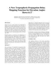
Both GEOs are located on <strong>the</strong> southwest side <strong>of</strong> UNB and<br />
PRN135 is monitored at an elevation angle <strong>of</strong> 7.6° and<br />
azimuth <strong>of</strong> 252.6°. PRN138 is monitored at an elevation<br />
angle <strong>of</strong> about 23.9° and azimuth <strong>of</strong> 230.1°. The<br />
following Figure 1 shows <strong>the</strong> observability <strong>of</strong> signals<br />
from <strong>the</strong> <strong>WAAS</strong> GEOs at UNB.<br />
A NovAtel ProPak-V3 (OEM-V3) receiver equipped with<br />
specialized firmware that allows acquisition <strong>of</strong> both L1<br />
and <strong>L5</strong> signals simultaneously from <strong>the</strong> <strong>WAAS</strong> GEOs<br />
was used to obtain test data sets at <strong>the</strong> <strong>University</strong> <strong>of</strong> <strong>New</strong><br />
<strong>Brunswick</strong> (UNB) in Fredericton Canada. A data set<br />
spanning four continuous days in August 2008 has been<br />
used to study <strong>the</strong> <strong>WAAS</strong> <strong>L5</strong> signals.<br />
This paper discusses <strong>the</strong> overall observation quality <strong>of</strong><br />
<strong>WAAS</strong> <strong>L5</strong> signals. Since <strong>the</strong> carrier power to noise<br />
density ratio (C/N 0 ) indicates <strong>the</strong> level <strong>of</strong> signal power<br />
versus <strong>the</strong> level <strong>of</strong> background noise in <strong>the</strong> observables,<br />
C/N 0 was used as a first signal quality indicator and <strong>the</strong><br />
C/N 0 values on L1 and <strong>L5</strong> signals were compared. Also<br />
<strong>the</strong> receiver tracking noise and multipath (MP)<br />
characteristics <strong>of</strong> <strong>the</strong> L1 and <strong>L5</strong> signals were compared.<br />
In this comparison, <strong>the</strong> magnitude <strong>of</strong> possible<br />
improvement from enhanced signal structures in <strong>the</strong> <strong>L5</strong><br />
signal are quantified.<br />
Figure 1. Observability <strong>of</strong> signals from <strong>WAAS</strong> GEOs<br />
at UNB
To obtain test data sets at UNB, we used a NovAtel<br />
ProPak-V3 (OEM-V3) receiver equipped with specialized<br />
firmware that allows acquisition <strong>of</strong> both L1 and <strong>L5</strong><br />
signals simultaneously from <strong>the</strong> <strong>WAAS</strong> GEOs. The first<br />
four channels <strong>of</strong> <strong>the</strong> entire sixteen-channel receiver were<br />
assigned to <strong>the</strong> two <strong>WAAS</strong> GEOs for L1 and <strong>L5</strong> dual<br />
frequency tracking and <strong>the</strong> o<strong>the</strong>r 12 channels were used<br />
for general GPS L1 and L2 dual frequency tracking. With<br />
this capability, <strong>the</strong> observation quality <strong>of</strong> <strong>the</strong> <strong>WAAS</strong> <strong>L5</strong><br />
signals could be directly compared with <strong>the</strong> <strong>WAAS</strong> L1<br />
signals and <strong>the</strong> simultaneous GPS dual frequency<br />
measurements could be used for o<strong>the</strong>r purposes such as<br />
comparing <strong>the</strong> differences <strong>of</strong> <strong>the</strong> estimated DCBs for GPS<br />
and for <strong>WAAS</strong>.<br />
Since PRN135 is seen at <strong>the</strong> low elevation angle <strong>of</strong><br />
around 7.6°, an elevation cut<strong>of</strong>f angle <strong>of</strong> 0° was used to<br />
collect data from all satellites. The collected data set for<br />
<strong>the</strong> continuous four days from 24 August 2008 to 27<br />
August 2008 have been used to assess <strong>the</strong> quality <strong>of</strong> <strong>the</strong><br />
L1 C1 and <strong>the</strong> new <strong>L5</strong> C5 code measurements<br />
(pseudoranges).<br />
METHODOLOGY<br />
The objective <strong>of</strong> this section is to describe <strong>the</strong><br />
computational methods we used to obtain “proper”<br />
observables which have been used to evaluate <strong>the</strong> <strong>WAAS</strong><br />
<strong>L5</strong> signals.<br />
Multipath Plus Noise Observables<br />
At first, pseudorange measurements can be expressed in<br />
distance units as:<br />
P = ρ + c ⋅ ( dT − dt)<br />
+ d<br />
i<br />
+ b<br />
rj,<br />
Pi<br />
+ mp<br />
Pi<br />
ion,<br />
i<br />
+ d<br />
trop<br />
+ b<br />
sk<br />
, Pi<br />
where i stands for <strong>the</strong> corresponding frequency at L1, L2<br />
or <strong>L5</strong> for satellite k and receiver j, P is <strong>the</strong> pseudorange<br />
measurement in distance units, ρ is <strong>the</strong> geometric range<br />
between <strong>the</strong> satellite and <strong>the</strong> receiver, dT and dt represent<br />
<strong>the</strong> receiver and satellite clock <strong>of</strong>fsets relative to system<br />
reference time, i.e. GPS Time for GPS satellites and<br />
<strong>WAAS</strong> network time for <strong>WAAS</strong> GEOs, d<br />
ion , i<br />
is <strong>the</strong><br />
frequency dependent ionospheric delay and d<br />
trop<br />
is <strong>the</strong><br />
s Pi<br />
tropospheric propagation delay, b , k<br />
is <strong>the</strong> satellite<br />
instrumental delay with respect to <strong>the</strong> satellite k and<br />
b<br />
rj , Pi<br />
is <strong>the</strong> receiver instrumental delays with respect to<br />
<strong>the</strong> receiver j, finally, mp<br />
Pi<br />
represents <strong>the</strong> multipath plus<br />
receiver noise in <strong>the</strong> pseudorange measurement.<br />
(1)<br />
Next, <strong>the</strong> observation equation for <strong>the</strong> carrier-phase<br />
measurement can be formed as:<br />
Φ = ρ + c ⋅ ( dT − dt)<br />
+ λ N − d<br />
i<br />
+ b<br />
sk<br />
, ϕi<br />
+ b<br />
rj,<br />
ϕi<br />
+ mp<br />
ϕ<br />
i<br />
i<br />
i<br />
ion,<br />
i<br />
+ d<br />
where<br />
( ≈ 24 cm) and <strong>L5</strong> ( ≈ 25 cm) carriers in distance units,<br />
s i<br />
N<br />
i<br />
is <strong>the</strong> carrier-phase ambiguity. b , ϕ s<br />
and brj<br />
, ϕ i<br />
represent <strong>the</strong> satellite and receiver instrumental delays on<br />
each carrier-phase observable and mp ϕ<br />
is <strong>the</strong> carrier<br />
i<br />
phase multipath and <strong>the</strong> noise.<br />
trop<br />
(2)<br />
λi<br />
is <strong>the</strong> wavelength <strong>of</strong> <strong>the</strong> L1 ( ≈ 19 cm), L2<br />
To obtain <strong>the</strong> pseudorange multipath plus noise<br />
observable, <strong>the</strong> geometry-free combination <strong>of</strong> <strong>the</strong><br />
pseudorange and carrier-phase measurements at <strong>the</strong> same<br />
frequency was taken as:<br />
P<br />
sk<br />
sk<br />
i<br />
− Φi<br />
= dion,<br />
i<br />
− Ni<br />
i<br />
+ Brj,<br />
Pi<br />
− Brj,<br />
ϕi<br />
+ mp<br />
where<br />
Pi<br />
2<br />
− mp<br />
sk<br />
rj Pi<br />
ϕ<br />
i<br />
λ<br />
(3)<br />
B ,<br />
is <strong>the</strong> satellite and receiver instrumental<br />
s<br />
B ϕ<br />
k<br />
delays <strong>of</strong> pseudorange and<br />
rj ,<br />
is that <strong>of</strong> carrier-phase<br />
i<br />
as:<br />
sk sk<br />
, Pi<br />
sk<br />
sk<br />
, ϕi<br />
B = b + b ] and B = b b ]<br />
rj, Pi<br />
[<br />
rj,<br />
Pi<br />
rj, ϕ<br />
[ +<br />
i<br />
rj,<br />
ϕi<br />
We can rearrange eqn. (3) solving for <strong>the</strong> pseudorange<br />
multipath plus noise term, mp :<br />
mp<br />
Pi<br />
+ B<br />
sk<br />
rj,<br />
Pi<br />
= ( P − Φ ) − 2d<br />
i<br />
− B<br />
sk<br />
rj,<br />
ϕi<br />
i<br />
+ mp<br />
ϕ<br />
i<br />
ion,<br />
i<br />
Pi<br />
+ N λ<br />
Note in eqn. (4) that <strong>the</strong> pseudorange multipath plus noise<br />
cannot be measured directly from <strong>the</strong> combination <strong>of</strong><br />
pseudorange and carrier-phase measurements at <strong>the</strong> same<br />
frequency due to ionospheric delay, carrier-phase<br />
ambiguity, carrier-phase multipath plus noise and satellite<br />
and receiver instrumental bias.<br />
The ionospheric delays on <strong>the</strong> two different frequencies<br />
can be related as:<br />
d<br />
d<br />
ion, 2 ion,1<br />
i<br />
i<br />
(4)<br />
= γ ⋅ d<br />
(5)<br />
= ξ ⋅ d<br />
(6)<br />
ion, 5 ion,1
2<br />
f1<br />
where ξ = and γ =<br />
2<br />
f<br />
5<br />
f<br />
f<br />
and where f<br />
1<br />
, f<br />
2<br />
and f<br />
5<br />
are <strong>the</strong> corresponding carrier<br />
frequencies <strong>of</strong> L1, L2 and <strong>L5</strong>.<br />
By taking <strong>the</strong> difference between <strong>the</strong> carrier-phase<br />
measurements at two frequencies, for example L1 and <strong>L5</strong>,<br />
<strong>the</strong> ionospheric delay on L1 can be computed as:<br />
d<br />
ion,1<br />
2<br />
1<br />
2<br />
2<br />
⎛Φ<br />
⎞<br />
1<br />
− Φ5<br />
+ λ5N5<br />
− λ1N1<br />
⎛ 1 ⎞<br />
⎜<br />
⎟<br />
s<br />
⎟⎜<br />
k , ϕ5<br />
sk<br />
, ϕ1<br />
= ⎜ + b − b + b − ⎟<br />
, ϕ<br />
b (7)<br />
rj 5 rj,<br />
ϕ1<br />
⎝ ( ξ −1)<br />
⎠⎜<br />
⎟<br />
⎝<br />
+ mpϕ<br />
− mp<br />
5 ϕ1<br />
⎠<br />
By substituting <strong>the</strong> expression for <strong>the</strong> ionospheric delay as<br />
given by eqn. (7) into eqn. (4), <strong>the</strong> multipath plus noise in<br />
pseudorange can be formed as:<br />
mp<br />
P1<br />
+ M<br />
2 ⎛ 2 ⎞<br />
= P1<br />
− (1 + ) Φ1<br />
+ ⎜ ⎟Φ5<br />
ξ −1<br />
⎝ ξ −1⎠<br />
(8)<br />
15<br />
+ A<br />
15<br />
+ B<br />
− B<br />
sk s k<br />
rj,15<br />
rj,<br />
P1<br />
where mp<br />
P 1<br />
includes multipath plus noise for carrierphase,<br />
M<br />
15<br />
, ambiguity term, A 15<br />
, satellite and receiver<br />
s<br />
differential hardware delay term, B<br />
j<br />
rj , 15<br />
, and satellite and<br />
s<br />
receiver hardware delay for pseudorange, Brj<br />
k<br />
, P 1<br />
as<br />
follow:<br />
M<br />
A<br />
⎛ 2 ⎞ ⎛ 2 ⎞<br />
= ⎜1+<br />
⎟mp<br />
− ⎜ ⎟mp<br />
(9)<br />
⎝ − ⎠ ⎝ − ⎠<br />
15 ϕ1 ϕ5<br />
ξ 1 ξ 1<br />
15<br />
⎛ 2 ⎞ ⎛ 2 ⎞<br />
= ⎜1+<br />
⎟λ1N<br />
1<br />
− ⎜ ⎟λ5N5<br />
⎝ ξ −1⎠<br />
⎝ ξ −1⎠<br />
(10)<br />
⎛ 2 ⎞ s ⎛ 2 ⎞<br />
k<br />
sk<br />
= ⎜1+<br />
⎟Brj,<br />
ϕ<br />
− ⎜ ⎟B<br />
1 rj,<br />
ϕ<br />
⎝ ξ −1⎠<br />
⎝ ξ −1⎠<br />
(11)<br />
sk<br />
Brj,15<br />
5<br />
Since <strong>the</strong> carrier-phase multipath and noise terms are a<br />
fraction <strong>of</strong> a wavelength, <strong>the</strong> carrier-phase multipath and<br />
noise are over two orders <strong>of</strong> magnitude smaller than those<br />
<strong>of</strong> pseudoranges. With that level, carrier-phase multipath<br />
and noise, M<br />
15<br />
, could be neglected. And <strong>the</strong> satellite and<br />
s<br />
receiver instrumental bias for pseudorange, B<br />
j<br />
rj, P 1<br />
, and<br />
s<br />
carrier-phase, B<br />
j<br />
, 15<br />
, are more or less constant but slowly<br />
rj<br />
varying in time. If we assume those terms are absorbed by<br />
ambiguity term, finally mp<br />
P 1<br />
in eqn. (8) can represent<br />
<strong>the</strong> pseudorange multipath plus noise as well as a bias<br />
term which is mainly caused by ambiguities as:<br />
2 ⎛ 2 ⎞<br />
mp P<br />
⎜ ⎟Φ +<br />
ξ −1<br />
⎝ ξ −1⎠<br />
= P1<br />
− (1 + ) Φ<br />
1 1<br />
+<br />
5<br />
A15<br />
(12)<br />
Performing similar operation for <strong>L5</strong> C5, we can get <strong>the</strong><br />
following equation with <strong>the</strong> same assumptions which we<br />
described in above eqn. (8) through (12):<br />
2ξ<br />
⎛ 2ξ<br />
⎞<br />
mp P<br />
⎜ ⎟Φ +<br />
ξ −1<br />
⎝ ξ −1<br />
⎠<br />
= P5 − ( ) Φ1<br />
+ −1<br />
5 5<br />
A51<br />
⎛ 2ξ<br />
⎞ ⎛ 2ξ<br />
⎞<br />
where A51 = ⎜ ⎟λ1N<br />
1<br />
− ⎜ −1⎟λ5N5<br />
⎝ ξ −1⎠<br />
⎝ ξ −1<br />
⎠<br />
(13)<br />
Note in <strong>the</strong> following sections that we used <strong>the</strong> term,<br />
MP1, for a multipath plus noise on L1 C<br />
1<br />
observable and<br />
<strong>the</strong> term, MP5, for that <strong>of</strong> <strong>L5</strong> C<br />
5<br />
observable.<br />
Satellite and receiver differential code bias (DCB)<br />
To obtain ionospheric delays as well as DCB observables<br />
using dual-frequency <strong>WAAS</strong> data, we first take <strong>the</strong><br />
difference between <strong>the</strong> <strong>WAAS</strong> L1 C<br />
1<br />
measurement and<br />
<strong>L5</strong> C<br />
5<br />
measurement.<br />
The observation equations <strong>of</strong> C<br />
1<br />
and C<br />
5<br />
from eqn. (1)<br />
can be described as:<br />
C<br />
1<br />
= ρ + c ⋅(<br />
dT − dt)<br />
+ b<br />
C<br />
rj,<br />
C1<br />
rj,<br />
C5<br />
+ mp<br />
C1<br />
5<br />
( )<br />
+ b<br />
= ρ + c ⋅<br />
+ mp<br />
dT − dt<br />
C5<br />
+ d<br />
ion,1<br />
+ d<br />
+ d<br />
ion,5<br />
trop<br />
+ d<br />
+ b<br />
trop<br />
sk<br />
, C1<br />
+ b<br />
sk<br />
, C5<br />
(14)<br />
(15)<br />
By subtracting C<br />
5<br />
in eqn. (15) from C<br />
1<br />
in eqn. (14), <strong>the</strong><br />
ionospheric delays on C 1<br />
as well as DCB observable<br />
between C<br />
1<br />
and C<br />
5<br />
can be related as:<br />
C − C<br />
1<br />
+ b<br />
rj,<br />
C1<br />
5<br />
where v<br />
= d<br />
− b<br />
p<br />
ion,1<br />
rj,<br />
C5<br />
− d<br />
+ v<br />
= mp<br />
p<br />
ion,5<br />
− mp<br />
+ b<br />
C 1 C 5<br />
sk<br />
, C1<br />
− b<br />
sk<br />
, C5<br />
(16)
We can introduce <strong>the</strong> differential code bias (DCB)<br />
between C<br />
1<br />
and C<br />
5<br />
as:<br />
DCB<br />
C<br />
[<br />
1 5<br />
1 , 5<br />
sk<br />
, C1<br />
sk<br />
, C5<br />
− C<br />
= b − b + brj,<br />
C<br />
− brj<br />
C<br />
] (17)<br />
To see <strong>the</strong> differences in <strong>the</strong> transmitted power <strong>of</strong> <strong>the</strong><br />
actual <strong>WAAS</strong> <strong>L5</strong> signal versus <strong>the</strong> L1 signal, <strong>the</strong><br />
observed C/N 0 values <strong>of</strong> L1 and <strong>L5</strong> signals from both<br />
GEOs, PRN135 and PRN138 are illustrated in Figure 2.<br />
Then using eqn. (6), we can get:<br />
C ( ξ + v<br />
(18)<br />
1<br />
− C5<br />
= 1−<br />
) ⋅ dion,1<br />
+ DCBC<br />
1 −C<br />
5<br />
p<br />
Then, solving for<br />
DCBC 1 − C 5<br />
as:<br />
DCB +<br />
C −C<br />
= ( C1 − C5<br />
) − (1 −ξ ) dion,<br />
1<br />
v (19)<br />
1 5<br />
p<br />
Note in eqn. (19) that <strong>the</strong> term, DCB C 1 −<br />
cannot be<br />
C 5<br />
measured directly from <strong>the</strong> geometry-free combination <strong>of</strong><br />
pseudorange measurements, C<br />
1<br />
and C<br />
5<br />
due to<br />
ionospheric delay on <strong>the</strong> C<br />
1<br />
observable. In general, <strong>the</strong><br />
ionospheric delay as well <strong>the</strong> DCB in eqn. (19) are<br />
simultaneously estimated in a least square or Kalman<br />
filter process.<br />
However, since <strong>WAAS</strong> broadcasts L1 C 1<br />
ionospheric<br />
delays at predefined ionospheric grid points, <strong>the</strong><br />
ionospheric delay term in eqn. (19) can be evaluated by<br />
using interpolated <strong>WAAS</strong> L1 C 1<br />
ionospheric delays,<br />
I<br />
<strong>WAAS</strong><br />
, using closest three or four <strong>WAAS</strong> grid point<br />
delays at <strong>the</strong> computed ionospheric pierce point [<strong>WAAS</strong><br />
MOPS, 2001].<br />
So finally, by replacing <strong>the</strong> d<br />
ion, 1<br />
in eqn. (19) with <strong>the</strong><br />
I<br />
<strong>WAAS</strong><br />
, <strong>the</strong><br />
DCBC 1 − C 5<br />
can be related as:<br />
DCB +<br />
C − C<br />
= ( C − C ) 1 5<br />
− (1 −ξ ) ⋅ I<strong>WAAS</strong><br />
v (20)<br />
1 5<br />
p<br />
TEST RESULTS AND ANALYSIS<br />
In this section, we investigate <strong>the</strong> overall quality <strong>of</strong> <strong>the</strong><br />
<strong>WAAS</strong> <strong>L5</strong> signal by comparing <strong>the</strong> C/N 0 values provided<br />
directly by <strong>the</strong> receiver. The computed MP1 and MP5<br />
observables are also compared. After that, we discuss <strong>the</strong><br />
characteristics <strong>of</strong> <strong>the</strong> <strong>WAAS</strong> GEO satellite DCB and <strong>the</strong><br />
possible benefit <strong>of</strong> using <strong>WAAS</strong> GEO ranging<br />
measurements in <strong>the</strong> positioning domain.<br />
Carrier power to noise density ratio (C/N 0 )<br />
IS-GPS-200D [2003] and IS-GPS-705 [2005] indicate<br />
that <strong>the</strong> transmitted signal power <strong>of</strong> <strong>the</strong> GPS <strong>L5</strong> signal<br />
could be 0.6 dBW higher than that <strong>of</strong> <strong>the</strong> L1 C1 signal<br />
(also see Table 2).<br />
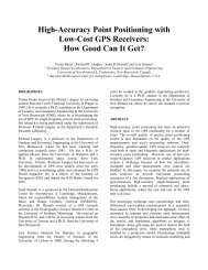
Figure 2. Carrier power to noise density ratio (C/N 0 ).<br />
The red dots represent <strong>the</strong> C/N 0 values for L1 signal<br />
for PRN138 and <strong>the</strong> blue dots show <strong>the</strong> <strong>L5</strong> C/N 0 values<br />
for PRN 138. The magenta and green dots represent<br />
<strong>the</strong> L1 and <strong>L5</strong> C/N 0 values, respectively for PRN135.<br />
In Figure 2, we can first see that <strong>the</strong> overall C/N 0 values<br />
for <strong>the</strong> L1 and <strong>L5</strong> signals from both GEOs, PRN135 and<br />
PRN138, are varying in time in <strong>the</strong> range <strong>of</strong> about ±1 dB-<br />
Hz. Those variations might be explained by neutral<br />
atmospheric effects or actual transmitted power<br />
fluctuations. By comparing <strong>the</strong> C/N 0 values between<br />
PRN138 and PRN135, we can also see that <strong>the</strong> C/N 0<br />
values have clear elevation angle dependence. Also <strong>the</strong><br />
C/N 0 values from <strong>the</strong> higher elevation angle GEO,<br />
PRN138, have smaller variations in time than those <strong>of</strong><br />
PRN135.<br />
The illustrated results in Figure 2 show that <strong>the</strong> observed<br />
<strong>WAAS</strong> <strong>L5</strong> C/N 0 values are comparable with <strong>the</strong> L1 C/N 0<br />
values for both GEOs. The compiled statistics <strong>of</strong> <strong>the</strong><br />
observed C/N 0 values in <strong>the</strong> following Table 3 also shows<br />
that <strong>the</strong> C/N 0 values <strong>of</strong> <strong>the</strong> L1 and <strong>L5</strong> signals are<br />
comparable.<br />
Table 3: Statistics <strong>of</strong> <strong>the</strong> observed C/N 0 values for <strong>the</strong><br />
<strong>WAAS</strong> GEOs, PRN135 and PRN138 for a four-day<br />
continuous period. (Units: dB-Hz)<br />
SV signal Min max mean std. dev<br />
PRN138 L1 46.60 48.00 47.35 0.19<br />
<strong>L5</strong> 46.30 47.60 46.86 0.21<br />
PRN135 L1 40.80 44.30 42.85 0.48<br />
<strong>L5</strong> 41.50 44.30 42.93 0.41
Code multipath and noise level (MP) analysis<br />
In this sub-section, <strong>the</strong> multipath and noise level (MP) <strong>of</strong><br />
C1 and C5 codes for both <strong>WAAS</strong> GEOs are analyzed.<br />
The MP observables referred to frequencies L1 and <strong>L5</strong><br />
were computed using <strong>the</strong> approach described above,<br />
equations (1) to (13).<br />
In order to see a detailed view <strong>of</strong> each step <strong>of</strong> <strong>the</strong><br />
computations, <strong>the</strong> step by step results are illustrated in<br />
Figure 3 and in Figure 4.<br />
Figure 3. MP1 and related quantities for PRN138 on<br />
25 August 2008. The y-axis range <strong>of</strong> all sub-plots is<br />
fixed to 20 m.<br />
are illustrated and <strong>the</strong> compared results show that <strong>the</strong><br />
noise level <strong>of</strong> <strong>the</strong> C1-L1 observable is higher than that <strong>of</strong><br />
C5-<strong>L5</strong> observable.<br />
By comparing <strong>the</strong> second and third panels in Figure 4, we<br />
can see that <strong>the</strong> two-times ionospheric delay terms which<br />
are properly scaled to each observable C1 and C5 could<br />
be <strong>the</strong> main source <strong>of</strong> <strong>the</strong> low frequency time variations in<br />
<strong>the</strong> C5-<strong>L5</strong> observable. After removing <strong>the</strong> ionospheric<br />
term, <strong>the</strong> remaining terms are only <strong>the</strong> constant ambiguity<br />
and slowly varying hardware delays, see eqn. (8) through<br />
(13). Therefore, <strong>the</strong> MP5 observable is more or less like a<br />
constant even though <strong>the</strong>re exists a certain amount <strong>of</strong> bias<br />
which is caused by <strong>the</strong> carrier-phase ambiguities.<br />
However, <strong>the</strong> MP1 observable in <strong>the</strong> third panel in Figure<br />
3 shows different characteristics compared with <strong>the</strong> MP5<br />
observable. The characteristics <strong>of</strong> <strong>the</strong> MP1 observable<br />
could be described as a constant bias which is caused by<br />
<strong>the</strong> ambiguity and MP effect and a specific pattern <strong>of</strong><br />
unknown origin at <strong>the</strong> moment which is varying in time.<br />
If <strong>the</strong> carrier-phase ambiguities and <strong>the</strong> satellite and<br />
receiver DCB can be assumed as constant terms (see <strong>the</strong><br />
third panels <strong>of</strong> <strong>the</strong> following Figure 8), <strong>the</strong> MP1<br />
observable should behave like <strong>the</strong> MP5 observable. To<br />
see if <strong>the</strong>re exists any correlation between <strong>the</strong> computed<br />
MP values and <strong>the</strong> GEO satellite clock <strong>of</strong>fset which is<br />
provided by <strong>the</strong> <strong>WAAS</strong> GEO navigation message,<br />
correlation coefficients between <strong>the</strong> MP observables and<br />
<strong>the</strong> GEO satellite clock <strong>of</strong>fsets were computed. The<br />
results show that <strong>the</strong> correlation coefficient between MP1<br />
and GEO clock <strong>of</strong>fset was -0.360 and it was -0.110 for <strong>the</strong><br />
MP5. Those results show that <strong>the</strong>re is a minor degree <strong>of</strong><br />
correlation.<br />
To see if <strong>the</strong> time-varying term in <strong>the</strong> MP1 observable is<br />
only observed on a specific day and if it also happened for<br />
<strong>the</strong> o<strong>the</strong>r GEO, PRN135, <strong>the</strong> MP1 and MP5 observables<br />
from both GEOs were computed for a continuous four<br />
day sample and are illustrated in Figure 5. In order to<br />
better illustrate <strong>the</strong> results, <strong>the</strong> mean <strong>of</strong> computed values<br />
was removed.<br />
Figure 4. MP5 and related quantities for PRN138 on<br />
25 August 2008. The y-axis range <strong>of</strong> all sub-plots is<br />
fixed to 20 m.<br />
Figure 3 and Figure 4 show single day results <strong>of</strong> <strong>the</strong><br />
computed MP1 and MP5 values for PRN138 on 25<br />
August 2008. In <strong>the</strong> top panels, <strong>the</strong> C1-L1 observable and<br />
C5-<strong>L5</strong> observable which contain two times <strong>the</strong><br />
ionospheric delays, ambiguity, satellite and receiver<br />
differential code bias and combined carrier-phase and<br />
pseudorange MP values as described in <strong>the</strong> above eqn. (3)
Figure 5. MP1 and MP5 observables from both<br />
PRN135 and PRN138 for a continuous four day<br />
sample, from 24 August 2008 to 27 August 2008. The<br />
blue dots indicate <strong>the</strong> MP1 observables and <strong>the</strong> red<br />
dots show <strong>the</strong> MP5 observables.<br />
Figure 5 shows that <strong>the</strong> MP1 observables from both<br />
GEOs, contain a time-varying term which is not seen in<br />
<strong>the</strong> MP5 observables from both GEOs for <strong>the</strong> continuous<br />
four sample days.<br />
Figure 6. Difference between original and moving<br />
average filtered MP values for MP1 (red dots) as well<br />
as MP5 (green dots) for PRN135 and PRN138 from 24<br />
August 2008 to 27 August 2008.<br />
To see <strong>the</strong> overall performance <strong>of</strong> <strong>the</strong> <strong>L5</strong> C5 code versus<br />
<strong>the</strong> L1 C1 code in terms <strong>of</strong> <strong>the</strong> noise level, <strong>the</strong> daily r.m.s.<br />
<strong>of</strong> <strong>the</strong> high-pass filtered MP1 and MP5 for <strong>the</strong> selected<br />
continuous four days were computed and are illustrated in<br />
Figure 7.<br />
However, <strong>the</strong> time-varying term in <strong>the</strong> MP1 observables<br />
have been identified as a contribution <strong>of</strong> <strong>the</strong> satellite DCB<br />
between C1 and C5 as discussed in <strong>the</strong> following section.<br />
Since one <strong>of</strong> our purposes in this section is to see <strong>the</strong><br />
overall performance <strong>of</strong> <strong>the</strong> new <strong>L5</strong> C5 code compared to<br />
<strong>the</strong> L1 C1 code in terms <strong>of</strong> <strong>the</strong> noise level, a moving<br />
average filter was adopted to compute <strong>the</strong> final MP values<br />
in which <strong>the</strong> low frequency variations reduced. For <strong>the</strong><br />
computation, cycle-slips in <strong>the</strong> carrier-phase<br />
measurements were identified first and <strong>the</strong> moving<br />
average filter applied to each separate arc with a window<br />
size <strong>of</strong> 10 measurements for both L1 C1 and <strong>L5</strong> C5 codes.<br />
The following Figure 6 shows <strong>the</strong> time series <strong>of</strong> <strong>the</strong><br />
difference between <strong>the</strong> original and moving average<br />
filtered MP values for L1 C1 and <strong>L5</strong> C5 codes for both<br />
GEOs.<br />
In Figure 6, we can clearly see that <strong>the</strong> MP5 values have a<br />
better quality in terms <strong>of</strong> noise level compared with MP1<br />
values. This is explained by <strong>the</strong> enhanced signal structure<br />
<strong>of</strong> <strong>the</strong> new <strong>L5</strong> signals. The <strong>L5</strong> C5 code has a higher<br />
chipping rate <strong>of</strong> 10.23 Mcps than <strong>the</strong> L1 C1 code <strong>of</strong> 1.023<br />
Mcps, making <strong>the</strong> main peak in <strong>the</strong> cross-correlation<br />
function sharper by a factor <strong>of</strong> ten, and improving noise<br />
performance and mitigating <strong>the</strong> multipath effects [Enge,<br />
2003].<br />
Figure 7, r.m.s. <strong>of</strong> <strong>the</strong> MP1 and MP5 for PRN135 and<br />
for PRN138 on four continuous days from 24 August<br />
2008 to 27 August 2008.<br />
In Figure 7, <strong>the</strong> r.m.s. <strong>of</strong> MP5 for both <strong>WAAS</strong> GEOs,<br />
show a better quality than that <strong>of</strong> MP1 as we expected.<br />
Since PRN135 was monitored at a lower elevation angle<br />
<strong>of</strong> 7.6° compared to that <strong>of</strong> 23.9° for PRN 138, <strong>the</strong> MP1<br />
for <strong>the</strong> PRN135 was observed to be higher than that <strong>of</strong><br />
PRN138.<br />
However, interestingly, we observed that <strong>the</strong> r.m.s. <strong>of</strong> <strong>the</strong><br />
MP5 values <strong>of</strong> PRN135 and PRN138 were comparable<br />
and <strong>the</strong> ranges <strong>of</strong> day-to-day variations were small. This<br />
might indicate <strong>the</strong> actual improvement <strong>of</strong> <strong>the</strong> enhanced<br />
signal structure for <strong>the</strong> <strong>WAAS</strong> <strong>L5</strong> signals compared to <strong>the</strong><br />
<strong>WAAS</strong> L1 C1 code.
Satellite & receiver differential code bias (DCB)<br />
Since <strong>WAAS</strong> GEOs broadcast <strong>the</strong> dual-frequency, L1 and<br />
<strong>L5</strong> data on <strong>the</strong> air, <strong>the</strong> ionospheric delays as well as<br />
satellite and receiver DCB should be estimated and<br />
compensated for when generating two independent<br />
signals, L1 and <strong>L5</strong>, which are uplinked to <strong>the</strong> GEOs.<br />
To identify <strong>the</strong> overall behavior <strong>of</strong> DCBs in <strong>the</strong> GPS<br />
satellites and <strong>WAAS</strong> GEOs, we first generated <strong>the</strong> DCB<br />
observables for GPS PRN10 by use <strong>of</strong> <strong>the</strong> eqn. (14)<br />
through eqn. (20) on 25 August 2008. However, since<br />
GPS does not currently provide an <strong>L5</strong> signal, <strong>the</strong> dualfrequency<br />
data, L1 C1 measurement and L2 P2<br />
measurement were used to generate DCB observables.<br />
However, note in this section that we also used <strong>the</strong> same<br />
term, DCB to represent <strong>the</strong> differential carrier-phase bias<br />
for a simplification.<br />
In <strong>the</strong> second panel, <strong>the</strong> observed slant ionospheric delays<br />
using pseudoranges are much noisier than those <strong>of</strong> carrierphase<br />
measurements and also show that <strong>the</strong> noise level <strong>of</strong><br />
<strong>the</strong> ionospheric measurements is elevation angle<br />
dependent as we expected. However, <strong>the</strong> overall<br />
variations <strong>of</strong> <strong>the</strong> observed pseudorange ionospheric delays<br />
in time are <strong>the</strong> same as those <strong>of</strong> <strong>the</strong> carrier-phase<br />
ionospheric measurements except for a residual bias<br />
which is caused by not fully accounting for <strong>the</strong> ambiguity<br />
in <strong>the</strong> carrier-phase measurements.<br />
Since we used <strong>the</strong> <strong>WAAS</strong> ionospheric corrections as a<br />
reference to generate <strong>the</strong> DCB observables (see <strong>the</strong><br />
equation (20)), <strong>the</strong> different DCBs for carrier-phase and<br />
pseudorange ionospheric measurements in <strong>the</strong> third panel<br />
could be generated. And <strong>the</strong> differences between carrierphase<br />
DCB and pseudorange DCB in <strong>the</strong> third panel<br />
could be explained by <strong>the</strong> residual carrier-phase<br />
ambiguity as well as difference in <strong>the</strong> hardware delay bias<br />
between carrier-phase and pseudoranges observables.<br />
However, with this approach, it should be noted that <strong>the</strong><br />
accuracy <strong>of</strong> <strong>the</strong> computed DCBs are dependent on <strong>the</strong><br />
accuracy <strong>of</strong> <strong>the</strong> <strong>WAAS</strong> ionospheric corrections. The user<br />
ionospheric range errors (UIRE) [<strong>WAAS</strong> MOPS., 2001]<br />
for <strong>the</strong> <strong>WAAS</strong> ionospheric delay corrections varied from<br />
0.3 m to 2.9 m for this satellite. With that accuracy, it<br />
might not be enough to precisely determine <strong>the</strong> different<br />
hardware delay biases between pseudranges and carrierphases<br />
observables.<br />
However, both computed DCBs using pseudorange and<br />
carrier-phase do not vary significantly in time indicating<br />
that <strong>the</strong> combined satellite and receiver bias is almost<br />
constant.<br />
Figure 8. Computed satellite and receiver combined<br />
DCB for GPS PRN10 on 25 August 2008. The red dots<br />
in <strong>the</strong> second panel show <strong>the</strong> computed relative<br />
ionospheric delays by using L1 and L2 carrier phase<br />
measurements and <strong>the</strong> blue dots represent <strong>the</strong><br />
ionospheric delays computed by using <strong>WAAS</strong><br />
ionospheric corrections and <strong>the</strong> green dots show <strong>the</strong><br />
computed ionospheric delays using C1 and P2<br />
pseudorange measurements. The red dots in <strong>the</strong> third<br />
panel show computed carrier phase DCB and <strong>the</strong> blue<br />
dots show <strong>the</strong> computed pseudorange DCB.<br />
Figure 8 shows <strong>the</strong> computed combined satellite and<br />
receiver DCB for <strong>the</strong> pseudorange measurements and <strong>the</strong><br />
carrier-phase measurements for GPS PRN10 on 25<br />
August 2008. Since PRN10 has few cycle slips on this<br />
day, and it <strong>the</strong>refore has a long arc with <strong>the</strong> elevation<br />
angle from 10° to about 85°, this satellite has been chosen<br />
to illustrate <strong>the</strong> DCB on GPS observations.<br />
To take advantage <strong>of</strong> <strong>the</strong> precise but ambiguous carrierphase<br />
ionospheric observables versus <strong>the</strong> unambiguous<br />
but less precise pseudorange ionospheric observables, <strong>the</strong><br />
carrier-phase leveling technique was used [Komjathy,<br />
1997]:<br />
I<br />
combi<br />
∑<br />
j<br />
( ϕ j<br />
j=<br />
1<br />
= I −<br />
i<br />
n<br />
n<br />
P<br />
I<br />
∑<br />
j=<br />
1<br />
− I<br />
j<br />
Pj<br />
)<br />
ϕ<br />
(21)<br />
P<br />
where i and j are indices for <strong>the</strong> ionospheric observables<br />
starting at <strong>the</strong> beginning <strong>of</strong> an arc, i=1,2, …, n with <strong>the</strong><br />
total number <strong>of</strong> ionospheric measurements, n, used to<br />
compute <strong>the</strong> <strong>of</strong>fset between <strong>the</strong> carrier-phase ionospheric<br />
observables and pseudorange ionospheric observables and<br />
I<br />
comb i<br />
is <strong>the</strong> combined ionospheric measurement between<br />
<strong>the</strong> carrier-phase ionospheric measurement, I ϕ<br />
, and<br />
i<br />
pseudorange ionospheric measurement, I<br />
P i<br />
. In general,<br />
<strong>the</strong> weight, P<br />
j<br />
is determined based on an elevation angle
<strong>of</strong> <strong>the</strong> measurement at <strong>the</strong> specific epoch j. To compute<br />
<strong>the</strong> amount <strong>of</strong> leveling, twenty epochs (10 minutes) <strong>of</strong><br />
data used.<br />
And <strong>the</strong> final DCB values were computed based on those<br />
leveled ionospheric observables versus <strong>the</strong> <strong>WAAS</strong><br />
ionospheric corrections (see <strong>the</strong> third panel in Figure 9).<br />
Figure 10. Correlation between estimated DCB and<br />
<strong>the</strong> <strong>WAAS</strong> MP1 for PRN138.<br />
Figure 9. Computed satellite and receiver combined<br />
differential code bias (DCB) for <strong>WAAS</strong> PRN 138 on 25<br />
August 2008. In <strong>the</strong> second panel, <strong>the</strong> red dots show<br />
<strong>the</strong> computed ionospheric delays using <strong>WAAS</strong><br />
ionospheric corrections and <strong>the</strong> blue dots represent<br />
<strong>the</strong> carrier-phase leveled ionospheric delays.<br />
In Figure 9, <strong>the</strong> top panel shows <strong>the</strong> elevation angle<br />
change over a day for PRN138. It shows that even though<br />
PRN138 is a geostationary satellite, <strong>the</strong>re is some degree<br />
<strong>of</strong> movement. In <strong>the</strong> second panel, <strong>the</strong> leveled ionospheric<br />
delays could be identified as having more variations in<br />
time than <strong>the</strong> ionospheric delays computed from <strong>the</strong><br />
<strong>WAAS</strong> corrections. And finally, <strong>the</strong> differences between<br />
leveled ionospheric delays and <strong>WAAS</strong> ionospheric delays<br />
were computed as DCB estimates and illustrated in <strong>the</strong><br />
third panel.<br />
To see if <strong>the</strong>re is any correlation between estimated DCB<br />
values and <strong>the</strong> time variations which we observed in <strong>the</strong><br />
<strong>WAAS</strong> MP1 observable, a correlation analysis has been<br />
conducted.<br />
Since <strong>the</strong> receiver DCB is common for all <strong>the</strong> monitored<br />
satellites at UNB and observed as more or less constant in<br />
time as we saw in Figure 8, we took a mean <strong>of</strong> computed<br />
DCBs for all satellites and subtracted that value from <strong>the</strong><br />
computed DCBs. In this case, <strong>the</strong> remaining term<br />
represents <strong>the</strong> variation <strong>of</strong> <strong>the</strong> satellite DCB versus <strong>the</strong><br />
constant mean and which is illustrated in <strong>the</strong> first panel <strong>of</strong><br />
<strong>the</strong> Figure 10. To compare <strong>the</strong> overall correlation between<br />
estimated DCB and MP1 at <strong>the</strong> same level, <strong>the</strong> mean bias<br />
<strong>of</strong> all <strong>the</strong> MP1 values is also removed and illustrated in<br />
<strong>the</strong> second panel <strong>of</strong> Figure 10.<br />
Finally, we can see that <strong>the</strong>re is a strong anti-correlation<br />
between <strong>the</strong> variations <strong>of</strong> satellite DCB and <strong>the</strong> MP1<br />
value. The correlation coefficient between <strong>the</strong> satellite<br />
DCB and <strong>the</strong> MP1 values was -0.856. <strong>WAAS</strong> currently<br />
does not provide <strong>the</strong> C1-C5 DCB value in <strong>the</strong> transmitted<br />
<strong>WAAS</strong> messages. However, if <strong>the</strong> <strong>WAAS</strong> satellites<br />
operated in <strong>the</strong> same way as GPS satellites, single<br />
frequency <strong>WAAS</strong> GEO ranging users would need <strong>the</strong><br />
DCB value to resolve <strong>the</strong> clock referencing issue to use<br />
single frequency code observation for positioning. To<br />
circumvent this issue, it appears <strong>WAAS</strong> compensates for<br />
<strong>the</strong> C1-C5 bias in producing <strong>the</strong> L1 signal at <strong>the</strong> control<br />
segment. In this way, <strong>the</strong> single-frequency <strong>WAAS</strong> GEO<br />
ranging user does not need to consider <strong>the</strong> satellite DCB<br />
term.<br />
Positioning domain results<br />
To see if <strong>the</strong> C1-C5 satellite DCB have been compensated<br />
for producing <strong>WAAS</strong> GEO L1 C1 signals, <strong>the</strong> residuals<br />
from processing <strong>the</strong> C1 code for PRN138 in positiondetermination<br />
s<strong>of</strong>tware have been analyzed. To process<br />
GPS plus PRN138 L1 C1 pseudoranges, <strong>the</strong> UNB<br />
WADGPS point positioning s<strong>of</strong>tware [Rho and Langley,<br />
2003 and 2005] has been used.<br />
The overall processing scheme for <strong>the</strong> GPS plus PRN138<br />
L1 C1 pseudorange is:<br />
• <strong>WAAS</strong> satellite orbit and clock corrections were<br />
applied for GPS satellites: <strong>WAAS</strong> does not provide<br />
<strong>the</strong> GEOs orbit and clock corrections, above and<br />
beyond <strong>the</strong> GEO orbit and clock data in <strong>WAAS</strong><br />
messages.<br />
• <strong>WAAS</strong> ionosphere delay corrections have been<br />
applied for both GPS satellites and PRN138.
• UNB3 tropospheric delay model including Niell<br />
mapping functions used to mitigate <strong>the</strong> troposphere<br />
errors for both GPS satellites and PRN138.<br />
• To account for receiver noise and multipath, an<br />
elevation angle dependent empirical stochastic model<br />
was used.<br />
However, since <strong>the</strong> residual GPS orbit and clock errors<br />
(less than 1 m) and <strong>the</strong> <strong>WAAS</strong> GEO orbit and clock<br />
errors (more than 10 m based on GEO user range error<br />
(URA)) are different, different weighting schemes have<br />
been applied. For <strong>the</strong> GPS satellites, <strong>the</strong> initial GPS orbit<br />
error was set to 3 m (see UNB Website, [2008], <strong>the</strong> GPS<br />
orbit errors in <strong>the</strong>se days are less than 2 m) but after<br />
<strong>WAAS</strong> orbit corrections for GPS satellites, residual errors<br />
are less than 1 m and it was 10 m for <strong>the</strong> PRN138. The<br />
GEO satellite accuracy <strong>of</strong> 10 m was determined based on<br />
<strong>the</strong> given GEO user range accuracy (URA) provided by<br />
<strong>the</strong> <strong>WAAS</strong> GEO navigation message and analyzing <strong>the</strong><br />
positioning results. In most case, <strong>the</strong> URA index <strong>of</strong> <strong>the</strong><br />
<strong>WAAS</strong> GEO satellites was 6 which indicated that <strong>the</strong><br />
accuracy <strong>of</strong> GEO orbit is in <strong>the</strong> range <strong>of</strong> 13.65 m to 24.0<br />
m [IS-GPS-200D]. However, <strong>the</strong> 10 m which was used<br />
for <strong>the</strong> positioning process was determined as a slightly<br />
optimistic minimum for <strong>the</strong> initial error which can make a<br />
best result in this setup <strong>of</strong> <strong>the</strong> point positing process.<br />
were used toge<strong>the</strong>r, <strong>the</strong> 95 th percentile horizontal error<br />
was <strong>the</strong> same and 1.087 m for <strong>the</strong> 95 th percentile vertical<br />
error.<br />
Those small effects in <strong>the</strong> positioning results by<br />
additionally using <strong>WAAS</strong> GEO ranging to <strong>the</strong> GPS<br />
measurements might be explained by <strong>the</strong> weight scheme<br />
that we used. Because <strong>of</strong> <strong>the</strong> low elevation angle <strong>of</strong> <strong>the</strong><br />
PRN138 measurements with relatively less accurate GEO<br />
orbits than GPS, <strong>the</strong> weight <strong>of</strong> <strong>the</strong> GEO measurements<br />
was set to be much less than that <strong>of</strong> <strong>the</strong> GPS<br />
measurements. Therefore, <strong>the</strong> contributions <strong>of</strong> <strong>the</strong> <strong>WAAS</strong><br />
GEO ranging measurements were not significant<br />
compared with <strong>the</strong> GPS measurements in this point<br />
positioning process for <strong>the</strong> particular data set used with a<br />
large number <strong>of</strong> GPS satellites observed.<br />
However, as <strong>the</strong> first panel in Figure 11 shows, <strong>the</strong> benefit<br />
<strong>of</strong> using <strong>the</strong> <strong>WAAS</strong> GEO ranging measurements in <strong>the</strong><br />
point positing process is in <strong>the</strong> improvement <strong>of</strong> dilution <strong>of</strong><br />
precision (DOP) values. So it might be more beneficial to<br />
use <strong>WAAS</strong> GEO ranging measurements in more<br />
challenging situations where <strong>the</strong> number <strong>of</strong> monitored<br />
GPS satellites is quickly changing and/or fewer satellites<br />
are monitored as in a kinematic situation. Likely in such<br />
situations, <strong>the</strong>re will also be better positioning results if<br />
both <strong>WAAS</strong> GEOs are used for positioning as well as<br />
GPS satellites.<br />
To see <strong>the</strong> residual errors for <strong>WAAS</strong> PRN138 compared<br />
with those <strong>of</strong> GPS satellites, <strong>the</strong>y are illustrated in Figure<br />
12.<br />
Figure 11. Benefit <strong>of</strong> using <strong>WAAS</strong> GEO ranging in<br />
point positioning. The top panel shows <strong>the</strong> number <strong>of</strong><br />
satellites which have been used for <strong>the</strong> point<br />
positioning process and PDOP. The green trace shows<br />
<strong>the</strong> results <strong>of</strong> using GEO ranging data and <strong>the</strong> red<br />
trace shows <strong>the</strong> results without using <strong>WAAS</strong> GEO<br />
ranging measurements.<br />
In Figure 11, <strong>the</strong> overall improvement <strong>of</strong> using <strong>the</strong><br />
<strong>WAAS</strong> GEO satellite is negligible in <strong>the</strong> positioning<br />
results. The 95 th percentile horizontal error was 0.783 m<br />
and <strong>the</strong> 95 th percentile vertical error was 1.091 m when<br />
only <strong>the</strong> GPS measurements were used. When <strong>the</strong> GPS as<br />
well as <strong>the</strong> <strong>WAAS</strong> GEO PRN138 ranging measurements<br />
Figure 12. Residual errors for L1 C1 for PRN138 and<br />
GPS satellites (top panel) and PRN138 alone (bottom<br />
panel) on 25 August 2008.<br />
The top panel in <strong>the</strong> Figure 12 shows all <strong>the</strong> residual<br />
errors for <strong>the</strong> GPS satellites as well as <strong>WAAS</strong> PRN138<br />
versus elevation angle. The residual errors <strong>of</strong> PRN138 are<br />
displayed at about 24° elevation angle and show more<br />
than 4 times bigger residual errors than <strong>the</strong> residuals <strong>of</strong>
GPS satellites at <strong>the</strong> same elevation angle. Since <strong>the</strong><br />
ionosphere and troposphere errors have been corrected,<br />
<strong>the</strong> dominant error sources are likely <strong>the</strong> residual GEO<br />
orbit and clock errors. The overall range <strong>of</strong> <strong>the</strong> residual<br />
error variations were observed at about ±4 m level. This<br />
figure indicates that a proper weighting scheme needs to<br />
be used for <strong>WAAS</strong> GEO range measurements in <strong>the</strong><br />
positioning domain.<br />
Finally, <strong>the</strong> second panel in Figure 12 shows <strong>the</strong> time<br />
series <strong>of</strong> <strong>the</strong> residual errors for PRN138. By comparing<br />
Figure 10 and Figure 12, we observed <strong>the</strong>re are no strong<br />
correlations between <strong>the</strong> overall variation <strong>of</strong> <strong>the</strong> PRN138<br />
residual errors and <strong>the</strong> estimated satellite DCB. The<br />
correlation coefficient between C1 residuals and <strong>the</strong><br />
estimated satellite DCB was -0.165.<br />
CONCLUSIONS<br />
The quality <strong>of</strong> <strong>the</strong> new <strong>WAAS</strong> <strong>L5</strong> signal has been<br />
evaluated by comparing selected signal quality indices for<br />
<strong>the</strong> L1 and <strong>L5</strong> signals.<br />
C/N 0 values for <strong>the</strong> <strong>WAAS</strong> GEOs, PRN135 and PRN138,<br />
have been compared on <strong>the</strong> L1 and <strong>L5</strong> frequencies. The<br />
result showed that <strong>the</strong> signal strength <strong>of</strong> <strong>WAAS</strong> <strong>L5</strong> is not<br />
stronger than L1 but ra<strong>the</strong>r reaches similar values, within<br />
±1 dB-Hz, as those <strong>of</strong> <strong>the</strong> C/N 0 <strong>of</strong> <strong>the</strong> C1 code on <strong>the</strong> L1<br />
frequency.<br />
By comparing <strong>the</strong> multipath plus noise level between L1<br />
C1 and <strong>L5</strong> C5 codes, we found that <strong>the</strong> enhanced signal<br />
structure <strong>of</strong> <strong>the</strong> <strong>L5</strong> has a better quality in terms <strong>of</strong><br />
multipath plus noise level compared to <strong>the</strong> L1 C1 code.<br />
Currently, <strong>the</strong> <strong>WAAS</strong> control segment is using dual<br />
frequency data from <strong>the</strong> GEOs. By examining <strong>the</strong><br />
multipath plus noise and estimated DCB values, we found<br />
that <strong>WAAS</strong> GEO satellite DCBs appear to be varying in<br />
time and that <strong>the</strong> <strong>WAAS</strong> control segment compensates for<br />
<strong>the</strong> C1-C5 DCB bias when producing <strong>the</strong> L1 C1 signal.<br />
The residual errors in <strong>the</strong> positioning domain results<br />
indicate that a proper weighting scheme should be used<br />
for incorporating <strong>WAAS</strong> GEO range measurements as<br />
additional to <strong>the</strong> GPS measurements in <strong>the</strong> positioning<br />
domain.<br />
It should be pointed out that although <strong>WAAS</strong> currently<br />
transmits <strong>L5</strong> signals, <strong>the</strong>y are not intended for end users at<br />
this time.<br />
ACKNOWLEDGMENTS<br />
The research reported in this paper was supported by <strong>the</strong><br />
Natural Sciences and Engineering Research Council <strong>of</strong><br />
Canada and <strong>the</strong> GEOID Network <strong>of</strong> Centres <strong>of</strong><br />
Excellence. The authors would like to thank NovAtel Inc.<br />
for allowing us to use <strong>the</strong>ir special firmware as well as for<br />
<strong>the</strong> receiver used in this research.<br />
REFERENCES<br />
Enge, Per (2003). “GPS Modernization: Capabilities <strong>of</strong><br />
<strong>the</strong> <strong>New</strong> Civil <strong>Signal</strong>s.” Invited Paper for <strong>the</strong> Australian<br />
International Aerospace Congress Brisbane, 29 July – 1<br />
August.<br />
Grewal, Mohinder S. (2008). “GNSS Solutions: <strong>WAAS</strong><br />
Functions and Differential Biases.” InsideGNSS, Vol. 3,<br />
No. 4, May/June, pp. 18-23.<br />
Hsu, Po-Hsin, L. Cheung and M. Grewal (2004).<br />
“Prototype Test Results <strong>of</strong> L1/<strong>L5</strong> <strong>Signal</strong>s <strong>of</strong> Future GEO<br />
Satellites.” Proceedings <strong>of</strong> ION GNSS 2004, 17th<br />
International Technical Meeting <strong>of</strong> <strong>the</strong> Satellite Division<br />
<strong>of</strong> The Institute <strong>of</strong> Navigation, Long Beach, CA, 21-24<br />
September 2004, pp. 1359-1366.<br />
Hsu, Po-Hsin, L. Cheung and M. Grewal (2007). “Method<br />
and Apparatus for Wide Area Augmentation System<br />
Having L1/<strong>L5</strong> Bias Estimation.” United States Patent<br />
20070067073, International Publication Date 5 April<br />
2007.<br />
IS-GPS-200D (2004). “NAVSTAR GPS Space<br />
Segment/Navigation User Interfaces.” GPS Joint Program<br />
Office, 7 December.<br />
IS-GPS-705 (2005). “NAVSTAR GPS Space<br />
Segment/Navigation User Interfaces.” GPS Joint Program<br />
Office, Revision, IRN-705-003, 22 September 2005.<br />
Komjathy, A. (1997). “Global Ionospheric Total Electron<br />
Content Mapping Using <strong>the</strong> Global Positioning System.”<br />
Ph. D dissertation, Department <strong>of</strong> Geodesy and<br />
Geomatics Engineering Technical Report No. 188,<br />
<strong>University</strong> <strong>of</strong> <strong>New</strong> <strong>Brunswick</strong>, Fredericton, Canada, 248<br />
pp.<br />
Rho, H., R.B. Langley, and A. Kassam (2003). "The<br />
Canada-Wide Differential GPS Service: Initial<br />
Performance." Proceedings <strong>of</strong> ION GPS/GNSS 2003,<br />
16th International Technical Meeting <strong>of</strong> <strong>the</strong> Satellite<br />
Division <strong>of</strong> The Institute <strong>of</strong> Navigation, Portland, OR, 9-<br />
12 September 2003, pp. 425-436.<br />
Rho, H. and R.B. Langley (2005). "Dual-frequency GPS<br />
Precise Point Positioning with WADGPS Corrections."<br />
Proceedings <strong>of</strong> ION GNSS 2005, 18th International<br />
Technical Meeting <strong>of</strong> The Institute <strong>of</strong> Navigation, Long<br />
Beach, CA, 13-16 September 2005, pp. 1470-1482.
Schempp, T. R. (2008). “Good, Better, Best: Expanding<br />
<strong>the</strong> Wide Area Augmentation System.” GPS World, Vol.<br />
19, No 1, January, pp. 62-67.<br />
UNB Website (2008): “GPS Broadcast Orbit Accuracy<br />
Statistics”, http://gge.unb.ca/gauss/htdocs/grads/orbit/.<br />
Accessed on September 6, 2008.<br />
Van Dierendonck, A.J and C. Hegarty (2000), “<br />
The <strong>New</strong> <strong>L5</strong> Civil GPS <strong>Signal</strong>.” GPS World, Vol. 11,<br />
No.9, pp. 64-72.<br />
<strong>WAAS</strong> MOPS (2001). “Minimum Operational<br />
Performance Standards for Global Positioning<br />
System/Wide Area Augmentation System Airborne<br />
Equipment.” RTCA Inc. Documentation No. RTCA/DO-<br />
229C, 28 November.