A combined discrete–continuous model describing the lag phase of ...

174 R.C. McKellar, K. Knight / International Journal of Food Microbiology 54 (2000) 171 –180
Table 1
Kinetic parameters for Listeria monocytogenes determined using
a
the Bioscreen
Trial t m t S.D. % Growth
d L L
(n520)
A 20.35 1.04 5.86 0.783 60
B 21.32 0.876 4.12 0.814 65
a 21
t
d, Time to detection (h); m, specific growth rate (h ); t
L,
mean individual cell lag phase duration (h); S.D.
L, standard
deviation of the mean individual lag phase duration; % growth,
percent of wells showing growth.
single cell per well can be calculated from a Poisson
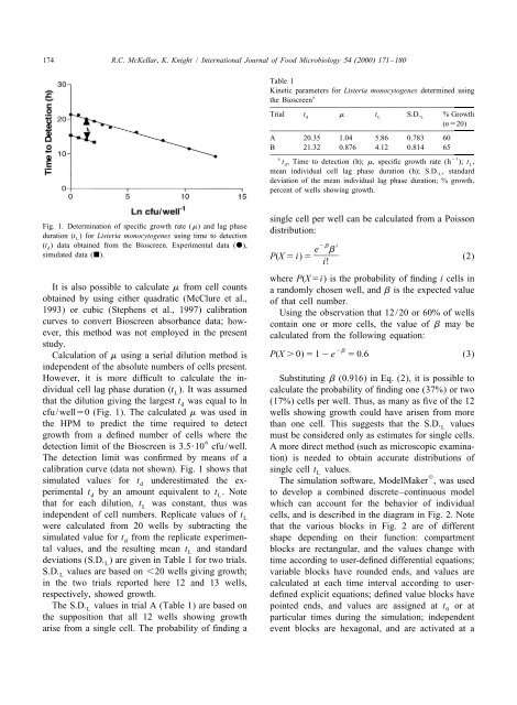
Fig. 1. Determination of specific growth rate (m) and lag phase
duration (t
L) for Listeria monocytogenes using time to detection
distribution:
(t ) data obtained from the Bioscreen. Experimental data (d),
2b i
d
e b
simulated data (j). P(X 5 i) 5 ]]
i!
(2)
where P(X5i) is the probability of finding i cells in
It is also possible to calculate m from cell counts a randomly chosen well, and b is the expected value
obtained by using either quadratic (McClure et al., of that cell number.
1993) or cubic (Stephens et al., 1997) calibration Using the observation that 12/20 or 60% of wells
curves to convert Bioscreen absorbance data; how- contain one or more cells, the value of b may be
ever, this method was not employed in the present calculated from the following equation:
study.
Calculation of m using a serial dilution method is
independent of the absolute numbers of cells present.
2b
P(X . 0) 5 1 2 e 5 0.6 (3)
However, it is more difficult to calculate the in- Substituting b (0.916) in Eq. (2), it is possible to
dividual cell lag phase duration (t
L). It was assumed calculate the probability of finding one (37%) or two
that the dilution giving the largest td
was equal to ln (17%) cells per well. Thus, as many as five of the 12
cfu/well50 (Fig. 1). The calculated m was used in wells showing growth could have arisen from more
the HPM to predict the time required to detect than one cell. This suggests that the S.D.
L
values
growth from a defined number of cells where the must be considered only as estimates for single cells.
6
detection limit of the Bioscreen is 3.510 cfu/well. A more direct method (such as microscopic examina-
The detection limit was confirmed by means of a tion) is needed to obtain accurate distributions of
calibration curve (data not shown). Fig. 1 shows that single cell tL
values.
©
simulated values for t underestimated the ex- The simulation software, ModelMaker , was used
d
perimental td
by an amount equivalent to t
L. Note to develop a combined discrete–continuous model
that for each dilution, tL
was constant, thus was which can account for the behavior of individual
independent of cell numbers. Replicate values of t cells, and is described in the diagram in Fig. 2. Note
L
were calculated from 20 wells by subtracting the that the various blocks in Fig. 2 are of different
simulated value for td
from the replicate experimen- shape depending on their function: compartment
tal values, and the resulting mean tL
and standard blocks are rectangular, and the values change with
deviations (S.D. ) are given in Table 1 for two trials. time according to user-defined differential equations;
L
S.D.
L
values are based on ,20 wells giving growth; variable blocks have rounded ends, and values are
in the two trials reported here 12 and 13 wells, calculated at each time interval according to userrespectively,
showed growth.
defined explicit equations; defined value blocks have
The S.D.
L
values in trial A (Table 1) are based on pointed ends, and values are assigned at t0
or at
the supposition that all 12 wells showing growth particular times during the simulation; independent
arise from a single cell. The probability of finding a
event blocks are hexagonal, and are activated at a