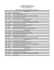
Active and Driven Soft Matter Lecture 3 - Boulder School for ...

The Model
A Tutorial: From Langevin equation to Hydrodynamics
Smoluchowski equation for SP rods
Hydrodynamics
Results
Summary and Outlook
Active and Driven Soft Matter
Lecture 3: Self-Propelled Hard Rods
M. Cristina Marchetti
Syracuse University
Boulder School 2009
Marchetti Active and Driven Soft Matter: Lecture 3

The Model
A Tutorial: From Langevin equation to Hydrodynamics
Smoluchowski equation for SP rods
Hydrodynamics
Results
Summary and Outlook
Lecture 1: Table of Contents
1 The Model
Active Hard Rod Nematic
Plan and Results
2 A Tutorial: From Langevin equation to Hydrodynamics
Langevin dynamics
From Langevin to Fokker-Planck dynamics
Low density limit & Smoluchowski equation
Hydrodynamics
Summary and Plan
3 Smoluchowski equation for SP rods
Langevin dynamics of SP Rods
Smoluchowski equation for SP rods
4 Hydrodynamics
Hydrodynamics Fields
Hydrodynamics Equations
5 Results
Homogeneous States and Enhanced Nematic Order
Stability and Novel Properties of Bulk States
6 Summary and Outlook
Marchetti Active and Driven Soft Matter: Lecture 3

The Model
A Tutorial: From Langevin equation to Hydrodynamics
Smoluchowski equation for SP rods
Hydrodynamics
Results
Summary and Outlook
Active Hard Rod Nematic
Active Hard Rod Nematic
Plan and Results
•2d hard rods
•Excluded volume interaction
•Overdamped dynamics
•Non-thermal white noise
hard rod nematic
+ self-propulsion v 0
along long axis
v 0
1. Start with Langevin dynamics of coupled orientational and
translational degrees of freedom plus hard core collisions
SP yields anisotropic enhancement of
ˆk
momentum transferred in a hard core
1
collision
v 1
v2
2. Derive continuum theory
2
Marchetti Active and Driven Soft Matter: Lecture 3

The Model
A Tutorial: From Langevin equation to Hydrodynamics
Smoluchowski equation for SP rods
Hydrodynamics
Results
Summary and Outlook
Plan and Results
Active Hard Rod Nematic
Plan and Results
The lecture illustrates how to use the tools of statistical physics to derive
hydrodynamics from microscopic dynamics for a minimal model of a
self-propelled system.
Inspired by Vicsek model of SP point particles that align with neighbors
according to prescribed rules in the presence of noise. This rule-based
model orders in polar (moving) states below a critical value of the noise.
Hard rods order in nematic states due to steric effects: can excluded
volume interactions, plus self-propulsion, yield a polar state
Result: no homogeneous polar state, but other nonequilibrium effects:
SP enhances nematic order
SP enhances longitudinal diffusion ("persistent" random walk)
SP yields propagating sound-like waves in the isotropic state
SP destabilizes the nematic state
SP+boundary effects can yield a polar state
Marchetti Active and Driven Soft Matter: Lecture 3

The Model
A Tutorial: From Langevin equation to Hydrodynamics
Smoluchowski equation for SP rods
Hydrodynamics
Results
Summary and Outlook
Langevin dynamics
Langevin dynamics
From Langevin to Fokker-Planck dynamics
Low density limit & Smoluchowski equation
Hydrodynamics
Summary and Plan
Spherical particle of radius a and mass m, in one dimension
m dv
dt
= −ζv + η(t) ζ = 6πηa friction
noise is uncorrelated in 〈η(t)〉 = 0
time and Gaussian: 〈η(t)η(t ′ )〉 = 2∆δ(t − t ′ )
Noise strength ∆
In equilibrium ∆ is determined by requiring
lim t→∞ < [v(t)] 2 >=< v 2 > eq = k BT
m
⇒ ∆ = ζk BT
m 2
Mean square displacement is diffusive
< [∆x(t)] 2 >= 2k [
BT
t − m (
1 − e −ζt/m)] → 2k BT
t = 2Dt
ζ ζ
ζ
Marchetti Active and Driven Soft Matter: Lecture 3

The Model
A Tutorial: From Langevin equation to Hydrodynamics
Smoluchowski equation for SP rods
Hydrodynamics
Results
Summary and Outlook
Fokker-Plank equation
Langevin dynamics
From Langevin to Fokker-Planck dynamics
Low density limit & Smoluchowski equation
Hydrodynamics
Summary and Plan
Many-particle systems
In this case it is convenient to work with phase-space distribution
functions:
ˆfN (x 1 , p 1 , x 2 , p 2 , ..., x N , p N , t) ≡ ˆf N (x N , p N , t)
These are useful when dealing with both Hamiltonian dynamics and
Langevin (stochastic) dynamics.
First step:
Transform the Langevin equation into a Fokker-Plank equation for the
noise-average distribution function
f 1 (x, p, t) =< ˆf 1 (x, p, t) >
Marchetti Active and Driven Soft Matter: Lecture 3

The Model
A Tutorial: From Langevin equation to Hydrodynamics
Smoluchowski equation for SP rods
Hydrodynamics
Results
Summary and Outlook
Fokker-Plank equation - 2
Langevin dynamics
From Langevin to Fokker-Planck dynamics
Low density limit & Smoluchowski equation
Hydrodynamics
Summary and Plan
Compact notation
dv
dt
dx
= p/m
dt
= −ζv − dU
dx + η(t)
⇒ dX
dt
= V + η(t)
„ « x
X =
p
„
«
p/m
V =
−ζv − U
„ «
′ 0
η =
η
Conservation law for probability distribution
∫ (
dX ˆf (X, t) = 1 ⇒ ∂tˆf +
∂
∂X · ∂X ˆf
)
∂t
= 0
( ) ( )
( )
∂ tˆf +
∂
∂X · Vˆf + ∂
∂X · ηˆf = 0 ⇒ ∂ tˆf + Lˆf +
∂
∂X · ηˆf = 0
∫ t
ˆf (X, t) = e −Lt f (X, 0) − ds e −L(t−s) ∂
0
∂X η(s)ˆf (x, s)
Marchetti Active and Driven Soft Matter: Lecture 3

The Model
A Tutorial: From Langevin equation to Hydrodynamics
Smoluchowski equation for SP rods
Hydrodynamics
Results
Summary and Outlook
Fokker-Plank equation - 3
Langevin dynamics
From Langevin to Fokker-Planck dynamics
Low density limit & Smoluchowski equation
Hydrodynamics
Summary and Plan
Use properties of Gaussian noise to carry out averages
∂ t < ˆf > +
∂
∂X · V < ˆf > + ∂
∂X · < η(t)e−Lt f (X, 0) >
− ∂ Z t
∂X · < η(t) ds e −L(t−s) ∂
0
∂X η(s)ˆf (X, s) > = 0
∂ t f = − p m ∂ xf − ∂ p [−U ′ (x) − ζp/m]f + ∆∂ 2 pf
Fokker-Plank eq. easily generalized to many interacting particles
dp α
= −ζv α − X ∂ xα V (x α − x β ) + η α(t)
dt
β
Z
∂ t f 1 (1, t) = −v 1 ∂ x1 f 1 (1) + ζ∂ p1 v 1 f 1 (1) + ∆∂p 2 1
f 1 (1) + ∂ p1 d2 ∂ x1 V (x 12 )f 2 (1, 2, t)
Marchetti Active and Driven Soft Matter: Lecture 3

The Model
A Tutorial: From Langevin equation to Hydrodynamics
Smoluchowski equation for SP rods
Hydrodynamics
Results
Summary and Outlook
Smoluchowski equation
Langevin dynamics
From Langevin to Fokker-Planck dynamics
Low density limit & Smoluchowski equation
Hydrodynamics
Summary and Plan
1
One obtains a hierarchy of Fokker-Planck equations for f 1 (1),
f 2 (1, 2), f 3 (1, 2, 3), ... To proceed we need a closure ansatz. Low
density (neglect correlations) f 2 (1, 2, t) ≃ f 1 (1, t)f 1 (2, t)
2
It is instructive to solve the FP equation by taking moments
c(x, t) = R dp f (x, p, t)
J(x, t) = R dp (p/m)f (x, p, t)
concentration of particles
density current
Eqs. for the moments obtained by integrating the FP equation.
∂ t c(x, t) = −∂ x J(x, t)
∂ t J(x 1 ) = −ζJ(x 1 ) − m∆
ζ ∂x 1 c(x 1) − R dx 2 [∂ x1 V (x 12 )]c(x 1 , t)c(x 2 , t)
For t >> ζ −1 , we eliminate J to obtain a Smoluchowski eq. for c
∂ t c(x 1 , t) = D∂ 2 x 1
c(x 1 , t) + 1 ζ ∂ x 1
∫x 2
[∂ x1 V (x 12 )]c(x 1 , t)c(x 2 , t)
Marchetti Active and Driven Soft Matter: Lecture 3

The Model
A Tutorial: From Langevin equation to Hydrodynamics
Smoluchowski equation for SP rods
Hydrodynamics
Results
Summary and Outlook
Hydrodynamics
Langevin dynamics
From Langevin to Fokker-Planck dynamics
Low density limit & Smoluchowski equation
Hydrodynamics
Summary and Plan
Due to the interaction with the substrate, momentum is not
conserved. The only conserved field is the concentration of particles
c(x, t). This is the only hydrodynamic field.
To obtain a hydrodynamic equation form the Smoluchowski equation we recall that we
are interested in large scales. Assuming the pair potential has a finite range R 0 , we
consider spatial variation of c(x, t) on length scales x >> R 0 and expand in gradients
∂ t c(x 1 , t) = D∂x 2 1
c(x 1 , t) + 1 Z
ζ ∂x 1
V (x ′ )[∂ x ′c(x 1 + x ′ , t)]c(x 1 , t)
x ′
= D∂x 2 1
c(x 1 , t) + 1 Z
ζ ∂x 1
V (x ′ )[∂ x1 c(x 1 , t) + x ′ ∂ 2
x ′ x 1
c(x 1 , t) + ...]c(x 1 , t)
The result is the expected diffusion equation, with a microscopic
expression for D ren which is renormalized by interactions
∂ t c(x, t) = ∂ x [D ren ∂ x c(x, t)] ≃ D ren ∂ 2 x c(x, t)
Marchetti Active and Driven Soft Matter: Lecture 3

The Model
A Tutorial: From Langevin equation to Hydrodynamics
Smoluchowski equation for SP rods
Hydrodynamics
Results
Summary and Outlook
Summary of Tutorial and Plan
Langevin dynamics
From Langevin to Fokker-Planck dynamics
Low density limit & Smoluchowski equation
Hydrodynamics
Summary and Plan
Microscopic Langevin dynamics of interacting particles
Approximations: noise average; low density: f 2 (1, 2) ≃ f 1 (1)f 1 (2)
⇓
Fokker Planck equation
⇓
Overdamped limit: t >> 1/ζ Smoluchowski equation
[
∂ t c(x 1 , t) = ∂ x1 D∂ x1 c(x 1 , t) − 1 ∫
]
F (x 12 )c(x 2 , t)c(x 1 , t
ζ x 2
Pair interaction F (x 12 ):
steric repulsion → SP rods
short-range active interactions → cross-linkers in motor-filaments mixtures
medium-mediated hydrodynamic interactions → swimmers
Smoluchowski → Hydrodynamic equations
Marchetti Active and Driven Soft Matter: Lecture 3

SP Rods
The Model
A Tutorial: From Langevin equation to Hydrodynamics
Smoluchowski equation for SP rods
Hydrodynamics
Results
Summary and Outlook
Langevin dynamics of SP Rods
Smoluchowski equation for SP rods
The algebra is quite a bit more involved for a number of reasons:
1
translational and rotational degrees of freedom are coupled
∂v α
∂t
= v 0 ˆν α − ζ(ˆν α) · v α − P β T (α, β) vα + ηα (t)
∂ω α
∂t
= −ζ R ω α − P β T (α, β) ωα + ηR α (t)
where ˙η αi (t)η βj (t ′ )¸ = 2k B T a ζ ij (ˆν α)δ ij δ (t − t ′ )
D
E
ηα R (t) ηβ R (t′ ) = 2k B T a (ζ R /I) δ αβ δ (t − t ′ ), I = l 2 /12
ζ ij (ˆν α) = ζ ‖ˆν αi ˆν αj + ζ ⊥ (δ ij − ˆν αi ˆν αj )
2
hard core interactions must be treated with care to handle
properly the instantaneous momentum transfer
3
coupling of self-propulsion and collisional dynamics yields
angular correlations
Marchetti Active and Driven Soft Matter: Lecture 3

The Model
A Tutorial: From Langevin equation to Hydrodynamics
Smoluchowski equation for SP rods
Hydrodynamics
Results
Summary and Outlook
Langevin dynamics of SP Rods
Smoluchowski equation for SP rods
Smoluchowski equation for SP rods
The Smoluchowski equation for c(r, ˆν, t) is given by
∂ t c + v 0 ∂ ‖ c = D R ∂ 2 θc + (D ‖ + D S )∂ 2 ‖ c + D ⊥∂ 2 ⊥c
−(Iζ R ) −1 ∂ θ (τ ex + τ SP ) − ∇ · ζ −1 · (F ex + F SP )
∂ ‖ = ˆν · ∇
D S = v0 2/ζ ‖ enhancement of
∂ ⊥ = ∇ − ˆν(ˆν · ∇)
longitudinal diffusion
Torques and forces exchanged upon collision as the sum of Onsager
excluded volume terms and contributions from self-propulsion:
τ ex = −∂ θ V ex
V
F ex = −∇V
ex (1) = k B T ac(1, t) R R
ξ ex
12 ˆν |ˆν
2
1 × ˆν 2 | c (r 1 + ξ 12 , ˆν 2 , t)
ξ 12 = ξ 1 − ξ 2
„ « Z !
′
FSP
= v
τ 0
2 b k
SP ẑ · (ξ 1 × b [ẑ · (ˆν 1 × ˆν 2 )] 2
k)
s 1 ,s 2
Z2,ˆk
×Θ(−ˆν 12 · bk)c(1, t)c(2, t)
Marchetti Active and Driven Soft Matter: Lecture 3

The Model
A Tutorial: From Langevin equation to Hydrodynamics
Smoluchowski equation for SP rods
Hydrodynamics
Results
Summary and Outlook
SP terms in Smoluchowski Eq.
Langevin dynamics of SP Rods
Smoluchowski equation for SP rods
Convective term describes mass flux along the rod’s long axis.
Longitudinal diffusion enhanced by self-propulsion:
D ‖ → D ‖ + v 2 0 /ζ ‖. Longitudinal diffusion of SP rod as persistent
random walk with bias ∼ v 0 towards steps along the rod’s long
axis.
The SP contributions to force and torque describe, within
mean-field, the additional anisotropic linear and angular
momentum transfers during the collision of two SP rods.
D E
√
∆pcoll
Mean-field Onsager: ∼ v th
∼
∆t τ √ kB T a
∼ k BT a
coll l/ k B T a
l
D E
∆pcoll
SP rods: ∆t ∼ v 0| ˆν 1 × ˆν 2 |
SP
l/v 0 | ˆν 1 × ˆν 2 | ∼ v 0 2|ˆν 1 × ˆν 2 | 2
Marchetti Active and Driven Soft Matter: Lecture 3

The Model
A Tutorial: From Langevin equation to Hydrodynamics
Smoluchowski equation for SP rods
Hydrodynamics
Results
Summary and Outlook
Hydrodynamics Fields
Hydrodynamics Fields
Hydrodynamics Equations
Conserved density: ρ(r, t) = ∫ c(r, ˆν, t)
ˆν
Order parameter fields:
Polarization vector:
P(r, t) = ∫ ˆν c(r, ˆν, t)
ˆν
Polar order
p -p
fish, bacteria,
motor-filaments
p
Nematic alignment tensor:
Q ij (r, t) = ∫ ˆν (ˆν i ˆν j − 1 2 δ ij)c(r, ˆν, t)
Nematic
order
n -n
melanocytes,
granular rods
n
Marchetti Active and Driven Soft Matter: Lecture 3

The Model
A Tutorial: From Langevin equation to Hydrodynamics
Smoluchowski equation for SP rods
Hydrodynamics
Results
Summary and Outlook
Hydrodynamics Equations
Hydrodynamics Fields
Hydrodynamics Equations
∂ t ρ + v 0 ∇ · P = D ρ∇ 2 ρ + D Q ∇∇ : ρQ
∂ t P = −D R P + λP · Q − v 0 ∇ · Q − λ 1 (P · ∇)P − λ 2 ∇P 2 − λ 3 P(∇ · P)
− v 0
2 ∇ρ + D bend ∇ 2 P + (D splay − D benb )∇(∇ · P)
∂ t Q = −4D R
„
1 − ρ
ρ IN
«
Q − v 0 [∇P] ST − λ 4 [P∇Q] ST − λ 5 [Q∇P] ST − λ 6 [∇P] ST
[T] ST
ij = 1 2 (T ij + T ji − 1 2 δ ij T kk )
+ D Q
4 (∇∇ − 1 2 1)ρ + D′ Q ∇2 Q
Marchetti Active and Driven Soft Matter: Lecture 3

The Model
A Tutorial: From Langevin equation to Hydrodynamics
Smoluchowski equation for SP rods
Hydrodynamics
Results
Summary and Outlook
Homogeneous States
Homogeneous States and Enhanced Nematic Order
Stability and Novel Properties of Bulk States
Neglecting all gradients, the equations are given by
Bulk states:
∂ t ρ = 0
∂ t P = −D R P + λP · Q
Isotropic State: ρ = ρ 0 , P = Q = 0
No bulk uniform polar state: P = 0
Nematic state P = 0, Q ≠ 0 for
ρ > ρ IN
SP enhances nematic order:
ρ IN =
ρ N
1+ v2 0
5k B T
∂ t Q = −4D R [1 − ρ/ρ IN (v 0 )] Q
with ρ N = 3/(πl 2 )
Marchetti Active and Driven Soft Matter: Lecture 3

The Model
A Tutorial: From Langevin equation to Hydrodynamics
Smoluchowski equation for SP rods
Hydrodynamics
Results
Summary and Outlook
Homogeneous States and Enhanced Nematic Order
Stability and Novel Properties of Bulk States
Enhanced Nematic order in Simulations of Actin
Motility Assay
-
+
Marchetti Active and Driven Soft Matter: Lecture 3

The Model
A Tutorial: From Langevin equation to Hydrodynamics
Smoluchowski equation for SP rods
Hydrodynamics
Results
Summary and Outlook
Homogeneous States and Enhanced Nematic Order
Stability and Novel Properties of Bulk States
Hydrodynamic Modes Stability of Bulk States
We examine the dynamics of the fluctuations of the hydrodynamic
fields about their mean values and analyze the hydrodynamic modes
of the system.
ρ = ρ
Isotropic state (neglect Q)
0 + δρ
P = 0 + δP
Linearized equations:
Fourier modes:
∂ t δρ = D ρ ∇ 2 δρ + v 0 ρ 0 ∇ · δP
∂ t δP = −D R δP + (v 0 /2ρ 0 )∇δρ
δρ(r, t) = ∑ k δρ k(t)e ik·r
δP(r, t) = ∑ k δP k(t)e ik·r
z ± = − 1 2 (D R + D ρ k 2 ) ± 1 2
√
(D R − D ρ k 2 ) 2 − 2v 2 0 k 2
δρ k (t) ∼ e −z(k)t
δP k (t) ∼ e −z(k)t
Marchetti Active and Driven Soft Matter: Lecture 3

The Model
A Tutorial: From Langevin equation to Hydrodynamics
Smoluchowski equation for SP rods
Hydrodynamics
Results
Summary and Outlook
Sound Waves in Isotropic State
Homogeneous States and Enhanced Nematic Order
Stability and Novel Properties of Bulk States
Propagating density waves in isotropic
state of overdamped SP rods
t
= D
2 + v 0
0P
tP = DRP + v0 0
fluctuations:
= 0
+ , P = P 0
0
+ P
v 0
Above a critical v 0 the
system supports sound-like
waves in a range of
wavevectors
v 0c
v 0c
D R
Ramaswamy & Mazenko, 1982: fluid on frictional substrate
--> movie of fluidized rods by Durian’s lab
Marchetti Active and Driven Soft Matter: Lecture 3

The Model
A Tutorial: From Langevin equation to Hydrodynamics
Smoluchowski equation for SP rods
Hydrodynamics
Results
Summary and Outlook
Instability of Nematic State
Homogeneous States and Enhanced Nematic Order
Stability and Novel Properties of Bulk States
The nematic state is unstable
for v 0 > v c (φ, S), as shown in
the figure for S = 1 (red line)
and S < 1 (dashed blue line).
The instability arises from a
subtle interplay of splay and
bend deformations.
cosφ = ˆn 0 · ˆk
φ = 0 pure bend
φ = π/2 pure splay
Marchetti Active and Driven Soft Matter: Lecture 3

The Model
A Tutorial: From Langevin equation to Hydrodynamics
Smoluchowski equation for SP rods
Hydrodynamics
Results
Summary and Outlook
Homogeneous States and Enhanced Nematic Order
Stability and Novel Properties of Bulk States
Enhanced polar order near boundaries
SP can enhance the size of correlated polar regions, as seen in
simulations [F. Peruani, A. Deutsch and M. Bär, Phys. Rev. E 74,
030904 (2006).].
Polarization profile across
channel (P x (±L/2) = P 0 )
P x (y) = P 0 cosh(y/δ)/ cosh(L/2δ)
√
δ = l/2 5/2 + v0 2/k BT
δ(v 0 = 0) ∼ l
Marchetti Active and Driven Soft Matter: Lecture 3

The Model
A Tutorial: From Langevin equation to Hydrodynamics
Smoluchowski equation for SP rods
Hydrodynamics
Results
Summary and Outlook
Summary and Outlook
A minimal model of interacting SP hard rods exhibits several
novel nonequilibrium phenomena at large scales
No bulk polar state
enhancement of nematic order
enhancement of longitudinal diffusion
sound waves in isotropic state
enhanced polarization correlations
We will consider in the last lecture a richer model that
incorporates the role of fluid flow.
References
1 R. Zwanzig, Nonequilibrium Statistical Mechanics (Oxford University Press,
2001), Chapters 1 and 2.
2 A. Baskaran and M. C. Marchetti, Hydrodynamics of Self-Propelled Hard
Rods, Phys. Rev. E 77, 011920 (2008).
3 A. Baskaran and M. C. Marchetti, Enhanced Diffusion and Ordering of
Self-Propelled Rods, Phys. Rev. Lett. 101, 268101 (2008).
Marchetti Active and Driven Soft Matter: Lecture 3