Improved Monte Carlo Localization of Autonomous Robots through ...

Improved Monte Carlo Localization of Autonomous Robots through
Simultaneous Estimation of Motion Model Parameters
Jörg Müller Christoph Gonsior Wolfram Burgard
Abstract—In recent years, there has been an increasing interest
in autonomous navigation for lightweight flying robots. With
regard to self-localization flying robots have several limitations
comparedtogroundvehicles.Duetotheirlimitedpayloadflying
vehicles possess only limited computational resources and are
restricted to a few and lightweight sensors. Additionally the
kinematics of flying robots is rather complex, which requires
sophisticated motion models that are typically hard to calibrate.
However, as the sensors provide only a limited amount of
information, the motion models need to be highly accurate
to reduce the potential increase of uncertainty caused by the
movements of the vehicle. In this paper, we present a novel
approach to simultaneous localization and estimation of motion
model parameters and their adaptation in the context of a
particle filter. To deal with sudden changes of parameters, our
approach utilizes random sampling augmented by additional
damping to avoid oscillations caused by the delayed detection
of the changes. As we demonstrate in experiments with a real
blimp, our method can deal with very sparse and imprecise
sensor information and outperforms a standard Monte Carlo
localization approach.
I. INTRODUCTION
Recently, the robotics community has shown an increasing
interest in small-sized and low-cost autonomous aerial vehicles
such as helicopters, quadrotors, or blimps. Especially
their low power consumption and safe navigation capabilities
make blimps ideally suited for long-term indoor operation
tasks. One of the most fundamental abilities of autonomously
operating robots is to localize themselves in a known environment.
This has been successfully addressed by Bayes
filter techniques in the past [22]. The smaller a flying robot
gets, however, the less sensor information is available due to
their strictly limited number of lightweight and imprecise
sensors. This increases the importance of the prediction
model of the Bayes filter localization which is often also
called the motion model of the robot. Most ground vehicles
are equipped with wheel encoders and can sense their motion
relative to the ground in a fairly accurate way. Motion
models of aerial robots, however, can not rely on direct
measurements of the velocity and in general need to estimate
accelerations due to thrust and air drag. Consequently, the
motion models are based on the complex kinematics of the
vehicle which can be modeled by physical approximations
and depends on numerous parameters. In practice, these
parameters are usually hand-tuned by a human operator or
derived from tedious calibration experiments using expert
knowledge or ground-truth pose estimates.
This work has partly been supported by the German Research Foundation
(DFG) within the Research Training Group 1103 and by the Gottfried
Wilhelm Leibniz Programme of the DFG. All authors are members of the
Department of Computer Science at the University of Freiburg, Germany
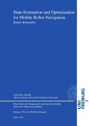
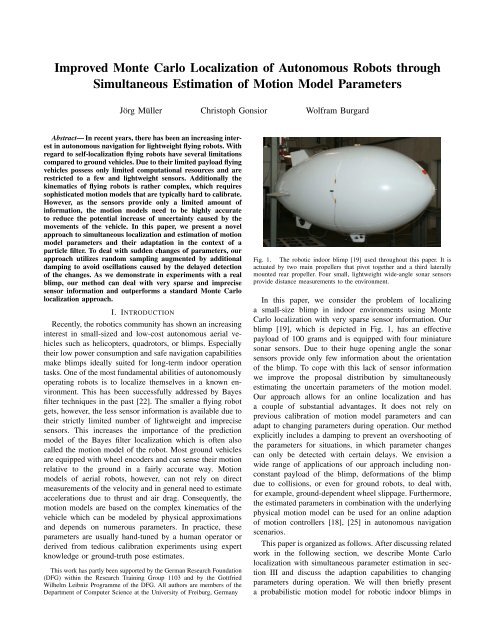
Fig. 1. The robotic indoor blimp [19] used throughout this paper. It is
actuated by two main propellers that pivot together and a third laterally
mounted rear propeller. Four small, lightweight wide-angle sonar sensors
provide distance measurements to the environment.
In this paper, we consider the problem of localizing
a small-size blimp in indoor environments using Monte
Carlo localization with very sparse sensor information. Our
blimp [19], which is depicted in Fig. 1, has an effective
payload of 100 grams and is equipped with four miniature
sonar sensors. Due to their huge opening angle the sonar
sensors provide only few information about the orientation
of the blimp. To cope with this lack of sensor information
we improve the proposal distribution by simultaneously
estimating the uncertain parameters of the motion model.
Our approach allows for an online localization and has
a couple of substantial advantages. It does not rely on
previous calibration of motion model parameters and can
adapt to changing parameters during operation. Our method
explicitly includes a damping to prevent an overshooting of
the parameters for situations, in which parameter changes
can only be detected with certain delays. We envision a
wide range of applications of our approach including nonconstant
payload of the blimp, deformations of the blimp
due to collisions, or even for ground robots, to deal with,
for example, ground-dependent wheel slippage. Furthermore,
the estimated parameters in combination with the underlying
physical motion model can be used for an online adaption
of motion controllers [18], [25] in autonomous navigation
scenarios.
This paper is organized as follows. After discussing related
work in the following section, we describe Monte Carlo
localization with simultaneous parameter estimation in section
III and discuss the adaption capabilities to changing
parameters during operation. We will then briefly present
a probabilistic motion model for robotic indoor blimps in

section IV and finally evaluate the improvements of our
localization system with simultaneous parameter estimation
in simulation and experiments with a real blimp.
II. RELATED WORK
In the past, several authors considered the problem of
localizing small flying vehicles. The majority of approaches,
however, employed previously learned motion models. For
example, Ko et al. [11] used the ground-truth estimates of
a motion capture system for tuning of the motion model.
Our previous work [15] relies on vision-based ground-truth
and uses additional IMU sensor information for localization.
Acquiring the ground-truth data involves either expensive
and bulky systems or lacks sufficient precision to infer highly
accurate motion models.
Several approaches have been proposed to improve the
proposal distribution in Monte Carlo localization using information
from sensors other than wheel encoders or control
commands. For example, Thrun et al. [23] sample additional
“dual” particles from the observation likelihood to improve
the robustness of the system and to better recover from
localization failures. Whereas this approach is very effective,
sampling from the observation likelihood is computationally
demanding for range sensors such as sonar or laser range
finders. Consequently, sampling from the observation model
was mainly used for vision-based localization. Grisetti et
al. [6] matched laser range scans to improve proposals
for wheeled robots operating on planar grounds. Later, a
similar approach was applied together with IMU data to
localize miniature quadrotors operating in 6 degrees of
freedom (DOF) [7], [9]. However, it is unclear whether small
lightweight sensors such as three miniature wide-angle sonar
sensors allow for such a scan matching approach.
One of the first systems for Monte Carlo localization with
online calibration of the motion model was developed by Roy
and Thrun [20]. They incrementally update the calibration
parameters for differential drive robots based on a maximum
likelihood position estimate obtained by scan matching.
However, their approach relies on the direct calculation of
parameters out of two consecutive pose estimates which is
not possible for more sophisticated motion models such as
those for blimps. The case of sudden changes of the models
or their parameters due to failures or collisions of wheeled
robots is addressed by Plagemann et al. [16], [17]. They
extend the particle filter localization by motion models of
different complexity and use a parameter sampling similar
to our approach. However, they assume an initially known
model including its parameters and switch online between a
finite number of models.
Beside the Monte Carlo localization, Kalman filters are a
popular technique for mobile robot localization. For example,
Martinelli et al. [14] extend the state vector by additional
parameters for odometry errors. However, motion models
of flying vehicles typically are highly non-linear and our
wide-angle sonar sensors are not suitable to use within a
Kalman filter. In the context of localization of UAVs, Bryson
and Sukkarieh [2] estimate the difference between IMU and
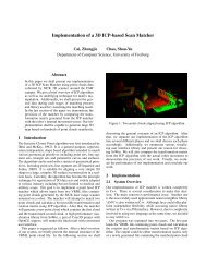
Fig. 2. The extended dynamic Bayes network for localization of a mobile
robot. It characterizes the evolution of controls u, states x, measurements
z, and parameters of the motion model Θ.
motion model prediction in an additional extended Kalman
filter to update the model parameters and the IMU bias. In
contrast to our approach this requires to update the model
parameters directly based on the prediction error similar to
Roy and Thrun [20].
Some approaches utilize the expectation maximization
algorithm to simultaneously localize a robot and adapt its
motion model. For example, Eliazar and Parr [5] iterate
between estimating the path of the robot and optimizing the
parameters of the motion model. However, these approaches
are not intended for online applications and require to quickly
optimize the parameters of the motion model given a trajectory
of the robot which is not the case, e.g., for more complex
motion models of flying robots such as blimps. Kaboli et
al. [10] use the Markov Chain Monte Carlo technique to
learn sensor and motion model parameters from raw sensor
and action data by sampling trajectories and parameters,
which typically requires substantial computational resources.
In contrast to these previous approaches, our approach
provides an online estimation and adaptation of previously
unknown parameters of a complex and potentially non-linear
motion model in the context of localization with particle
filters. Furthermore, compared to multiple model tracking
systems our approach can deal better with very slow changes
in the continuous parameter space.
III. MONTE CARLO LOCALIZATION WITH
SIMULTANEOUS PARAMETER ESTIMATION
Throughout this paper, we consider the problem of estimating
the 6-dimensional pose x = (x,y,z,φ,θ,ψ) of
a robot relative to a given map m using Monte Carlo
localization [3]. The key idea of this approach is to maintain
a probability density p(x 1:t | z 1:t ,u 1:t ) of the trajectory x 1:t
of the robot given all observations z 1:t and control inputs
u 1:t up to time t.
A. Simultaneous Parameter Estimation
In the presence of unknown (and probably time-varying)
parameters of the motion of the robot, the underlying Bayes
network is extended as depicted in Fig. 2. Here, the additional,
non-observable parameter nodes are highlighted in
gray. Consequently, the full localization posterior is extended

to p(x 1:t ,Θ 1:t | z 1:t ,u 1:t ) which can be factorized to
p(x 1:t ,Θ 1:t | z 1:t ,u 1:t ) = η · p(z t | x 1:t ,z 1:t−1 ,Θ 1:t ,u 1:t )
· p(x 1:t ,Θ 1:t | z 1:t−1 ,u 1:t ) (1)
using Bayes rule where η is a normalizer. We factorize the
second conditional probability twice and obtain
p(x 1:t ,Θ 1:t | z 1:t−1 ,u 1:t )
= p(x t ,Θ t | x 1:t−1 ,Θ 1:t−1 ,z 1:t−1 ,u 1:t )
· p(x 1:t−1 ,Θ 1:t−1 | z 1:t−1 ,u 1:t )
= p(x t | x 1:t−1 ,Θ 1:t ,z 1:t−1 ,u 1:t )
· p(Θ t | x 1:t−1 ,Θ 1:t−1 ,z 1:t−1 ,u 1:t )
· p(x 1:t−1 ,Θ 1:t−1 | z 1:t−1 ,u 1:t ) . (2)
Under the Markov assumption, (1) together with (2) can be
simplified to
p(x 1:t ,Θ 1:t | z 1:t ,u 1:t )
= η · p(z t | x t )
· p(x t | x t−1 ,Θ t ,u t )
· p(Θ t | Θ t−1 ,x 1:t−1 ,z 1:t−1 )
· p(x 1:t−1 ,Θ 1:t−1 | z 1:t−1 ,u 1:t−1 ) . (3)
As in [22], we assume that future controls give no information
about the current state of the robot.
To implement this recursive filtering scheme, we use a particle
filter [4] where a set M of weighted particles represents
the current belief. Each particle represents a hypothesis of a
robot pose and parameter vector. As the proposal distribution
we use the motion model combined with the model of the
parameter behavior
π(x 1:t ,Θ 1:t | z 1:t ,u 1:t )
= p(x t | x t−1 ,Θ t ,u t )
· p(Θ t | Θ t−1 ,x 1:t−1 ,z 1:t−1 )
· p(x 1:t−1 ,Θ 1:t−1 | z 1:t−1 ,u 1:t−1 ) , (4)
which results in the importance weight
w [i]
t = p(x 1:t,Θ 1:t | z 1:t ,u 1:t )
π(x 1:t ,Θ 1:t | z 1:t ,u 1:t )
∝ p(z t | x t ) w [i]
t−1 (5)
of the i-th particle at time t.
Assuming the parameters to be constant over time, the
belief update (3) can be performed according to the following
three alternating steps:
1) In the prediction step, we draw for each particle a new
particle according to the parameterized motion model
p(x t | x t−1 ,Θ t ,u t ) given the action u t .
2) In the correction step, we integrate a new observation
z t by assigning a new weight w [i] to each particle
according to the sensor model p(z t | x t ).
3) In the resampling step, we draw a new generation of
particles from M (with replacement) such that each
sample in M is selected with a probability that is
proportional to its weight.
Following Liu and West [12], we reduce the sample degeneracy/attrition
by adding small random disturbances to
the parameter vector of each sample during resampling.
To prevent a loss of information in the parameter vector
sampling we apply kernel smoothing
Θ [i]
t
∼ N(aΘ [i]
t−1 + (1 − a)Θ t−1,h 2 V t−1 ) , (6)
where Θ t−1 and V t−1 are the mean and the covariance of
the parameter vector over the particle set at time t − 1. The
constant factors a = 3γ−1
2γ
and h 2 = 1 − a 2 only depend on
a discount factor γ, which we set to 0.95.
B. Adaption to Changed Parameters
∑ N
i=1 p(z t | x [i]
t ) averaged over all particles.
In certain cases, we cannot assume the physical properties
of the motion of the robot to be constant for the complete
period of operation. For example, wear and tear, changed
payload, collisions, low batteries, or even manual mounting
of banner ads can change the behavior of the robot. Once
the parameter vector has converged within the particle filter,
an adaption to one or more changed parameters would
take a large number of sampling steps or could simply be
impossible.
Fortunately, this problem can be solved in a similar way as
the well-known “kidnapped robot” problem by sampling an
appropriate number of the particles at random positions [22].
We analogously cope with parameter changes by drawing the
parameter vector Θ uniformly from the parameter space for
those random samples. The proportion of random samples is
determined by monitoring the probability of sensor measurements
p = 1 N
We adopt this technique from Gutmann and Fox [8] and
extend the resampling by setting the parameter vector of each
particle to a uniform sample with probability
max
(
0,1 − p )
short
. (7)
ν p long
Here, p short and p long are short-term and long-term averages
of the sensor likelihood updated by
p short ← p short + α short (p − p short ) (8)
p long ← p long + α long (p − p long ) (9)
on each correction step with the exponential decay factors
0 < α long ≪ α short ≤ 1. The parameter ν allows to adjust
the level at which random samples are added. Thus, this
approach only adds random samples if the short-term average
of the sensor likelihood is less than ν the long-term average.
However, the sole addition of random parameter samples
does not yield superior results since the adaption to changed
parameters does not start until the pose estimate is slightly
displaced from the ground-truth caused by wrong parameters
and the average observation likelihood is dropped. When
random parameter samples are added, those particles which
quickly correct the displacement will get a higher observation
likelihood. This leads to an overshooting of the estimated
parameter values and causes the parameter values to oscillate

for several time steps (see Fig. 5, left). We address this oscillation
problem by defining a lower bound to the covariance
h 2 V, so that the parameter vectors are sampled according to
Θ [i]
t
∼ N(aΘ [i]
t−1 + (1 − a)Θ t−1,
h 2 ˜max(V t−1 ,ρ Θ t−1 Θ T t−1)) (10)
where the ˜max-operator builds a pointwise maximum over
the diagonal elements of the matrices and takes all other
elements from the first argument. Here, ρ is the relative
covariance bound. This damps the oscillation and allows for
a lower localization error after the change of parameters.
Furthermore, this approach better handles very slow changes
of parameters which are typically not detected through a
suddenly dropped observation likelihood.
Combining these techniques enables an autonomous robot
to simultaneously estimate previously unknown parameters
of the motion model in an online fashion and to adapt to
changed parameters during operation, which is especially
important in case of sparse or imprecise sensor information.
IV. PROBABILISTIC MOTION MODELS FOR MINIATURE
AIRSHIPS
The probabilistic motion model p(x t | u t ,x t−1 ) plays a
crucial role in the prediction step of the particle filter and
its proper design is essential for accurate and efficient state
estimates. An inaccurate motion model would result in a
wide-spread proposal distribution and increases the number
of wasted particles which in turn decreases the efficiency
of the filter. To define an accurate probabilistic model, we
first create a deterministic physical model of our blimp and
afterwards extend this model such that it also considers the
sources of uncertainty.
Miniature airships typically are not equipped with sensors
directly measuring their motion such as wheel encoders
found on most ground vehicles. Instead, their motion has
to be estimated based on forces and torques acting on them.
In the following, we summarize our physical motion model
which is based on [25]. The state of the blimp is defined by
its pose p = (x,y,z,φ,θ,ψ) T consisting of three Cartesian
translation coordinates and three Euler angles. Accordingly,
its velocity is v = (v x ,v y ,v z ,ω x ,ω y ,ω z ) T . The Newton-
Euler equation of motion
M dv
dt = ∑ F external (11)
couples the acceleration of the airship to the external forces
and torques. Thereby, M is the rigid-body inertia matrix and
the external forces are gravity, buoyancy, propelling forces,
air drag forces, and fictitious forces. Except for the air drag
forces, all constituent parts can be determined in a straightforward
way [25]. In the case of our blimp (see Fig. 1)
the hull cannot be approximated appropriately by a highly
symmetrical ellipsoid. Furthermore, the rear fins have an
additional stabilizing effect.
In general, two different types of air drag forces can be
distinguished: viscous resistance and quadratic drag. Since
our blimp operates at velocities exceeding 1 m s
having a
Reynolds number R e ≈ 30,000, we can safely reduce
the drag formula to the quadratic part. Consequently, we
approximate the drag force and torque of the hull in an
uncoupled way as
F D,h = ( − D x v x |v x |, −D y v y |v y |, −D z v z |v z |,
− D ′ xω x |ω x |, −D ′ yω y |ω y |, −D ′ zω z |ω z |) T . (12)
Analogously, the drag force of each fin acts parallel to its
normal and scales with its area and the fin drag coefficient
D f . Due to symmetry we can set D y = D z , D ′ y = D ′ z, and
D ′ x ≈ 0 so that the motion model depends on a vector of
four unknown parameters Θ = [D x ,D z ,D ′ z,D f ]
In our first localization system [15], we used a blimp
motion model with fixed parameters and learned those parameters
from about 8 min recorded data of our blimp based
on the reference trajectory T ∗ which was acquired using the
camera integrated in the gondola of the blimp [21]. To find
the parameter vector ˆΘ which minimizes the incremental
prediction error of the motion model we evaluated 30,000
uniformly sampled values and started a gradient descent
minimization routine from the ten best random parameter
vectors. As all of them converged to the same ˆΘ, we expect
this to be the global minimum. These previously estimated
parameters ˆΘ are not used for our proposed localization with
simultaneous parameter estimation.
The uncertainty of the motion model described above has
basically three sources of uncertainty. Firstly, the applied
physical model is only an approximation, and secondly,
the estimated parameters are not guaranteed to be the true
parameters due to imperfection of the reference trajectory
and the minimization routine. While both of these are
systematic errors, thirdly, there are statistical errors such as
imperfect motor responses, wind, or numerical errors. In our
localization system, we combine all three sources of error
and sample an additive velocity from a multivariate Gaussian
with zero mean. Its covariance was determined based on the
remaining error of the parameter optimization routine.
V. EXPERIMENTAL EVALUATION
The Monte Carlo localization with simultaneous parameter
estimation described above has been implemented and
evaluated using simulation experiments and data acquired
with a real indoor blimp. In our experiments, we consider
the problem of position tracking, i.e., localization with a
known initial pose. To address the particle depletion problem,
the resampling step is only performed if the number of
effective particles [13] n eff = (∑ i (w[i] ) 2) −1
drops below
a threshold κ. In our experiments, this is set to half the
number of particles. As a measure of localization error we
used the Euclidean distance between the weighted average
of all particles and the reference pose.
A. Experiments with a real blimp
We evaluated the improvement of the simultaneous parameter
estimation in terms of localization error using a
1.70 m long blimp [19] in a large indoor environment.
The blimp is actuated by two main propellers that pivot

translational error [m]
rotational error [degree]
success rate
1
0.8
0.6
0.4
30
25
20
15
10
1
0.8
0.6
0.4
0.2
0
extended
standard
extended
standard
extended
standard
0 2000 4000 6000 8000 10000
number of particles
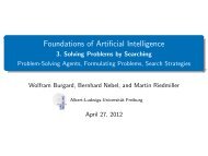
Fig. 3. The average RMS localization error and the success rate of the
extended Monte Carlo localization with simultaneous parameter estimation
compared to the standard localization with previously learned parameters of
the motion model. The error bars indicate the 5% confidence intervals over
ten runs.
together and a third laterally mounted rear propeller for yaw
rotation. Four small, lightweight wide-angle sonar sensors
provide distance measurements to the environment, which
are probabilistically modeled as described in our previous
work [15]. The experimental indoor environment has an area
for flying of about 14×7 m 2 with a vertical space of 5 m and
was mapped from 3D laser scans using multi-level surface
maps [24]. To determine the localization error, we put visual
markers onto the floor, which allow us to accurately calculate
the pose of the vehicle using the camera integrated in the
gondola of the blimp [1].
In an extensive experiment of about 9 minutes of manually
operated flight the blimp covered a distance of about 180 m.
Since we did not use an IMU and the wide-angle sonar
sensors provide hardly any information about the orientation
of the blimp, the localization relies on an accurate prediction
of the motion model. As can be seen in Fig. 3, the Monte
Carlo localization with simultaneous estimation of initially
unknown parameters benefits from the improved proposal
distribution. It resulted in a significantly lower rotational
localization error compared to the results obtained using the
implementation with previously learned (see section IV) and
fixed parameters of the motion model. The estimate of the
parameter vector typically converged within the first minute
of the experiment. Although the dimensionality of the state
estimation problem was increased by the four parameters, the
localization success rate revealed that the number of particles
required to reliably localize the blimp is substantially smaller
using the simultaneous parameter estimation.
Furthermore, we tested our localization system with simultaneous
parameter estimation in a global localization
szenario with initially unknown pose and motion model
parameters. We carried out 10 runs with 5,000 particles
each. Whereas the pose estimate typically converged within
the first 10 seconds, it still took 1 minute to determine
the parameters. Based on these experiments we expect that
translational error [m]
rotational error [deg]
0.1
0.09
0.08
0.07
0.06
0.05
5
4.5
4
3.5
3
2.5
2
0 0.05 0.1 0.15 0.2 0.25 0.3
relative covariance bound
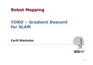
Fig. 4. The average translational and rotational RMS localization error
of a 10 minute localization experiment on simulation data. The error bars
indicate the 5% confidence intervals over ten runs.
our approach can also handle the kidnapped robot problem
given an extension which can distinguish between parameter
changes and kidnappings based on drops of the observation
likelihood.
B. Simulation of Changing Parameters
To evaluate the capability of our localization system to
adapt to changing parameters of the motion model, we
performed a series of experiments on a simulated blimp
using our deterministic motion model. The true poses were
passed as observations to the localization system and their
likelihood were modeled as a Gaussian distribution with high
translational and low rotational precision (σ trans = 0.2 m,
σ rot = 15 ◦ ).
In an experiment of about 10 minutes of manually operated
flight we evaluated different relative covariance bounds ρ in
our localization system using 5,000 particles. Note that we
experimentally tuned the parameters α short = 0.2, α long =
0.01, and ν = 0.8 to obtain best results. Although we
introduced only little noise to the velocity of the blimp during
simulation, the parameter estimation during localization was
a challenging task due to the correlation of the different
parameters (see Fig. 5). Furthermore, estimating all parameters
requires a certain spectrum of movements. For example,
during the first seconds of our experiment the blimp was
controlled to move forward only which resulted in a quick
convergence of solely the drag coefficient D x .
Fig. 4 presents the localization accuracy on the simulated
data during which the parameters of the motion model were
changed as depicted in Fig. 5. Both, the translational and
rotational localization error are significantly lower for a
relative covariance bound of ρ > 0.15 than without a lower
bound (ρ = 0) of the covariance of the parameters.
VI. CONCLUSIONS
In this paper, we presented a novel approach to Monte
Carlo localization of autonomous robots with simultaneous
estimation of the parameters of the motion model. In
contrast to other approaches, our systems allows an online
localization without prior knowledge of all motion model
parameters and can adapt to changed parameters during
operation. To avoid oscillations after parameter changes on
systems, for which these changes can only be detected with a

20
15
10
5
0
2
1.5
1
0.5
0
4
3.5
3
2.5
2
1.5
1
0.5
0
0.5
0.4
0.3
0.2
0.1
0
fin drag coefficient
real value
x drag coefficient
real value
y/z drag coefficient
real value
yaw drag coefficient
real value
0 100 200 300 400 500 600
time [s]
20
15
10
5
0
2
1.5
1
0.5
0
4
3.5
3
2.5
2
1.5
1
0.5
0
0.5
0.4
0.3
0.2
0.1
0
fin drag coefficient
real value
x drag coefficient
real value
y/z drag coefficient
real value
yaw drag coefficient
real value
0 100 200 300 400 500 600
time [s]
Fig. 5. The parameter estimation of exemplary localization runs of the simulated blimp without covariance bounding (left) and with ρ = 0.2 (right). The
area between the 2.5% and 97.5% quantiles of the estimated posterior is marked gray.
certain delay, our approach includes an appropriate damping
mechanism. In experiments carried out with a real blimp and
in simulation, we demonstrated that our system significantly
outperforms the standard Monte Carlo localization with
previously learned parameters in terms of the localization
accuracy and the number of particles needed.
REFERENCES
[1] M. Billinghurst and H. Kato. Collaborative augmented reality. Communications
of the ACM, (7), 2002.
[2] M. Bryson and S. Sukkarieh. Vehicle model aided inertial navigation
for a UAV using low-cost sensors. InProc.oftheAustralasianConf.on
Robotics & Automation (ACRA), 2004.
[3] F. Dellaert, D. Fox, W. Burgard, and W. Thrun. Monte carlo
localization for mobile robots. In Proc. of the IEEE Int. Conf. on
Robotics & Automation (ICRA), 1999.
[4] A. Doucet. On sequential simulation-based methods for bayesian filtering.
Technical report, Signal Processing Group, Dept. of Engeneering,
University of Cambridge, 1998.
[5] A.I. Eliazar and R. Parr. Learning probabilistic motion models for
mobile robots. In Proc. of the Int. Conf. on Machine Learning, 2004.
[6] G. Grisetti, C. Stachniss, and W. Burgard. Improving grid-based
slam with rao-blackwellized particle filters by adaptive proposals and
selective resampling. In Proc. of the IEEE Int. Conf. on Robotics &
Automation (ICRA), 2005.
[7] S. Grzonka, G. Grisetti, and W. Burgard. Towards a navigation system
for autonomous indoor flying. In Proc. of the IEEE Int. Conf. on
Robotics & Automation (ICRA), 2009.
[8] J.-S. Gutmann and D. Fox. An experimental comparison of localization
methods continued. In Proc. of the IEEE/RSJ Int. Conf. on Intelligent
Robots and Systems (IROS), Lausanne, Switzerland, 2002.
[9] R. He, S. Prentice, and N. Roy. Planning in information space for
a quadrotor helicopter in a gps-denied environments. In Proc. of the
IEEE Int. Conf. on Robotics & Automation (ICRA), 2008.
[10] A. Kaboli, M. Bowling, and P. Musilek. Bayesian calibration for
monte carlo localization. In Proc. of the National Conf. on Artificial
Intelligence (AAAI), 2006.
[11] J. Ko, D.J. Klein, D. Fox, and D. Haehnel. GP-UKF: Unscented
kalman filters with gaussian process prediction and observation models.
In Proc. of the IEEE/RSJ Int. Conf. on Intelligent Robots and
Systems (IROS), 2007.
[12] J. Liu and M. West. Combined parameter and state estimation in
simulation-based filtering. In Arnaud Doucet, Nando de Freitas, and
Neil Gordon, editors, Sequential Monte Carlo Methods in Practice,
chapter 10. 2001.
[13] J.S. Liu. Metropolized independent sampling with comparisons to
rejection sampling and importance sampling. Statist.Comput., 6, 1996.
[14] A. Martinelli, N. Tomatis, A. Tapus, and R. Siegwart. Simultaneous
localization and odometry calibration for mobile robot. In Proc. of the
IEEE/RSJ Int. Conf. on Intelligent Robots and Systems (IROS), 2003.
[15] J. Müller, A. Rottmann, and W. Burgard. A probabilistic sonar
sensor model for robust localization of a small-size blimp in indoor
environments using a particle filter. In Proc. of the IEEE Int. Conf. on
Robotics & Automation (ICRA), 2009.
[16] C. Plagemann and W. Burgard. Sequential parameter estimation for
fault diagnosis in mobile robots using particle filters. In Autonome
Mobile Systeme 2005 (AMS). Springer, 2005.
[17] C. Plagemann, C. Stachniss, and W. Burgard. Efficient failure detection
for mobile robots using mixed-abstraction particle filters. In H.I.
Christensen, editor, European Robotics Symposium 2006, volume 22
of STAR Springer tracts in advanced robotics. Springer Verlag, 2006.
[18] A. Rottmann, C. Plagemann, P Hilgers, and W. Burgard. Autonomous
blimp control using model-free reinforcement learning in a continuous
state and action space. In Proc. of the IEEE/RSJ Int. Conf. on
Intelligent Robots and Systems (IROS), 2007.
[19] A. Rottmann, M. Sippel, T. Ziterell, W. Burgard, L. Reindl, and
C. Scholl. Towards an experimental autonomous blimp platform. In
Proc. of the European Conf. on Mobile Robots (ECMR), 2007.
[20] N. Roy and S. Thrun. Online self-calibration for mobile robots. In
Proc. of the IEEE Int. Conf. on Robotics & Automation (ICRA), 1999.
[21] B. Steder, G. Grisetti, S. Grzonka, C. Stachniss, A. Rottmann, and
W. Burgard. Learning maps in 3d using attitude and noisy vision
sensors. In Proc. of the IEEE/RSJ Int. Conf. on Intelligent Robots and
Systems (IROS), 2007.
[22] S. Thrun, W. Burgard, and D. Fox. Probabilistic Robotics. MIT Press,
2005.
[23] S. Thrun, D. Fox, and W. Burgard. Monte carlo localization with
mixture proposal distribution. In Proc. of the National Conf. on
Artificial Intelligence (AAAI), 2000.
[24] R. Triebel, P. Pfaff, and W. Burgard. Multi-level surface maps for
outdoor terrain mapping and loop closing. In Proc. of the IEEE/RSJ
Int. Conf. on Intelligent Robots and Systems (IROS), 2006.
[25] J.C. Zufferey, A. Guanella, A. Beyeler, and D. Floreano. Flying over
the reality gap: From simulated to real indoor airships. Autonomous
Robots, 21(3), 2006.