HOROSPHERES IN HYPERBOLIC GEOMETRY 1. Introduction ...
HOROSPHERES IN HYPERBOLIC GEOMETRY 1. Introduction ...
HOROSPHERES IN HYPERBOLIC GEOMETRY 1. Introduction ...

Create successful ePaper yourself
Turn your PDF publications into a flip-book with our unique Google optimized e-Paper software.
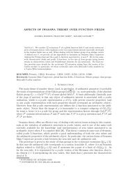
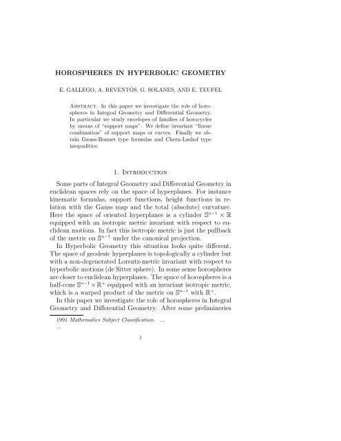
<strong>HOROSPHERES</strong> <strong>IN</strong> <strong>HYPERBOLIC</strong> <strong>GEOMETRY</strong><br />
E. GALLEGO, A. REVENTÓS, G. SOLANES, AND E. TEUFEL<br />
Abstract. In this paper we investigate the role of horospheres<br />
in Integral Geometry and Differential Geometry.<br />
In particular we study envelopes of families of horocycles<br />
by means of “support maps”. We define invariant “linear<br />
combination” of support maps or curves. Finally we obtain<br />
Gauss-Bonnet type formulas and Chern-Lashof type<br />
inequalities.<br />
<strong>1.</strong> <strong>Introduction</strong><br />
Some parts of Integral Geometry and Differential Geometry in<br />
euclidean spaces rely on the space of hyperplanes. For instance<br />
kinematic formulas, support functions, height functions in relation<br />
with the Gauss map and the total (absolute) curvature.<br />
Here the space of oriented hyperplanes is a cylinder S n−1 × R<br />
equipped with an isotropic metric invariant with respect to euclidean<br />
motions. In fact this isotropic metric is just the pullback<br />
of the metric on S n−1 under the canonical projection.<br />
In Hyperbolic Geometry this situation looks quite different.<br />
The space of geodesic hyperplanes is topologically a cylinder but<br />
with a non-degenerated Lorentz-metric invariant with respect to<br />
hyperbolic motions (de Sitter sphere). In some sense horospheres<br />
are closer to euclidean hyperplanes. The space of horospheres is a<br />
half-cone S n−1 ×R + equipped with an invariant isotropic metric,<br />
which is a warped product of the metric on S n−1 with R + .<br />
In this paper we investigate the role of horospheres in Integral<br />
Geometry and Differential Geometry. After some prelimineries<br />
1991 Mathematics Subject Classification. ...<br />
...<br />
1
2 E. GALLEGO, A. REVENTÓS, G. SOLANES, AND E. TEUFEL<br />
we study in section 3 envelopes of families of horocycles by means<br />
of “support maps”. In section 4 we define invariant “linear combination”<br />
of support maps or curves. Finally in section we<br />
obtain Gauss-Bonnet type formulas and Chern-Lashof type inequalities.<br />
This work was done when the fourth author was visitor at the<br />
CRM within the research programm “Geometric Flows. Equivariant<br />
Problems in Symplectic Geometry”.<br />
2. Preliminaries<br />
We use the Lorentz space model for the Hyperbolic Geometry.<br />
In detail, the model lives in Lorentz space R n+1<br />
1 with its Lorentz<br />
product<br />
〈x, y〉 = x 1 y 1 + x 2 y 2 + · · · + x n y n − x n+1 y n+1 .<br />
The n-dimensional hyperbolic space H n is realized as<br />
H n = {x ∈ R n+1<br />
1 : 〈x, x〉 = −1 ∧ x n+1 > 0}<br />
i.e. the upper half of an two-sheeted hyperboloid with the light<br />
cone C n = {x ∈ R n+1<br />
1 : 〈x, x〉 = 0} as asymptotic cone. The<br />
group G of hyperbolic motions of H n is given by the subgroup<br />
of the Lorentz group leaving invariant H n .<br />
The space H of horospheres of H n is realized as the upper half<br />
of the light cone, i.e.<br />
H = C n +<br />
= {x ∈ Rn+1 1 : 〈x, x〉 = 0 ∧ x n+1 > 0 .}<br />
Indeed, horospheres in H n are exactly the non-void sections of<br />
H n with hyperplanes which are parallel to hyperplanes tangent<br />
to the light cone C n . Given θ ∈ C+ n , then the affine hyperplane<br />
Θ = {x ∈ R n+1<br />
1 : 〈x, θ〉 = −1} is parallel to the tangent hyperplane<br />
T θ C+ n = {x ∈ Rn+1 1 : 〈x, θ〉 = 0} of C+ n at θ and intersects<br />
H n in horosphere which we also denote by Θ. Given a horosphere<br />
Θ in H n , i.e. the intersection of H n with an affine hyperplane Θ<br />
parallel to a tangent hyperplane of C+ n along along a half lightray.<br />
Then there exists exactly one θ in this half light-ray such<br />
that Θ = {x ∈ R n+1<br />
1 : 〈x, θ〉 = −1}. (In the following we shall
<strong>HOROSPHERES</strong> <strong>IN</strong> <strong>HYPERBOLIC</strong> <strong>GEOMETRY</strong> 3<br />
always denote horospheres in H n (or the underlying affine hyperplane)<br />
by capital greek letters and the vectors representing<br />
them in C+ n by the corresponding small greek letters.)<br />
The correspondence between θ and the hyperplane Θ comes<br />
exactly from the polarity relation with respect to the quadric<br />
±H n ⊂ R n+1<br />
1 . The Lorentz product induces on C n a degenerated<br />
product (isotropic metric).<br />
The light-rays in the cone C+ n are exactely the pencils of “parallel”<br />
horospheres. Two parallel horospheres Θ 1 and Θ 2 touch<br />
one another at a point at infinity, and they lie in constant hyperbolic<br />
distance to each other. A little computation in the model<br />
shows that this distance is given by | lnλ|, where λ ∈ R + is given<br />
by θ 2 = λθ 1 . Here we use the signed distance from Θ 1 to Θ 2 by<br />
d(Θ 1 , Θ 2 ) = − ln λ . (1)<br />
For fixed Θ 1 , as λ → +∞ the horosphere Θ 2 shrinks to the common<br />
point at infinity whereas the signed distance d(Θ 1 , Θ 2 ) →<br />
−∞. On the other side, if λ → 0, then Θ 2 expands over the<br />
whole H n and d(Θ 1 , Θ 2 ) → +∞.<br />
The space of horospheres H = C+ n ⊂ Rn+1 1 is endowed with a<br />
n-form ω which is invariant under the Lorentz group. In terms<br />
of the coordinates (x 1 , . . ., x n+1 ) ∈ R n+1<br />
1 this form is given by<br />
ω = 1<br />
x n+1<br />
dx 1 ∧ . . . ∧ dx n+1 = x n−2<br />
n+1dx n+1 dv (2)<br />
where dv is the spherical volume element at x −1<br />
n+1 (x 1, . . .,x n ) ∈<br />
S n−1 , cf. [San67], [San68].<br />
Our bridge between the point space H n and the space of horospheres<br />
C+ n is the following.<br />
Definition 2.<strong>1.</strong> Let M be a smooth regular hypersurface in H n<br />
and ν(x), x ∈ M, a unit normal vector field along M. Then<br />
θ(x) = x + ν(x) ∈ C+ n represents the horosphere Θ(x) which is<br />
tangent to M at x such that ν(x) points into its convex side. We<br />
call<br />
θ : M −→ C+ n , x ↦→ x + ν(x) (3)
4 E. GALLEGO, A. REVENTÓS, G. SOLANES, AND E. TEUFEL<br />
the “support map” of M.<br />
The support map θ of M is smooth, and in general tranverse<br />
to the generators of C n + .<br />
3. Envelopes of horocycles<br />
3.<strong>1.</strong> Support maps: from c to θ. Let us start with a regular<br />
parametrized curve c(s) in H 2 , s ∈ I , s an arc length parameter.<br />
In order to describe the differential geometry of the curve, we<br />
use the Frenet theory. That means we have the positive oriented<br />
Frenet frame along c, build by the unit tangent vector<br />
e 1 (s) = c ′ (s) and the normal unit vector e 2 (s). The Frenet equations<br />
▽ e1 (s)e 1 (s) = κ g (s)e 2 (s), ▽ e1 (s)e 2 (s) = −κ g (s)e 1 (s) then<br />
define the geodesic curvature κ g of c (▽ denotes the co-variant<br />
derivative in H 2 ).<br />
In order to describe the support map, let ν(s) be a unit normal<br />
vector field along c. We consider the support map θ of c with<br />
respect to ν, i.e.<br />
θ : I → C 2 +<br />
with θ(s) = c(s) + ν(s).<br />
The horocycle Θ(s) is tangent to c at c(s) and ν(s) points into<br />
its convex side.<br />
Then (the primes denote derivations with respect to s)<br />
θ ′ = c ′ + ν ′ = c ′ + ǫe ′ 2 = (1 − ǫκ g)e 1<br />
with ǫ := 〈ν, e 2 〉. (Note: 〈e 2 , e 2 〉 = 1 ⇒ 〈e 2 , e ′ 2〉 = 0 , 〈c, e 2 〉 =<br />
0 ⇒ 0 = 〈c ′ , e 2 〉 + 〈c, e ′ 2 〉 = 〈c, e′ 2 〉, hence e′ 2 ∈ T cH 2 .)<br />
this shows that the curve θ(s) is regular parametrized iff κ g ≠ ǫ<strong>1.</strong><br />
The curve θ(s) is then space-like, and its arc length parameter<br />
σ is given by<br />
dσ = |1 − ǫκ g |ds. (4)<br />
3.2. Envelopes: from θ to c. Let us start with a regular<br />
parametrized curve θ(σ) in C+ 2 which is locally a graph with respect<br />
to the generators of C+ 2 , σ ∈ I, σ an arc length parameter,
<strong>HOROSPHERES</strong> <strong>IN</strong> <strong>HYPERBOLIC</strong> <strong>GEOMETRY</strong> 5<br />
i.e 〈 ˙θ, ˙θ〉 = <strong>1.</strong> We look for the envelope curve c(σ) of the family<br />
Θ(σ) of horocycles in H 2 , i.e.<br />
〈c, c〉 = −1,<br />
〈c, θ〉 = −1, (5)<br />
〈ċ, θ〉<br />
= 0 (envelope condition).<br />
For the curve θ we have<br />
〈θ, θ〉 = 0 ⇒ 〈 ˙θ, θ〉 = 0 ⇒ 0 = 〈¨θ, θ〉 + 〈 ˙θ, ˙θ〉 = 〈¨θ, θ〉 + 1<br />
(the points denote derivations with respect to σ),<br />
〈 ˙θ, ˙θ〉 = 1 ⇒ 〈 ˙θ, ¨θ〉 = 0 , and<br />
〈 ˙θ, ¨θ〉 = 0 ⇒ 〈¨θ, ¨θ〉 ...<br />
+ 〈 ˙θ, θ 〉 = 0 .<br />
From (5) we get<br />
〈c, c〉 = −1 ⇒ 〈ċ, c〉 = 0 , and<br />
〈c, θ〉 = −1 ⇒ 0 = 〈ċ, θ〉 + 〈c, ˙θ〉 = 〈c, ˙θ〉.<br />
Now, we assume that θ, ˙θ, ¨θ are linear independent, and we try<br />
c = αθ + β ˙θ + γ¨θ with unknown functions α, β, γ . We take into<br />
account the above relations, i.e.<br />
0 = 〈c, ˙θ〉 = α〈θ, ˙θ〉 + β〈 ˙θ, ˙θ〉 + γ〈¨θ, ˙θ〉 = β , and<br />
−1 = 〈c, θ〉 = α〈θ, θ〉 + β〈 ˙θ, θ〉 + γ〈¨θ, θ〉 = −γ , and<br />
−1 = 〈c, c〉 = α 2 〈θ, θ〉+β 2 〈 ˙θ, ˙θ〉+γ 2 〈¨θ, ¨θ〉+2αβ〈θ, ˙θ〉+2αγ〈θ, ¨θ〉+<br />
2βγ〈 ˙θ, ¨θ〉 = γ 2 〈¨θ, ¨θ〉 − 2αγ .<br />
And we get<br />
c = 1 (<br />
1 + 〈¨θ,<br />
2<br />
¨θ〉<br />
)<br />
θ + ¨θ . (6)<br />
Now, with the expression (6) for c we directly check<br />
〈c, c〉 = −1 , i.e. c ⊂ H n , 〈c, θ〉 = −1 , i.e. c ∈ Θ , and 〈ċ, θ〉 = 0.<br />
And therefore, c is the envelope of Θ we looked for.<br />
From (6) we get by differentiation<br />
1 − 〈¨θ, ¨θ〉<br />
ċ = ˙θ . (7)<br />
2<br />
(To this, we try ...<br />
θ as a linear combination of the vectors θ, ˙θ, ¨θ.<br />
We take into account 〈¨θ, θ〉 = −1 ⇒ 〈¨θ, ˙θ〉 + 〈 ...<br />
θ , θ〉 = 0 and<br />
〈¨θ, ˙θ〉 = 0 ⇒ 〈¨θ, ¨θ〉 + 〈 ...<br />
θ , ˙θ〉 = 0, in order to get ...<br />
θ = −〈 ...<br />
θ , ¨θ〉θ −
6 E. GALLEGO, A. REVENTÓS, G. SOLANES, AND E. TEUFEL<br />
〈¨θ, ¨θ〉 ˙θ.)<br />
Formula (7) shows that the envelope c is regular iff 〈¨θ, ¨θ〉 ≠ <strong>1.</strong><br />
Remark 3.<strong>1.</strong> The condition 〈¨θ, ¨θ〉 ≠ 1 means, that the osculating<br />
plane of the curve θ in R 3 1 is not tangent to the model H 2 .<br />
This property characterizes curves θ in C+ 2 which envelope regular<br />
curves in H 2 .<br />
Remark 3.2. The osculating plane of θ at a fixed parameter defines<br />
a family of horocycles with the following geometric meaning:<br />
If the osculating plane is space-like, then the envelope curve<br />
c of θ has an osculating circle at the point under consideration.<br />
We have |κ g | > 1 at this point. And the family of horocycles<br />
envelopes this osculating circle on their concave sides or convex<br />
sides respectively, if the plane of the family intersects H 2 or<br />
avoids H 2 respectively.<br />
If the osculating plane is of mixed type, then the envelope curve<br />
c of θ has an osculating equidistant at the point under consideration.<br />
We have |κ g | < 1 at this point. And the family of<br />
horocycles envelopes this equidistant.<br />
Finally we compute the geodesic curvature κ g of the curve c<br />
in terms of θ:<br />
From (6) we have c = αθ + γ¨θ, and further<br />
c ′ = dc<br />
ds = dσ<br />
dsċ = dσ<br />
ds<br />
(<br />
˙αθ + α ˙θ + ˙γ¨θ + γ ...<br />
θ<br />
Because of c ′ ∼ ˙θ and | ˙θ| = 1 we can compute<br />
1 = |c ′ | = |〈c ′ , ˙θ〉| 〈<br />
= |1 − ǫκ g | ∣ ˙αθ + α ˙θ + ˙γ¨θ + γ ... ˙θ〉∣ ∣∣<br />
θ , =<br />
(<br />
= |1 − ǫκ g | ∣ ˙α〈θ, ˙θ〉 + α〈 ˙θ, ˙θ〉 + ˙γ〈¨θ, ˙θ〉 + γ〈 ... ˙θ〉)∣ ∣∣<br />
θ , =<br />
(<br />
¨θ〉)∣ ∣∣<br />
= |1 − ǫκ g | ∣ α − γ〈¨θ, .<br />
Inserting the coefficients α, β from (6) we get<br />
1 = |1 − ǫκ (<br />
g|<br />
¨θ〉)∣ ∣∣<br />
∣ 1 − 〈¨θ, . (8)<br />
2<br />
)<br />
.
<strong>HOROSPHERES</strong> <strong>IN</strong> <strong>HYPERBOLIC</strong> <strong>GEOMETRY</strong> 7<br />
3.3. Further relations between c and θ. We want to write<br />
the length L(c) and the total curvature TC(c) of the point curve<br />
c in terms of the support curve θ.<br />
Proposition 3.<strong>1.</strong> Let c(s), s ∈ I, be a regular curve in H 2<br />
parametrized by arc length s and ν(s) a unit normal vector field<br />
along c. Let θ : I → C+ 2 , θ(s) = c(s) + ν(s) denote the support<br />
map of c with respect to ν, and set ǫ = 〈ν, e 2 〉.<br />
If ǫ = +1 and κ g > 1, or ǫ = −1 and κ g > −1 respectively, then<br />
L(c) = 1 ∫<br />
ǫ ( κ 2 θ<br />
2<br />
− 1) dσ, (9)<br />
θ<br />
where κ θ is the curvature of the curve θ as a curve in R 3 1, and<br />
∫<br />
TC(c) = κ g ds = 1 ∫<br />
(<br />
κ<br />
2<br />
c 2 θ + 1 ) dσ. (10)<br />
Proof. The case ǫ = +1 and κ g > 1: From (4) and (8) we get<br />
ds = 1 |1 − 〈¨θ, ¨θ〉|<br />
dσ = dσ.<br />
κ g − 1 2<br />
Locally c lies in the convex side of Θ, hence we have 〈c, ¨θ〉 > 0.<br />
(This can be seen in the model: Take the intersection of C+<br />
2<br />
and the plane through θ in direction span( ˙θ, ¨θ) which represents<br />
the horocycles tangent to the osculating circle of c, and take<br />
into account that c locally lies in the convex side of Θ.) Hence<br />
through (6) we have 1 − 〈¨θ, ¨θ〉 < 0. Because σ is an arc length<br />
parameter on θ we have 〈¨θ, ¨θ〉 = κ 2 θ . Altogether we get (9).<br />
From (4) and (8), taking into account 1 − 〈¨θ, ¨θ〉 < 0, we get<br />
θ<br />
κ θ ds = 〈¨θ, ¨θ〉 + 1<br />
2<br />
dσ,<br />
hence we get (10).<br />
In case ǫ = −1 and κ g > −1 the proof runs analogously.<br />
□
8 E. GALLEGO, A. REVENTÓS, G. SOLANES, AND E. TEUFEL<br />
4. Linear combinations of support maps<br />
In the cone C n + each generator is a half-ray, i.e. R+ . Hence<br />
along each generator we have an addition and a multiplication,<br />
as far as well defined. This way we are able to define “linear<br />
combinations” of support maps. In the following we investigate<br />
the 2-dimensional situation.<br />
4.<strong>1.</strong> The “λ-multiple”.<br />
Definition 4.<strong>1.</strong> Let c(s), s ∈ I, be a regular curve in H 2 parametrized<br />
by arc length s and ν(s) a unit normal vector field along c. Let<br />
θ : I → C+ 2 , θ(s) = c(s) + ν(s) denote the support map of c with<br />
respect to ν.<br />
For λ ∈ R + , we call the envelope of λθ in H n , in case it is well<br />
defined, the “λ-multiple λ c of c”.<br />
We consider the case ǫ = +1 and κ g > <strong>1.</strong> Then locally c lies<br />
in the convex side of each of its tangent horocycles which are<br />
supporting c, and we have 〈¨θ, ¨θ〉 > <strong>1.</strong><br />
We consider θ ∗ = λθ with λ > 0. Using (1) we set t = d(Θ, Θ ∗ ) =<br />
− ln λ.<br />
a) The case λ > 1: The envelope c ∗ of θ ∗ is the inner parallel<br />
curve to c at distance t.<br />
We compute<br />
〈 d2 θ ∗ d 2 θ ∗<br />
(dσ ∗ ) 2, (dσ ∗ ) 〉 = 1 2 λ 〈¨θ, ¨θ〉 .<br />
2<br />
Taking into account (7) we get: If λ 2 < 〈¨θ, ¨θ〉 = κ 2 θ , then the<br />
envelope c ∗ is regular. Singular points occur for λ 2 = 〈¨θ, ¨θ〉.<br />
In our case we have 〈¨θ, ¨θ〉 > <strong>1.</strong> Therefore (8) implies<br />
κ g = 〈¨θ, ¨θ〉 + 1<br />
〈¨θ, ¨θ〉 − 1 . (11)<br />
The geodesic curvature κ g and the curvature radius ρ are related<br />
by<br />
κ g = coth ρ = e2ρ + 1<br />
e 2ρ − 1 , (12)
<strong>HOROSPHERES</strong> <strong>IN</strong> <strong>HYPERBOLIC</strong> <strong>GEOMETRY</strong> 9<br />
hence<br />
e 2ρ = 〈¨θ, ¨θ〉 . (13)<br />
This shows that singular points occur for t = −ρ, i.e. singular<br />
points occur when the inner parallel curve of c runs through focal<br />
points of c.<br />
b) The case λ < 1: The envelope c ∗ = c t of θ ∗ is the outer<br />
parallel curve to c at distance t.<br />
Because of λ < 1, formula (7) shows that c t is regular for all<br />
t > 0.<br />
We now compute the length of c t : Using (9), dσ ∗ = λ dσ, we get<br />
L(c t ) = L(c ∗ ) = 1 〈<br />
2<br />
∫θ d2 θ ∗ d 2 θ ∗<br />
(dσ ∗ ∗ ) 2, (dσ ∗ ) 〉 2 dσ∗ − 1 ∫<br />
dσ ∗ =<br />
2 θ ∗<br />
= 1 ∫<br />
1<br />
〈¨θ,<br />
2 λ<br />
¨θ〉 dσ − 1 ∫<br />
θ 2 λ dσ =<br />
θ<br />
= 1 ( ) ∫ 1<br />
2 λ − λ κ g ds + 1 ( ) 1<br />
c 2 λ + λ L(c) .<br />
And replacing λ = e −t , we arrive at<br />
∫<br />
L(c t ) = sinh(t) κ g ds + cosh(t)L(c) . (14)<br />
c<br />
This is a well-known Steiner formula in hyperbolic plane, cf. e.g.<br />
[San76].<br />
4.2. The “sum”.<br />
Definition 4.2. Let c 1 , c 2 be two regular curves in H 2 and θ 1 , θ 2<br />
their support maps with respect to unit normal fields ν 1 , ν 2 along<br />
c 1 , c 2 . Then we call the envelope of θ 1 + θ 2 in H n , in case it is<br />
well defined, the “sum c 1 + c 2 of c 1 and c 2 ”.<br />
Suppose θ 2 = λθ 1 , parametrized by the arc length parameter<br />
σ 1 on θ 1 . Then we have<br />
dθ 2<br />
= dλ θ 1 + λ dθ 1<br />
,<br />
dσ 1 dσ 1 dσ 1<br />
〈 dθ 2<br />
dσ 1<br />
, dθ 2<br />
dσ 1<br />
〉 = λ 2 〈 dθ 1<br />
dσ 1<br />
, dθ 1<br />
dσ 1<br />
〉 = λ 2 ,
10 E. GALLEGO, A. REVENTÓS, G. SOLANES, AND E. TEUFEL<br />
hence<br />
dσ 2 = λ dσ 1 . (15)<br />
We consider, in case it is well defined, θ ∗ = θ 1 + θ 2 = (1 + λ) θ 1 .<br />
Then we have<br />
dθ ∗<br />
= dλ θ 1 + (1 + λ) dθ 1<br />
dσ 1 dσ 1 dσ 1<br />
and<br />
〈 dθ∗ , dθ∗ 〉 = (1 + λ) 2 〈 dθ 1<br />
, dθ 1<br />
〉 = (1 + λ) 2 .<br />
dσ 1 dσ 1 dσ 1 dσ 1<br />
Therefore we get<br />
dσ ∗ = (1 + λ) dσ 1 = 1 + λ<br />
λ dσ 2 = dσ 1 + dσ 2 , (16)<br />
and we arrive at<br />
Proposition 4.<strong>1.</strong> For the lengths of the support images involved<br />
in the “sum” the following relation holds<br />
L(θ ∗ ) = L(θ 1 + θ 2 ) = L(θ 1 ) + L(θ 2 ) . (17)<br />
In order to compute the length L ∗ and the total curvature TC ∗<br />
of the sum in terms of the summands, we need the following<br />
Definition 4.3. Let c 1 , c 2 be two regular curves in H 2 and θ 1 , θ 2<br />
their support maps with respect to unit normal fields ν 1 , ν 2 along<br />
c 1 , c 2 . Then θ 2 = λθ 1 , and the signed distance d(Θ 1 , Θ 2 ) from<br />
Θ 1 to Θ 2 is given by d(Θ 1 , Θ 2 ) = − ln λ , cf. (1). We call<br />
w 12 : θ 1 → R , σ 1 ↦→ − ln λ(σ 1 ) (18)<br />
the “mixed width function of c 1 and c 2 with respect to c 1 ”.<br />
The mixed width function describes the relative position of c 1<br />
and c 2 to one another in terms of the distance between parallel<br />
tangent horocycles.<br />
Remark 4.<strong>1.</strong> If θ 1 is the support map of a point O ∈ H 2 , then<br />
w 12 coincides with the horocycle support function of c 2 based at<br />
the point O, cf. [Fil70], [San67], [San68].
<strong>HOROSPHERES</strong> <strong>IN</strong> <strong>HYPERBOLIC</strong> <strong>GEOMETRY</strong> 11<br />
Remark 4.2. If c 1 = c 2 = c and c is h-convex, then the mixed<br />
width function w 12 coincides with the width function with respect<br />
to horocycles considered in [].<br />
4.2.<strong>1.</strong> The sum of “concave-sided” support maps. We consider<br />
the following situation: Let c 1 , c 2 be two regular curves in H 2<br />
with geodesic curvatures (κ g ) 1 , (κ g ) 2 > −<strong>1.</strong> We take the support<br />
maps θ 1 , θ 2 according to ǫ 1 = ǫ 2 = −1, that means locally<br />
the curves lie on the concave sides of their respective support<br />
horocycles.<br />
Proposition 4.2. Suppose the situation described above. Then,<br />
whenever well defined, the sum θ ∗ = θ 1 + θ 2 envelopes a regular<br />
curve c ∗ = c 1 + c 2 in H 2 with<br />
(i) κ ∗ g > −1 , and<br />
(ii) c ∗ lies locally on the concave sides of its respective support<br />
horocycles.<br />
Proof. The curves c 1 , c 2 lie locally on the concave sides of their<br />
respective support horocycles, therefore the osculating planes of<br />
θ 1 , θ 2 intersect H 2 without being tangent (cf. Remark 3.1).<br />
Now, we keep fixed an arbitrary parameter σ 1 .<br />
The osculating plane of θ 1 at σ 1 is given by<br />
θ 1 (σ 1 ) + span( ˙θ 1 (σ 1 ), ¨θ 1 (σ 1 )).<br />
Let P 1 denote the parallel plane through θ ∗ (σ 1 ), i.e.<br />
P 1 = θ ∗ (σ 1 ) + span( ˙θ 1 (σ 1 ), ¨θ 1 (σ 1 )).<br />
The osculating plane of θ 1 at σ 1 intersects H 2 without being<br />
tangent, and θ ∗ = θ 1 +θ 2 , therefore P 1 also intersects H 2 without<br />
being tangent.<br />
Now θ 2 = λθ 1 , hence<br />
θ˙<br />
2 = ˙λθ 1 + λθ ˙ 1 and ¨θ2 = ¨λθ 1 + 2˙λ θ ˙ 1 + λ ¨θ 1 (19)<br />
(where the dots denote derivatives with respect to σ 1 ). And the<br />
osculating plane of θ 2 at σ 1 is given by<br />
θ 2 (σ 1 ) + span( ˙θ 2 (σ 1 ), ¨θ 2 (σ 1 )).
12 E. GALLEGO, A. REVENTÓS, G. SOLANES, AND E. TEUFEL<br />
Let P 2 denote the parallel plane through θ ∗ (σ 1 ), i.e.<br />
P 2 = θ ∗ (σ 1 ) + span( ˙θ 2 (σ 1 ), ¨θ 2 (σ 1 )).<br />
The osculating plane of θ 2 at σ 1 intersects H 2 without being<br />
tangent, we have θ ∗ = θ 1 + θ 2 , therefore P 2 also intersects H 2<br />
without being tangent.<br />
The osculating plane of θ ∗ at σ 1 is given by<br />
with<br />
P ∗ = θ ∗ (σ 1 ) + span( ˙θ ∗ (σ 1 ), ¨θ ∗ (σ 1 ))<br />
˙θ ∗ = ˙θ 2 + ˙θ 1 and ¨θ ∗ = ¨θ 2 + ¨θ 1 . (20)<br />
Let T be the tangent plane of C 2 + along the generator R + ·θ 1 (σ 1 ),<br />
i.e.<br />
T = θ ∗ (σ 1 ) + span(θ 1 (σ 1 ), ˙θ 1 (σ 1 )). For a ≥ 0 let T a denote the<br />
plane parallel to T given by T a = T + a ¨θ 1 (σ 1 ).<br />
Then T a intersects P 1 in the line<br />
l 1a = θ ∗ (σ 1 ) + a ¨θ 1 (σ 1 ) + R · ˙θ 1 (σ 1 ) .<br />
And by (19), T a intersects P 2 in the line<br />
l 2a = θ ∗ (σ 1 ) +<br />
a<br />
λ(σ 1 ) ¨θ 2 (σ 1 ) + R · ˙θ 2 (σ 1 ) .<br />
And by (20), T a intersects P ∗ in the line<br />
l ∗ a = a<br />
θ∗ (σ 1 )+<br />
(¨θ2 (σ 1 ) +<br />
1 + λ(σ 1 )<br />
¨θ 1 (σ 1 ))<br />
+R·(<br />
˙θ2 (σ 1 ) + ˙θ<br />
)<br />
1 (σ 1 ) .<br />
Let g a denote the line in T a given by<br />
g a = θ ∗ (σ 1 ) + a ¨θ 1 (σ 1 ) + R · θ 1 (σ 1 ) .<br />
Then g a intersects l 1a in the point<br />
Q 1a = θ ∗ (σ 1 ) + a ¨θ 1 (σ 1 ) .<br />
And g a intersects l 2a in the point<br />
Q 2a = θ ∗ (σ 1 ) + a ¨θ 1 (σ 1 ) + a(λ¨λ − 2˙λ 2 )<br />
λ 2 | σ1 θ 1 (σ 1 ) .
<strong>HOROSPHERES</strong> <strong>IN</strong> <strong>HYPERBOLIC</strong> <strong>GEOMETRY</strong> 13<br />
And g a intersects l ∗ a in the point<br />
Q ∗ a = θ∗ (σ 1 ) + a ¨θ 1 (σ 1 ) + a((1 + λ)¨λ − 2˙λ 2 )<br />
(1 + λ) 2 | σ1 θ 1 (σ 1 ) .<br />
The proof now splits into two cases.<br />
The first case, ((1 + λ)¨λ − 2˙λ 2 )| σ1 ≥ 0:<br />
P 1 intersects H 2 without being tangent. Therefore there exists an<br />
a > 0 such that l 1a intersects the parabola T a ∩H 2 without being<br />
tangent. The axis of the parabola is θ ∗ (σ 1 )+a ¨θ 1 (σ 1 )+R·θ 1 (σ 1 ).<br />
Hence the half-ray Q 1a +R +·θ 1 (σ 1 ) ⊂ T a lies in the convex region<br />
bounded by the parabola T a ∩ H 2 . In the first case Q ∗ a lies on<br />
this half-ray. Hence Q ∗ a lies in the convex region bounded by<br />
the parabola T a ∩ H 2 . Hence l ∗ a intersects the parabola T a ∩ H 2<br />
without being tangent. Hence the osculating plane P ∗ of θ ∗ at<br />
σ 1 intersects H 2 without being tangent.<br />
The second case, ((1 + λ)¨λ − 2˙λ 2 )| σ1 < 0:<br />
P 2 intersects H 2 without being tangent. Therefore there exists<br />
an a > 0 such that l 2a intersects the parabola T a ∩ H 2 without<br />
being tangent. Hence the half-ray Q 2a + R + · θ 1 (σ 1 ) ⊂ T a lies in<br />
the convex region bounded by the parabola T a ∩ H 2 . Through<br />
the assumption in the second case we have<br />
λ¨λ − 2˙λ 2<br />
λ 2 | σ1 ≤ (1 + λ)¨λ − 2˙λ 2<br />
(1 + λ) 2 | σ1 .<br />
Hence Q ∗ a lies on this half-ray. Hence l∗ a intersects the parabola<br />
T a ∩ H 2 without being tangent. Hence the osculating plane P ∗<br />
of θ ∗ at σ 1 intersects H 2 without being tangent.<br />
Altogether, this shows that the osculating planes of θ ∗ intersect<br />
H 2 without being tangent. Therefore c ∗ is regular at σ 1 , θ ∗ supports<br />
c ∗ concave-sided, and moreover κ ∗ g > −<strong>1.</strong> □<br />
Proposition 4.3. Suppose the situation described above. Then<br />
the length L ∗ and the total curvature TC ∗ of c ∗ = c 1 + c 2 write<br />
in terms of c 1 , c 2 and their relative position to each other in H 2
14 E. GALLEGO, A. REVENTÓS, G. SOLANES, AND E. TEUFEL<br />
as follows:<br />
L ∗ = − 1 2 (W(c 1, c 1 + c 2 ) − L 1 − TC 1 − L 2 − TC 2 ) (21)<br />
TC ∗ = 1 2 (W(c 1, c 1 + c 2 ) + L 1 + TC 1 + L 2 + TC 2 ) , (22)<br />
with<br />
∫<br />
W(c 1 , c 1 + c 2 ) = TC ∗ − L ∗ = e ( ) w 1∗<br />
(ẇ 1∗ ) 2 + 2ẅ 1∗ + κ 2 θ dσ1 1<br />
θ 1<br />
and the mixed with function<br />
w 1∗ (σ 1 ) = − ln(1 + λ(σ 1 )).<br />
Proof. By the assumptions on c 1 , c 2 and by Proposition 4.2 we<br />
have for all three curves c 1 , c 2 , c ∗ that ǫ 1 = ǫ 2 = ǫ ∗ = −1 and<br />
(κ g ) 1 , (κ g ) 2 , κ ∗ g > −<strong>1.</strong> Therfore (6) writes dσ = (κ g+1) ds, hence<br />
∫ ∫ ∫<br />
L(θ) = dσ = (κ g + 1) ds = κ g ds + L(c) . (23)<br />
This and (17) gives<br />
From (4) and (8) we get<br />
θ<br />
c<br />
TC ∗ + L ∗ = TC 1 + L 1 + TC 2 + L 2 . (24)<br />
ds =<br />
L(c) = − 1 2<br />
This applied to c ∗ yields<br />
L(c ∗ ) = − 1 2<br />
∫<br />
1 − 〈¨θ, ¨θ〉<br />
2<br />
∫<br />
θ<br />
dσ,<br />
κ 2 θ dσ + 1 2 L(θ).<br />
c<br />
θ ∗ κ 2 θ ∗ dσ∗ + 1 2 L(θ∗ ). (25)
<strong>HOROSPHERES</strong> <strong>IN</strong> <strong>HYPERBOLIC</strong> <strong>GEOMETRY</strong> 15<br />
Now a straightforward but lenghty computation, not acted out<br />
here, starts at θ ∗ = (1 + λ) θ 1 and reaches<br />
[ ( )<br />
〈 d2 θ ∗ d2 θ ∗<br />
2<br />
dσ ∗2, dσ 〉 = 1 d<br />
(ln(1 + λ)) −<br />
∗2 (1 + λ) 2 dσ 1<br />
]<br />
−2 d2<br />
(ln(1 + λ)) + 〈<br />
dσ ¨θ<br />
1<br />
2 1 , ¨θ 1 〉 . (26)<br />
Using the mixed with function of c 1 and c ∗ with respect to c 1 ,<br />
i.e. w 1∗ = − ln(1 + λ), formula (26) gives<br />
∫<br />
κ 2 θ ∗ dσ∗ = 〈<br />
θ<br />
∫θ d2 θ ∗ d2 θ ∗<br />
dσ ∗2, dσ 〉 ∗ ∗ ∗2 dσ∗ =<br />
∫<br />
= e ( ) w 1∗<br />
(ẇ 1∗ ) 2 + 2ẅ 1∗ + κ 2 θ dσ1 1<br />
. (27)<br />
θ 1<br />
(Note: dσ ∗ = (1 + λ) dσ 1 cf. (16).)<br />
Hence (25), (27) and (23) yield<br />
L ∗ = − 1 ∫<br />
e ( ) w 1∗<br />
(ẇ 1∗ ) 2 + 2ẅ 1∗ + κ 2 θ dσ1<br />
2<br />
1<br />
+ 1<br />
θ 1<br />
2 TC∗ + 1 2 L∗ . (28)<br />
Finally (24) and (28) give the result.<br />
□<br />
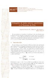
c 1<br />
c 2<br />
c 1 + c 2
16 E. GALLEGO, A. REVENTÓS, G. SOLANES, AND E. TEUFEL<br />
Figure 1: The sum c 1 + c 2 of two circles c 1, c 2 in the Poincaré disk, with radii<br />
r 1 = 1, r 2 = 0.5 and distance 2 between their centers<br />
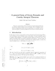
c 1 c 2<br />
c 1 + c 2<br />
Figure 2: The sum c 1 + c 2 of two circles c 1, c 2 in the Poincaré disk, with radii<br />
4.3. The “rum”.<br />
r 1 = 0.16, r 2 = 2 and distance 5 between their centers<br />
Definition 4.4. Let c 1 , c 2 be two regular curves and θ 1 , θ 2 their<br />
support maps with respect to unit normal fields ν 1 , ν 2 along c 1 , c 2 .<br />
Then θ 2 = λθ 1 . Whenever well-defined, we call<br />
c 1 #c 2 = c ∗ , given by θ ∗ = λ<br />
1 + λ θ 1 (29)<br />
the “rum c 1 #c 2 of c 1 and c 2 ”.<br />
Geometrically, this definition is induced by the sum of the two<br />
parallel planes Θ 1 and Θ 2 in the vector space R 3 1 .<br />
Lemma 4.<strong>1.</strong> Let θ 1 , θ 2 be support maps. Then θ ∗ = θ 1 #θ 2 lies<br />
below θ 1 and θ 2 with respect to each of the generators of C n + .<br />
Proof. This follows immediately from the geometric meaning of<br />
the definition of the rum. Alternatively:
<strong>HOROSPHERES</strong> <strong>IN</strong> <strong>HYPERBOLIC</strong> <strong>GEOMETRY</strong> 17<br />
We have θ 2 = λ θ 1 with λ > 0. Hence<br />
θ ∗ =<br />
λ<br />
1 + λ θ 1 < θ 1 , and<br />
θ ∗ =<br />
Proposition 4.4. ................<br />
Proof. ..............<br />
λ<br />
1 + λ θ 1 = 1<br />
1 + λ θ 2 < θ 2 .<br />
Now we bring orientations into game. We assume a given orientation<br />
on hyperbolic plane H 2 . For an oriented curve c in H 2<br />
we now fix ν = e 2 , i.e. ǫ = +1, and we have the support map<br />
θ = c + e 2 . Horocycles Θ are orientated such that the convex<br />
region is on its left-hand side (i.e. we choose the positive orientation,<br />
i.e the counter-clockwise direction).<br />
A view on oriented circles in H 2 :<br />
An oriented circle c is given by its center m ∈ H 2 and its radius<br />
r ∈ R, thereby that the hyperbolic radius is |r| and the orientation<br />
is counter-clockwise for r > 0 and clockwise for r < 0.<br />
Especially for r = 0 we get points.<br />
If c is oriented counter-clockwise, then its θ supports convexsided.<br />
If c is oriented clockwise, then its θ supports concavesided.<br />
If the circle is given by its support map θ, then θ is the intersection<br />
of C+ 2 with a space-like plane 〈n, x〉 = −1, n time-like<br />
and inside the half-cone C+ 2 ⊂ R3 1 . Its center is m = n/|n| ∈ H2<br />
and its radius is r = ln |n|. Moreover: |n| > 1 iff θ supports c<br />
convex-sided. |n| < 1 iff θ supports c concave-sided. |n| = 1 iff<br />
c is a point.<br />
Proposition 4.5. Let c 1 , c 2 be circles or points in H 2 with centers<br />
m 1 , m 2 and signed radii r 1 , r 2 . The rum c ∗ = c 1 #c 2 is a<br />
circle or a point which center m ∗ and signed radius r ∗ are given<br />
as follows:<br />
r ∗ = 1 2 ln ( e 2r 1<br />
+ e 2r 2<br />
+ 2e r 1+r 2<br />
cosh(d(m 1 , m 2 )) ) (30)<br />
□<br />
□
18 E. GALLEGO, A. REVENTÓS, G. SOLANES, AND E. TEUFEL<br />
where d(m 1 , m 2 ) is the hyperbolic distance between m 1 and m 2 ;<br />
and<br />
m ∗ 1<br />
=<br />
|n 1 + n 2 | (n 1 + n 2 ) (31)<br />
with n 1 = e r 1<br />
m 1 and n 2 = e r 2<br />
m 2 . Moreover<br />
cosh(d(m 1 , m ∗ ))<br />
cosh(d(m 2 , m ∗ )) = er 1<br />
+ e r 2<br />
cosh(d(m 1 , m 2 ))<br />
e r 1 cosh(d(m1 , m 2 )) + e r 2 . (32)<br />
Proof. The support maps θ 1 , θ 2 of c 1 , c 2 are uniquely determined<br />
by their planes 〈n 1 , x〉 = −1, 〈n 2 , x〉 = −1 as described above.<br />
Then their centers and signed radii are given by m 1 = n 1 /|n 1 |,<br />
m 2 = n 2 /|n 1 | and r 1 = ln |n 1 | , r 2 = ln |n 2 | (cf. (13)). The<br />
support map θ ∗ is given by the plane 〈n 1 + n 2 , x〉 = −<strong>1.</strong> Then<br />
straightforward computations give the results.<br />
□<br />
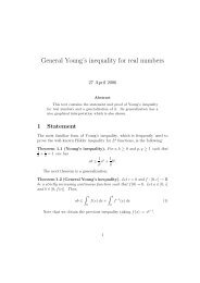
c 1<br />
c 1<br />
c 1 c 2<br />
c<br />
c 2<br />
c 1 #c 2<br />
2<br />
c 1 #c 2 c 1 #c 2<br />
Figure 3: The rum c 1#c 2 of two circles c 1, c 2 in the Poincaré disk, with signed<br />
radii r 1 = 1, +1, −1, r 2 = −0.25, +0.25, −0.25 and distance 0.5 between their<br />
centers<br />
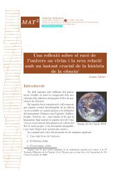
c 1 c 1<br />
c<br />
c 2<br />
2<br />
c 1 c 2<br />
c<br />
c 1 #c 1 #c 2<br />
2<br />
c 1 #c 2
<strong>HOROSPHERES</strong> <strong>IN</strong> <strong>HYPERBOLIC</strong> <strong>GEOMETRY</strong> 19<br />
Figure 4: The rum c 1#c 2 of two circles c 1, c 2 in the Poincaré disk, with signed<br />
radii r 1 = +1,+1, −1, r 2 = −1,+1, −1 and distance 3 between their centers<br />
Proposition 4.6. Let c 1 , c 2 be counter-clockwise oriented circles<br />
or points in H 2 . Then the rum c 1 #c 2 of c 1 and c 2 is a circle<br />
containing both c 1 and c 2 .<br />
Proof. c 1 , c 2 are counter-clockwise oriented. Hence their support<br />
maps θ 1 , θ 2 support convex-sided, and their planes do not intersect<br />
H 2 . Now θ ∗ lies below θ 1 and θ 2 with respect to each<br />
generator of C+ 2 (cf. Lemma 4.1). Therefore the plane of θ∗ does<br />
not intersect H 2 . Hence each θ ∗ supports c 1 #c 2 convex-sided<br />
and contains c 1 and c 2 .<br />
□<br />
Proposition 4.7. Let c 1 , c 2 be counter-clockwise oriented smooth<br />
regular boundaries of h-convex bodies K 1 , K 2 in H 2 . Then the<br />
rum c ∗ = c 1 #c 2 of c 1 and c 2 is the counter-clockwise oriented<br />
smooth regular boundary of an h-convex body K ∗ , also called rum<br />
K ∗ = K 1 #K 2 of K 1 and K 2 . Moreover K 1 , K 2 ⊂ K ∗ .<br />
Proof. The curves c 1 , c 2 are oriented counter-clockwise and h-<br />
convex, hence their θ 1 , θ 2 support convex-sided.<br />
The second order situation of c 1 and c 2 at related points determines<br />
the second order situation of c ∗ at the envelope point.<br />
For more details at this place, one should especially take into<br />
account:<br />
1) The support map of the osculating circle of a c in H 2 is given<br />
by the intersection of the osculating plane of θ in R 3 1 with C2 + .<br />
2) The intersection of the osculating plane of θ with C+ 2 is the<br />
osculating circle of the curve θ in R 3 1 (use the Meusnier formula).<br />
And<br />
3) The rum in C+ 2 of the osculating circles of θ 1 and θ 2 in C+ 2 is<br />
equal to the osculating circle of θ 1 #θ 2 (to this use 2) and (26) ).<br />
Now the second order situation of c 1 , c 2 is given by their osculating<br />
circles osc 1 , osc 2 in H 2 . Therefore the circle (cf. Proposition<br />
4.6) osc 1 #osc 2 describes the second order situation of c 1 #c 2 .<br />
Hence θ 1 #θ 2 supports c 1 #c 2 convex-sided, c 1 #c 2 is regular and
20 E. GALLEGO, A. REVENTÓS, G. SOLANES, AND E. TEUFEL<br />
oriented counter-clockwise. And osc 1 #osc 2 is the osculating circle<br />
of c 1 #c 2 . Therefore c 1 #c 2 is h-convex. Finally by Proposition<br />
4.6, K 1 , K 2 ⊂ K ∗ . □<br />
References<br />
[Fil70] Jay P. Fillmore, Barbier’s theorem in the Lobachevski plane, Proc.<br />
Amer. Math. Soc. 24 (1970), 705–709.<br />
[San67] L. A. Santaló, Horocycles and convex sets in hyperbolic plane, Arch.<br />
Math. (Basel) 18 (1967), 529–533.<br />
[San68] , Horospheres and convex bodies in hyperbolic space, Proc.<br />
Amer. Math. Soc. 19 (1968), 390–395.<br />
[San76] Luis A. Santaló, Integral geometry and geometric probability,<br />
Addison-Wesley Publishing Co., Reading, Mass.-London-<br />
Amsterdam, 1976, With a foreword by Mark Kac, Encyclopedia<br />
of Mathematics and its Applications, Vol. <strong>1.</strong><br />
Departament de Matemàtiques, Universitat Autònoma de Barcelona,<br />
08193–Bellaterra (Barcelona), Spain<br />
E-mail address: egallego@mat.uab.cat, agusti@mat.uab.cat, solanes@mat.uab.cat<br />
Fachbereich Mathematik, Universität Stuttgart, Pfaffenwaldring<br />
57, 70550 Stuttgart, Germany<br />
E-mail address: eteufel@mathematik.uni-stuttgart.de