NOISE EFFECTS IN THE QUANTUM SEARCH ALGORITHM FROM ...

Int. J. Appl. Math. Comput. Sci., 2012, Vol. 22, No. 2, 493–499
DOI: 10.2478/v10006-012-0037-2
NOISE EFFECTS IN THE QUANTUM SEARCH ALGORITHM FROM THE
VIEWPOINT OF COMPUTATIONAL COMPLEXITY
PIOTR GAWRON, JERZY KLAMKA, RYSZARD WINIARCZYK
Institute of Theoretical and Applied Informatics
Polish Academy of Sciences, ul. Bałtycka 5, 44-100 Gliwice, Poland
e-mail: gawron@iitis.pl
We analyse the resilience of the quantum search algorithm in the presence of quantum noise modelled as trace preserving
completely positive maps. We study the influence of noise on the computational complexity of the quantum search algorithm.
We show that it is only for small amounts of noise that the quantum search algorithm is still more efficient than any
classical algorithm.
Keywords: quantum algorithms, quantum noise, algorithm complexity.
1. Introduction
It is often said that the strength of quantum computation
lies in the phenomena of quantum superposition and quantum
entanglement. These features of quantum computation
allow performing the computation on all possible
inputs that fit the quantum register. One of the greatest
achievements in the theory of quantum algorithms is the
quantum search algorithm introduced by Grover. A detailed
description of this algorithm can be found in the
works of Grover (1996; 1997; 1998) and Bugajski (2001).
Any physical implementation of a quantum computer
will be error-prone because of the interaction of the computing
device with the environment. In this paper we investigate
the resilience of Grover’s algorithm in the presence
of quantum noise. We use the language of density
matrices and quantum channels. Our goal is to find the
maximal amount of noise for which the quantum algorithm
is better, in terms of the mean number of operations,
than the classical algorithm. We aim to achieve this objective
by considering some classes of quantum channels
modelling environmentally induced noise.
The paper is organised as follows. In Section 2 we
provide a short review of the subject. In Section 3 we
describe the formalism of quantum information theory. In
Section 4 we present the quantum search algorithm. In
Section 5 we introduce the noise model we have applied
to the system. In Section 6 we analyse the results, and
finally in Section 7 we present some conclusions.
2. Review of existing work
The problem of the influence of noise on the quantum
search algorithm has been extensively studied by various
researchers. Barnes and Warren (1999) discuss the
influence of the classical field upon a quantum system
implementing Grover’s algorithm. Pablo-Norman and
Ruiz-Altaba (1999) pose a question similar to ours, but
use a Gaussian noise model, which in their case is not
described in the language of quantum channels. Long
et al. (2000) analyse how imperfections in realizations of
quantum gates influence the probability of the success of
the quantum search algorithm. Konstadakis and Ellinas
(2001) analyse the behaviour of the quantum search algorithm
implemented with the use of noisy π/4 rotation
gates.
The effect of unitary noise on the quantum search algorithm
is studied by Shapira et al. (2003). Shenvi et al.
(2003) examine the robustness of Grover’s search algorithm
to a random phase error in the oracle and analyse
the complexity of the search process. Azuma (2005) studies
decoherence in Grover’s quantum search algorithm
using a perturbation method. Zhirov and Shepelyansky
(2006) use the methods of quantum trajectories to study
the effects of dissipative decoherence on the accuracy of
Grover’s quantum search algorithm. Salas (2008) numerically
simulates Grover’s algorithm introducing random
errors of two types: one- and two-qubit gate errors and
memory ones.

494 P. Gawron et al.
3. Formalism of quantum information
3.1. Dirac notation. Throughout this paper we use the
Dirac notation. The symbol |ψ〉 denotes a complex column
vector, 〈ψ| denotes the row vector dual to |ψ〉. The
scalar product of vectors |ψ〉, |φ〉 is denoted by 〈ψ|φ〉. The
outer product of these vectors is denoted by |φ〉〈ψ|. Vectors
are labelled in a natural way: |0〉 := ( 1 0 ), |1〉 := ( 0 1 ).
Notation such as |φψ〉 denotes the tensor product of vectors
and is equivalent to |φ〉⊗|ψ〉.
and the partial trace with respect to system A reads
tr A (ρ AB )= ∑ m
ρmμ
mν = ρB .
Given the state of the composed system ρ AB ,the
state of subsystems can by found by taking the partial
trace of ρ AB with respect to one of the subsystems. It
should be noted that tracing-out is not a reversible operation,
so, in a general case,
3.2. Density operators. The most general state of
a quantum system is described by a density operator. In
quantum mechanics a density operator ρ is defined as a
Hermitian (ρ = ρ † ) positive semi-definite (ρ ≥ 0) trace
one (tr(ρ) =1) operator. When a basis is fixed, the density
operator can be written in the form of a matrix. Diagonal
density matrices can be identified with probability
distributions, and therefore this formalism is a natural extension
of probability theory.
Density operators are usually called quantum states.
The set of quantum states is convex (Bengtsson and Życzkowski,
2006), and its boundary consists of pure states
which in matrix terms are rank one projectors. Convex
combinations of pure states lie inside the set and are called
mixed states.
3.2.1. Entanglement. Entanglement is one of the most
important phenomena in quantum information theory. We
say that a state ρ is separable iff it can be written in the
following form:
ρ =
M∑
q i ρ A i ⊗ ρ B i , (1)
i=1
where q i > 0 and ∑ M
i=1 q i =1. A state that is not separable
is called entangled. It is an open problem of great
importance and under investigation to decide if a given
quantum state is entangled or not.
3.2.2. Subsystems. Given two states ρ A , ρ B of two
systems A and B, the product state ρ AB of the composed
system is obtained by taking the Kronecker product of the
states, i.e., ρ AB = ρ A ⊗ ρ B .
Let [ρ AB ] kl be a matrix representing a quantum system
composed of two subsystems of dimensions M and
N. We want to index the matrix elements of ρ using
two double indices [ρ AB ]mμ, so that Latin indices correspond
to the system A and Greek indices correspond
nν
to the system B. The relation between the indices is
k =(m − 1)N + μ, l =(n − 1)N + ν. The partial
trace with respect to system B reads
tr B (ρ AB )= ∑ μ
ρmμ
nμ = ρA ,
ρ AB ≠tr A (ρ AB ) ⊗ tr B (ρ AB ). (2)
3.3. Completely Positive Trace-Preserving (CPTP)
maps. We say that an operation is physical if it transforms
density operators into density operators. Additionally,
we assume that physical operations are linear. Therefore,
in order for an operation Φ(·) to be physical, it has
to fulfil the following set of conditions:
(i) For any operator ρ its image under operation Φ has to
have its trace and positivity preserved, i.e., if tr(ρ) =
1,ρ ≥ 0,ρ = ρ † , then tr(Φ(ρ)) = 1, Φ(ρ) ≥
0, Φ(ρ) =Φ(ρ) † .
(ii) The operator Φ has to be linear:
( ) ∑
Φ p i ρ i = ∑ p i Φ(ρ i ) . (3)
i
i
(iii) The extension of the operator Φ to any larger dimension
that acts trivially on the extended system has
to preserve positivity. This feature is called complete
positivity. This means that for all positive semidefinite
ρ, ξ ≥ 0, the following holds:
(Φ ⊗ I dim (ξ) )(ρ ⊗ ξ) =Φ(ρ) ⊗ ξ ≥ 0. (4)
CPTP maps are often called quantum channels.
3.3.1. Kraus form. Any operator Φ that is completely
positive and trace preserving can be expressed in the socalled
Kraus form (Bengtsson and Życzkowski, 2006),
which consists of a finite set {E k } of Kraus operators,
i.e., matrices that fulfil the completeness relation:
∑
k E k † E k = I. The image of the state ρ under the map
Φ is given by
Φ(ρ) = ∑ k
E k ρE k † . (5)
3.4. Measurement. Quantum states cannot be observed
directly. In the literature, two main types of measurements
are considered: von Neumann measurements

Noise effects in the quantum search algorithm from the viewpoint of computational complexity
495
and POVM (Positive Operator Valued Measure) measurements.
In this paper we use only von Neumann measurements,
but for the sake of completeness we also define
POVM measurements.
The mathematical formulation of von Neumann measurement
is given by a map from a set of projection operators
to real numbers.
Let us consider an orthogonal complete set of projection
operators P = {P i } N i=1 and the set of real measurement
outcomes O = {o i } N i=1 . The mapping P → O
is called the von Neumann measurement. Assuming the
system is in the state ρ, the probability p i of measuring
outcome o i is given by the relation p i =tr(P i ρ).
The POVM measurement can be considered a generalisation
of the von Neumann measurement. Let us
take a set of positive operators F = {F i } N i=1 such that
∑ N
i=1 F i = I and the set of real measurement outcomes
O = {o i } N i=1 . The mapping F → O is called the POVM
measurement. Given the system in the state ρ, the probability
p i of measuring the outcome o i isgivenbytherelation
p i =tr(F i ρ).
4. Overview of Grover’s algorithm
Grover’s unordered database search algorithm is one of
the most important quantum algorithms. This is due to
the fact that many algorithmic problems can be reduced to
exhaustive search.
The main idea of the algorithm is to amplify the probability
of the state which represents the sought element.
The algorithm is probabilistic and may fail to return the
proper result. Fortunately, the probability of success is
reasonably high.
4.1. Problem. Let X be a set and let f : X →{0, 1},
such that
{ 1 if x = x0 ,
f(x) =
(6)
0 if x ≠ x 0 ,
x ∈ X, for some marked x 0 ∈ X.
For simplicity, we assume that X is a set of binary
strings of length n. Therefore, |X| = 2 n and
f : {0, 1} n →{0, 1}. We can map the set X to a set
of states over C ⊗2n in a natural way: x ↔|x〉, forming
an a orthogonal, complete set of vectors. The goal of the
algorithm is to find the marked element.
4.2. Algorithm. Grover’s algorithm is composed of
two main procedures: the oracle and diffusion.
With the use of elementary quantum gates the oracle
can be constructed using ancilla |q〉 in the following way:
O|x〉|q〉 = |x〉|q ⊕ f(x)〉, (7)
where ⊕ denotes addition modulo 2. If the register |q〉 is
prepared in the state
|q〉 = H|1〉 = |0〉−|1〉 √ , (8)
2
where H denotes the Hadamard gate, then, by substitution,
Eqn. (7) can be written as
O|x〉 |0〉−|1〉 √
2
By tracing out the ancilla, we obtain
=(−1) f(x) |x〉 |0〉−|1〉 √
2
. (9)
O|x〉 = −(−1) f(x) |x〉. (10)
4.2.2. Diffusion. The operator D rotates any state
around the state
|ψ〉 = √ 1
2∑
n −1
|x〉, (11)
2
n
where D can be written as
x=0
D = −H ⊗n (2|0〉〈0|−I)H ⊗n =2|ψ〉〈ψ|−I. (12)
4.2.3. Initialisation. We begin in the ground state
|0 ...00〉. In the first step of the algorithm we apply the
Hadamard gate H ⊗n to the entire register. This transforms
the initial state into flat superposition of computational
base states:
H ⊗n |0 ...0〉 = √ 1 (|0 ...00〉 + ···+ |1 ...11〉) .
n
(13)
4.2.4. Grover iteration. The core of the algorithm
consists of the applications of the so-called Grover iteration
gate G = D · O. This procedure causes the sought
state to be amplified and other states to be attenuated.
4.2.5. Number of iterations. The application of the
diffusion operator to the base state |x〉 gives
D|x〉 = −|x 0 〉 + 2 ∑
|y〉. (14)
N
The application of this operator on any state gives
y
4.2.1. Oracle. By an oracle we mean a function that
marks one defined element. In the case of Grover’s algorithm,
the marking of the element is done by the negation
of the amplitude of the sought state.
D|x〉 = ∑ α i (−|x〉 + 2 N y ∑ i
y
= ∑ (−α i +2s)|x〉,
i
|y〉)

496 P. Gawron et al.
where
s = 1 ∑
α i . (15)
N
A k-fold application of Grover’s iteration G to the
initial state |s〉 leads to (Bouwmeester et al., 2000; Bugajski,
2001)
G k |s〉 = α k
∑
x≠x 0
|x〉 + β k |x 0 〉, (16)
with real coefficients
1
α k = √ cos (2k +1)θ, β k =sin(2k +1)θ,
N − 1
(17)
where θ is an angle that fulfils the relation
sin(θ) = √ 1 . (18)
N
Therefore the coefficients α k ,β k are periodic functions of
k. After a series of iterations, β k rises. The influence of
the marked state |x 0 〉 on the state of the register results
in the evolution of the initial state |s〉 towards the marked
state.
β k attains its maximum after approximately π 4
√
N
steps. The number of steps needed to transfer the initial
state towards the marked state is of order O( √ N). Inthe
classical case the number of steps is of order O(N).
4.2.6. Measurement. The last step of Grover’s algorithm
is a von Neumann measurement. The probability of
obtaining the proper result is |β k | 2 .
5. Noise model
The above discussion of the quantum search algorithm has
been conducted using the state vector formalism. In order
to incorporate noise into the quantum computation model,
we have to make use of density operators which define the
quantum state in the most general way.
5.1. Quantum noise. Microscopic systems that are
governed by the laws of quantum mechanics are hard to
control and, at the same time, to separate from the environment.
The interaction with the environment introduces
noise into the quantum system. Therefore any future
quantum computer will also be prone to noise.
One-qubit noise. There are several one-parameter families
of one-qubit noisy channels that are typically discussed
in the literature (Nielsen and Chuang, 1999). We
present them briefly below.
Depolarising channel. This is a bi-stochastic channel that
transforms any state into a maximally mixed state with
i
a given probability α. The family of channels can be defined
using a four-element set of Kraus operators
{ √ √ √ √1 α α α − αI,
3 σ x,
3 σ y, z}
3 σ ,
where
[ ]
[ ]
1 0
0 1
I = , σ
0 1
x = ,
1 0
[ ]
[ ]
0 −i
1 0
σ y =
, σ
i 0
z =
0 −1
are Pauli matrices.
Amplitude damping. The amplitude damping channel
transforms |1〉 into |0〉 with a given probability α. The
state |0〉 remains unchanged. The set of Kraus operators
is {[ 1 0
0
√ 1 − α
]
,
[
0
√ α
0 0
]}
.
Phase damping. Phase damping in a quantum phenomenon
describes the loss of quantum information without
the loss of energy. It is described by the following set
of Kraus operators:
{[ ] [ ]}
1
√ 0 0 0
,
0 1 − α 0 √ .
α
Bit flip. The bit flip family of channels is the quantum
version of the classical binary symmetric channel. The
action of the channel might be interpreted in the following
way: it flips the state of a qubit from |0〉 to |1〉 and from |1〉
to |0〉 with probability α. Kraus operators for this family
of channels consist of a matrix proportional to the identity
and a matrix proportional to the negation gate,
{√ √ }
1 − αI, ασx .
Phase flip. The phase flip channel acts similarly to the bit
flip channel with the distinction that a σ z gate is applied
randomly to the qubit
{√ √ }
1 − αI, ασz .
Bit-phase flip. The bit-phase flip channel may be considered
a joint application of bit and phase flip gates to a
qubit. Its Kraus operators are as follows:
{√ √ }
1 − αI, ασy .
In all of the above families of channels, the real parameter
α ∈ [0, 1] can be interpreted as the amount of
noise introduced by the channel.

Noise effects in the quantum search algorithm from the viewpoint of computational complexity
497
|0〉
|0〉
.
|0〉
H ⊗n
Iterate √ N π 4 times
Diffusion
Oracle
|x〉→(−1) f(x) |x〉 H ⊗n |0〉→|0〉
|x〉→−|x〉 H ⊗n Noise
ρ t+1=Φ(ρ t)
forx>0
.
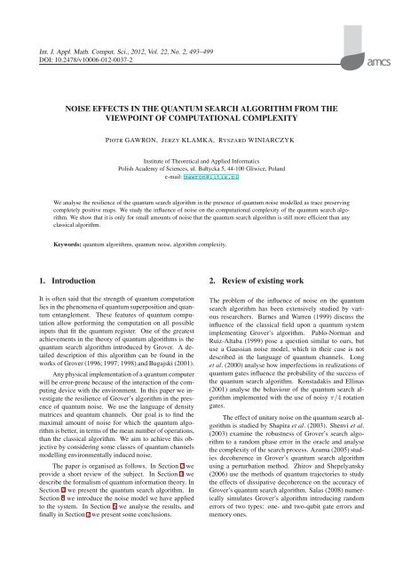
Fig. 1. Circuit for Grover’s algorithm extended with a non-unitary noisy channel.
Multiqubit local channels. Our goal is to extend the
noise acting on distinct qubits to the entire registers. We
assume that the appearance of an error on a given qubit is
independent of an error appearing on any other qubits.
In order to apply noise operators to multiple qubits,
we form a new set of Kraus operators acting on a larger
Hilbert space.
We assume that we have the set of n one-qubit Kraus
operators {e k } n k=1 . We construct the new set of nN operators
{E k } nN
k=1
that act on a Hilbert space of dimension
2 N by applying the following formula:
where
{E k } = ⋃ {e i1 ⊗ e i2 ⊗ ...⊗ e iN }, (19)
I
I = {i 1 } n i 1=1 ×{i 2 } n i 2=1 × ...×{i N } n i N =1.
One should note that the extended channel Φ(ρ) =
∑
k E kρE † k
is by definition local (Bengtsson and Życzkowski,
2006).
By applying Eqn. (19) to the sets of operators listed
above, we obtain one-parameter families of local noisy
channels, which we use in further investigations.
5.2. Application of noise to the algorithm. In order to
simulate noisy behaviour of the system implementing the
algorithm, we apply a noisy channel after every Grover
iteration. The evolution of the system is described by
the following procedure, which is graphically depicted in
Fig. 1:
1. Prepare the system in state ρ 0 := |0 ⊗n 〉〈0 ⊗n |.
2. ρ := H ⊗n ρ 0 H ⊗n†
3. ⌊ π 4
√
N⌋ times do:
(a) apply Grover’s iteration ρ := GρG † ,
(b) apply noise ρ := Φ(ρ).
4. Perform an orthogonal measurement in the computational
basis. The probability of finding the sought
element ξ is p = 〈ξ|ρ|ξ〉.
This approach simplifies the physical reality, but it is
sufficient to study the robustness of the algorithm in the
presence of noise. In order to study the discussed problem,
we make use of numerical simulations. Therefore
some simplification is necessary as the size of the problem
grows exponentially fast with the number of qubits.
The tool we use is quantum-octave (Gawron
et al., 2010), a library that contains functions for simulation
and analysis of quantum processes.
In our model we assume that it is easy to verify the
correctness of the quantum search algorithm. It is an
assumption usually made in the complexity analysis of
search algorithms.
6. Analysis of the influence of noise on the
efficiency of the algorithm
An interesting question arises: “What is the maximal
amount of noise for which Grover’s algorithm is more efficient
than any classical search algorithm”
Grover’s algorithm is probabilistic, therefore we cannot
expect to obtain a valid outcome with certainty. We
assume that if the algorithm fails in a given run we will
rerun it. There is a certain number of reruns for which the
quantum algorithm is worse than the classical. We are interested
only in the statistical behaviour of algorithm and
calculate the mean value of repetitions.
Let k = ⌊ N 2 / √ π
4 N⌋ be the maximal number of single
runs of Grover’s algorithm for which quantum search
is faster than the classical one.
We compute the minimal value of success probability
p min of a single run of Grover’s algorithm for which we
obtain a valid result with confidence C,
{
p min =min 1 − (1 − p) k ≥ C } . (20)
p
Numerically obtained values of p min for the confidence
level C =0.95 for Grover’s algorithm are listed in
Table 1.

498 P. Gawron et al.
Table 1. Values of k and p min for Grover’s algorithm.
Size of the system k p min
N =2 3 1 0.95000
N =2 4 2 0.77639
N =2 5 3 0.63160
N =2 6 5 0.45072
N =2 7 7 0.34816
N =2 8 10 0.25887
For our numerical experiment we assume that the
sought element ξ lies in the “middle” of the space of elements,
i.e., ξ =2 n−1 .
Plots in Fig. 2 depict the influence of the noise parameter
α on a successful run of Grover’s algorithm acting
on six qubits. These values of the parameter α for
which the plots are above the threshold level p min can be
considered the amounts of noise which do not make the
quantum search algorithm less efficient than the classical
search algorithms.
We can compare the probabilities from plots in Fig. 2
and these for other sizes of quantum registers with p min
and find the value of the noise parameter α for which it is
equal to p min . The results of the comparison are collected
in Table 2 for the confidence level C =0.95 and for the
channels described in Section 5.
Table 2. Maximal values of the noise parameter α for which
Grover’s search algorithm is as efficient as the classical
search algorithm in terms of the number of uses of the
oracle.
C =0.95 depolarising amplitude damping phase damping
N =2 4 0.025 0.069 0.177
N =2 5 0.032 0.010 0.204
N =2 6 0.031 0.104 0.190
N =2 7 0.026 0.094 0.158
N =2 8 0.020 0.075 0.122
bit flip phase flip bit-phase flip
N =2 4 0.025 0.047 0.018
N =2 5 0.032 0.054 0.024
N =2 6 0.031 0.050 0.023
N =2 7 0.026 0.041 0.020
N =2 8 0.020 0.031 0.015
In the case of three qubits we have found that, if we
expect a confidence level C =0.95 or higher, Grover’s
algorithm is never better than the classical search algorithm.
This means that if we want to get the result with
high probability, we have to repeat the quantum search so
many times that it is more efficient to perform this task
classically.
In other cases we have obtained the values of the
noise parameter α between ∼ 0.010 and ∼ 0.2 depending
on the noise type and the system size. We observe
that, even if the amount of noise is larger in bigger systems
(which causes the algorithm to be less efficient), the
noise is compensated by the quantum speed-up.
The results gathered in Table 2 do not form a monotonic
pattern. To understand this fact, we have to take into
account that two factors influence these numbers. The first
one is due to the fact that the same value of the noise parameter
α has greater influence on the quantum system
for bigger numbers of qubits and for larger N the number
of Grover iterations and noisy channel applications
k is increasing. At the same time, the more qubits used
to perform the search algorithm, the more important the
quantum speed-up.
7. Summary
In this work we have shown a new way of analysing the
influence of quantum noise on the quantum search algorithm.
Our method uses the model of density matrices and
quantum channels represented in the Kraus form.
We can conclude that the simulations and analysis
have shown that it is only for small amounts of noise that
the quantum search algorithm is still more efficient than
any classical algorithm.
From our numerical results we conclude that different
forms of noise have different impact on the efficiency
of the quantum search algorithm. The least destructive
form of noise is phase damping, more destructive is amplitude
damping, and the most destructive is the depolarizing
channel.
Further work would have to take into account quantum
error correcting codes and more precise noise models
dependent on the implementation. One of the research
directions would be to analyse the quantum search algorithm
in the framework of control Hamiltonians taking
into account Markovian approximation of quantum noise.
Acknowledgment
We acknowledge the financial support by the Polish Ministry
of Science and Higher Education (MNiSzW) under
the grants N N519 442339 and N N516 481840. The work
of Piotr Gawron was partially supported by the MNiSW
project IP2010 009770. The numerical calculations presented
in this work were performed on the Leming server
of the Institute of Theoretical and Applied Informatics,
Polish Academy of Sciences.
References
Azuma, H. (2005). Higher-order perturbation theory for
decoherence in Grover’s algorithm, Physical Review A
72(4): 42305.
Barnes, J.P. and Warren, W.S. (1999). Decoherence and
programmable quantum computation, Physical Review A
60(6): 4363–4374.

Noise effects in the quantum search algorithm from the viewpoint of computational complexity
499
Probability of success
1
0.8
0.6
0.4
0.2
depolarizing channel
amplitude damping channel
phase damping channel
p min for N =2 6 0
Probability of success
1
0.8
0.6
0.4
0.2
bit flip channel
phase flip channel
bit-phase flip channel
p min for N =2 6
0
0 0.05 0.1 0.15 0.2
noise level α
0 0.05 0.1 0.15 0.2
noise level α
Fig. 2. Probabilities of a successful run of Grover’s algorithm as a function of the noise parameter α: case of six qubits. The value for
which the plots attain the threshold p min is shown in Table 1.
Bengtsson, I. and Życzkowski, K. (2006). Geometry of Quantum
States. An Introduction to Quantum Entanglement, Cambridge
University Press, Cambridge.
Bouwmeester, D., Ekert, A. and Zeilinger, A. (2000). The
Physics of Quantum Information: Quantum Cryptography,
Quantum Teleportation, Quantum Computation, Physics
and Astronomy Online Library, Springer,
http://www.springer.com/physics/quantum
+physics/book/978-3-540-66778-0.
Bugajski, S. (2001). Quantum search, Archiwum Informatyki
Teoretycznej i Stosowanej 13(2): 143–150.
Gawron, P., Klamka, J., Miszczak, J.A. and Winiarczyk, R.
(2010). Extending scientific computing system with structural
quantum programming capabilities, Bulletin of the
Polish Academy of Sciences: Technical Sciences 58(1): 77–
88.
Grover, L. (1996). A fast quantum mechanical algorithm for
database search, Proceedings of the 28th Annual ACM
Symposium on the Theory of Computation, Philadelphia,
PA, USA, pp. 212–219.
Grover, L.K. (1997). Quantum mechanics helps in searching for
a needle in a haystack, Physical Review Letters 79(2): 325.
Grover, L.K. (1998). A framework for fast quantum mechanical
algorithms, Proceedings of the 30th Annual ACM Symposium
on Theory of Computing (STOC), Dallas, TX, USA,
pp. 53–62.
Konstadakis, C. and Ellinas, D. (2001). Noisy Grover’s Searching
Algorithm, OSA Technical Digest Series, Optical Society
of America, Rochester/New York, NY.
Long, G.L., Li, Y.S., Zhang, W.L. and Tu, C.C. (2000). Dominant
gate imperfection in Grover’s quantum search algorithm,
Physical Review A 61(4): 42305.
Nielsen, M. and Chuang, I. (1999). Quantum Computation and
Quantum Information, Cambridge University Press, Cambridge.
Pablo-Norman, B. and Ruiz-Altaba, M. (1999). Noise in
Grover’s quantum search algorithm, Physical Review A
61(1): 12301.
Salas, P.J. (2008). Noise effect on Grover algorithm, The European
Physical Journal D 46(2): 365–373.
Shapira, D., Mozes, S. and Biham, O. (2003). Effect of unitary
noise on Grover’s quantum search algorithm, Physical
Review A 67(4): 42301.
Shenvi, N., Brown, K.R. and Whaley, K.B. (2003). Effects
of a random noisy oracle on search algorithm complexity,
Physical Review A 68(5): 52313.
Zhirov, O.V. and Shepelyansky, D.L. (2006). Dissipative decoherence
in the Grover algorithm, The European Physical
Journal D 38(2): 405–408.
Piotr Gawron, Ph.D., Eng., works in the Quantum
Systems of Informatics Group of the Institute
of Theoretical and Applied Informatics,
Polish Academy of Sciences. His main areas
of research include noise in quantum processes,
quantum games, and simulation of quantum processes.
Jerzy Klamka, Ph.D., Prof., is a full member
of the Polish Academy of Sciences and works
in the Quantum Systems of Informatics Group
of the Institute of Theoretical and Applied Informatics,
Polish Academy of Sciences. The main
areas of his research include controllability and
observability of linear and non-linear dynamical
systems, as well as mathematical foundations of
quantum computations. He is the author of numerous
monographs and many papers published
in international journals.
Ryszard Winiarczyk, Ph.D., Eng., received the
M.Sc and Ph.D. degrees from the Silesian University
of Technology in Gliwice. In 2001, he
was appointed the head of the Quantum System
of Informatics Group in the Institute of Theoretical
and Applied Informatics, Polish Academy
of Sciences. His main research interest in the
quantum informatics domain is the development
of software environment for quantum computations.
Received: 3 March 2011
Revised: 10 August 2011