NOISE EFFECTS IN THE QUANTUM SEARCH ALGORITHM FROM ...
NOISE EFFECTS IN THE QUANTUM SEARCH ALGORITHM FROM ...
NOISE EFFECTS IN THE QUANTUM SEARCH ALGORITHM FROM ...

Create successful ePaper yourself
Turn your PDF publications into a flip-book with our unique Google optimized e-Paper software.
Noise effects in the quantum search algorithm from the viewpoint of computational complexity<br />
497<br />
|0〉<br />
|0〉<br />
.<br />
|0〉<br />
H ⊗n<br />
Iterate √ N π 4 times<br />
<br />
<br />
<br />
<br />
<br />
<br />
<br />
<br />
<br />
Diffusion<br />
<br />
Oracle<br />
|x〉→(−1) f(x) |x〉 H ⊗n |0〉→|0〉<br />
|x〉→−|x〉 H ⊗n Noise<br />
<br />
ρ t+1=Φ(ρ t) <br />
<br />
forx>0<br />
<br />
<br />
<br />
<br />
<br />
<br />
<br />
<br />
<br />
<br />
<br />
<br />
.<br />
<br />
<br />
Fig. 1. Circuit for Grover’s algorithm extended with a non-unitary noisy channel.<br />
Multiqubit local channels. Our goal is to extend the<br />
noise acting on distinct qubits to the entire registers. We<br />
assume that the appearance of an error on a given qubit is<br />
independent of an error appearing on any other qubits.<br />
In order to apply noise operators to multiple qubits,<br />
we form a new set of Kraus operators acting on a larger<br />
Hilbert space.<br />
We assume that we have the set of n one-qubit Kraus<br />
operators {e k } n k=1 . We construct the new set of nN operators<br />
{E k } nN<br />
k=1<br />
that act on a Hilbert space of dimension<br />
2 N by applying the following formula:<br />
where<br />
{E k } = ⋃ {e i1 ⊗ e i2 ⊗ ...⊗ e iN }, (19)<br />
I<br />
I = {i 1 } n i 1=1 ×{i 2 } n i 2=1 × ...×{i N } n i N =1.<br />
One should note that the extended channel Φ(ρ) =<br />
∑<br />
k E kρE † k<br />
is by definition local (Bengtsson and Życzkowski,<br />
2006).<br />
By applying Eqn. (19) to the sets of operators listed<br />
above, we obtain one-parameter families of local noisy<br />
channels, which we use in further investigations.<br />
5.2. Application of noise to the algorithm. In order to<br />
simulate noisy behaviour of the system implementing the<br />
algorithm, we apply a noisy channel after every Grover<br />
iteration. The evolution of the system is described by<br />
the following procedure, which is graphically depicted in<br />
Fig. 1:<br />
1. Prepare the system in state ρ 0 := |0 ⊗n 〉〈0 ⊗n |.<br />
2. ρ := H ⊗n ρ 0 H ⊗n†<br />
3. ⌊ π 4<br />
√<br />
N⌋ times do:<br />
(a) apply Grover’s iteration ρ := GρG † ,<br />
(b) apply noise ρ := Φ(ρ).<br />
4. Perform an orthogonal measurement in the computational<br />
basis. The probability of finding the sought<br />
element ξ is p = 〈ξ|ρ|ξ〉.<br />
This approach simplifies the physical reality, but it is<br />
sufficient to study the robustness of the algorithm in the<br />
presence of noise. In order to study the discussed problem,<br />
we make use of numerical simulations. Therefore<br />
some simplification is necessary as the size of the problem<br />
grows exponentially fast with the number of qubits.<br />
The tool we use is quantum-octave (Gawron<br />
et al., 2010), a library that contains functions for simulation<br />
and analysis of quantum processes.<br />
In our model we assume that it is easy to verify the<br />
correctness of the quantum search algorithm. It is an<br />
assumption usually made in the complexity analysis of<br />
search algorithms.<br />
6. Analysis of the influence of noise on the<br />
efficiency of the algorithm<br />
An interesting question arises: “What is the maximal<br />
amount of noise for which Grover’s algorithm is more efficient<br />
than any classical search algorithm”<br />
Grover’s algorithm is probabilistic, therefore we cannot<br />
expect to obtain a valid outcome with certainty. We<br />
assume that if the algorithm fails in a given run we will<br />
rerun it. There is a certain number of reruns for which the<br />
quantum algorithm is worse than the classical. We are interested<br />
only in the statistical behaviour of algorithm and<br />
calculate the mean value of repetitions.<br />
Let k = ⌊ N 2 / √ π<br />
4 N⌋ be the maximal number of single<br />
runs of Grover’s algorithm for which quantum search<br />
is faster than the classical one.<br />
We compute the minimal value of success probability<br />
p min of a single run of Grover’s algorithm for which we<br />
obtain a valid result with confidence C,<br />
{<br />
p min =min 1 − (1 − p) k ≥ C } . (20)<br />
p<br />
Numerically obtained values of p min for the confidence<br />
level C =0.95 for Grover’s algorithm are listed in<br />
Table 1.