A robust controller design method and stability analysis of an ...
A robust controller design method and stability analysis of an ...
A robust controller design method and stability analysis of an ...

Create successful ePaper yourself
Turn your PDF publications into a flip-book with our unique Google optimized e-Paper software.
Int. J. Appl. Math. Comput. Sci., 2006, Vol. 16, No. 3, 345–356<br />
A ROBUST CONTROLLER DESIGN METHOD AND STABILITY ANALYSIS<br />
OF AN UNDERACTUATED UNDERWATER VEHICLE<br />
CHENG SIONG CHIN, MICHEAL WAI SHING LAU<br />
EICHER LOW, GERALD GIM LEE SEET<br />
Robotic Research Centre, Department <strong>of</strong> Mech<strong>an</strong>ical <strong><strong>an</strong>d</strong> Aerospace Engineering<br />
N<strong>an</strong>y<strong>an</strong>g Technological University, Singapore 639798<br />
e-mail: mcschin1@yahoo.com<br />
The problem <strong>of</strong> <strong>design</strong>ing a stabilizing feedback <strong>controller</strong> for <strong>an</strong> underactuated system is a challenging one since a nonlinear<br />
system is not stabilizable by a smooth static state feedback law. A necessary condition for the asymptotical stabilization <strong>of</strong> <strong>an</strong><br />
underactuated vehicle to a single equilibrium is that its gravitational field has nonzero elements corresponding to unactuated<br />
dynamics. However, global asymptotical <strong>stability</strong> (GAS) c<strong>an</strong>not be guar<strong>an</strong>teed. In this paper, a <strong>robust</strong> proportional-integralderivative<br />
(PID) <strong>controller</strong> on actuated dynamics is proposed <strong><strong>an</strong>d</strong> unactuated dynamics are shown to be global exponentially<br />
bounded by the Sørdalen lemma. This gives a necessary <strong><strong>an</strong>d</strong> sufficient condition to guar<strong>an</strong>tee the global asymptotic <strong>stability</strong><br />
(GAS) <strong>of</strong> the URV system. The proposed <strong>method</strong> is first adopted on a remotely-operated vehicle RRC ROV II <strong>design</strong>ed<br />
by the Robotic Research Centre in the N<strong>an</strong>y<strong>an</strong>g Technological University (NTU). Through the simulation using the ROV<br />
Design <strong><strong>an</strong>d</strong> Analysis toolbox (RDA) written at the NTU in the MATLAB/SIMULINK environment, the RRC ROV II is<br />
<strong>robust</strong> against parameter perturbations.<br />
Keywords: underwater vehicle, underactuated, stabilizable, <strong>robust</strong> <strong>controller</strong>, simulation<br />
1. Introduction<br />
In this paper, a nonlinear system consisting <strong>of</strong> actuated<br />
<strong><strong>an</strong>d</strong> unactuated dynamics is studied. The problem <strong>of</strong> <strong>design</strong>ing<br />
a stabilizing feedback <strong>controller</strong> for underactuated<br />
systems is a challenging one since the system is not stabilizable<br />
by a smooth static state feedback law (Brockett,<br />
1983). Fossen (1994) <strong><strong>an</strong>d</strong> Yuh (1990) showed that a fully<br />
actuated vehicle (a vehicle where the control <strong><strong>an</strong>d</strong> configuration<br />
vector have the same dimension) c<strong>an</strong> be asymptotically<br />
stabilized in position <strong><strong>an</strong>d</strong> velocity by a smooth<br />
feedback law. Byrnes et al. (1991) explained why underactuated<br />
vehicles having zero gravitational field are not<br />
asymptotically stabilizable to a single equilibrium. On the<br />
other h<strong><strong>an</strong>d</strong>, Wichlund et al. (1995) stated that the vehicle<br />
with gravitational <strong><strong>an</strong>d</strong> restoring terms in unactuated dynamics<br />
is stabilizable to a single equilibrium point. However,<br />
it is a necessary but not sufficient condition to state<br />
that the vehicle is asymptotically stabilizable. The closedloop<br />
asymptotical <strong>stability</strong> <strong>of</strong> the vehicle in the earth-fixed<br />
frame needs to be examined further.<br />
A different <strong>method</strong> th<strong>an</strong> those proposed in (Wichlund<br />
et al., 1995) is used to show that actuated dynamics<br />
in the earth-fixed frame is exponentially decaying under<br />
the nonlinear <strong>controller</strong>. The <strong>method</strong> described in (Wichlund<br />
et al., 1995) uses a nonlinear dynamic control law to<br />
achieve a neat closed loop actuated subsystem that yields<br />
<strong>an</strong> exponentially decaying solution, but gives low flexibility<br />
in <strong>design</strong>ing the control law since nonlinear vehicle<br />
dynamics have to be known exactly for nonlinear dynamic<br />
c<strong>an</strong>cellation.<br />
In this paper, a <strong>robust</strong> Proportional-Integral-<br />
Derivative (PID) <strong>controller</strong> is chosen due to its simplicity<br />
in implementation <strong><strong>an</strong>d</strong> its common use in industry. PID is<br />
<strong>design</strong>ed only for actuated dynamics, such that it provides<br />
a necessary <strong><strong>an</strong>d</strong> sufficient condition for the asymptotic <strong>stability</strong><br />
<strong>of</strong> unactuated dynamics. In this <strong>method</strong>, unactuated<br />
dynamics are self-stabilizable <strong><strong>an</strong>d</strong> converge exponentially<br />
to zero. With the <strong>controller</strong>, the actuated dynamics become<br />
asymptotically stable while the actuated states in the<br />
unactuated dynamic equation diminish. Applying the asymptotic<br />
<strong>stability</strong> lemma by Sørdalen (Søodalen <strong><strong>an</strong>d</strong> Egel<strong><strong>an</strong>d</strong><br />
1993; 1995; Sørdalen et al., 1993) to the unactuated<br />
dynamic equation provides a validation for the initial argument<br />
<strong>of</strong> convergence to zero. Thus the vehicle in the<br />
earth-fixed frame, which is self-stabilizable in unactuated<br />
dynamics, is asymptotically stable.<br />
The paper is org<strong>an</strong>ized as follows: A nonlinear<br />
model <strong>of</strong> <strong>an</strong> underactuated ROV, developed by the Robotic<br />
Research Centre in the N<strong>an</strong>y<strong>an</strong>g Technological University<br />
(Koh et al., 2002b; Micheal et al., 2003), is presented<br />
in Section 2. Section 3 describes a necessary con-
346<br />
C.S. Chin et al.<br />
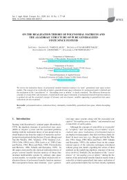
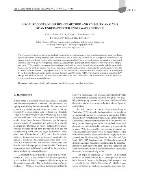
Front view <strong>of</strong> the RRC ROV II<br />
Side view <strong>of</strong> the RRC ROV II<br />
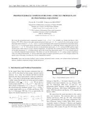
Fig. 1. Thruster configuration on the ROV platform.<br />
dition for a vehicle with gravitational <strong><strong>an</strong>d</strong> restoring terms<br />
in unactuated dynamics to be stabilizable. In Sections 4<br />
<strong><strong>an</strong>d</strong> 5, a <strong>robust</strong> PID <strong>controller</strong> is proposed for the asymptotic<br />
<strong>stability</strong> <strong>of</strong> the vehicle in the earth-fixed frame<br />
which is self-stabilizable in unactuated dynamics. The results<br />
<strong>of</strong> computer simulations using the ROV Design <strong><strong>an</strong>d</strong><br />
Analysis (RDA) toolbox written at the NTU in the MAT-<br />
LAB/SIMULINK environment are presented in Section 6.<br />
2. Nonlinear Model <strong>of</strong> the Underactuated<br />
ROV<br />
The dynamic behavior <strong>of</strong> <strong>an</strong> underwater vehicle is <strong>design</strong>ed<br />
through Newton’s laws <strong>of</strong> linear <strong><strong>an</strong>d</strong> <strong>an</strong>gular momentum.<br />
The equations <strong>of</strong> motion <strong>of</strong> such vehicles are<br />
highly nonlinear (Fossen, 1994) <strong><strong>an</strong>d</strong> coupled due to hydrodynamic<br />
forces which act on the vehicle. Usually, the<br />
ROV model c<strong>an</strong> be described in either a body-fixed or <strong>an</strong><br />
earth-fixed frame.<br />
2.1. Body-Fixed Model <strong>of</strong> the Underactuated ROV.<br />
It is convenient to write the general dynamic <strong><strong>an</strong>d</strong> kinematic<br />
equations for the ROV in the body-fixed frame:<br />
M v ˙v + C v (v)v + D v (v)v + g(η) =B v u v , (1)<br />
˙η = J(η)v, (2)<br />
where B v ∈ R 6×4 is a thruster configuration matrix (defined<br />
by the thruster layout as shown in Fig. 1), u v ∈ R 4<br />
is <strong>an</strong> input vector, v =[u, v, w, p, q, r] T ∈ R 6 is a velocity<br />
vector, η =[x, y, z, φ, θ, ψ] T ∈ R 3 × S 3 is a position<br />
<strong><strong>an</strong>d</strong> orientation vector, M v ∈ R 6×6 is a mass inertia<br />
matrix with added mass coefficients, C v (v) ∈ R 6×6 is<br />
a centripetal <strong><strong>an</strong>d</strong> Coriolis matrix with added mass coefficients,<br />
D v (v) ∈ R 6×6 is a diagonal hydrodynamic damping<br />
matrix, <strong><strong>an</strong>d</strong> g(η) ∈ R 6 is a vector <strong>of</strong> buoy<strong>an</strong>cy <strong><strong>an</strong>d</strong><br />
gravitational forces <strong><strong>an</strong>d</strong> moments. The ROV path relative<br />
to the earth-fixed reference frame is given by the kinematic<br />
equation (2), where J(η) = J(η 2 ) ∈ R 6×6 <strong><strong>an</strong>d</strong><br />
η 2 =[φ, θ, ψ] T is <strong>an</strong> Euler tr<strong>an</strong>sformation matrix.<br />
2.2. An Earth-Fixed Model <strong>of</strong> the Underactuated<br />
ROV. Sometimes, we need to express the ROV model<br />
from the body coordinate to earth-fixed coordinates (Fossen,<br />
1994) by performing the coordinate tr<strong>an</strong>sformation<br />
(η, v) ↦→ μ<br />
(η, ˙η) defined by<br />
[ ] [ ][ ]<br />
η I 0 η<br />
=<br />
, (3)<br />
˙η 0 J(η) v<br />
where the tr<strong>an</strong>sformation matrix, J, has the following<br />
form:<br />
⎡<br />
c(ψ)c(θ) −s(ψ)c(φ)+c(ψ)s(θ)s(φ)<br />
s(ψ)c(θ) c(ψ)c(θ)+s(φ)s(θ)s(ψ)<br />
J(η) =<br />
−s(θ)<br />
c(θ)s(φ)<br />
0 0<br />
⎢<br />
⎣ 0 0<br />
0 0
A <strong>robust</strong> <strong>controller</strong> <strong>design</strong> <strong>method</strong> <strong><strong>an</strong>d</strong> <strong>stability</strong> <strong><strong>an</strong>alysis</strong> <strong>of</strong> <strong>an</strong> underactuated underwater vehicle<br />
347<br />
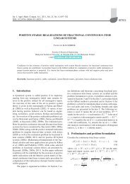
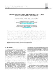
Fig. 2. Experimental RRC ROV II in a swimming pool.<br />
⎤<br />
s(ψ)s(φ)+c(ψ)c(φ)s(θ) 0 0 0<br />
−c(ψ)s(φ)+s(θ)s(ψ)c(φ) 0 0 0<br />
c(θ)c(φ) 0 0 0<br />
0 1 s(φ)t(θ) c(φ)t(θ)<br />
,<br />
⎥<br />
0 0 c(φ) −s(φ) ⎦<br />
0 0 s(φ)/c(θ) c(φ)/c(θ)<br />
(4)<br />
where c(·) =cos(·), t(·) =t<strong>an</strong>(·) <strong><strong>an</strong>d</strong> s(·) =sin(·). The<br />
coordinate tr<strong>an</strong>sformation μ is a global diffeomorphism<br />
which is <strong>an</strong>alogous to a similarity tr<strong>an</strong>sformation in linear<br />
systems. This tr<strong>an</strong>sformation is undefined for θ = ±90 o .<br />
To overcome this singularity, a quaternion approach must<br />
be considered. However, in our study this problem does<br />
not exist because the vehicle is not sufficient to operate at<br />
θ = ±90 o . Moreover, the vehicle is completely stable in<br />
roll <strong><strong>an</strong>d</strong> pitch, <strong><strong>an</strong>d</strong> the thruster actuation is not sufficient to<br />
move the vehicle to operate at this <strong>an</strong>gle. The ROV model<br />
in earth-fixed coordinates becomes<br />
M η (˙η, η)¨η + C η (˙η,η)˙η<br />
+ D η (˙η, η)˙η + g η (η) =B η u η , (5)<br />
where M η (˙η,η) =J −T M v J −1 , C η (˙η, η) =J −T (C −<br />
M v J −1 J)J ˙ −1 , D η (˙η, η) = J −T D v J −1 ,g η (η) =<br />
J −T g v <strong><strong>an</strong>d</strong> B η u η = J −T B v u v .<br />
3. Stabilizability<br />
In this section a <strong>method</strong> to test system stabilizability is<br />
presented. In general, the vector g ( η) c<strong>an</strong> be further decomposed<br />
into elements corresponding to actuated dynamics<br />
(the first to third <strong><strong>an</strong>d</strong> sixth elements), g a (η), <strong><strong>an</strong>d</strong><br />
the element corresponding to unactuated dynamics (the<br />
fourth <strong><strong>an</strong>d</strong> fifth elements), g u (η). The pro<strong>of</strong> <strong>of</strong> Theorem 3<br />
in (Wichlund et al., 1995) regards the system given by<br />
Eqns. (1) <strong><strong>an</strong>d</strong> (2). Suppose that (η, v) =(0, 0) is <strong>an</strong> equilibrium<br />
point <strong>of</strong> the system. If g u (η) is zero, then there<br />
exists no continuous <strong><strong>an</strong>d</strong> discontinuous state feedback law<br />
(Byrnes <strong><strong>an</strong>d</strong> Isidori, 1991), k(η, v) :R 6 ⇒ R 4 , which<br />
makes (0, 0) <strong>an</strong> asymptotically stable equilibrium.<br />
However, the RRC ROV II <strong>of</strong> Fig. 2 has a<br />
gravitational field at unactuated dynamics, g u (η) =<br />
[29.61 cos θ sin φ 29.61 sin θ] T ≠0but no gravitational<br />
field at g a (η) =0. Therefore, the RRC ROV II may be<br />
stabilizable at the equilibrium point. However, it is a necessary,<br />
but not sufficient, condition to state that the ROV<br />
is asymptotically stabilizable at the equilibrium point. Inevitably,<br />
it gives rise to the need <strong>of</strong> finding a control law<br />
to stabilize the ROV at the equilibrium point.<br />
4. Asymptotic Stabilization <strong>of</strong> Actuated<br />
Dynamics by Smooth State Feedback<br />
In Sections 4 <strong><strong>an</strong>d</strong> 5, the concepts in the asymptotic stabilization<br />
<strong>of</strong> actuated dynamics are as follows: (i) by observation,<br />
the unactuated dynamics in (7) are self-stabilizable<br />
<strong><strong>an</strong>d</strong> exponentially decaying; (ii) use a <strong>robust</strong> PID <strong>controller</strong><br />
to globally asymptotically stabilize the actuated dynamics<br />
in (6); (iii) with actuated dynamics, globally asymptotically<br />
stable (GAS) f 1 implies that the actuated dynamics<br />
h 2 in the unactuated equation (7) becomes zero;<br />
(iv) finally, step (i) is verified by the Sørdalen lemma. For<br />
clarity, this section is divided into two parts. The problem<br />
definition is given in Part I, perturbation on the ROV’s parameters<br />
<strong><strong>an</strong>d</strong> the <strong>controller</strong> <strong>design</strong> <strong><strong>an</strong>d</strong> the <strong>stability</strong> <strong><strong>an</strong>alysis</strong><br />
on actuated dynamics are provided in Part II.<br />
4.1. Problem Definition. The separation <strong>of</strong> the entire<br />
system into actuated <strong><strong>an</strong>d</strong> unactuated subsystems, as de-
348<br />
scribed in (Micheal et al., 2003), yields<br />
¨η a = f 1 (˙η a ,η a ,t)+h 1 (˙η u ,η u ,t)+B ηa u a , (6)<br />
¨η u = f 2 (˙η u ,η u ,t)+h 2 (˙η a ,η a ,t)+B ηu u u , (7)<br />
where<br />
1<br />
f 1 (˙η a ,η a ,t)=−<br />
det(M η ) M η 22<br />
× [ C η11 (v, η)+D η11 (v, η) ] ˙η a ,<br />
1<br />
h 1 (˙η u ,η u ,t)=−<br />
det(M η ) M η 12<br />
g ηu<br />
+ M η12 C η21 (v, η)˙η u ,<br />
1<br />
f 2 (˙η u ,η u ,t)=−<br />
det(M η ) M η 11<br />
× [ C η22 (v, η)+D η22 (v, η) ] ˙η u ,<br />
1<br />
h 2 (˙η a ,η a ,t)=−<br />
det(M η ) M η 11<br />
g ηu<br />
− M η12 C η12 (v, η)˙η a ,<br />
det(M η )=M η22 M η11 − M η12 2 ,<br />
η =[zxyψ| φθ] T =[η a | η u ], η a ∈ R 3 × S, η u ∈ R 2 ,<br />
B η =[B ηa B ηu ] are the input matrices for the actuated<br />
<strong><strong>an</strong>d</strong> unactuated dynamics in (5). Note that the subscripts<br />
‘a’ <strong><strong>an</strong>d</strong> ‘u’ refer to the actuated <strong><strong>an</strong>d</strong> unactuated dynamics,<br />
respectively.<br />
Let η d denote the desired set points (position <strong><strong>an</strong>d</strong> orientation)<br />
in the earth-fixed frame. The error <strong>of</strong> this actuated<br />
position about the hovering or station-keeping condition<br />
c<strong>an</strong> be written down as<br />
e = η a − η d ⇒ ė =˙η a , ë =¨η a . (8)<br />
Substituting the preceding equation into (6) <strong><strong>an</strong>d</strong> (7) yields<br />
ë = f 1 (ė, e, t)+h 1 (˙η u ,η u ,t)+B ηa u a , (9)<br />
¨η u = f 2 (˙η u ,η u ,t)+h 2 (ė, e, t)+B ηu u u . (10)<br />
Consider h 1 (˙η u ,η u ,t) as a perturbation to (9) <strong><strong>an</strong>d</strong> assume<br />
that it could converge (or exponentially decay) to zero as<br />
time increases. Then (9) becomes<br />
ë = f 1 (ė, e, t)+B ηa u a . (11)<br />
The qu<strong>an</strong>tity h 1 (˙η u ,η u ,t) decays in (9) as the restoring<br />
forces (based on the ROV <strong>design</strong> intention) in the<br />
η u = {φ, θ} directions enable these two motions to stabilize<br />
themselves effectively instead <strong>of</strong> destabilizing the<br />
C.S. Chin et al.<br />
system. Furthermore, if η a c<strong>an</strong> be proven to be asymptotically<br />
stable, i.e., e → 0 as t → 0, the term h 2 (ė, e, t)<br />
in (10) decays <strong><strong>an</strong>d</strong> becomes<br />
¨η u = f 2 (˙η u ,η u ,t)+B ηu u u . (12)<br />
Applying the asymptotic <strong>stability</strong> pro<strong>of</strong> for η u validates<br />
the initial assumption <strong>of</strong> h 1 (˙η u ,η u ,t) → 0 as t →∞.<br />
The following will illustrate the above-mentioned <strong>method</strong>.<br />
Assuming that the perturbation h 1 (˙η u ,η u ,t) is<br />
bounded by a decaying exponential ∫ function <strong><strong>an</strong>d</strong> u a =<br />
u PID = −Bη −1<br />
τ<br />
a<br />
(K p e + K i 0 e dt + K d de<br />
dt<br />
) for the actuated<br />
subsystem exists, (9) becomes ë = f 1 (ė, e, t) +<br />
B ηa u PID . The asymptotical <strong>stability</strong> <strong>of</strong> η a , i.e., e → 0 as<br />
t → 0 is proven in the following.<br />
4.2. Perturbation on the ROV’s Parameters. To test<br />
the <strong>robust</strong>ness <strong>of</strong> PID control schemes, the ROV’s mass<br />
inertia, centripetal <strong><strong>an</strong>d</strong> Coriolis matrix <strong><strong>an</strong>d</strong> the diagonal<br />
hydrodynamic damping matrix are allowed to vary within<br />
the limits specified in (14) <strong><strong>an</strong>d</strong> (16). These variations c<strong>an</strong><br />
be attributed to the inaccuracy in modeling <strong><strong>an</strong>d</strong> possible<br />
ch<strong>an</strong>ges in the mass distribution in the ROV. The limits<br />
were obtained using a computer-aided <strong>design</strong> (CAD)<br />
s<strong>of</strong>tware, Pro-E. By ch<strong>an</strong>ging the mass properties <strong>of</strong> each<br />
thruster, pod <strong><strong>an</strong>d</strong> stainless-steel frame as shown in Fig. 2,<br />
a different mass inertia matrix was obtained. By evaluating<br />
the differences between the nominal <strong><strong>an</strong>d</strong> new mass<br />
inertia matrices, the following limits c<strong>an</strong> be determined:<br />
The bounds m η1 <strong><strong>an</strong>d</strong> m η1 are obtained by first evaluating<br />
the inverse <strong>of</strong> the body-fixed mass inertia matrix,<br />
M −1<br />
v<br />
in (5) obtained from the CAD s<strong>of</strong>tware, Pro-E:<br />
M η (˙η,η) =J −T M v J −1 ,<br />
M η (˙η,η) −1 = JM −1<br />
v J T . (13)<br />
Substituting Mv −1 that r<strong>an</strong>ges from −0.001 to 0.01 at J =<br />
I (as the Euler <strong>an</strong>gles are small) in (4) results in m η1 =<br />
−0.001 <strong><strong>an</strong>d</strong> m η1 =0.01. Hence, the bounds on Mη −1<br />
1<br />
become<br />
where<br />
m η1 I ≤ M −1<br />
η 1<br />
≤ m η1 I, (14)<br />
Mη −1 [<br />
2<br />
1<br />
= M η22 Mη22 M η11 − M ] −1<br />
η12 . (15)<br />
The upper bounds on the centripetal <strong><strong>an</strong>d</strong> Coriolis matrix<br />
<strong><strong>an</strong>d</strong> the diagonal hydrodynamic damping matrix in<br />
C η1 are set as<br />
C η1 ≤ K A ‖L‖ + K B , (16)<br />
where K A > 0(=0.001) <strong><strong>an</strong>d</strong> K B > 0(=0.001) are<br />
const<strong>an</strong>t <strong><strong>an</strong>d</strong> obtained indirectly from the CAD s<strong>of</strong>tware,<br />
Pro-E,<br />
C η1 = [ C η11 (v, η)+D η11 (v, η) ] , (17)<br />
‖·‖being the Euclide<strong>an</strong> norm <strong><strong>an</strong>d</strong> L =[e ė] T .
A <strong>robust</strong> <strong>controller</strong> <strong>design</strong> <strong>method</strong> <strong><strong>an</strong>d</strong> <strong>stability</strong> <strong><strong>an</strong>alysis</strong> <strong>of</strong> <strong>an</strong> underactuated underwater vehicle<br />
349<br />
4.3. Controller Design <strong><strong>an</strong>d</strong> Stability Analysis <strong>of</strong> the<br />
Actuated Dynamic. Implementing the control law<br />
into (11) yields<br />
ë = Mη −1<br />
1<br />
C η1 ė<br />
[ ∫ τ<br />
− Mη −1<br />
de<br />
]<br />
1<br />
K p e + K i e dt + K d . (18)<br />
0 dt<br />
State-space equations become<br />
x 1 =<br />
∫ τ<br />
0<br />
e T dt, ẋ 1 = e T ,<br />
x 2 = e T , ẋ 2 =ė T ,<br />
x 3 =ė T ,<br />
ẋ 3 =ë T<br />
= M −1<br />
η 1<br />
C η1 x 3 − M −1 K d x 3 − Mη −1<br />
1<br />
K p x 2<br />
η 1<br />
− M −1<br />
η 1<br />
K i x 1 , (19)<br />
where the superscript T in e T indicates the tr<strong>an</strong>spose <strong>of</strong> e.<br />
Equation (19) in the matrix form becomes<br />
⎡ ⎤<br />
⎢<br />
⎣<br />
ẋ 1<br />
ẋ 2<br />
ẋ 3<br />
⎥<br />
⎦<br />
A<br />
{ ⎡<br />
}} ⎤{<br />
⎡ ⎤<br />
0 I n 0<br />
x 1<br />
⎢<br />
⎥ ⎢ ⎥<br />
= ⎣ 0 0 I n ⎦ ⎣x 2 ⎦.<br />
−Mη −1<br />
1<br />
K i −Mη −1<br />
1<br />
K p −Mη −1<br />
1<br />
(K d + C η1 ) x 3<br />
(20)<br />
To <strong>an</strong>alyze the system’s <strong>robust</strong> <strong>stability</strong>, consider the<br />
following Lyapunov function:<br />
V (x) =x T Px<br />
= 1 ∫ t<br />
T [α 2 e(τ)dτ + α 1 e +ė]<br />
Mη1<br />
2<br />
0<br />
∫ t<br />
]<br />
×<br />
[α 2 e(τ)dτ +α 1 e+ė +ϖ T P 1 ϖ, (21)<br />
0<br />
where<br />
⎡ ∫ t ⎤<br />
⎢<br />
e(τ)dτ<br />
⎥<br />
ϖ = ⎣ 0 ⎦ ,<br />
e<br />
⎡<br />
⎤<br />
P 1 = 1 ⎣ α 2K p + α 1 K i α 2 K d + K i<br />
⎦ .<br />
2 α 2 K d + K i α 1 K d + K p<br />
(22)<br />
Hence<br />
P = 1 2<br />
⎡<br />
⎤<br />
α 2K p+α 1K i+α 2 2M η1 α 2K d +K i+α 1α 2M η1 α 2M η1<br />
× ⎢<br />
⎣α 2K d +K i+α 1α 2M η1 α 1K d +K p+α 2 1M η1 α 1M η1<br />
⎥<br />
⎦ .<br />
α 2M η1 α 1M η1 M η1<br />
(23)<br />
Since M η1 is a positive definite matrix, P is positive definite<br />
if, <strong><strong>an</strong>d</strong> only if, P 1 is positive definite. Now choose<br />
K p = k p I, K d = k d I <strong><strong>an</strong>d</strong> K i = k i I such that P in (23),<br />
i.e.,<br />
⎡<br />
α 2 k d + k i α 1 k d + k p<br />
⎣ α 2k p + α 1 k i α 2 k d + k i<br />
⎤<br />
⎦ (24)<br />
becomes positive definite. The following lemma gives the<br />
conditions for V (x) to become positive definite, bounded<br />
from above <strong><strong>an</strong>d</strong> below.<br />
Lemma 1. Assume that the following inequalities hold:<br />
α 1 > 0, α 2 > 0, α 1 + α 2 < 1,<br />
s 1 = α 2 (k p − k d ) − (1 − α 1 )k i<br />
− α 2 (1+α 1 −α 2 )m η1 > 0, (25)<br />
s 2 = k p +(α 1 −α 2 )k d − k i<br />
− α 1 (1+α 2 −α 1 )m η1 > 0. (26)<br />
Then P is positive definite <strong><strong>an</strong>d</strong> satisfies the following inequality<br />
(Rayleigh-Ritz) :<br />
λ(P )‖x‖ 2 ≤ V (x) ≤ λ(P )‖x‖ 2 , (27)<br />
in which<br />
{ 1 − α1 − α 2<br />
λ(P )=min<br />
2<br />
{ 1+α1 + α 2<br />
λ(P )=max<br />
2<br />
<strong><strong>an</strong>d</strong><br />
m η1 , s 1<br />
2 , s }<br />
2<br />
, (28)<br />
2<br />
m η1 , s 3<br />
2 , s 4<br />
2<br />
s 3 = α 2 (k p + k d )+(1+α 1 )k i<br />
}<br />
, (29)<br />
+(1+α 1 + α 2 )α 2 m η1 , (30)<br />
s 4 = α 1 m η1 (1 + α 1 + α 2 )<br />
+(α 1 + α 2 )k d + k p + k i . (31)
350<br />
Since P is positive definite,<br />
˙V (x) =x T (A T P + PA+ ˙ P )x<br />
− x T Qx<br />
⎡ ⎤<br />
+ 1 α 2 I<br />
⎢ ⎥<br />
2 xT ⎣α 1 I ⎦ Ṁη 1<br />
[α 2 I α 1 I I] x<br />
I<br />
+ 1 2 xT ⎡<br />
⎢<br />
⎣<br />
⎡<br />
⎢<br />
× ⎣<br />
Owing to Ṁη 1<br />
=0, (32) yields<br />
<strong><strong>an</strong>d</strong><br />
0 α 2 2 I α 1α 2 I<br />
α 2 2 I 2α 1α 2 I (α 2 1 + α 2)I<br />
α 1 α 2 I (α 2 1 + α 2)I α 1 I<br />
⎤<br />
⎥<br />
⎦<br />
⎤<br />
M η1 0 0<br />
⎥<br />
0 M η1 0 ⎦ x. (32)<br />
0 0 M η1<br />
˙V (x) ≤−γ‖x‖ 2 + ζ 2 m η1 ‖x‖ 2 (33)<br />
γ =min { α 2 k i ,α 1 k p − α 2 k d − k i ,k d<br />
}<br />
. (34)<br />
Let ‖L‖ ≤‖x‖. Denote by λ 2 = λ(R 2 ) the largest<br />
eigenvalue <strong>of</strong> R 2 ,<br />
⎡<br />
0 α 2 2<br />
⎢<br />
I α ⎤<br />
1α 2 I<br />
R 2 = ⎣ α 2 2I 2α 1 α 2 I (α 2 ⎥<br />
1 + α 2 )I ⎦ . (35)<br />
α 1 α 2 I (α 2 1 + α 2)I α 1 I<br />
As a result, the error system <strong>of</strong> the RRC ROV II, (20),<br />
is rendered GAS, if λ 2 is chosen small enough <strong><strong>an</strong>d</strong> the<br />
control gains K p ,K d <strong><strong>an</strong>d</strong> K i are large enough. The next<br />
step is to show that unactuated dynamics are exponentially<br />
bounded.<br />
5. Exponential Stability <strong>of</strong> Unactuated<br />
Dynamics Using Sørdalen’s Lemma<br />
As was shown in Section 4, the term h 2 (ė, e, t) consists<br />
<strong>of</strong> ė <strong><strong>an</strong>d</strong> e converged exponentially to zero, i.e., ė, e → 0<br />
as t → 0, yielding ¨η u = f 2 (˙η u ,η u ,t)+B ηu u u . The<br />
solution <strong>of</strong> the tracking error, e, c<strong>an</strong> be approximated as<br />
e = C e e −γet ⇒ ė = Cėe−γėt <strong><strong>an</strong>d</strong>, by substituting it into<br />
h 2 (ė, e, t), yields<br />
M η12 C η12<br />
h 2 (ė, e, t) =−<br />
M η22 M η11 − Mη 2 C e e −γet + M η11 g ηu<br />
12<br />
+ M η11 B η2 u u → 0 (36)<br />
C.S. Chin et al.<br />
for u u = −Bη −1<br />
2<br />
g ηu . The initial assumption h 1 (˙η u ,η u ,t)<br />
→ 0 as t →∞c<strong>an</strong> be validated by checking the asymptotic<br />
<strong>stability</strong> <strong>of</strong> η u . First, decompose η u into two part as<br />
follows:<br />
¨η u =<br />
[ ¨φ<br />
¨θ<br />
] [<br />
=<br />
f ˙φ( ˙φ, φ, t)+d ˙φ(t)<br />
f ˙θ( ˙θ, θ, t)+d ˙θ(t)<br />
]<br />
, (37)<br />
where d ˙φ(t),d˙θ(t) are considered as perturbations on ˙φ<br />
<strong><strong>an</strong>d</strong> ˙θ, respectively. The pro<strong>of</strong> <strong>of</strong> the exponential bound<br />
<strong>of</strong> the unactuated subsystems c<strong>an</strong> be obtained as shown<br />
below. The definite integral <strong>of</strong> f ˙φ( ˙φ, φ, t) from the time 0<br />
to t becomes<br />
∫ t<br />
∫ ∣ f ˙φ( ˙φ, t<br />
∣ φ, τ)dτ<br />
∣ ≤ ∣ f ∂ψ<br />
˙φI1<br />
0<br />
0 ∂τ /k ∣∣∣ a1∣ + ∂φ<br />
f ˙φI2<br />
∂τ /k a1∣<br />
+<br />
∣ f ∂θ<br />
˙φI3<br />
∂τ /k a1∣ +|f | dτ, (38)<br />
˙φI4<br />
where k a1 f ˙φI1<br />
,f ˙φI2<br />
,f ˙φI3<br />
,f ˙φI4<br />
c<strong>an</strong> be found in Appendix.<br />
Substituting I xx , I xy ,I xz ,I yz , ˙ψ, ˙φ <strong><strong>an</strong>d</strong> ˙θ into the<br />
preceding equation gives<br />
∫ t<br />
∫ ∣ f ˙φ( ˙φ, t<br />
φ, τ)dτ<br />
∣ ≤ |β 1 ˙θ|+|β2 ˙ψ|+|β 3 ˙φ| dτ<br />
∣<br />
∫ t<br />
0<br />
0<br />
≤<br />
0<br />
∫ t<br />
0<br />
β 1 |C ˙θe −α ˙θ τ |+β 2 |C ˙ψ e −α ˙ψ τ |<br />
+β 3 |C ˙φe −α ˙φ τ |+β 4 dτ,<br />
f ˙φ( ˙φ, φ, τ)+ɛ ˙φ<br />
dτ<br />
∣ ≤ β C ˙θ C ˙ψ C ˙φ<br />
1 +β 2 +β 3 , (39)<br />
α ˙θ<br />
α ˙ψ<br />
α ˙φ<br />
where β 1 , β 2 , β 3 , β 4 > 0. In the RRC ROV II, β 1 =<br />
15603, β 2 = 15470, β 3 =2.7, β 4 = 1650. Then d ˙φ(t)<br />
in (37) becomes<br />
|d ˙φ(t)| = |fż1 ż + fẋ1 ẋ + fẏ1 ẏ + f ˙ψ 1<br />
˙ψ + f ˙θ1<br />
˙θ|<br />
Define<br />
≤|fż1 ż| + |fẋ1 ẋ| + |fẏ1 ẏ|<br />
+ |f ˙ψ 1<br />
˙ψ| + |f ˙θ1<br />
˙θ|. (40)<br />
γ ˙φ<br />
=min { αż + αẋ,αż + αẏ,αẋ + αẏ,α ˙ ψ + α ˙θ,α˙ψ<br />
+ α ˙φ,α˙θ + α ˙φ,αż,αẋ,αẏ,α˙ψ ,α˙φ,α˙θ } (41)<br />
<strong><strong>an</strong>d</strong> ż = Cże−γż , ẋ = Cẋe−γẋ , ẏ = Cẏe−γẏ , ˙ψ =<br />
C ˙ψ e −γ ˙ψ , ∀αż,αẋ,αẏ,α˙ψ , where Cż,Cẋ,Cẏ,C ˙ψ > 0<br />
(Kreyszig, 1998) for <strong>an</strong> exponentially stable system.<br />
Then<br />
|d ˙φ(t)| ≤De −γ ˙φ t . (42)
A <strong>robust</strong> <strong>controller</strong> <strong>design</strong> <strong>method</strong> <strong><strong>an</strong>d</strong> <strong>stability</strong> <strong><strong>an</strong>alysis</strong> <strong>of</strong> <strong>an</strong> underactuated underwater vehicle<br />
351<br />
The solution <strong>of</strong> ¨φ(t) becomes<br />
| ˙φ(t)| =<br />
∣ e−[f ˙φ ( ˙φ,φ,t)+ɛ ˙φ]t ˙φ(0)<br />
∫ t<br />
+ e −[f ˙φ ( ˙φ,φ,t)+ɛ ˙φ]τ d ˙φ(τ)dτ<br />
0<br />
∣<br />
∫<br />
≤ e −P ˙φ t | ˙φ(0)| t<br />
+<br />
∣ e −P ˙φ τ d ˙φ(τ)dτ<br />
∣<br />
≤ e −P ˙φ t | ˙φ(0)| + |D[e−(P ˙φ +γ ˙φ )t − 1]|<br />
, (43)<br />
|P ˙φ<br />
+ γ ˙φ|<br />
where P ˙φ<br />
= ∫ t<br />
0 [f ˙φ( ˙φ, φ, τ) +ɛ ˙φ]dτ. Thus ˙φ(t) is<br />
bounded for <strong>an</strong>y t ≥ 0. Also, ˙φ(t) → 0 since<br />
1/|P ˙φ<br />
+ γ ˙φ|<br />
is small.<br />
Next, to show that φ(t) is bounded, consider<br />
∫ t<br />
|φ(t)| =<br />
∣<br />
˙φ(t)dτ + φ(0)<br />
∣<br />
Using (43), we get<br />
|φ(t)|≤<br />
∫ t<br />
0<br />
≤<br />
0<br />
∫ t<br />
0<br />
e −P ˙φ τ dτ| ˙φ(0)|<br />
D<br />
+<br />
|P ˙φ+γ ˙φ|<br />
≤− e−P ˙φ τ +1<br />
P ˙φ<br />
0<br />
| ˙φ(t)| dτ + |φ(0)|. (44)<br />
∫ t<br />
0<br />
(e −(P ˙φ +γ ˙φ )τ − 1) dτ +|φ(0)|<br />
| ˙φ(0)|− D<br />
e−(P<br />
˙φ +γ ˙φ )t<br />
|P ˙φ+γ 2 ˙φ|<br />
D<br />
− (t − 1) + |φ(0)|. (45)<br />
|P ˙φ<br />
+ γ ˙φ|<br />
Thus, φ(t) is bounded for all t ≥ 0 as 1/|P ˙φ<br />
+ γ ˙φ|<br />
is<br />
small for the RRC ROV II.<br />
Repeat the same procedure from (38) to (45) for<br />
f ˙θ( ˙θ, θ, τ). Substituting I xx ,I xy ,I xz ,I yz , see (Koh et al.,<br />
2002a), ˙ψ, ˙φ <strong><strong>an</strong>d</strong> ˙θ into the preceding equation gives the<br />
definite integral <strong>of</strong> f ˙φ(x, t),<br />
∫ t<br />
∣∫ ∣ f ˙θ( ˙θ, ∣∣∣ t<br />
θ, τ)dτ<br />
∣ = f ˙θ1<br />
dτ<br />
∣<br />
0<br />
≤<br />
≤<br />
0<br />
∫ t<br />
0<br />
∫ t<br />
0<br />
|α 1 ˙θ|+|α2 ˙ψ|+|α 3 ˙φ|+|α4 | dτ<br />
α 1 C<br />
˙θe −α ˙θ τ<br />
+ α 2 C ˙ψ e −α ˙ψ τ + α 3 C<br />
˙φe −α ˙φ τ<br />
+ α 4 dτ, (46)<br />
∣<br />
∫ t<br />
0<br />
∣<br />
[<br />
f ˙θ( ˙θ,<br />
] ∣∣∣<br />
θ, τ)+ɛ ˙θ dτ<br />
≤ α 1<br />
C ˙θ<br />
α ˙θ<br />
+ α 2<br />
C ˙ψ<br />
α ˙ψ<br />
C ˙φ<br />
+ α 4 , (47)<br />
α ˙φ<br />
where α 1 ,α 2 ,α 3 ,α 4 > 0. In RRC ROV II, α 1 =25.8,<br />
α 2 = 12270.8, α 3 = 12529, α 4 = 260378. Then d ˙θ(t)<br />
in (37) becomes<br />
|d ˙θ(t)| = |fż2 ż + fẋ2 ẋ + fẏ2 ẏ + f ˙ψ 2<br />
˙ψ + f ˙φ2<br />
˙φ|<br />
γ ˙θ<br />
≤|fż2 ż|+|fẋ2 ẋ|+|fẏ2 ẏ|+|f ˙ψ 2<br />
˙ψ|+|f ˙φ2<br />
˙φ|. (48)<br />
Define<br />
= min { αż + αẋ,αż + αẏ,αẋ + αẏ,α˙ψ + α ˙θ,<br />
α ψ ˙<br />
+ α ˙φ,α˙θ + α ˙φ,αż,αẋ,αẏ,<br />
α ψ ˙<br />
,α˙φ,α˙θ } , (49)<br />
<strong><strong>an</strong>d</strong> ż = Cże−γż , ẋ = Cẋe−γẋ , ẏ = Cẏe−γẏ , ˙ψ =<br />
C ˙ψ e −γ ˙ψ , ∀αż,αẋ,αẏ,α˙ψ , where Cż,Cẋ,Cẏ,C ˙ψ > 0<br />
(Kreyszig, 1998) for <strong>an</strong> exponentially stable system.<br />
Then<br />
|d ˙θ(t)| ≤De −γ ˙θ t . (50)<br />
The solution <strong>of</strong> ¨θ(t) becomes<br />
| ˙θ(t)| =<br />
∣ e−[f ˙θ ( ˙θ,θ,t)+ɛ ˙θ]t ˙θ(0)<br />
∫ t<br />
+ e −[f ˙θ ( ˙θ,θ,t)+ɛ ˙θ]τ d ˙θ(τ)dτ<br />
0<br />
∣<br />
∫<br />
≤ e −P ˙θ t | ˙θ(0)| t<br />
+<br />
∣ e −P ˙θ τ d ˙θ(τ)dτ<br />
∣<br />
0<br />
≤ e −P ˙θ t | ˙θ(0)| + |D[e(P ˙φ +γ ˙φ )t − 1]|<br />
, (51)<br />
|P ˙φ<br />
+ γ ˙φ|<br />
where P ˙θ<br />
= ∫ t<br />
0 [f ˙θ( ˙θ, θ, τ)+ɛ ˙θ]dτ. Thus ˙θ(t) is bounded<br />
for <strong>an</strong>y t ≥ 0. Also, ˙θ(t) → 0 as 1/|P ˙θ<br />
+ γ ˙θ|<br />
is small.<br />
Next, to show that θ(t) is bounded, consider<br />
|θ(t)| =<br />
∣<br />
≤<br />
∫ t<br />
0<br />
∫ t<br />
0<br />
˙θ(t)dτ + θ(0)<br />
∣<br />
| ˙θ(t)| dτ + |θ(0)|. (52)
352<br />
C.S. Chin et al.<br />
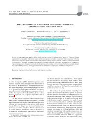
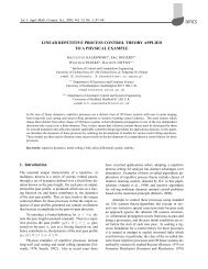
Fig. 3. SIMULINK library browser showing the RDA package.<br />
Using (51), we have<br />
1<br />
|θ(t)| ≤<br />
|P ˙θ<br />
+ γ ˙θ|<br />
+<br />
∫ t<br />
0<br />
∫ t<br />
+<br />
0<br />
∫ t<br />
0<br />
e −(P ˙θ +γ ˙θ )τ dτ<br />
e −P ˙θ τ dτ| ˙θ(0)|<br />
1<br />
dτ + |θ(0)| + |θ(0)|<br />
|P ˙θ<br />
+ γ ˙θ|<br />
≤− e−P ˙θ τ +1<br />
|<br />
P ˙θ(0)|−<br />
˙θ<br />
D<br />
e−(P<br />
˙θ +γ ˙θ )t<br />
|P ˙θ<br />
+ γ<br />
2 ˙θ|<br />
D<br />
− (t − 1) + |θ(0)|. (53)<br />
|P ˙θ<br />
+ γ ˙θ|<br />
Thus, θ(t) is bounded for <strong>an</strong>y t ≥ 0 as 1/|P ˙θ<br />
+ γ ˙θ|<br />
is<br />
small for the RRC ROV II.<br />
6. Computer Simulation Results<br />
This section illustrates the perform<strong>an</strong>ce <strong>of</strong> the proposed<br />
control scheme (in the presence <strong>of</strong> parameter perturbations)<br />
using the ROV Design <strong><strong>an</strong>d</strong> Analysis (RDA) package<br />
(see Fig. 3) developed at the NTU. The platform adopted<br />
for the development <strong>of</strong> RDA is MATLAB/SIMULINK.<br />
RDA provides the necessary resources for a rapid <strong><strong>an</strong>d</strong> systematic<br />
implementation <strong>of</strong> mathematical models <strong>of</strong> ROV<br />
systems with the focus on ROV modeling, control system<br />
<strong>design</strong> <strong><strong>an</strong>d</strong> <strong><strong>an</strong>alysis</strong>. The package provides examples<br />
ready for simulation. As is shown in Fig. 4, the block diagram<br />
<strong>of</strong> the proposed <strong>robust</strong> PID control was <strong>design</strong>ed.<br />
The perform<strong>an</strong>ce <strong>of</strong> the proposed control scheme was<br />
investigated in computer simulations using a Pentium IV,<br />
2.4 GHz computer. The simulation time was set to 100 s.<br />
The RRC ROV II parameters used in simulations c<strong>an</strong> be<br />
found in (Koh et al., 2002b). As the vehicle is currently<br />
equipped only with limited sensors, the desired position<br />
comm<strong><strong>an</strong>d</strong> values, v =[0.5 01000] T , are chosen with<br />
this purpose in mind. The objective is to regulate the position<br />
<strong>of</strong> the RRC ROV II to x =0.5 m <strong><strong>an</strong>d</strong> z =1mor<br />
the error signal equal to zero.<br />
The PID was selected due to its simplicity in implementation<br />
<strong><strong>an</strong>d</strong> its wide use in control applications. The<br />
control algorithm requires reduced computing resources,<br />
<strong><strong>an</strong>d</strong> is therefore suited for <strong>an</strong> on-board implementation.<br />
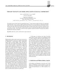
The PID control parameters were obtained from the Response<br />
Optimization (using the gradient descent <strong>method</strong>)<br />
toolbox in SIMULINK. The PID parameters are as follows:<br />
K p = diag{11, 11, 9, 1}, K i = diag{2, 4, 1, 2}<br />
<strong><strong>an</strong>d</strong> K d =diag{1, 1, 2, 1}. For example, the optimization
A <strong>robust</strong> <strong>controller</strong> <strong>design</strong> <strong>method</strong> <strong><strong>an</strong>d</strong> <strong>stability</strong> <strong><strong>an</strong>alysis</strong> <strong>of</strong> <strong>an</strong> underactuated underwater vehicle<br />
353<br />
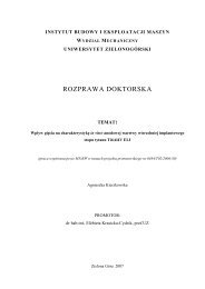
Fig. 4. SIMULINK block diagram <strong>of</strong> the proposed <strong>robust</strong> PID control.<br />
setting for the response in the x-direction was constrained<br />
as shown in Fig 7.<br />
As was already mentioned, the system is separated<br />
into actuated <strong><strong>an</strong>d</strong> unactuated states. In SIMULINK, it is<br />
modeled as a selector that ch<strong>an</strong>nels the actuated <strong><strong>an</strong>d</strong> unactuated<br />
states into two paths. The PID is used only for the<br />
actuated states while the unactuated ones are left uncontrolled,<br />
since then are self-stabilizable. The “<strong>robust</strong>” PID<br />
<strong>controller</strong> is called this way due to the perturbation <strong>of</strong> the<br />
mass inertia term as in (14). The perturbation <strong>of</strong> the mass<br />
inertia term r<strong>an</strong>ges from the minimum to the maximum <strong>of</strong><br />
≤ 0.01). This c<strong>an</strong> be modeled<br />
as a two-dimensional (2D) look-up table as shown<br />
in Fig. 4. During simulations, only the maximum value<br />
(or a worst-case perturbation) is used. Similarly, the perturbation<br />
for the centripetal, Coriolis <strong><strong>an</strong>d</strong> hydrodynamic<br />
damping matrix was set at (C η1 ≤ 0.001‖L‖ +0.001).<br />
Figure 5 shows simulation results for the <strong>robust</strong> PID<br />
control <strong>design</strong> with <strong><strong>an</strong>d</strong> without perturbations. It shows<br />
the position <strong>of</strong> the ROV with respect to the inertia frame.<br />
As c<strong>an</strong> be observed, the ROV control system is able to regulate<br />
about the selected reference position. The roll <strong><strong>an</strong>d</strong><br />
pitch motions are self-stabilizable about the zero position<br />
(as seen in Sørdalen’s pro<strong>of</strong>). From Fig. 5 it c<strong>an</strong> be seen<br />
that actuated states exhibit asymptotically stable phenomena,<br />
as proved by the Lyapunov <strong>stability</strong> theory. Notice<br />
that, in spite <strong>of</strong> parameter uncertainty, the ROV converges<br />
asymptotically to the desired position.<br />
the scale (−0.001 ≤ M −1<br />
η 1<br />
The flow chart shown in Fig. 6 illustrates the <strong>robust</strong><br />
PID <strong>design</strong> flow <strong><strong>an</strong>d</strong> <strong>method</strong>ology using RDA for the<br />
RRC ROV II. PID parameters are tuned <strong>of</strong>f-line by the<br />
Response Optimization toolbox using gradient descent till<br />
the desired responses are obtained. Besides, the tuning <strong>of</strong><br />
PID parameters c<strong>an</strong> be performed iteratively.<br />
7. Conclusion<br />
Besides using the ROV’s body-fixed coordinates in <strong>stability</strong><br />
<strong><strong>an</strong>alysis</strong>, the earth-fixed coordinate model was <strong>an</strong>alyzed.<br />
The stabilizability condition <strong>of</strong> the underactuated<br />
ROV was shown. The nonlinear system was separated<br />
into actuated <strong><strong>an</strong>d</strong> unactuated dynamic equations, <strong><strong>an</strong>d</strong> the<br />
asymptotical <strong>stability</strong> <strong>of</strong> closed-loop actuated equations,<br />
using the <strong>robust</strong> PID <strong>controller</strong> in the earth-fixed frame,<br />
was examined. This is based on the argument that the actuated<br />
dynamic equation could converge exponentially to<br />
zero by the PID <strong>controller</strong>. The asymptotic <strong>stability</strong> pro<strong>of</strong><br />
by Sørdalen in the unactuated dynamic equation provides<br />
a validation for the initial argument <strong>of</strong> the roll <strong><strong>an</strong>d</strong> pitch<br />
dynamics convergence to zero. The vehicle in the earthfixed<br />
frame with self-stabilizable unactuated dynamics is<br />
globally asymptotically stable with the <strong>robust</strong> PID <strong>controller</strong><br />
in actuated dynamics. This gives a necessary <strong><strong>an</strong>d</strong><br />
sufficient condition for the GAS <strong>of</strong> the ROV in the earthfixed<br />
frame.
354<br />
C.S. Chin et al.<br />
Fig. 5. Position response <strong>of</strong> the proposed <strong>robust</strong> PID control for x =0.5 m <strong><strong>an</strong>d</strong> z =1m.<br />
By simulating closed-loop control system <strong>design</strong> using<br />
the RDA package, the asymptotical <strong>stability</strong> <strong>of</strong> the <strong>robust</strong><br />
PID <strong>controller</strong> for the RRC ROV II c<strong>an</strong> be observed<br />
as position responses converge asymptotically to the desired<br />
position. The PID is said to be <strong>robust</strong> as the ROV’s<br />
mass inertia, centripetal <strong><strong>an</strong>d</strong> Coriolis matrix <strong><strong>an</strong>d</strong> the diagonal<br />
hydrodynamic damping matrix were allowed to vary<br />
within the limits obtained explicitly from the CAD s<strong>of</strong>tware,<br />
Pro-E.<br />
In summary, the RDA provides a systematic <strong>method</strong>ology<br />
in control system simulation <strong><strong>an</strong>d</strong> <strong>stability</strong> <strong><strong>an</strong>alysis</strong><br />
before implementation. It also provides necessary resources<br />
for a rapid implementation <strong>of</strong> mathematical models<br />
<strong>of</strong> ROV systems. The proposed control algorithm<br />
is quite simple <strong><strong>an</strong>d</strong> requires little computing resources,<br />
<strong><strong>an</strong>d</strong> is therefore suited for <strong>an</strong> on-board implementation.<br />
Simulation results show the effectiveness <strong>of</strong> the proposed<br />
<strong>method</strong>ology. If the real-time tuning <strong>of</strong> PID parameters<br />
is used, the control system could be more <strong>robust</strong> against<br />
larger parameters perturbation. As is shown in this paper,<br />
PID parameters c<strong>an</strong> be conveniently tuned by the<br />
Response Optimization toolbox in MATLAB/SIMULINK<br />
instead <strong>of</strong> the trial-<strong><strong>an</strong>d</strong>-error <strong>method</strong> <strong>of</strong> tuning.<br />
Acknowledgments<br />
The authors would like to th<strong>an</strong>k <strong><strong>an</strong>d</strong> acknowledge the contributions<br />
by all project team members from the NTU Robotics<br />
Research Centre, especially Mr. Lim Eng Cheng,<br />
Ms. Agnes S.K. T<strong>an</strong>, Ms. Ng Kwai Yee <strong><strong>an</strong>d</strong> Mr. You Kim<br />
S<strong>an</strong>.<br />
References<br />
Brockett R.W. (1983): Asymptotic <strong>stability</strong> <strong><strong>an</strong>d</strong> feedback stabilization,<br />
In: Differential Geometric Control Theory<br />
(R.W. Brockett, R.S. Millm<strong>an</strong> <strong><strong>an</strong>d</strong> H.J. Sussm<strong>an</strong>n, Eds.).<br />
— Boston: Birkhäuser, pp. 181–191.<br />
Byrnes C. <strong><strong>an</strong>d</strong> Isidori A. (1991): On the attitude stabilization <strong>of</strong><br />
rigid spacecraft. — Automatica, Vol. 27, No. 1, pp. 87–95.<br />
Fossen T.I. (1994): Guid<strong>an</strong>ce <strong><strong>an</strong>d</strong> Control <strong>of</strong> Oce<strong>an</strong> Vehicles.—<br />
New York: Wiley.<br />
Koh T.H., Lau M.W.S., Low E., Seet G.G.L. <strong><strong>an</strong>d</strong> Cheng P.L.<br />
(2002a): Preliminary studies <strong>of</strong> the modeling <strong><strong>an</strong>d</strong> control<br />
<strong>of</strong> a twin-barrel underactuated underwater robotic vehicle.<br />
— Proc. 7-th Int. Conf. Control, Automation, Robotics Vision,<br />
Singapore, pp. 1043–1047.
A <strong>robust</strong> <strong>controller</strong> <strong>design</strong> <strong>method</strong> <strong><strong>an</strong>d</strong> <strong>stability</strong> <strong><strong>an</strong>alysis</strong> <strong>of</strong> <strong>an</strong> underactuated underwater vehicle<br />
355<br />
Fig. 6. Flow chart <strong>of</strong> the <strong>robust</strong> PID <strong>design</strong> flow <strong><strong>an</strong>d</strong> <strong>method</strong>ology using RDA on the RRC ROV II.<br />
Koh T.H., Lau M.W.S., Low E., Seet G., Swei S. <strong><strong>an</strong>d</strong> Cheng<br />
P.L. (2002b): Development <strong><strong>an</strong>d</strong> improvement <strong>of</strong> <strong>an</strong> underactuated<br />
remotely operated vehicle (ROV) . — Proc.<br />
MTS/IEEE Int. Conf. Oce<strong>an</strong>s, Biloxi, MS, pp. 2039–2044.<br />
Kreyszig E. (1998): Adv<strong>an</strong>ced Engineering Mathematics. —<br />
New York: Wiley.<br />
Lau M.W.S., Swei S.S.M., Seet S.S.M., Low E. <strong><strong>an</strong>d</strong> Cheng P.L.<br />
(2003): Control <strong>of</strong> <strong>an</strong> underactuated remotely operated underwater<br />
vehicle. — Proc. Inst. Mech. Eng., Part 1: J. Syst.<br />
Contr., Vol. 217, No. 1, pp. 343–358.<br />
Søodalen O.J. <strong><strong>an</strong>d</strong> Egel<strong><strong>an</strong>d</strong> O. (1993): Exponential stabilization<br />
<strong>of</strong> chained nonholonomic systems. — Proc. 2-nd Europe<strong>an</strong><br />
Control Conf., Groningen, The Netherl<strong><strong>an</strong>d</strong>s, pp. 1438–<br />
1443.<br />
Sødalen O.J. <strong><strong>an</strong>d</strong> Egel<strong><strong>an</strong>d</strong> O. (1995): Exponential stabilization<br />
<strong>of</strong> nonholonomic chained systems. — IEEE Tr<strong>an</strong>s. Automat.<br />
Contr., Vol. 40, No. 1, pp. 35–49.<br />
Sørdalen O.J., Dalsmo M. <strong><strong>an</strong>d</strong> Egel<strong><strong>an</strong>d</strong> O. (1993): An exponentially<br />
convergent control law for a nonholonomic underwater<br />
vehicle. — Proc. 3-rd Conf. Robotics <strong><strong>an</strong>d</strong> Automation,<br />
ICRA, Atl<strong>an</strong>ta, Georgia, USA, pp. 790–795.<br />
Wichlund K.Y., Sørdalen O.J. <strong><strong>an</strong>d</strong> Egel<strong><strong>an</strong>d</strong> O. (1995): Control<br />
<strong>of</strong> vehicles with second-order nonholonomic constraints:<br />
Underactuated vehicles. — Proc. Europe<strong>an</strong> Control Conf.,<br />
Rome, Italy, pp. 3086–3091.<br />
Yuh J. (1990): Modeling <strong><strong>an</strong>d</strong> control <strong>of</strong> underwater robotic vehicles.<br />
— IEEE Tr<strong>an</strong>s. Syst. M<strong>an</strong> Cybern., Vol. 20, No. 6,<br />
pp. 1475–1483.
356<br />
C.S. Chin et al.<br />
Fig. 7. Example <strong>of</strong> response optimization setting on the output x.<br />
Appendix<br />
The parameters used in (38) are as follows:<br />
k a1 = −I xx I yz 2 + I xx I yy I zz − 2 I yz I xy I xz<br />
− I yy I xz 2 − I xy 2 I zz ,<br />
f ˙φI3<br />
= −3I xx I 2 yz − I 2 xyI zz − I yy I 2 xz − 4I yz I xy I xz<br />
+ I xx I yy I zz − I yy I xz I yz − I xy I zz I yz<br />
− I xy I xz I yy − I xy I yz I yy − 2I xx I zz I yz<br />
f ˙φI1<br />
= I xy Iyz 2 − IxzI 2 zz + I xy Izz 2 + IxyI 2 yy − IyyI 2 xz<br />
− I xx Iyy 2 + Ixy 3 − Ixz 3 − 2I xy I xz I yy<br />
− I xy I yz I yy + I xx I yz I xz + I xx I zz I xz<br />
− I xx I yy I xy +I yy I xz I yz −IyzI 2 xz +2I xy I zz I xz<br />
− 2I xx I yz I yy − Iyz 2 I xz − I xx Iyy 2 − I2 yy I xz<br />
+ Ixy 2 I yz − I xx Izz 2 − I xyIzz 2 + I yzIxz<br />
2<br />
+ IxzI 2 zz − I xy Iyz 2 + IxyI 2 yy − I yz I xz I zz<br />
− I xy I zz I xz ,<br />
− I xy I zz I yz + I xy I 2 xz + I xxI 2 zz − 2I2 xy I yz<br />
− I 2 xy I xz +2I yz I 2 xz − I xxI yz I xy + I yz I xz I zz ,<br />
f ˙φI4<br />
= (−I yz I xz Kp − I xy I zz Kp − I yy I xz Kp<br />
− KpI yy I zz − I yz I xy Kp + KpI 2 yz)/k a1 .<br />
f ˙φI2<br />
= −I xx I zz I xz − I xy I zz I xz − I 3 xy − I xx I yz I xz<br />
+ I 2 xy I xz + I xx I yy I xy + I xx I yz I xy + I 2 xy I yz<br />
− I xy I 2 xz − I yz I 2 xz + I xy I xz I yy + I 3 xz,<br />
Received: 19 J<strong>an</strong>uar 2006<br />
Revised: 11 April 2006<br />
Re-revised: 8 June 2006