Middle School or Junior High? - The Association for Education ...
Middle School or Junior High? - The Association for Education ...
Middle School or Junior High? - The Association for Education ...

You also want an ePaper? Increase the reach of your titles
YUMPU automatically turns print PDFs into web optimized ePapers that Google loves.
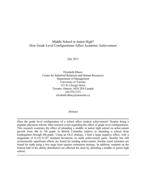
<strong>Middle</strong> <strong>School</strong> <strong>or</strong> Juni<strong>or</strong> <strong>High</strong><br />
How Grade Level Configurations Affect Academic Achievement<br />
July 2011<br />
Elizabeth Dhuey<br />
Centre f<strong>or</strong> Industrial Relations and Human Resources<br />
Department of Management<br />
University of T<strong>or</strong>onto<br />
121 St. Ge<strong>or</strong>ge Street<br />
T<strong>or</strong>onto, Ontario, M5S 2E8 Canada<br />
416.978.2721<br />
elizabeth.dhuey@ut<strong>or</strong>onto.ca<br />
Abstract<br />
Does the grade level configuration of a school affect student achievement Despite being a<br />
popular education ref<strong>or</strong>m, little research exists regarding the effect of grade level configurations.<br />
This research examines the effect of attending a middle <strong>or</strong> juni<strong>or</strong> high school on achievement<br />
growth from 4th to 7th grade in British Columbia relative to attending a school from<br />
kindergarten through 8th grade. Using an OLS strategy, I find a large negative effect, with a<br />
magnitude of 0.125–0.187 standard deviations on math achievement gains. Smaller but still<br />
economically significant effects are found f<strong>or</strong> reading achievement. Similar sized estimates are<br />
found f<strong>or</strong> math using a two stage least squares estimation strategy. In addition, students on the<br />
bottom half of the ability distribution are affected the most by attending a middle <strong>or</strong> juni<strong>or</strong> high<br />
school.
I. Introduction<br />
Over the past century, grade level configurations in schools have been in a constant state<br />
of flux—schools serving all grades transition to self-contained middle and juni<strong>or</strong> high schools,<br />
and then back again. Currently, there is a push to merge middle and juni<strong>or</strong> high schools with<br />
their elementary counterparts to create kindergarten through 8th grade schools (Schwartz et al.<br />
f<strong>or</strong>thcoming). This paper examines the effect of different grade level configurations on student<br />
achievement in British Columbia, Canada, by testing whether students who attend a middle <strong>or</strong><br />
juni<strong>or</strong> high school have different academic achievement gains from grade 4 to grade 7 than do<br />
students who attend one school from kindergarten until the beginning of high school.<br />
Understanding the impact of grade level configuration on academic achievement is<br />
imp<strong>or</strong>tant, as rearranging grade level configurations within schools may be a comparatively<br />
inexpensive policy lever compared to other school ref<strong>or</strong>ms, and it is something over which<br />
individual districts often have control. Grade level configuration may have an effect on student<br />
achievement as it can impact schools’ practices and policies such as curriculum development and<br />
delivery. It can also have an effect on school and coh<strong>or</strong>t size, and it determines the number and<br />
timing of structural transitions a student takes during his <strong>or</strong> her educational career. Finally, it can<br />
affect peer composition and age distribution within schools. All of these fact<strong>or</strong>s can greatly<br />
influence student achievement. However, despite the extensive research that has been conducted<br />
on other fact<strong>or</strong>s that may affect achievement growth—such as teacher quality, class size, and<br />
school resources—very little attention has been paid to the effect of grade level configurations.<br />
During the early 1900s in the United States, education ref<strong>or</strong>mers experimented with<br />
splitting the elementary school grades into two school types, one f<strong>or</strong> the early elementary grades<br />
and one f<strong>or</strong> the later grades, termed juni<strong>or</strong> high school. Educat<strong>or</strong>s during that time believed that<br />
1
the kindergarten through 8th grade schooling structure was unsupp<strong>or</strong>ted by psychological<br />
research and ign<strong>or</strong>ed the developmental needs of the students (Fleming and Toutant 1995).<br />
During this time period, the development of juni<strong>or</strong> high schools in Canada generally lagged<br />
behind the United States by m<strong>or</strong>e than a decade. However, by 1920, two juni<strong>or</strong> high schools<br />
opened in Canada - one in Winnipeg, Manitoba, and one in Edmonton, Alberta (Johnson 1968).<br />
British Columbia’s first juni<strong>or</strong> high school, which served grades 7 through 9, opened in<br />
Penticton, in 1926 (Fleming and Toutant 1995). By 1950, many juni<strong>or</strong> high schools existed in<br />
British Columbia, and over 5000 juni<strong>or</strong> high schools existed in the United States (Lounsbury<br />
1960). Despite this trend, the British Columbia Ministry of <strong>Education</strong> decided to return grade 7<br />
to the elementary system, and during the 1950s re<strong>or</strong>ganized all provincial schools into<br />
kindergarten through 7th grade schools, 8th through 10th grade schools, and 11th through 12th<br />
grade schools. However, even after this re<strong>or</strong>ganization the debate continued in British Columbia<br />
regarding the ―best‖ grade level configuration. In the 1960s, education ref<strong>or</strong>mers began to<br />
advocate f<strong>or</strong> middle schools—i.e., schools that started in 6th grade. By the 1980s, many middle<br />
schools existed in British Columbia. Currently, local school districts in British Columbia are<br />
allowed to determine the nature of the grade level configurations in their own district. However,<br />
the British Columbia Ministry of <strong>Education</strong> does not officially recognize institutions as middle<br />
<strong>or</strong> juni<strong>or</strong> high schools. 1<br />
I use panel data from the province of British Columbia, which has a variety of grade level<br />
configurations by district and within districts, to measure the effects of alternative grade level<br />
configurations on math and reading test sc<strong>or</strong>e gains. Approximately 16 percent of students in<br />
British Columbia attend a middle school that begins in 6th grade, and another 16 percent of<br />
1 <strong>Middle</strong> school refers to a school that starts in 6th grade, and juni<strong>or</strong> high school refers to a school that starts in 7th<br />
grade.<br />
2
students attend a juni<strong>or</strong> high school that begins in 7th grade. <strong>The</strong>ref<strong>or</strong>e, about 32 percent of<br />
students attend a stand-alone middle <strong>or</strong> juni<strong>or</strong> high school, and the other 68 percent attend a<br />
school whose grades extend through 7th grade and higher. I find that math and reading sc<strong>or</strong>es are<br />
significantly negatively affected by middle <strong>or</strong> juni<strong>or</strong> high school attendance. Specifically, I find<br />
that math sc<strong>or</strong>es of students who attended a middle <strong>or</strong> juni<strong>or</strong> high school were between 0.125–<br />
0.187 standard deviations lower than students who attended a kindergarten through 7th grade <strong>or</strong><br />
higher school, and reading sc<strong>or</strong>es were 0.055–0.108 standard deviations lower. In addition, the<br />
effect was similar between students who entered in a middle school in 6th grade and students<br />
who entered a juni<strong>or</strong> high school in 7th grade.<br />
<strong>The</strong> choice to attend middle <strong>or</strong> juni<strong>or</strong> high school in upper elementary grade levels may<br />
be endogenous and may be related to time-varying fact<strong>or</strong>s that are uncontrolled f<strong>or</strong> in this<br />
analysis. However, this may not be a large issue as students are generally restricted to attending<br />
the school in their catchment area, so the choice of schools is based on residential relocation<br />
instead of other unobservable fact<strong>or</strong>s. Nevertheless, following Rockoff and Lockwood (2010), I<br />
construct an instrumental variable using the terminal grade of the school the student attended in<br />
4th grade f<strong>or</strong> middle <strong>or</strong> juni<strong>or</strong> high school entry. <strong>The</strong> subsequent results using a two-stage least<br />
squares regression strategy find that students who attended middle <strong>or</strong> juni<strong>or</strong> high school sc<strong>or</strong>ed<br />
0.116–0.215 standard deviations lower in math than the students who did not.<br />
Finally, I find no relationship between the effect of grade level configuration and either<br />
gender, special education status, being ab<strong>or</strong>iginal, <strong>or</strong> being a student with English as a second<br />
language. However, students on the bottom half of the test sc<strong>or</strong>e distribution were<br />
disprop<strong>or</strong>tionately negatively affected by attending a middle <strong>or</strong> juni<strong>or</strong> high school.<br />
3
II. Related Literature<br />
Relatively few studies have examined the impact of grade level configuration on student<br />
achievement, despite its potential imp<strong>or</strong>tance. Earlier education w<strong>or</strong>k used cross-sectional data to<br />
examine this issue, and generally found that there was a relationship between attending middle <strong>or</strong><br />
juni<strong>or</strong> high school and lower academic perf<strong>or</strong>mance. 2 Due to the cross-sectional nature of the<br />
data, these studies were unable to conclude whether these differences were due to differences in<br />
grade level configurations <strong>or</strong> due to differences in student characteristics across these different<br />
configurations.<br />
M<strong>or</strong>e recent w<strong>or</strong>k by Cook et al. (2008) and Weiss and Kipnes (2006) examined nonacademic<br />
outcomes such as suspensions, school safety, and self-esteem. <strong>The</strong>y found lower levels<br />
of self-esteem and perceived school safety, and higher levels of student misconduct among<br />
students who attended middle schools.<br />
<strong>The</strong> research most relevant to our study includes Bedard and Do (2005), Schwartz et al.<br />
(f<strong>or</strong>thcoming), and Rockoff and Lockwood (2010). All three examine the effect of grade level<br />
configuration using longitudinal data. Bedard and Do (2005) estimated the effect on on-time high<br />
school graduation of moving from a juni<strong>or</strong> high school system, where students stay in<br />
elementary school longer, to a middle school system. <strong>The</strong>y found that moving to a middle school<br />
system decreases on-time high school graduation by 1–3 percent. Rockoff and Lockwood (2010)<br />
used a two-stage least squares approach and Schwartz et al. (f<strong>or</strong>thcoming) used an <strong>or</strong>dinary least<br />
squares approach using the same longitudinal data from New Y<strong>or</strong>k City. Both found that moving<br />
students from elementary to middle school in 6th <strong>or</strong> 7th grade causes significant drops in both<br />
math and English test sc<strong>or</strong>es.<br />
2 See, f<strong>or</strong> example, Alspaugh 1998a,b; Byrnes and Ruby 2007; Franklin and Glascock 1998; Wihry, Coladarci, and<br />
Meadow 1992.<br />
4
Using an instrumental variables estimation strategy similar to Rockoff and Lockwood<br />
(2010), this paper expl<strong>or</strong>es the issue of middle and juni<strong>or</strong> high schools in a Canadian context. In<br />
addition, this paper uses longitudinal data from an entire province versus a single city. This is an<br />
imp<strong>or</strong>tant exercise as New Y<strong>or</strong>k City has a unique educational environment, and results from<br />
that city may not be generalizable to other settings and locations. F<strong>or</strong> instance, unlike New Y<strong>or</strong>k<br />
City, British Columbia has a wide variety of urban and rural schools over a very large<br />
geographic area. In addition, the per pupil funding in New Y<strong>or</strong>k is approximately twice as large<br />
as the per pupil funding in British Columba. <strong>The</strong>se along with many other institutional<br />
differences make it imp<strong>or</strong>tant to examine the effect of grade level configurations in British<br />
Columbia.<br />
III. Methodology<br />
<strong>The</strong> analysis uses a value-added specification of achievement growth in math and reading<br />
from grade 4 to grade 7. This strategy uses the variation of grade level configurations across the<br />
province of British Columbia to estimate the effect on student achievement gains of attending a<br />
middle <strong>or</strong> juni<strong>or</strong> high school. <strong>The</strong> initial estimation strategy is as follows:<br />
y<br />
7<br />
4<br />
' ' '<br />
ist<br />
0<br />
1yist<br />
2<br />
i<br />
xit3<br />
sst4<br />
cst5<br />
M <br />
(1)<br />
ist<br />
where<br />
7<br />
yist<br />
is the grade 7 math <strong>or</strong> reading sc<strong>or</strong>e f<strong>or</strong> student i, in school s, in year t;<br />
4<br />
yist<br />
is the<br />
student’s c<strong>or</strong>responding grade 4 sc<strong>or</strong>e;<br />
M<br />
i<br />
is an indicat<strong>or</strong> equal to one if the student changed<br />
from an elementary school to a middle <strong>or</strong> juni<strong>or</strong> high school between grade 4 and grade 7;<br />
vect<strong>or</strong> of student-level demographic characteristics,<br />
and<br />
'<br />
xit<br />
is a<br />
'<br />
sst<br />
is a vect<strong>or</strong> of school-level characteristics,<br />
'<br />
c<br />
st is a vect<strong>or</strong> of community-level characteristics; and ist<br />
is an idiosyncratic err<strong>or</strong> term. In<br />
5
addition, some specifications will include city <strong>or</strong> district fixed effects because middle/juni<strong>or</strong> high<br />
school geographic locations may not be <strong>or</strong>thogonal to unobserved fact<strong>or</strong>s. <strong>The</strong>ref<strong>or</strong>e, the city <strong>or</strong><br />
district fixed effects f<strong>or</strong>ce the identifying variation to come from within a particular city <strong>or</strong><br />
district. Other specifications that allow f<strong>or</strong> differences in the effect based on whether the student<br />
attended a middle <strong>or</strong> juni<strong>or</strong> high school will be expl<strong>or</strong>ed in Section V, Part A.<br />
<strong>The</strong> coefficient of interest is <br />
2<br />
, which measures the differential effect on a student's test<br />
sc<strong>or</strong>e growth of attending a middle <strong>or</strong> juni<strong>or</strong> high school compared to staying in an elementary<br />
school from kindergarten through 7th grade <strong>or</strong> higher. This coefficient measures whether the<br />
traject<strong>or</strong>ies of student achievement from grade 4 to grade 7 f<strong>or</strong> students entering middle and<br />
juni<strong>or</strong> high schools are different than f<strong>or</strong> students who never attended a middle <strong>or</strong> juni<strong>or</strong> high<br />
school.<br />
An <strong>or</strong>dinary least squares identification strategy may not produce causal estimates<br />
because the choice to attend a middle <strong>or</strong> juni<strong>or</strong> high school in upper elementary grades may be<br />
related to time-varying fact<strong>or</strong>s that are unobservable. F<strong>or</strong> instance, a student who is currently in a<br />
kindergarten through 7th grade school may move to a middle school in 6th grade due to<br />
unobservable fact<strong>or</strong>s related to achievement such as a residential move <strong>or</strong> a family disruption.<br />
<strong>The</strong> <strong>or</strong>dinary least squares estimate would not be able to untangle the effect of moving to middle<br />
school from the effect of these fact<strong>or</strong>s.<br />
<strong>The</strong>ref<strong>or</strong>e, following Rockoff and Lockwood (2010), I created an instrument f<strong>or</strong> middle<br />
<strong>or</strong> juni<strong>or</strong> high school entry using the grade level configuration of the school attended in grade 4.<br />
If the student attends a school that ends in grade 5 <strong>or</strong> grade 6 when they are in grade 4, I create<br />
an indicat<strong>or</strong> variable that indicates the student should enter a middle <strong>or</strong> juni<strong>or</strong> high school in<br />
6
grade 6 <strong>or</strong> 7. 3 A threat to the validity of this instrument would be if the configuration of the<br />
school attended in grade 4 is related to something unobserved that affects test sc<strong>or</strong>e growth from<br />
grade 4 to grade 7 that is not controlled f<strong>or</strong> by the inclusion of the grade 4 test sc<strong>or</strong>e along with<br />
the large quantity of student, school, and community characteristics. <strong>The</strong> estimates produced<br />
using this estimation strategy can be interpreted as local average treatment effects. <strong>The</strong> estimates<br />
apply to students who are induced to move into a middle <strong>or</strong> juni<strong>or</strong> high school because they<br />
attended a school ending in grade 5 <strong>or</strong> 6. This may be very different than the average treatment<br />
effect.<br />
A possible concern with this analysis is the potential f<strong>or</strong> non-random attrition from public<br />
schools in British Columbia. This could cause a bias in an unknown direction. Only 10 percent of<br />
students in British Columbia attend private schools, but it is possible that a high-achieving child who<br />
was initially sent to a school that ended in 5th <strong>or</strong> 6th grade may be sent to a private middle school. It<br />
is also equally possible that a child who was low achieving during the early elementary years may be<br />
sent to a private middle school. <strong>The</strong>ref<strong>or</strong>e, in this analysis, a balanced panel of students who were in<br />
the public school system in British Columbia in both 4th and 7th grade is used. Hence, the<br />
interpretation of the results pertains only to those students.<br />
IV. Data and Analysis Sample<br />
A. Data Sources<br />
<strong>The</strong> main datasets used in this study were three linked files obtained from the Ministry of<br />
<strong>Education</strong> in British Columbia. <strong>The</strong> first contains observations on all students writing the Foundation<br />
3 Some schools changed their grade level configuration during this sample period. <strong>The</strong>ref<strong>or</strong>e, the instrument reflects<br />
these changes when they occur. In addition, in Section V, Part A, the analysis is broken up into whether the student<br />
attended a middle school versus a juni<strong>or</strong> high school. <strong>The</strong>ref<strong>or</strong>e, one instrument was created f<strong>or</strong> students in 4th<br />
grade whose school ended in 5th grade, and another instrument was created f<strong>or</strong> students in 4th grade whose school<br />
ended in 6th grade.<br />
7
Skills Assessment, an annual low-stakes standardized test in the areas of mathematics, reading, and<br />
writing f<strong>or</strong> students in grades 4 and 7. Data from 1999 through 2006 was used. F<strong>or</strong> these students, the<br />
percentage sc<strong>or</strong>e on each test, the school in which the test was written, and whether the student was<br />
excused from the test are known. 4 Student sc<strong>or</strong>es are linked over time via an encrypted student<br />
identifier.<br />
Student test sc<strong>or</strong>es are linked via the student identifier to the second file, which contains the<br />
administrative rec<strong>or</strong>ds of all public school students in British Columbia from 1999–2006 in grades 4<br />
to 7. <strong>The</strong>se data include demographic inf<strong>or</strong>mation such as gender, ab<strong>or</strong>iginal status, date of birth, and<br />
home language, along with inf<strong>or</strong>mation on whether they participate in special education <strong>or</strong> English as<br />
a second language (ESL) programs. Finally, the 6-digit postal code of their home residence is<br />
included. In urban areas, this is a very small area consisting sometimes of one side of a city block. In<br />
less-populated areas, it can coincide with part <strong>or</strong> all of a town.<br />
<strong>The</strong> third file contains inf<strong>or</strong>mation on all public schools in British Columbia. F<strong>or</strong> each<br />
school, the following are known: which grades are offered, the number of teachers, whether school is<br />
standard <strong>or</strong> other type, and the year of opening and/<strong>or</strong> closing. Each school’s exact address and postal<br />
code are included, which give its precise location.<br />
Data from the Canada Census is appended to this main set of files. To proxy f<strong>or</strong> student-level<br />
socioeconomic status characteristics (SES), various census variables at the<br />
Dissemination/Enumeration Area (DA) level are attached using the students’ residential postal<br />
codes. 5 DAs are relatively small areas designed to contain roughly 400–700 people, and as such act<br />
as a reasonable proxy f<strong>or</strong> a student’s SES characteristics. Inf<strong>or</strong>mation on household income,<br />
education levels, unemployment rates, ethnic and immigrant composition, and the age distribution of<br />
each DA is attached to the data.<br />
4 Students with po<strong>or</strong> English abilities and some students with severe disabilities are excused from writing provincial<br />
exams.<br />
5 This process is described in detail in a data appendix that is available from the auth<strong>or</strong> upon request.<br />
8
<strong>The</strong>ref<strong>or</strong>e, the demographic, school, and community control variables included in the<br />
analysis are dummy variables f<strong>or</strong> whether the student is male, ab<strong>or</strong>iginal, ESL, in special education,<br />
<strong>or</strong> has moved schools. Also included is the percentage in the school of male students, ab<strong>or</strong>iginal<br />
students, ESL students, special education students, students excused from the math test, and students<br />
excused from the reading test. In addition, the teacher–pupil ratio and whether the school is in a rural<br />
location are included. Finally, the census DA-level community control variables include the average<br />
household income, average dwelling value, the percentage of individuals with no high school degree,<br />
the percentage of individuals with a high school degree, the percentage of individuals with a<br />
university degree, the unemployment rate, the percentage of immigrants, the percentage of visible<br />
min<strong>or</strong>ities, and the percentage of the population over 65 years old.<br />
B. Regression Sample<br />
Because a value-added model in test sc<strong>or</strong>es is estimated, the sample is restricted to students<br />
who wrote both the 4th- and 7th-grade mathematics and reading exams. Since test sc<strong>or</strong>es were<br />
observed between 1999 and 2006, and since three years pass between each test, most such students<br />
were observed between 2002 and 2006. <strong>The</strong>re were 229,337 students observed writing the grade 7<br />
test between 2002 and 2006. Of these students, 27,286 (11.9 percent) who were not observed in all<br />
years between grades 4 and 7 were dropped from the sample, and a further 14,692 students (6.5<br />
percent) who did not have a valid test sc<strong>or</strong>e in both years were also dropped. Additionally, 657<br />
students (
C. Descriptive Statistics<br />
<strong>The</strong> summary statistics in Table 1 f<strong>or</strong> test sc<strong>or</strong>es and demographics are based on this sample<br />
of 185,170 students. Each column of Table 1 includes the sample of students who were attending<br />
schools with different grade level configurations during their 4th-grade year. Column 1 includes only<br />
students who were attending a school ending in 5th grade, column 2 includes only students who were<br />
attending a school ending in 6th grade, and column 3 includes students who were attending a school<br />
ending in 7th grade <strong>or</strong> higher.<br />
Panel A includes the descriptive statistics f<strong>or</strong> the student-level variables. <strong>The</strong> 4th-grade math<br />
and reading test sc<strong>or</strong>es are standardized to have a mean of zero and standard deviation of one in the<br />
population. <strong>The</strong> means of these test sc<strong>or</strong>es are slightly positive in all columns, which indicates that<br />
the students who were excluded from the samples sc<strong>or</strong>ed marginally w<strong>or</strong>se than the students who<br />
were included in the samples. In addition, the students who attended a school that ended in 5th grade<br />
sc<strong>or</strong>ed higher math and reading sc<strong>or</strong>es than the other students in different grade level configurations.<br />
However, a different pattern emerges f<strong>or</strong> the 7th grade test sc<strong>or</strong>es. Students in schools that<br />
ended in grade 7 <strong>or</strong> later did better in both math and reading. <strong>The</strong> students in schools that ended in<br />
grade 6—the same students who were doing better than the rest in grade 4—sc<strong>or</strong>ed lower compared<br />
to the students in column 3. This provides some indication that the analysis will find negative effects<br />
associated with attending middle <strong>or</strong> juni<strong>or</strong> high school. Finally, in terms of demographic<br />
characteristics, there are fewer ab<strong>or</strong>iginal students in schools that end in grade 5 and m<strong>or</strong>e ESL<br />
students in schools that end in grade 7 <strong>or</strong> higher.<br />
<strong>The</strong> next panel includes inf<strong>or</strong>mation about school characteristics. <strong>The</strong> number of students<br />
excused from the math and reading tests did not differ between grade level configurations. However,<br />
there does exist a difference between the percentage of schools that are rural and the pupil–teacher<br />
ratios. F<strong>or</strong> instance, 17 percent of students who attended a school that ended in grade 6 were in a<br />
rural area, whereas only 11 and 13.7 percent of students who attended a school that ended in grade 5<br />
10
and grade 7 <strong>or</strong> higher, respectively, were in a rural area. Also, the pupil–teacher ratio was higher in<br />
schools that ended in grade 7 <strong>or</strong> higher.<br />
Panel C displays the community characteristics gathered from the census f<strong>or</strong> each kind of<br />
grade level configuration. Students who attended a school that ended in grade 6 had lower household<br />
income, lower average dwelling values, and higher high school dropout rates than students from the<br />
other two grade level configurations. <strong>The</strong> other large difference between the community<br />
characteristics of the different grade level configurations is with respect to percent immigrant and<br />
percent visible min<strong>or</strong>ity. <strong>School</strong>s that ended in grade 6 had much lower percentages of both.<br />
Table 2 expl<strong>or</strong>es the summary statistics of the three estimation samples used in this research.<br />
<strong>The</strong> first column includes the full sample of 185,170 students. <strong>The</strong> second column includes only<br />
districts in which 15 percent <strong>or</strong> m<strong>or</strong>e of its students attended a middle <strong>or</strong> juni<strong>or</strong> high school. 7 <strong>The</strong><br />
third column includes only cities in which 15 percent <strong>or</strong> m<strong>or</strong>e of the students attended a middle <strong>or</strong><br />
juni<strong>or</strong> high school. 8 <strong>The</strong> second and third sample is used to limit the identification to students who<br />
had the opp<strong>or</strong>tunity to attend a middle <strong>or</strong> juni<strong>or</strong> high school. Panel A examines the test sc<strong>or</strong>es of each<br />
of these three samples. <strong>The</strong> 4th-grade test sc<strong>or</strong>es between the three samples are quite similar. This is<br />
reassuring as it implies that districts and cities that have a large number of middle and juni<strong>or</strong> high<br />
schools are not substantially different in terms of their ability to produce grade 4 test sc<strong>or</strong>es.<br />
<strong>The</strong>ref<strong>or</strong>e, the analysis can assume that the students are starting at a similar level in grade 4 in all<br />
three samples. However, a large significant difference can be seen in the 7th grade test sc<strong>or</strong>es<br />
between the three samples. This once again gives some indication that students who attend a middle<br />
7 <strong>The</strong>se districts are Southeast Kootenay, Rocky Mountain, Kootenay Lake, Kootenay-Columbia, Central Okanagan,<br />
Abbotsf<strong>or</strong>d, New Westminster, Powell River, Okanagan Similkameen, Bulkley Valley, Prince Ge<strong>or</strong>ge, Nicola-<br />
Similkameen, Peace River South, Greater Vict<strong>or</strong>ia, Sooke, Gulf Islands, Alberni, Fraser-Cascade, and Cowichan<br />
Valley.<br />
8 <strong>The</strong>se cities are Abbotsf<strong>or</strong>d, Armstrong, Castlegar, Cranbrook, Fruitvale, Hope, Lake Cowichan, Lumby, New<br />
Westminster, Pemberton, Powell River, Prince Ge<strong>or</strong>ge, Princeton, Salmon Arm, Smithers, Trail, Vict<strong>or</strong>ia, and<br />
Whistler.<br />
11
<strong>or</strong> juni<strong>or</strong> high school sc<strong>or</strong>e w<strong>or</strong>se in 7th grade than their counterparts that do not attend a middle <strong>or</strong><br />
juni<strong>or</strong> high school. Panel B provides m<strong>or</strong>e background on the distribution of the different types of<br />
grade level configurations. As previously noted, about 32 percent of students attend a middle <strong>or</strong><br />
juni<strong>or</strong> high school in British Columbia. If the sample is restricted to districts and cities that have<br />
m<strong>or</strong>e than 15 percent of their students attending a middle <strong>or</strong> juni<strong>or</strong> high school, this number increases<br />
to 63 and 58 percent, respectively. In addition, column 2 shows that there are m<strong>or</strong>e students attending<br />
juni<strong>or</strong> high school in this sample than in the sample including only cities. Figure 1 provides a visual<br />
representation of the districts and cities that contain m<strong>or</strong>e than 15 percent of students who attend a<br />
middle <strong>or</strong> juni<strong>or</strong> high school.<br />
V. Results<br />
A. Main Effects<br />
<strong>The</strong> analysis begins by estimating equation (1) using the data described in Section IV.<br />
Table 3 contains these results. Panel A includes the results from the <strong>or</strong>dinary least squares<br />
specification. All specifications include standard err<strong>or</strong>s that are clustered at the district level.<br />
Column 1 lists the estimates from a specification that includes no control variables and was run<br />
using the full sample of students in British Columbia. <strong>The</strong> point estimates indicate that students<br />
who attended a middle <strong>or</strong> juni<strong>or</strong> high school in 6th <strong>or</strong> 7th grade sc<strong>or</strong>ed 0.158 standard deviations<br />
lower than students who did not. <strong>The</strong> student, school, and census control variables are added in<br />
column 2, and the point estimates decrease slightly to -0.125 standard deviations. Because grade<br />
level configurations are determined at the district level, it is appropriate to take into account<br />
differences between districts that choose different grade level configurations. <strong>The</strong>ref<strong>or</strong>e, district<br />
fixed effects are added in column 3. Including district fixed effects does not substantially affect<br />
the estimated coefficient. Column 4 limits the sample to include only school districts that<br />
12
contained 15 percent of m<strong>or</strong>e of their students in a middle <strong>or</strong> juni<strong>or</strong> high school in 7th grade. 9<br />
This estimate is based on only students that were in districts that offered middle <strong>or</strong> juni<strong>or</strong> high<br />
schools to at least 15 percent of the student body. <strong>The</strong> point estimate f<strong>or</strong> this sample, which<br />
includes district fixed effects, is -0.141. Finally, a district may offer middle <strong>or</strong> juni<strong>or</strong> high school<br />
but only in certain cities, and the identification in the previous column may be from differences<br />
across individuals from different cities. <strong>The</strong>ref<strong>or</strong>e, the sample is again limited to include only<br />
cities in which m<strong>or</strong>e than 15 percent of the students attend a middle <strong>or</strong> juni<strong>or</strong> high school. In this<br />
specification, city fixed effects are included so that the identification comes from students within<br />
cities, rather than across cities. 10 Using this sample, I find that attending a middle <strong>or</strong> juni<strong>or</strong> high<br />
school decreases math sc<strong>or</strong>es by 0.187 standardized units. Columns 6 through 10 display the<br />
coefficients f<strong>or</strong> the reading test. Overall, the point estimates are about half the size of the math<br />
estimates. Compared to the estimates of Rockoff and Lockwood (2010) which estimated oneyear<br />
gains, the estimates in Panel A of Table 3, which are f<strong>or</strong> three-year gains, are slightly lower<br />
in magnitude but overall consistent with their findings. Schwartz et al. (f<strong>or</strong>thcoming) used a<br />
different specification, but also found estimates larger than the estimates from Panel A.<br />
<strong>The</strong> first stage of the two-stage least squares specification can be found in Panel B. As<br />
can be seen, the instrumental variable is strongly c<strong>or</strong>related with actual entry into middle <strong>or</strong><br />
juni<strong>or</strong> high school. <strong>The</strong> F-statistic ranges from 35 to 407. <strong>The</strong> coefficients in columns 1 and 2 are<br />
similar in magnitude to coefficients found in Rockoff and Lockwood (2010). <strong>The</strong> first-stage<br />
9 <strong>The</strong>se specifications include only 19 districts, so having too few clusters may be a problem. <strong>The</strong>ref<strong>or</strong>e, following<br />
Cameron and Miller (2010) and Cohen and Dupas (2010), the tables use critical values from a t G-1 distribution where<br />
G is 19 (f<strong>or</strong> each cluster). <strong>The</strong> critical values f<strong>or</strong> 1%, 5%, and 10% significance are 2.878, 2.101, and 1.734,<br />
respectively. However, Hansen (2007) has shown that the standard err<strong>or</strong>s listed in the tables, which were computed<br />
with the STATA cluster command, are reasonably good at c<strong>or</strong>recting f<strong>or</strong> serial c<strong>or</strong>relations in panels with as low as<br />
10 clusters.<br />
10 <strong>The</strong> estimates are similar if district fixed effects are included. Also, the magnitudes of the estimates are similar but<br />
are less precise if the samples include districts and cities with m<strong>or</strong>e than 25 percent of the students attending a<br />
middle <strong>or</strong> juni<strong>or</strong> high school. This is probably due to the decrease in sample size.<br />
13
esults found are consistent with the finding in Schwartz et al. (f<strong>or</strong>thcoming) that many students<br />
are ―off path‖—i.e., they don’t follow the proscribed path set by the grade level configuration in<br />
4th grade. <strong>The</strong> magnitude of the coefficient decreases when district <strong>or</strong> city fixed effects are<br />
included, but the instruments remains valid. <strong>The</strong> coefficient decreases because the average<br />
percentage of students being ―on path‖ in some districts is very low. F<strong>or</strong> instance, in District<br />
85—Vancouver Island N<strong>or</strong>th—there are 10 schools in the district: six schools that are<br />
kindergarten through 7th grade, one school that is kindergarten through 5th grade, one school<br />
that is kindergarten through 10th grade, and two schools that are 8th through 12th grade schools.<br />
<strong>The</strong> individuals attending the kindergarten through 5th grade school in 4th grade cannot follow<br />
the ―c<strong>or</strong>rect‖ path and attend a middle school as there are no middle schools in this district, so all<br />
of these students move to a kindergarten through 7th grade school <strong>or</strong> kindergarten through 10th<br />
grade school in grade 6. <strong>The</strong>ref<strong>or</strong>e, the first-stage coefficient f<strong>or</strong> this district is incredibly low. In<br />
addition, some schools change their grade level configurations during this period of time. <strong>The</strong><br />
students in these schools will be ―off-path‖ in the sense that their 4th grade school grade level<br />
configuration will not predict their school movements over time due to the change in grade level<br />
configurations. Hence, it is imp<strong>or</strong>tant to remember that the results from the two-stage least<br />
squares estimates are local average treatment effects. <strong>The</strong>y apply only to students who follow the<br />
―c<strong>or</strong>rect‖ path of schools predicted by their grade 4 grade level configuration.<br />
Panel C rep<strong>or</strong>ts the estimates from the two-stage least squares estimates. Overall, the<br />
coefficients f<strong>or</strong> math are slightly larger than the <strong>or</strong>dinary least squares estimates but continue to<br />
be statistically significant. <strong>The</strong> estimates are not statistically significant in the reading<br />
specifications when district <strong>or</strong> city fixed effects are included. Estimates from Rockoff and<br />
Lockwood (2010) found that math achievement falls by roughly 0.17 standard deviations and<br />
14
English achievement falls by 0.14–0.16 standard deviations when measured in 8th grade. <strong>The</strong><br />
yearly magnitude estimated by Rockoff and Lockwood (2010) is approximately three times<br />
larger than the effects estimated in this paper. In addition, Rockoff and Lockwood (2010) found<br />
significant results f<strong>or</strong> the English tests, whereas I find little to no statistically significant results<br />
f<strong>or</strong> the reading test sc<strong>or</strong>es once district <strong>or</strong> city fixed effects are included.<br />
B. <strong>Middle</strong> <strong>or</strong> Juni<strong>or</strong> <strong>High</strong> <strong>School</strong><br />
Next, I expl<strong>or</strong>e whether moving to a middle school in grade 6 has a different effect than<br />
moving to a juni<strong>or</strong> high school in grade 7. Table 4 has the results f<strong>or</strong> the specification that<br />
includes two dummy variables, one f<strong>or</strong> moving to a middle school in grade 6 and one f<strong>or</strong> moving<br />
to a juni<strong>or</strong> high school in grade 7. <strong>The</strong> specification is run using <strong>or</strong>dinary least squares in Panel<br />
A and two-stage least squares in Panel B. <strong>The</strong> estimates f<strong>or</strong> middle school and juni<strong>or</strong> high school<br />
are roughly the same f<strong>or</strong> both math and reading in Panel A. This implies that there might be a<br />
one-time shock to test sc<strong>or</strong>es, but that spending two years in a middle school bef<strong>or</strong>e the exam in<br />
7th grade is not necessarily w<strong>or</strong>se than spending one year in a juni<strong>or</strong> high school bef<strong>or</strong>e taking<br />
the exam. In Panel B, there exist some non-significant results f<strong>or</strong> the juni<strong>or</strong> high school<br />
coefficients f<strong>or</strong> both math and reading. <strong>The</strong>ref<strong>or</strong>e, there is some evidence of a larger negative<br />
effect f<strong>or</strong> attending middle school versus juni<strong>or</strong> high school when tested in 7th grade. This is a<br />
slightly surprising result, as the disruption of moving to a juni<strong>or</strong> high school would be fresher<br />
than if the student moved the year pri<strong>or</strong>. However, Rockoff and Lockwood (2010) found a<br />
similar pattern using New Y<strong>or</strong>k City data. In addition, Cook et al. (2008) came to a similar<br />
conclusion regarding discipline problems using N<strong>or</strong>th Carolina data, and hypothesized that<br />
younger students may be m<strong>or</strong>e sensitive to the negative influences of older students.<br />
15
C. Heterogeneous Effects<br />
Table 5 expl<strong>or</strong>es whether the negative effect of attending middle and juni<strong>or</strong> high school<br />
varies by different demographic characteristics. Panel A examines gender by interacting an<br />
indicat<strong>or</strong> variable f<strong>or</strong> male with the middle/juni<strong>or</strong> high school indicat<strong>or</strong> variable. Each test and<br />
estimation strategy includes results f<strong>or</strong> three different samples/specifications. <strong>The</strong> first column<br />
c<strong>or</strong>responds to the third column in Table 3 and Table 4. It includes the entire sample along with<br />
district fixed effects. Column 2 c<strong>or</strong>responds to the sample of only districts with 15 percent <strong>or</strong><br />
greater of students attending a middle <strong>or</strong> juni<strong>or</strong> high school along with district fixed effects.<br />
Column 3 includes cities with 15 percent <strong>or</strong> greater of students attending a middle <strong>or</strong> juni<strong>or</strong> high<br />
school along with city fixed effects. <strong>The</strong>se three columns are repeated f<strong>or</strong> the reading test and f<strong>or</strong><br />
the math and reading test results using two-stage least squares. Overall, there is very little<br />
evidence that males are affected differently than females. <strong>The</strong> same is true f<strong>or</strong> students in special<br />
education (Panel B), ab<strong>or</strong>iginal students (Panel C), and ESL students (Panel D). However, Panel<br />
E includes an indicat<strong>or</strong> f<strong>or</strong> whether the student sc<strong>or</strong>ed in the lowest 50 percent of test takers in<br />
4th grade. This indicat<strong>or</strong> is interacted with the middle/juni<strong>or</strong> high school variable. Here we see a<br />
very large negative effect f<strong>or</strong> those on the lower half of the ability distribution. In particular, in<br />
reading, the whole effect is driven by these lower achieving students. <strong>The</strong>se findings c<strong>or</strong>respond<br />
to those of Rockoff and Lockwood (2010) but have some dissimilarities with those of Schwartz<br />
et al. (f<strong>or</strong>thcoming) as they found no differential impacts f<strong>or</strong> females, special education students,<br />
<strong>or</strong> limited English proficiency-eligible students in math. <strong>The</strong>y did, however, find large positive<br />
effects f<strong>or</strong> limited English proficiency-eligible students in reading. I find no heterogeneous<br />
effects in reading f<strong>or</strong> ESL students. <strong>The</strong>se differences may be due to differences in the programs<br />
available to the ESL students in these two locations.<br />
16
D. Moving <strong>or</strong> <strong>Middle</strong>/Juni<strong>or</strong> <strong>High</strong> <strong>School</strong><br />
A possible interpretation of these findings is that the effects found have only to do with<br />
the act of moving schools and nothing to do with attending a particular type of grade level<br />
configuration. <strong>The</strong> literature generally finds negative effects of moving schools on the student’s<br />
academic achievement (see Engec 2006; Gruman et al. 2008; Ingersoll et al. 1989; Mehana and<br />
Reynolds 2004). However, it is difficult to separate whether this negative effect is due to the act<br />
of moving <strong>or</strong> due to the characteristics and circumstances of the students who move. <strong>The</strong>ref<strong>or</strong>e,<br />
is it difficult to disentangle whether the results found above are due to simply moving schools<br />
versus moving to a middle <strong>or</strong> juni<strong>or</strong> high school.<br />
Ideally, one could find an exogenous reason f<strong>or</strong> students to move schools and then<br />
compare the effects of moving schools f<strong>or</strong> those students with the effect of moving to a middle<br />
<strong>or</strong> juni<strong>or</strong> high school. Unf<strong>or</strong>tunately, finding an exogenous reason is difficult in these particular<br />
data. However, in Table 6, I expl<strong>or</strong>e the test sc<strong>or</strong>e effects of moving f<strong>or</strong> two different samples of<br />
movers. In Panel A, an indicat<strong>or</strong> variable is used that equals one f<strong>or</strong> all students who moved<br />
schools during this sample whose move was not related to attending a middle <strong>or</strong> juni<strong>or</strong> high<br />
school. <strong>The</strong> point estimates indicate a negative relationship between changing schools and test<br />
sc<strong>or</strong>e gains from grade 4 to grade 7. <strong>The</strong> magnitude is between one-third and one-half as large as<br />
the negative effects found f<strong>or</strong> middle/juni<strong>or</strong> high school attendance. However, this sample of<br />
students may be negatively academically selected to start with (Pribesh and Downey 1999). It<br />
may be that these students are likely to do w<strong>or</strong>se than other students in terms of academic gains<br />
due to other unobservable characteristics. However, it is interesting that the c<strong>or</strong>relation is much<br />
smaller than the point estimates found f<strong>or</strong> middle/juni<strong>or</strong> high school attendance.<br />
Starting in 2000, many schools were closed in British Columbia due to decreasing student<br />
enrolments. In this sample, 56 schools closed between 2000 and 2005. In Panel B, I use the<br />
17
students that were f<strong>or</strong>ced to move schools due to school closure to estimate the effect of mobility<br />
on test sc<strong>or</strong>e gains. <strong>The</strong> school closures were not exogenous events, as the schools were selected<br />
to be closed due to decreasing enrolments, and this may have been c<strong>or</strong>related with other<br />
unobserved fact<strong>or</strong>s. However, this is still inf<strong>or</strong>mative as it may remove some of the selection into<br />
the movers’ sample found in Panel A. Interestingly, moving schools due to school closures did<br />
not have any statistically significant effect on students’ test sc<strong>or</strong>e gains in math <strong>or</strong> reading.<br />
Neither Panel A n<strong>or</strong> Panel B shows conclusive evidence of whether the effects found in<br />
this research are due to moving schools versus moving to a middle <strong>or</strong> juni<strong>or</strong> high school.<br />
However, they do show suggestive evidence that the move to middle <strong>or</strong> juni<strong>or</strong> high school may<br />
be significantly w<strong>or</strong>se on student achievement gains than just changing schools during the<br />
elementary years.<br />
VI. Conclusion<br />
Overall, I find large, statistically significant negative effects of attending a middle <strong>or</strong><br />
juni<strong>or</strong> high school. <strong>The</strong> magnitudes are similar to other education interventions such as<br />
improving a teacher by one standard deviation (Aaronson, Barrow, and Sander 2007), the black–<br />
white test sc<strong>or</strong>e gap (Fryer and Levitt 2006), <strong>or</strong> reducing class sizes (Harris 2009). <strong>The</strong> large<br />
effect size and the potential easy policy ref<strong>or</strong>m make changing grade level configurations an<br />
imp<strong>or</strong>tant and viable education ref<strong>or</strong>m. <strong>The</strong> adoption of a kindergarten through 8th grade<br />
configuration is becoming m<strong>or</strong>e popular with a variety of U.S. school districts that are moving in<br />
that direction, such as New Y<strong>or</strong>k City, Cleveland, Cincinnati, Philadelphia, and Boston<br />
(Schwartz et al. f<strong>or</strong>thcoming). This research shows that this re<strong>or</strong>ganization may be quite<br />
18
eneficial and that British Columbia school districts may want to rethink their grade level<br />
configuration options.<br />
Despite the consistent and large effects found in this research, it is still unclear exactly<br />
what is causing the negative effect of middle and juni<strong>or</strong> high school attendance. Is it the grade<br />
distribution of the students in the school Are middle/juni<strong>or</strong> high schools less efficient Do the<br />
peer effects matter <strong>The</strong>se are all questions that cannot be answered with these data but that are<br />
imp<strong>or</strong>tant f<strong>or</strong> future research.<br />
VII. References<br />
Aaronson, D., L. Barrow, and W. Sander (2007) "Teachers and student achievement<br />
in the Chicago public high schools," Journal of Lab<strong>or</strong> Economics 25(1), 95–135<br />
Alspaugh, J.W. (1998a) ―Achievement loss associated with the transition to middle school and<br />
high school,‖ <strong>The</strong> Journal of <strong>Education</strong>al Research 92(1), 20–25<br />
Alspaugh, J.W. (1998b) ―<strong>The</strong> relationship of school-to-school transitions and school size to high<br />
school dropout rates,‖ <strong>High</strong> <strong>School</strong> Journal 81(3), 154–160<br />
Bedard, K., and C. Do (2005) ―Are middle schools m<strong>or</strong>e effective <strong>The</strong> impact of school<br />
structure on student outcomes,‖ <strong>The</strong> Journal of Human Resources 40(3), 660–82<br />
Byrnes, V., and A. Ruby (2007) ―Comparing achievement between K–8 and middle schools: A<br />
large-scale empirical study,‖ American Journal of <strong>Education</strong> 114(1), 101–35<br />
Cameron, C.A., and D.L. Miller (2010) Robust Inference with Clustered Data, W<strong>or</strong>king Paper<br />
10-7. Department of Economics, University of Calif<strong>or</strong>nia – Davis<br />
Cohen, J., and P. Dupas (2010) "Free distribution <strong>or</strong> cost-sharing Evidence from a randomized<br />
malaria prevention experiment," Quarterly Journal of Economics 125(1), 1-45<br />
Cook, P. J., R. MacCoun, C. Muschkin, and J. Vigd<strong>or</strong> (2008) ―<strong>The</strong> negative impacts of starting<br />
middle school in 6th grade,‖ Journal of Policy Analysis and Management 27(1), 104–21<br />
Engec, N. (2006) ―<strong>The</strong> relationship between mobility and student perf<strong>or</strong>mance and behavi<strong>or</strong>,‖<br />
Journal of <strong>Education</strong>al Research 99(3), 167-78<br />
19
Fleming, T., and T. Toutant (1995) ―Redefining the time to transition: A hist<strong>or</strong>y of juni<strong>or</strong> high<br />
school movements in British Columbia,‖ <strong>Education</strong> Canada 30-37<br />
Franklin, B.J., and C.H. Glascock (1998) ―<strong>The</strong> relationship between grade configuration and<br />
student perf<strong>or</strong>mance in rural schools,‖ Journal of Research in Rural <strong>Education</strong> 14(3), 149<br />
Fryer, R.G., and S.D. Levitt (2006) "<strong>The</strong> black-white test sc<strong>or</strong>e gap through third grade,"<br />
American Law and Economics Review 8(2), 249-81<br />
Gruman, D.H., T.W. Harachi, R.D. Abbott, R.F. Catalano, and C.B. Fleming (2008)<br />
―Longitudinal effects of student mobility on three dimensions of elementary school<br />
engagement,‖ Child Development 79(6), 1833–52<br />
Hansen, C.B. (2007) ―Generalized least squares inference in panel and multilevel models with<br />
serial c<strong>or</strong>relations and fixed effects,‖ Journal of Econometrics 140, 670-94<br />
Harris, D.N. (2009) ―Toward policy-relevant benchmarks f<strong>or</strong> interpreting effect sizes: combining<br />
effects with costs,‖ <strong>Education</strong>al Evaluation and Policy Analysis 31(1), 3-29<br />
Ingersoll, G., J. Scamman, and W. Eckerling (1989) ―Geographic mobility and student<br />
achievement in an urban setting,‖ <strong>Education</strong>al Evaluation and Policy Analysis 11(2), 143-49<br />
Johnson, F.H. (1968) A Brief Hist<strong>or</strong>y of Canadian <strong>Education</strong> (T<strong>or</strong>onto: McGraw-Hill)<br />
Lounsbury, J.H. (1960) "How the juni<strong>or</strong> high school came to be," <strong>Education</strong>al<br />
Leadership 18, 145-47<br />
Mehana, M., and A.J. Reynolds (2004) ―<strong>School</strong> mobility and achievement: A meta-analysis,‖<br />
Children and Youth Services Review 26(1), 93-119<br />
Pribesh, S., and D. Downey (1999) ―Why are residential and school moves associated with po<strong>or</strong><br />
school perf<strong>or</strong>mance‖ Demography 36(4), 521-34<br />
Rockoff, J., and B.B. Lockwood (2010) "Stuck in the middle: Impacts of grade configuration in<br />
public schools," Journal of Public Economics 94, 1051-61<br />
Schwartz, A.E., L. Stiefal, R. Rubenstein, and J. Zabel (f<strong>or</strong>thcoming) ―<strong>The</strong> path not taken: How<br />
does school <strong>or</strong>ganization affect eighth-grade achievement‖ <strong>Education</strong>al Evaluation and Policy<br />
Analysis<br />
Weiss, C.C., and L. Kipnes (2006) ―Re-examining middle school effects: A comparison of<br />
middle grades students in middle schools and K–8 schools,‖ American Journal of <strong>Education</strong><br />
112(2), 239–72<br />
20
Wihry, D. F., T. Coladarci, and C. Meadow (1992) ―Grade span and 8th-grade academic<br />
achievement: Evidence from a predominantly rural state,‖ Journal of Research in Rural<br />
<strong>Education</strong> 8(2), 58-70<br />
21
Table 1<br />
Descriptive statistics of student, school, and community characteristics<br />
Ending grade of school, Grade 4<br />
Grade 5 Grade 6 Grade 7 <strong>or</strong> later<br />
Mean Mean Mean<br />
(Std. Dev.) (Std. Dev.) (Std. Dev.)<br />
Panel A: Student characteristics<br />
Grade 4 math test sc<strong>or</strong>es 0.183 0.031 0.053<br />
(0.905) (0.896) (0.931)<br />
Grade 4 reading test sc<strong>or</strong>es 0.146 0.071 0.063<br />
(0.861) (0.876) (0.904)<br />
Grade 7 math test sc<strong>or</strong>es -0.017 -0.132 0.047<br />
(0.907) (0.880) (0.951)<br />
Grade 7 reading test sc<strong>or</strong>es 0.073 -0.003 0.071<br />
(0.884) (0.904) (0.913)<br />
Male 0.509 0.498 0.504<br />
(0.500) (0.500) (0.500)<br />
Ab<strong>or</strong>iginal 0.079 0.139 0.103<br />
(0.270) (0.346) (0.304)<br />
ESL 0.168 0.060 0.245<br />
(0.374) (0.237) (0.430)<br />
In special education 0.065 0.061 0.058<br />
(0.247) (0.240) (0.234)<br />
Panel B: <strong>School</strong> characteristics<br />
Number excused from math test 0.030 0.031 0.038<br />
(0.041) (0.043) (0.049)<br />
Number excused from reading test 0.030 0.031 0.039<br />
(0.041) (0.044) (0.050)<br />
Rural 0.110 0.171 0.137<br />
(0.312) (0.376) (0.344)<br />
Pupil/teacher ratio 14.310 14.118 15.591<br />
(3.080) (3.443) (2.602)<br />
Panel C: Community characteristics<br />
Average household income 56553 49547 57242<br />
(18072) (15984) (22725)<br />
Average dwelling value 232170 185686 248776<br />
(97016) (99618) (133107)<br />
% no high school degree 0.228 0.271 0.258<br />
(0.095) (0.096) (0.108)<br />
% high school degree 0.268 0.266 0.265<br />
(0.061) (0.063) (0.057)<br />
% university degree 0.196 0.144 0.197<br />
(0.102) (0.076) (0.116)<br />
% unemployed 0.063 0.078 0.072<br />
(0.047) (0.060) (0.057)<br />
% immigrant 0.239 0.131 0.263<br />
(0.134) (0.059) (0.174)<br />
% visible min<strong>or</strong>ity 0.169 0.044 0.231<br />
(0.181) (0.053) (0.249)<br />
% of population over 65 yrs old 0.132 0.138 0.120<br />
(0.102) (0.098) (0.088)<br />
Number of Observations 24,257 25,241 135,672<br />
Notes: Test sc<strong>or</strong>es represent the z-sc<strong>or</strong>e by year, grade, and skill among the population of schools pri<strong>or</strong> to sample<br />
exclusions.
Table 2<br />
Descriptive statistics of test sc<strong>or</strong>es and grade configurations f<strong>or</strong> estimation samples<br />
All districts/cities<br />
in British<br />
Columbia<br />
Only districts<br />
with > 15% of<br />
students in<br />
middle schools<br />
Only cities with<br />
> 15% of<br />
students in<br />
middle schools<br />
Mean Mean Mean<br />
(Std. Dev.) (Std. Dev.) (Std. Dev.)<br />
Panel A: Test Sc<strong>or</strong>es<br />
Grade 4 math test sc<strong>or</strong>es 0.067 0.034 0.066<br />
(0.924) (0.908) (0.914)<br />
Grade 4 reading test sc<strong>or</strong>es 0.075 0.069 0.090<br />
(0.896) (0.891) (0.887)<br />
Grade 7 math test sc<strong>or</strong>es 0.014 -0.078 -0.038<br />
(0.938) (0.916) (0.930)<br />
Grade 7 reading test sc<strong>or</strong>es 0.061 0.021 0.042<br />
(0.908) (0.919) (0.924)<br />
Panel B: Grade Configurations<br />
<strong>Middle</strong>/juni<strong>or</strong> high school 0.317 0.630 0.582<br />
(0.465) (0.483) (0.493)<br />
<strong>Middle</strong> school in 6th grade 0.162 0.255 0.356<br />
(0.369) (0.436) (0.479)<br />
Juni<strong>or</strong> high school in 7th grade 0.157 0.382 0.232<br />
(0.364) (0.486) (0.422)<br />
Number of Observations 185,170 47,264 29,935<br />
Notes: Test sc<strong>or</strong>es represent the z-sc<strong>or</strong>e by year, grade, and skill among the population of schools pri<strong>or</strong> to<br />
sample exclusions.
Table 3<br />
Ordinary least squares estimates of the effect of middle and juni<strong>or</strong> high school on academic gains<br />
Math<br />
Reading<br />
(1) (2) (3) (4) (5) (6) (7) (8) (9) (10)<br />
Panel A: OLS<br />
<strong>Middle</strong>/juni<strong>or</strong> high school -0.158 -0.125 -0.130 -0.141 -0.187 -0.056 -0.065 -0.055 -0.079 -0.108<br />
(0.033) (0.027) (0.030) (0.031) (0.029) (0.018) (0.016) (0.028) (0.023) (0.026)<br />
Panel B: First stage<br />
Grade 4 0.776 0.697 0.294 0.359 0.341 0.781 0.697 0.294 0.359 0.341<br />
(0.003) (0.004) (0.005) (0.011) (0.013) (0.003) (0.004) (0.005) (0.011) (0.013)<br />
Panel C: 2SLS<br />
<strong>Middle</strong>/juni<strong>or</strong> high school -0.192 -0.147 -0.138 -0.116 -0.215 -0.077 -0.082 -0.062 -0.051 -0.085<br />
(0.036) (0.029) (0.049) (0.059) (0.057) (0.022) (0.019) (0.039) (0.049) (0.062)<br />
Number of obs 185170 185170 185170 47264 29935 185170 185170 185170 47264 29935<br />
Control variables:<br />
Student/school/census no yes yes yes yes no yes yes yes yes<br />
District fixed effects no no yes yes no no no yes yes no<br />
City fixed effects no no no no yes no no no no yes<br />
Sample:<br />
Full sample yes yes yes no no yes yes yes no no<br />
Only districts > 15% no no no yes no no no no yes no<br />
Only cities > 15% no no no no yes no no no no yes<br />
Standard err<strong>or</strong>s c<strong>or</strong>rected f<strong>or</strong> clustering at the district level are in parentheses. Critical values f<strong>or</strong> columns 4, 5, 9 & 10 are from a t-distribution<br />
with 18 degrees of freedom. Bold coefficients are statistically significant at the 5% level. Bold italic coefficients are statistically significant<br />
at the 10% level. See Section IV f<strong>or</strong> a description of the demographic and census variables included in the regressions. <strong>The</strong> F-statistic f<strong>or</strong> the<br />
first stage regressions range from 35 to 407.
Table 4<br />
OLS and instrumental variables student level estimates of school structure changes<br />
Math<br />
Reading<br />
(1) (2) (3) (4) (5) (6) (7) (8) (9) (10)<br />
Panel A: OLS<br />
<strong>Middle</strong> school grade 6 -0.130 -0.125 -0.146 -0.148 -0.179 -0.028 -0.053 -0.057 -0.078 -0.090<br />
(0.034) (0.035) (0.029) (0.033) (0.027) (0.017) (0.020) (0.026) (0.026) (0.032)<br />
Juni<strong>or</strong> high school grade 7 -0.185 -0.123 -0.113 -0.123 -0.185 -0.086 -0.079 -0.055 -0.073 -0.128<br />
(0.033) (0.027) (0.039) (0.040) (0.042) (0.022) (0.021) (0.036) (0.031) (0.027)<br />
Panel B: 2SLS<br />
<strong>Middle</strong> school grade 6 -0.166 -0.162 -0.178 -0.166 -0.208 -0.051 -0.079 -0.086 -0.079 -0.064<br />
(0.036) (0.032) (0.050) (0.063) (0.057) (0.022) (0.021) (0.031) (0.039) (0.055)<br />
Juni<strong>or</strong> high school grade 7 -0.217 -0.125 -0.038 -0.023 -0.178 -0.101 -0.080 0.009 0.006 -0.106<br />
(0.040) (0.034) (0.054) (0.063) (0.078) (0.024) (0.027) (0.064) (0.069) (0.110)<br />
Number of obs 185170 185170 185170 47264 29935 185170 185170 185170 47264 29935<br />
Control variables:<br />
Student/school/census no yes yes yes yes no yes yes yes yes<br />
District fixed effects no no yes yes no no no yes yes no<br />
City fixed effects no no no no yes no no no no yes<br />
Sample:<br />
Full sample yes yes yes no no yes yes yes no no<br />
Only districts > 15% no no no yes no no no no yes no<br />
Only cities > 15% no no no no yes no no no no yes<br />
Standard err<strong>or</strong>s c<strong>or</strong>rected f<strong>or</strong> clustering at the district level are in parentheses. Critical values f<strong>or</strong> columns 4, 5, 9 & 10 are from a t-distribution<br />
with 18 degrees of freedom. Bold coefficients are statistically significant at the 5% level. Bold italic coefficients are statistically significant at<br />
the 10% level. See Section IV f<strong>or</strong> a description of the demographic and census variables included in the regressions.
Table 5<br />
OLS student level estimates of school structure changes by demographic characteristics<br />
OLS<br />
2SLS<br />
Math Reading Math Reading<br />
(1) (2) (3) (4) (5) (6) (7) (8) (9) (10) (11) (12)<br />
Panel A: Male<br />
<strong>Middle</strong>/juni<strong>or</strong> high school -0.130 -0.149 -0.198 -0.050 -0.083 -0.107 -0.143 -0.143 -0.266 -0.058 -0.062 -0.098<br />
(0.031) (0.033) (0.029) (0.028) (0.024) (0.028) (0.049) (0.060) (0.060) (0.039) (0.046) (0.057)<br />
<strong>Middle</strong>/juni<strong>or</strong> school * male -0.002 0.016 0.023 -0.011 0.008 -0.002 0.010 0.055 0.100 -0.007 0.023 0.025<br />
(0.009) (0.014) (0.016) (0.010) (0.012) (0.013) (0.012) (0.027) (0.058) (0.013) (0.029) (0.057)<br />
Panel B: Special education<br />
<strong>Middle</strong>/juni<strong>or</strong> high school -0.131 -0.143 -0.189 -0.055 -0.082 -0.113 -0.141 -0.121 -0.219 -0.063 -0.057 -0.096<br />
(0.030) (0.031) (0.029) (0.028) (0.024) (0.027) (0.049) (0.060) (0.059) (0.039) (0.048) (0.061)<br />
<strong>Middle</strong>/juni<strong>or</strong> school * special education 0.018 0.043 0.042 -0.004 0.054 0.085 0.044 0.094 0.086 0.015 0.122 0.220<br />
(0.020) (0.028) (0.028) (0.023) (0.045) (0.050) (0.027) (0.070) (0.094) (0.030) (0.080) (0.096)<br />
Panel C: Ab<strong>or</strong>ginal<br />
<strong>Middle</strong>/juni<strong>or</strong> high school -0.131 -0.141 -0.190 -0.053 -0.077 -0.115 -0.138 -0.113 -0.210 -0.056 -0.036 -0.084<br />
(0.030) (0.032) (0.030) (0.028) (0.023) (0.025) (0.049) (0.061) (0.061) (0.038) (0.047) (0.066)<br />
<strong>Middle</strong>/juni<strong>or</strong> school * ab<strong>or</strong>iginal 0.004 -0.001 0.028 -0.015 -0.011 0.061 -0.005 -0.023 -0.041 -0.046 -0.113 -0.013<br />
(0.025) (0.040) (0.041) (0.028) (0.040) (0.038) (0.032) (0.063) (0.081) (0.037) (0.080) (0.092)<br />
Panel D: ESL<br />
<strong>Middle</strong>/juni<strong>or</strong> high school -0.131 -0.137 -0.188 -0.055 -0.072 -0.104 -0.139 -0.096 -0.187 -0.062 -0.036 -0.060<br />
(0.031) (0.030) (0.030) (0.028) (0.024) (0.027) (0.050) (0.053) (0.047) (0.039) (0.044) (0.060)<br />
<strong>Middle</strong>/juni<strong>or</strong> school * ESL 0.008 -0.038 0.011 0.001 -0.066 -0.032 0.010 -0.207 -0.193 0.005 -0.156 -0.175<br />
(0.068) (0.058) (0.067) (0.059) (0.041) (0.045) (0.076) (0.123) (0.156) (0.065) (0.134) (0.166)<br />
Panel E: Low 4th grade sc<strong>or</strong>es<br />
<strong>Middle</strong>/juni<strong>or</strong> high school -0.101 -0.091 -0.149 0.050 0.038 -0.013 -0.101 -0.046 -0.154 0.053 0.085 0.032<br />
(0.031) (0.033) (0.030) (0.029) (0.029) (0.028) (0.053) (0.066) (0.067) (0.040) (0.052) (0.071)<br />
<strong>Middle</strong>/juni<strong>or</strong> school * low sc<strong>or</strong>e -0.057 -0.100 -0.076 -0.184 -0.205 -0.171 -0.078 -0.140 -0.127 -0.216 -0.240 -0.230<br />
(0.013) (0.015) (0.016) (0.009) (0.012) (0.012) (0.017) (0.027) (0.043) (0.016) (0.019) (0.044)<br />
Number of obs 185170 47264 29935 185170 47264 29935 185170 47264 29935 185170 47264 29935<br />
Control variables:<br />
Student/school/census variables yes yes yes yes yes yes yes yes yes yes yes yes<br />
District fixed effects yes yes no yes yes no yes yes no yes yes no<br />
City fixed effects no no yes no no yes no no yes no no yes<br />
Sample:<br />
Full sample yes no no yes no no yes no no yes no no<br />
Only districts > 15% no yes no no yes no no yes no no yes no<br />
Only cities > 15% no no yes no no yes no no yes no no yes<br />
Standard err<strong>or</strong>s c<strong>or</strong>rected f<strong>or</strong> clustering at the district level are in parentheses. Critical values f<strong>or</strong> all columns except columns 1, 4, 7, & 10 are from a t-distribution with 18 degrees of<br />
freedom. Bold coefficients are statistically significant at the 5% level. Bold italic coefficients are statistically significant at the 10% level. See Section IV f<strong>or</strong> a description of the demographic<br />
and census variables included in the regressions.
Table 6<br />
Effect of moving schools on test sc<strong>or</strong>e gains from grade 4 to grade 7<br />
Math<br />
Reading<br />
(1) (2) (3) (4) (5) (6)<br />
Panel A: Movers<br />
Changed schools -0.057 -0.038 -0.050 -0.047 -0.044 -0.051<br />
(0.008) (0.010) (0.014) (0.008) (0.012) (0.017)<br />
Panel B: Movers due to school closing<br />
Changed schools 0.031 0.026 0.038 0.029 0.015 0.043<br />
(0.019) (0.022) (0.031) (0.017) (0.025) (0.035)<br />
Number of obs 185170 47264 29935 185170 47264 29935<br />
Control variables:<br />
Student/school/census variables yes yes yes yes yes yes<br />
District fixed effects yes yes no yes yes no<br />
City fixed effects no no yes no no yes<br />
Sample:<br />
Full sample yes no no yes no no<br />
Only districts > 15% no yes no no yes no<br />
Only cities > 15% no no yes no no yes<br />
Standard err<strong>or</strong>s c<strong>or</strong>rected f<strong>or</strong> clustering at the district level are in parentheses. Critical values f<strong>or</strong> columns 2, 3, 5 & 6<br />
are from a t-distribution with 18 degrees of freedom. Bold coefficients are statistically significant at the 5% level. Bold<br />
italic coefficients are statistically significant at the 10% level. See Section IV f<strong>or</strong> a description of the demographic<br />
and census variables included in the regressions.
Figure 1: British Columbia<br />
<strong>School</strong> Districts and Cities<br />
with m<strong>or</strong>e than 15% of Students<br />
Attending <strong>Middle</strong> <strong>or</strong> Juni<strong>or</strong> <strong>High</strong> <strong>School</strong><br />
!<br />
!<br />
<strong>School</strong> Districts<br />
(% of students attending<br />
middle <strong>or</strong> juni<strong>or</strong> high school)<br />
Cities<br />
!<br />
m<strong>or</strong>e than 15<br />
up to 15<br />
m<strong>or</strong>e than 15% of students attend<br />
middle <strong>or</strong> juni<strong>or</strong> high school<br />
!<br />
!<br />
!<br />
!<br />
!<br />
!<br />
!<br />
!<br />
!<br />
!<br />
!<br />
!<br />
!<br />
!<br />
!