Does it pay to pay teachers more? - The Association for Education ...

Does it pay to pay teachers more? Evidence from Oklahoma’sminimum salary scheduleMatthew D. Hendricks ∗March 8, 2012DO NOT CITE WITHOUT AUTHOR’S PERMISSIONAbstractSurprisingly little is known about how teacher salaries are causally related to educationquality. Conventional wisdom suggests that higher-paying districts will likely operate moreefficiently by reducing teacher turnover. In addition, standard theories in labor economicssuggest that higher wages may provide an incentive for teachers to work harder and may allowdistricts to attract and retain better teachers. While the potential for a relationship exists, priorempirical research has not generally supported the hypothesis that higher teacher pay bringsthe benefit of improved education quality. In this study I revisit this question with the benefitof more detailed data and a more robust estimation strategy.Public education is expensive. Each year in the United States federal, state, and local governmentsdole out billions of dollars to fund education. For the 2009-010 school year the NationalCenter for Education Statistics projects that about $602 billion was spent to support public elementaryand secondary schools (Snyder & Dillow 2011). The financial burden is particularly highat the local and state levels, which provide about 43.5% and 48.3% percent of funds respectively(Snyder & Dillow 2011). In total, state and local governments allocate about a quarter of theircombined budgets to support public K-12 education (Snyder & Dillow 2011).While education funding accounts for a large proportion of public dollars spent, especially atthe state and local levels, little is known about how education funding and allocations are relatedto education quality. In particular, surprisingly little is known about how teacher’s salaries impactquality, despite the fact that teacher’s salaries account for about 35% of current K-12 funding∗ The University of Tulsa, 800 South Tucker Drive Tulsa OK 74104, matthew-hendricks@utulsa.edu.1

(Snyder & Dillow 2011). Conventional wisdom suggests that districts that pay more will likelyattract and retain better teachers. However, prior research has not clearly supported this idea. Partof the explanation for the lack of clarity stems from the fact that it is difficult to estimate the causaleffect of teacher salaries on education quality. In order to estimate this causal relationship onemust adequately control for factors that influence education quality and are correlated with teachersalaries, which is not easily accomplished in observational studies.Given the size of the public investment and stakes involved in improving the quality of education,we ought to know whether current teacher salaries are ideal or can be altered in some way thatcan improve quality. If administrators moved funds away from teacher salaries and into other areas,such as administrator salaries, books, computers, and facilities, would quality improve? Alternatively,might teacher salaries be too low? That is, would increasing teacher salaries at the expenseof other areas of education finance cause overall quality to improve? These are important policyquestions that we can begin to answer if we measure the relationship between teacher salaries andeducation quality.Using a robust estimation strategy that relies on detailed district data and state-imposed variationin teacher salary, this study aims to measure the causal effect of public school teacher salarieson the quality of public education. I estimate the effect of teacher salaries in Oklahoma on the followingdistrict-level outcome measures: average student test scores, student drop-out rates, annualteacher turnover rates, and the characteristics of new teacher hires.Preliminary results suggest that large increases in Oklahoma’s state minimum teacher salaryschedule in 2007 and 2008 significantly reduced teacher turnover. These results are preliminary.Please do not cite without author’s permission.This work is organized as follows: section 1 provides a brief review of the literature; section2 discusses the theoretical linkage between teacher pay and teacher quality; section 3 details theempirical model and describes the data; section 4 presents the results; section 5 discusses theimplications of the findings.2

1 Literature reviewThere are several strands of literature that are relevant to this research. One strand asks whetherteachers matter. The question is whether kids who are assigned to a poor teacher perform worsethan kids assigned to a good teacher. The answer to this question seems obvious, but only recentlyhave researchers been able to objectively measure variation in teacher performance. Several studieshave confirmed that there is significant variation in teacher effectiveness, where effectiveness ismeasured by the teacher’s average contribution to student achievement growth (Hanushek & Rivkin2010, Rockoff 2004, Kane & Staiger 2008, Rothstein 2010, Kane, Rockoff & Staiger 2008, Jacob& Lefgren 2008). These studies suggest that there may be significant variation in teacher quality,even within a school.Given the potentially large disparity between effective and poor teachers, another strand ofliterature asks how districts or schools might attract the best teachers. An obvious policy instrumentis teacher salary. Holding all else constant, one might expect that if a district increases teachersalaries, then it might attract higher-ability individuals who might have otherwise chosen a higherpayingprofession outside of teaching or a position at a competing district. This logic motivates thisresearch and has been the motivation behind other similar studies that attempt to find a relationshipbetween teacher pay and student outcomes.In this area, direct evidence of a link between teacher pay and student achievement is mixed.Loeb & Page (2000) find evidence that increased teacher salaries cause a reduction in studentdropout rates and an increase in college enrollment. However, Hanushek et al. (2005) find noevidence that higher-paying districts are able to attract and hire the best teachers away from otherlow-paying districts. In a survey of the literature prior to 1995, Hanushek et al. (2004) show thatout of 118 estimates of the relationship between teacher salaries and student achievement, only20% were positive and significant, 7% were negative and significant, and 73% were insignificant.Out of the subset of student-level value-added estimates, where the analysis was restricted to asingle state, the evidence reported by Hanushek et al. (2004) is still weak: out of 17 estimates,only 3 reported a positive and statistically significant relationship between teacher salaries and3

student achievement. In all, there is little prior evidence linking teacher salaries directly to studentachievement.Another strand of literature has had success in establishing indirect links between teacher payand student outcomes. For example, evidence suggests that that higher teacher pay can reduceteacher turnover (Clotfelter et al. 2008, Hanushek, Kain & Rivkin 2004), which can improve studentoutcomes (Ronfeldt et al. 2011). In addition, reduced teacher turnover can help the districtmaintain an experienced teaching staff, and there is strong evidence showing that experiencedteachers have a larger positive effect on student achievement than teachers with fewer than threeyears of experience (Rockoff 2004, Hanushek & Rivkin 2010, Staiger & Rockoff 2010).Overall, the literature suggests that teachers are important and that there is significant variationin quality among teachers, even within a given school. However, the evidence supporting the notionthat increasing teacher pay will attract better teachers and improve education quality is weak,particularly where studies look for a direct link between teacher pay and student outcomes. Asimple explanation for these results may be that a causal relationship simply does not exist. However,the presence of econometric complications in prior studies motivates this author to reexaminethis question. Most of the prior studies that examine the link between teacher salaries and studentachievement potentially suffer from bias caused by not properly controlling for local labor marketcharacteristics and nonpecuniary attributes of teaching (Loeb & Page 2000). In addition, mostprior studies fail to correct for potential correlation between salaries and unobservables that alsoinfluence student achievement, which can introduce additional bias.This study contributes to the literature by employing more detailed data than researchers havepreviously used in this area. In addition, I rely on state imposed teacher salary changes to estimatethe effect of salaries on a variety of outcomes. By using detailed disaggregated data I am betterable to control for local labor market characteristics through district fixed effects and countyleveleconomic indicators. Also, by exploiting state-imposed and state-funded changes in teachersalaries, my estimates capture the effects of variation in teacher pay that is independent of local ordistrict level characteristics, which further reduces the potential for bias.4

2 TheoryChanges in teacher pay are likely to affect education quality though two mechanisms: by influencingthe efficiency of the school or district and by affecting teacher quality. With regard to theformer case, intuition suggests that higher teacher pay may improve the efficiency of schools byreducing teacher turnover. Ronfeldt et al. (2011) suggest that teacher turnover can have a disruptiveimpact on student achievement by diverting district resources to the hiring process, weakeningteacher collaboration, and eroding the bond or level of trust between students and teachers. Basicintuition suggests that increases in teacher salary could have an immediate negative impact onteacher turnover, thereby increasing a school’s efficiency.With regard to the effect of teacher pay on teacher quality, standard theories in labor economicspredict both short and long-term effects. Efficiency wage theory describes a potential for a shorttermor immediate effects. According to efficiency wage theory, increases in wages can induce aworker to exert more effort. The efficiency wage model presented by Shapiro & Stiglitz (1984)suggests that when wages increase workers have an incentive to put forth more effort where thereis a threat of being fired. Alternatively, paying higher wages might increase worker productivity byincreasing morale (Akerlof 1982). Consistent with Shapiro & Stiglitz (1984), this short term effectshould be larger for untenured teachers where there is a greater threat of termination. However, ifthe teacher labor market is consistent with Akerlof (1982), then increased teacher salaries shouldinduce a generalized increase in teacher effort and quality in the short term.The long-term effects of increasing teacher salaries stem from a change in the characteristicsof individuals who self-select into the district or profession. All else constant, an increase inteacher salaries across the board will likely increase the relative appeal of the profession, andincreases in salaries at the district level will increase the relative appeal of the district. Therefore,districts offering higher salaries are likely to attract more teachers from the upper tail of the abilitydistribution. Likewise, a general increase in teacher salaries will likely attract more able individualsto the profession.This result follows from a standard Roy model of occupational choice (Roy 1951). To see this,5

assume there are two occupations: workers can work in either the private sector or can becomea public school teacher. Assume that workers possess two types of attributes: ability (a) andcredentials such as years of experience and years of schooling (c). Assume, as in the standard Roymodel, that these attributes are log-normally distributed in the population and may be correlated.Finally, pay in the two occupations is a function of the workers’ skills. In the private sector, workersare paid based on their ability (π 1 a) and public school teachers are paid a salary that is based on theworker’s credentials (π 2 c), where π 1 and π 1 are positive constants. Workers choose the occupationthat provides them the highest salary given their skill endowments. In the “standard” 1 case of theRoy model, workers who self-select into the private sector will have higher average abilities thanworkers who self-select into the teaching profession (Heckman & Honor 1990). Teachers willhave better average credentials (experience and years of schooling) than the average worker in theprivate sector, but lower average ability.From this model, there are two major policy implications for improving the average ability ofteachers. First, school districts can alter the way they pay teachers. Instead of paying teacher basedon their experience and education, they can pay teachers based on their ability. In other wordsschool districts can offer teachers performance pay. This type of policy works by strengthening therelationship between a teacher’s pay and ability. A second implication of the standard Roy modelis that increasing teacher salaries will unambiguously increase the average ability of teachers. Theintuition is that by raising teacher pay, the profession will attract workers with higher levels ofability for each level of worker credentials.This study is designed to test for evidence of an effect of teacher pay on the quality of educationprovided by a district through both avenues: efficiency and teacher quality. To do so, I test for arelationship between teacher pay and teacher turnover, the characteristics of new teacher hires,student achievement, and student dropout rates.1 In this model, the standard case is characterized by: var(ln(a)) > cov(ln(a), ln(c)) (Heckman & Honor 1990).6

3 Empirical Methods and DataI estimate several econometric models of the relationship between district-level outcomes andteacher salaries. The models I estimate are of the following general form:y jt = β ′ x jt + θ j + α t + ɛ jt (1)y jt is the outcome of interest in district j during time t, which include district level teacher turnover,average student test scores at the district level, district measures of student dropout rates, and thecharacteristics of new teacher hires. The vector x jt includes district characteristics that vary overtime, including district j’s contract salary averaged across teacher experience and education levels.The parameters θ j and α t are a district fixed effect and year fixed effect respectively, and ɛ jt is anerror term that includes district-level unobservables that vary by year. β is a vector of parametersthat I intend to estimate, which are assumed to represent a linear approximation of the causalrelationship between the district’s time-varying characteristics and district-level outcomes. In thisstudy I am interested in estimating the parameter that represents the causal relationship betweenthe district’s salary schedule and district-level outcomes.To estimate the parameters in equation 1, I employ detailed district-level data from the OklahomaState Department of Education (OSDE) and the National Center for Education Statistics(NCES). The data from OSDE is a teacher-level longitudinal file containing measures of teacherexperience, education, pay, benefits, subject taught, and district affiliation. The data contains thisinformation for all public school teachers in the state over the years 2006-2012.From this data, I am able to observe or impute the entire teacher salary schedule for the state’s39 largest school districts for each year. The sample is limited to large districts because theyallow one to observe several points on the salary schedule in each time period, making it possibleto construct full salary schedules across all years. Appendix table 3 shows the districts that areincluded in the final sample. The 39 districts included in the sample employ 52 percent of theState’s teachers and service 54 percent of the state’s students.7

The data also provide the necessary information to calculate the teacher turnover rate for eachdistrict for six of the seven time periods. I am able to merge this data with other annual district leveloutcome variables maintained by NCES and OSDE, which include average student achievement,dropout rates, and average teacher characteristics of new hires.I estimate the parameters equation 1 using the following methods: first-differencing (FD),fixed-effects (FE), and first differencing by two-stage least squares (FD 2SLS). The FE and FDmethods provide consistent estimators for β assuming that unobservables in ɛ jt are uncorrelatedwith x jt , which includes teacher pay, in each time period. That is, these estimators will tend tobe close to the true causal parameter in large samples as long as any time varying unobservablesat the district level are not correlated the district’s teacher salary schedule or any other observabletime-varying district level covariates.A common concern for bias in FE and FD estimates of equation 1, is the notion that teacherpay may be correlated with unobserved time-varying parental support at the district level. That is,districts that experience a growth in parental support will likely experience better student outcomesand will have an easier time obtaining funding for higher teacher salaries. Under this scenario, evenif teacher salaries have no causal effect on student achievement, FD and FE estimation of equation1 will attribute the better student outcomes to growth in teacher salaries. In this case, the estimatorswill be biased upward. In general any correlation between time varying unobservables ɛ jt and thedistrict’s salary schedule will cause bias in the FD and FE estimators.It can be argued that many, if not most, prior studies of the effect of teacher pay on studentachievement are contaminated by the bias described here. This study provides a contribution to theliterature by estimating this causal relationship with a method that is potentially less susceptible tobias. To reduce the potential for bias in my estimates, I exploit changes Oklahoma’s state mandatedminimum salary schedule. State imposed variation in teacher salaries allow me to identify theeffects of changes in salaries that are independent of district level unobservables, hence avoidingthe classic omitted variable bias described above. To exploit this exogenous variation in teachersalaries, I estimate equation 1 by combining a first-differencing and 2SLS procedure. In the first-8

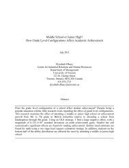
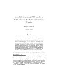
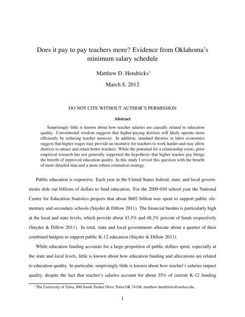
differenced equation, I use the district’s mandated salary increase required to meet the minimumsalary schedule as an instrument for a district’s change in salary schedule. This method producesa consistent estimator for the causal relationship between teacher salaries and student outcomesas long as the state’s minimum salary schedule is sufficiently correlated with teacher pay and thestate’s minimum salary schedule is uncorrelated with district-level time-varying unobservables thatinfluence student achievement and teacher outcomes.The Oklahoma state minimum teacher salary schedule was first established as part of HouseBill 1017 2 and first took effect during the 1991-92 school year. The state minimum salary schedulewas adjusted twice during the period for which data on teacher pay and student achievementare available. Between the 2005-06 and 2006-07 school years Oklahoma increased its minimumteacher salary schedule by $3,000 for every teacher. In the following year, the schedule was againincreased, but this time the raises varied by teacher experience and degree. The 2007-08 minimumsalary schedule included a raise of $600 for all teachers with under 10 years of experience. Forteachers with 10 or more years of experience the raises in the minimum salary schedule dependedon education: $1,025 for teacher with a Bachelor’s degree; $1,450 for teachers with a Master’s degree;$2,300 for teachers with a Doctoral degree. Oklahoma has not changed the minimum salaryschedule since 2008.Figure 1 illustrates the average (across years of experience) state minimum salary schedule forteachers who have a Bachelor’s degree and varying years of experience over the time period 2005-06 through 2011-12. Notice the large increase in the minimum salary schedule in 2006-07 for allexperience levels and the smaller increase in the salary schedule in 2007-08.A key requirement for the 2SLS estimation is that the state minimum salary schedule musthave an influence on teachers’ actual salaries. In other words, the minimum salary schedule mustbe binding for some districts. Figure 2 provides illustrative evidence that this is indeed the case.Figure 2 shows the mean contract salary paid to teachers with a Bachelor’s degree and 0-9 yearsof experience for each of the 39 districts in the sample. For each district, the changes in the state2 Laws 1989, 1st Ex. Session, c.29

Figure 1: State Minimum Salary Schedule by YearSalary in thousands30 35 402006 2008 2010 2012Yearmin BA salary 0-4yrsmin BA salary 10-14yrsmin BA salary 5-9yrsmin BA salary 15-25yrsFigure 2: District Average Contract Salaries for BA 0-9yrs by YearSalary in thousands30 32 34 36 382006 2007 2008 2009 2010 2011 2012Yearnumber of districts = 3910

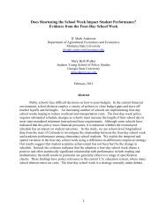
minimum salary schedule are closely matched by changes in the districts’ salary schedules.Figure 2 also identifies a potential weakness of the data. In order to separate the effect of achange in the district salary from a year effect, there must be sufficient variation in the timing ofdistrict salary changes. Ideally, within each year there would be a group of districts that changedtheir salary schedule (a treatment group) and a group of district that did not alter their salaryschedule (a control group). This type of variation would allow one to clearly separate the effectof a change in wage on the outcome variable from a year effect. As the figure illustrates, and aslater results show, there is not significant variation in the timing of salary changes across districts,which makes the separate identification of year fixed-effects and salary effects difficult.4 Results4.1 Turnover analysisI begin the analysis by probing for an indirect link between teacher pay and education qualityby examining the relationship between salaries and teacher turnover. Figure 3 illustrates changesin the median teacher turnover rate and median teacher pay for the largest 39 districts in Oklahomaover the years 2006-2012. Although the data provides a limited view of the long-term trends, thereappears to be a negative relationship between teacher turnover and teacher salaries. For example,from 2006 to 2010 median teacher salaries increased by about 10 percent, and at the same timeover this period the median turnover rate decreased by 5 percentage points, which is nearly a 40percent decline in the median turnover rate.To formally test for a relationship between teacher pay and turnover, tables 1 and 2 presentfirst-difference (FD), fixed-effects (FE), and first-difference by two-stage least squares (FD 2SLS)estimates of equation 1. For each table, I estimate equation 1 using a measure of voluntary teacherturnover as the dependent variable, which is defined as follows:V olT urn jt = #leavers jt − #cut jt#teachers jt(2)11

Figure 3: Median Salaries and Median Turnover by YearSalary in thousands30 31 32 33 34 358 10 12 14% Teacher Turnover2006 2008 2010 2012YearMedian BA salary 0-9yrsMedian Voluntary Turnover %Min Salary Sched. BA 0-9yrswhere V olT urn jt is voluntary turnover in district j at time t, #leavers jt is the number of teacherswho were in district j during time t but were not employed in district j during time t + 1,#teachers jt is the number of teachers in district j during time t, and #cut jt is the number ofteaching positions cut: #teachers jt -#teachers j,t+1 if the difference is greater than or equal tozero.In all specifications I control for county level economic conditions with measures of the averageearnings of workers in the service sector and unemployment rates. In addition to these controlvariables, the tables show estimates of three separate specifications, which are reported by column.In columns 1 and 4 of table 1 and column 1 of table 2, I report estimates of equation 1 by controllingfor district fixed-effects and assuming year fixed-effects are zero. In columns 2 and 5 of table 1and column 2 of table 2, I control for state-level effects by adding a time trend. In columns 3 and6 of table 1 and column 3 of table 2, I drop the time trend and control for state-level effects withyear fixed-effects.In both tables the key explanatory variable used to measure the district’s salary schedule is thedistrict’s mean contract salary for teachers with a Bachelor’s degree and 0-9 years of experience.12

The average salary was calculated using the district’s contract salary, not observed teacher salaries.For example, this was constructed by averaging the contract salaries for each of the following10 cells on the district’s salary schedule: BA and 0 years experience through BA and 9 years ofexperience. In both tables I estimate the effect of teacher salaries on the next period’s voluntaryteacher turnover (the effect of teacher salary in period t on turnover in period t + 1). In table1, columns 1-3 differ from columns 4-6 in estimation method. I report FD estimation results incolumns 1-3 and FE results in columns 4-6.Table 1: First Differencing and Fixed EffectsDependent Var: (1) (2) (3) (4) (5) (6)Voluntary Turnover t+1 FD FD FD FE FE FEBA salary 0-9yrs/1,000 -0.973*** -1.108*** -0.405 -0.960*** -1.071*** -0.454*(0.264) (0.298) (0.363) (0.263) (0.286) (0.256)Avg Earn in County/1,000 1.085*** 0.562 0.249 0.711** 0.551 0.307(0.286) (0.529) (0.348) (0.320) (0.451) (0.330)County Unemp. Rate -1.134*** -1.470*** -0.885 -0.745*** -0.943*** -0.057(0.194) (0.322) (0.593) (0.171) (0.291) (0.580)Observations 156 156 156 195 195 195R 2 0.188 0.204 0.357 0.205 0.208 0.353District FEs Yes Yes Yes Yes Yes YesTime Trend No Yes No No Yes NoYear FEs No No Yes No No YesNumber of Districts 39 39 39 39 39 39standard errors in parenthesesstandard errors are robust to arbitrary heteroskedasticity and correlation within districtdependent variable is percent voluntary turnover in t+1*** p

is zero (i.e. the minimum salary schedule was non-binding).Appendix table 4 shows first stage results for the 2SLS estimates in table 2. Notice the instrumentis strongly related to district salary when controlling for county economic conditions anddistrict fixed effects and a time trend, but not significant when controlling for year fixed-effects. Asa result, the FD 2SLS estimate in column 3 of table 2 should be disregarded since the instrumentalvariable is invalid in that specification.Table 2: First Differencing by 2SLSDependent Var: (1) (2) (3)Voluntary Turnover t+1 FD 2SLS FD 2SLS FD 2SLSBA salary 0-9yrs/1,000 -1.287*** -1.424*** -12.258(0.332) (0.370) (12.044)Avg Earnings in County/1,000 1.367*** 0.729 0.997(0.314) (0.471) (1.485)County Unemp. Rate -1.170*** -1.565*** -0.790(0.196) (0.323) (1.372)Observations 156 156 156District FEs Yes Yes YesTime Trend No Yes NoYear FEs No No Yesstandard errors in parenthesesstandard errors are robust to arbitrary heteroskedasticity and correlation within districtdependent variable is percent voluntary turnover in t+1district’s mandated salary increase for min salary compliance used as instrument*** p

this complication, the FE model still suggests a negative and statistically significant relationshipbetween teacher salary and turnover.The models also indicate other effects that are consistent with economic theory. In additionto the effects of teacher salaries on teacher turnover, the results suggests a positive relationshipbetween county-level earnings and teacher turnover. That is, as salaries in other occupations riserelative to teacher salaries, teacher turnover increases. Also, the models suggest a negative relationshipbetween county-level unemployment rates and teacher turnover. That is, as the probabilityof finding employment outside of teaching falls, fewer teachers will leave their current teachingposition. Both of these effects are consistent with what one would expect if teachers are responsiveto alternative employment opportunities.The size of the estimated effects in these models is fairly substantial. For example, as a conservativecalculation, if one accepts the smallest of the estimated effects presented above (-0.5) asthe true causal effect of teacher salary on turnover, then that suggests a $2,000 increase in teachersalary will reduce a district’s voluntary turnover rate by one percentage point. While that soundssmall, in Oklahoma the average district voluntary turnover rate in 2011 was 12 percent, or 12 outof 100 teachers turnover each year. Therefore a $2,000 increase in teacher pay would reduce this to11 percent, which is an 8 percent reduction in the turnover rate. The higher end estimates suggestthat a $2,000 increase in teacher pay would reduce teacher turnover by as much as 2 percentagepoints, which is roughly a 17 percent reduction in the turnover rate.4.2 Characteristics of new teacher hiresanalysis forthcoming4.3 Student test scoresanalysis forthcoming15

4.4 Dropout ratesanalysis forthcoming5 ImplicationsforthcomingReferencesAkerlof, George A. 1982. “Labor Contracts as Partial Gift Exchange.” The Quarterly Journal ofEconomics, 97(4): 543–569.Clotfelter, Charles, Elizabeth Glennie, Helen Ladd, and Jacob Vigdor. 2008. “Would HigherSalaries Keep Teachers In High-poverty Schools? Evidence from a Policy Intervention inNorth Carolina.” Journal of Public Economics, 92(56): 1352–1370.Hanushek, Eric A., and Steven G. Rivkin. 2010. “Generalizations about Using Value-AddedMeasures of Teacher Quality.” American Economic Review, 100(2): 267–271.Hanushek, Eric A., John F. Kain, and Steven G. Rivkin. 2004. “Why Public Schools LoseTeachers.” The Journal of Human Resources, 39(2): pp. 326–354.Hanushek, Eric A., John F. Kain, Daniel M. O’Brien, and Steven G. Rivkin. 2005. “TheMarket for Teacher Quality.” National Bureau of Economic Research Working Paper 11154.Hanushek, Eric A., Steven G. Rivkin, Richard Rothstein, and Michael Podgursky. 2004.“How to Improve the Supply of High-Quality Teachers.” Brookings Papers on EducationPolicy, , (7): 7–44.Heckman, James J., and Bo E. Honor. 1990. “The Empirical Content of the Roy Model.” Econometrica,58(5): pp. 1121–1149.Jacob, Brian A., and Lars Lefgren. 2008. “Can Principals Identify Effective Teachers? Evidenceon Subjective Performance Evaluation in Education.” Journal of Labor Economics,26(1): 101–136.Kane, Thomas J., and Douglas O. Staiger. 2008. “Estimating Teacher Impacts on StudentAchievement: An Experimental Evaluation.” National Bureau of Economic Research WorkingPaper 14607.Kane, Thomas J., Jonah E. Rockoff, and Douglas O. Staiger. 2008. “What Does CertificationTell Us About Teacher Effectiveness? Evidence from New York City.” Economics of EducationReview, 27(6): 615–631.16

Loeb, Susanna, and Marianne E. Page. 2000. “Examining the Link between Teacher Wages andStudent Outcomes: The Importance of Alternative Labor Market Opportunities and Non-Pecuniary Variation.” The Review of Economics and Statistics, 82(3): 393–408.Rockoff, Jonah E. 2004. “The Impact of Individual Teachers on Student Achievement: Evidencefrom Panel Data.” The American Economic Review, 94(2): 247–252.Ronfeldt, Matthew, Hamilton Lankford, Susanna Loeb, and James Wyckoff. 2011. “HowTeacher Turnover Harms Student Achievement.” National Bureau of Economic ResearchWorking Paper 17176.Rothstein, Jesse. 2010. “Teacher Quality in Educational Production: Tracking, Decay, and StudentAchievement.” Quarterly Journal of Economics, 125(1): 175–214.Roy, A. D. 1951. “Some Thoughts on the Distribution of Earnings.” Oxford Economic Papers,3(2): pp. 135–146.Shapiro, Carl, and Joseph E. Stiglitz. 1984. “Equilibrium Unemployment as a Worker DisciplineDevice.” The American Economic Review, 74(3): 433–444.Snyder, T. D., and S. A. Dillow. 2011. Digest of Education Statistics 2010 (NCES 2011-015).National Center for Education Statistics, Institute of Education Sciences, U.S. Department ofEducaton. Washington, DC.Staiger, Douglas O., and Jonah E. Rockoff. 2010. “Searching for Effective Teachers with ImperfectInformation.” Journal of Economic Perspectives, 24(3): 97–118.AAppendix17

Table 3: Districts in Sample: Characteristics in 2009-10District Students FTE TeachersALTUS 4,001 280.5ARDMORE 3,081 205.8BARTLESVILLE 5,971 400.5BIXBY 4,784 267.8BROKEN ARROW 16,618 952.5CLAREMORE 4,168 270COWETA 3,263 194DEER CREEK 3,577 229.9EDMOND 20,750 1,174.80EL RENO 2,453 163.8ENID 6,896 450.7GROVE 2,561 163.1GUTHRIE 3,309 216.4GUYMON 2,726 167.1HARRAH 2,235 153.1JENKS 10,162 577.6LAWTON 16,398 1,117.80MIDWEST CITY-DEL CITY 14,643 947.5MOORE 21,675 1,285.50MUSKOGEE 6,567 383.4MUSTANG 8,607 503.8NORMAN 14,363 943.2OKLAHOMA CITY 42,549 2,589.60OWASSO 9,034 497.9PONCA CITY 5,157 330.2PUTNAM CITY 18,700 1,199.60SAND SPRINGS 5,412 327.3SAPULPA 4,149 253.6SHAWNEE 4,120 262.3SKIATOOK 2,546 144.2STILLWATER 5,650 360TAHLEQUAH 3,555 243.7TECUMSEH 2,299 155TULSA 41,493 2,739.00UNION 15,010 865.7WAGONER 2,475 179.1WESTERN HEIGHTS 3,534 254.4WOODWARD 2,684 161.5YUKON 7,209 414.839 District Total 354,384 22,027STATE TOTAL 654,802 42,614Percent of State Total 54% 52%18

Table 4: 2SLS First Stage ResultsDependent Var: (1) (2) (3)change in BA salary 0-9yrs OLS OLS OLSState Mandated Salary Increase 1.268*** 1.221*** 0.091(0.135) (0.118) (0.078)Observations 156 156 156R 2 0.754 0.766 0.917District FEs Yes Yes YesTime Trend No Yes NoYear FEs No No Yescluster-robust standard errors in parentheses*** p