Analytical solution of Burgers-like equation - Ultrascientist.org

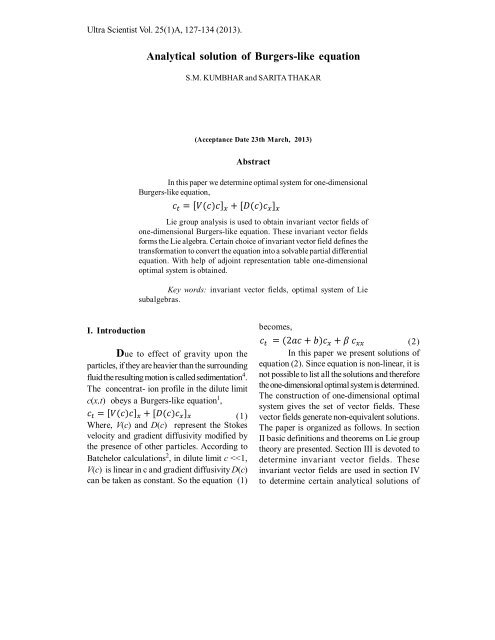
Ultra Scientist Vol. 25(1)A, 127-134 (2013). 

Analytical solution of Burgers-like equation 

S.M. KUMBHAR and SARITA THAKAR 

(Acceptance Date 23th March, 2013) 

Abstract 

In this paper we determine optimal system for one-dimensional 

Burgers-like equation, 

Lie group analysis is used to obtain invariant vector fields of 

one-dimensional Burgers-like equation. These invariant vector fields 

forms the Lie algebra. Certain choice of invariant vector field defines the 

transformation to convert the equation into a solvable partial differential 

equation. With help of adjoint representation table one-dimensional 

optimal system is obtained. 

Key words: invariant vector fields, optimal system of Lie 

subalgebras. 

I. Introduction 

Due to effect of gravity upon the 

particles, if they are heavier than the surrounding 

fluid the resulting motion is called sedimentation 4 . 

The concentrat- ion profile in the dilute limit 

c(x,t) obeys a Burgers-like equation 1 , 

(1) 

Where, V(c) and D(c) represent the Stokes 

velocity and gradient diffusivity modified by 

the presence of other particles. According to 

Batchelor calculations 2 , in dilute limit c

128 S.M. Kumbhar, et al. 

equation (2). In section V, adjoint representation 

table is constructed and is used to determine 

one-dimensional optimal system. Conclusions 

are given at the end. 

II. Preliminaries: 

In this section we state the basic 

definitions and theorems on symmetry group 

and Lie algebra 3 . 

i) The General Prolongation formula: Let 

ii) Theorem 1: Suppose 

, , 

is a system of differential equations of maximal 

rank defined over 

. If G is a local 

group of transformations acting on M, and 

, whenever , 

for every infinitesimal generator of G, then 

G is a symmetry group of the system. 

III. Invariant vector fields: 

be a vector field defined on an open subset 

MX U. The n th prolongation of is the vector 

field 

(3) 

In this section we determine invariant 

vector fields for equation (2). On applying 

theorem 1 and general prolongation formula 

(3), we determine the symmetry group of 

equation (2). Suppose the symmetry group of 

equation (2) is generated by vector field, 

defined on the corresponding jet space 

, the second summation being 

over all multi-indices , 

with , . The coefficient 

functions of are given by the 

formula: 

On applying the second prolongation of vector 

field on equation (2) we get, 

where, 

where, and .

Analytical solution of Burgers-like equation. 129 

The generators are functions 

of t, x, c and are independent of partial 

derivatives of c with respect to t and x. On 

substituting the expression for 

in 

equation (5) and on equating the coefficients 

of equal powers of partial derivatives of c w.r.t. 

x and t we get the following system of 

equations. 

The commutation relations between 

vector fields are given by the following table 1. 

The entry in row i and column j representing 

and is defined as 

On simultaneous evaluation of above system 

of equations we get, 

. 

. 

Table 1. Commutator table for 5 parameter 

Lie algebra 

1 2 3 4 5 

1 0 0 2 1 2 1 

2 0 0 0 3 

3 2 0 0 3 0 

4 1 2 3 0 5 

where 

. 

are arbitrary constants. 

With respect to each constant C i we get an 

invariant vector field. Thus the Lie algebra is 

generated by the following five vector fields. 

5 4 3 0 5 0 

Since the set of invariant vector fields 

forms a linear space any linear combination 

of these vectors is also an invariant vector 

field. In section IV we determine solutions of 

equation (2) by using invariant vector fields 

5 and 1 + 5 .


IV. Analytical solution: 

In this section we determine some 

solutions of equation (2). To determine the 

analytic solution of equation (2) vector field 5 

is used to define new independent and 

dependent variables. Correspond to vector 

field 5 we get the characteristic equation 

We define new independent variables as 

(9) 

(10) 

this leads to a system of ordinary differential 

equations, 

and 

From above characteristic equation define new 

variables , and 

In the phase plane we get 

We treat µ as new 

dependent variable. Since, and θ are functions 

of x and t we treat and θ as new independent 

variables. With this choice of new variables 

equation (2) becomes, 

(6) 

Equation (6) is a standard onedimensional 

Burgers equation. Here, we use 

First integral method 1 to find analytical solution 

of equation (6). We use transformation 

By integrating above equation, we get 

where k 1 is integrating constant. 

On integrating above differential equation, we 

get 

where k 2 is integrating constant and 

, where (7) 

Then by using chain rule, 

But 

X = µ and 

(8) 

therefore, we have 

With the representation given in equation (7) 

equation (6) gets converted in to an ordinary 

differential equation 

(11)


which is analytical solution of equation (2). 

The solution (11) obtained from vector 

field 5 is defined for t > 0. Non-singular solution 

of equation (2) is obtained from vector field 

1 + 5 . The characteristic equation corresponding 

to the vector field 1 + 5 is 

From the above characteristic equation define 

new independent variables and as = tan -1 

On equating the coefficients of equal powers 

of we get k() and k 1 () as follows 

and 

Where, c 1 and c 2 are constants of integration. 

Thus from equation (13) we get 

t and 

. And the new dependent 

Since 

we have 

variable denoted by µ is defined as 

with this choice of new variables, equation (2) 

becomes 

(15) 

Another solution of equation (12) can be obtained 

by assuming that 

(16) 

Since equation (16) is solution of equation (12), 

we get 

Equation (12) is purely non-linear and different 

functional forms will provides different 

solutions to equation (12). In this section we 

report two different solutions. 

Suppose, 

then (13) 

Since , equation (12) 

becomes 

From equation (13) and (14) we get, 

(14) 

On equating the coefficients of equal powers 

of we get and as follows 

and 

where c 3 

is constant of integration. 

Thus from equation (16) we get 

Since 

we have


V. One dimensional optimal system: 

In section IV we have seen that there 

are many solutions available for equation (2) 

and it necessary to classify all solutions into 

different categories. This classification is achieved 

by constructing one dimensional optimal 

system. The problem of finding an optimal 

system of subgroups is equivalent to that of 

finding an optimal system of subalgebras. For 

one-dimensional subalgebra this classification 

is essentially the same as the problem of 

classifying the orbits of the adjoint representation. 

From the commutator table we obtain the 

adjoint representation table 2. To compute 

adjoint representation we use the Lie series 

For finding one-dimensional optimal system, 

we consider 

Suppose without loss of generality let 

. If we act on such a by , 

then we can make the coefficient of v 3 vanish 

and we get 

The coefficients 

are 

functions of 

. Next we act on v' 

by 

of v 4 , leading to 

to cancel the coefficient 

Table 2. Adjoint representation of Lie 

subalgebra of dimension 5 

Ad 1 2 3 4 5 

1 1 2 3 4 5 

2 1 4 

1 

2 1 2 3 4 5 

For certain depending on . 

Next we act on v" by 

to 

eliminate the coefficient v 2 , leading to 

3 

3 1 2 3 4 + 5 

2 3 

4 1 4 

5 1 + 2 3 4 

4 + 3 5 5 

5 

For certain depending on . we can 

further act on v'" by 

. This has 

the net effect of scaling the coefficients of v 1 

and v 5 

We can make the coefficient of v 1 either or 

+1,1 or 0. Then one-dimensional subalgebras


spanned by a general vector field v with a 5 0 

is equivalent to an algebra spanned by {v 1 +v 5 , 

v 1 + v 1 + v 5, + v 5 }. 

The remaining one-dimensional 

subalgebras are spanned by vectors of the 

form 

If we act on such a v by Ad (exp (a 1 v 1 )), we 

can make the coefficient of v 1 vanish and we 

get 

For certain 

we act on v' by 

the coefficient v 2 , leading to 

depending on a 1 ,a 2 ,a 3 . Next 

to cancel 

further act on v' by 

. this 

operation has the net effect of scaling the 

coefficients of v 1 and v 3 

We can make the coefficient of v 1 

either +1,1 or 0. Then one-dimensional 

subalgebras generated by v with a 5 =a 4 =0, a 3 0 

is equivalent to an algebra spanned by {v 1 +v 3, 

v 1 +v 3, v 3 

The remaining one-dimensional 

subalgebras are spanned by vectors of the 

above form with a 5 =a 4 =a 3 0, a 2 0 and a 2 =1, 

v becomes, 

For certain depending on . Next 

If we act on such a v by 

we act on v" by 

cancel the coefficient v 3 , leading to 

to 

then the coefficient of v 2 vanish: 

Every one-dimensional subalgebra generated 

by v with 

algebra spanned by {v 4 }. 

is equivalent to the 

Similarly with anda 3 =1, 

we get 

Every one-dimensional subalgebra 

generated by v with a 5 =a 4 =a 3 0, a 2 0 is 

equivalent to the algebra spanned by {v 1 }. 

Thus the optimal system of onedimensional 

subalgebras are spanned by 

If we act on such a v by , 

we can make the coefficient of v 2 vanish 

For certain depending on We can

134 Ultra Scientist Vol.25(1)A, (2013). 

invariant in time as well as in space coordinates. 

A singular solution of equation (2) 

is obtained from vector field. Two solutions 

are obtained by using a linear combination of 

two vector fields and first integral method. 

Optimal system consisting of eight onedimensional 

subalgebras is obtained. The 

generators of there subalgebras are listed at 

the end. 

References 

Conclusion 

The symmetry algebra of Burger-like 

equation (2) is spanned by five vector fields. 

The solutions of equation (2) are translation 

1. A.J.S. Al-Saif and Ammar Abdul-Hussein, 

Generating exact solutions of two 

dimensional coupled Burgers equations 

by the first integral method, Research 

Journal of physical and applied science 

Vol. 1(2), pp 029-033, (November 2012). 

2. L. V. Ovsiannikov, Group Analysis of 

Differential Equations, Academic Press, 

(1982). 

3. P. J. Olver, Applications of Lie groups to 

differential equations, Springer–Verlag, 

New York (1986). 

4. Sergei E. Esipov, Coupled Burgers 

equations: A model of polydispersive 

sedimentation, Physical review E, Volume 

52, Number 4, (Octomber 1995).

Analytical solution of Burgers-like equation - Ultrascientist.org

You also want an ePaper? Increase the reach of your titles

Delete template?

Save as template?