s - Athanasios Dermanis Home Page
s - Athanasios Dermanis Home Page
s - Athanasios Dermanis Home Page
Create successful ePaper yourself
Turn your PDF publications into a flip-book with our unique Google optimized e-Paper software.
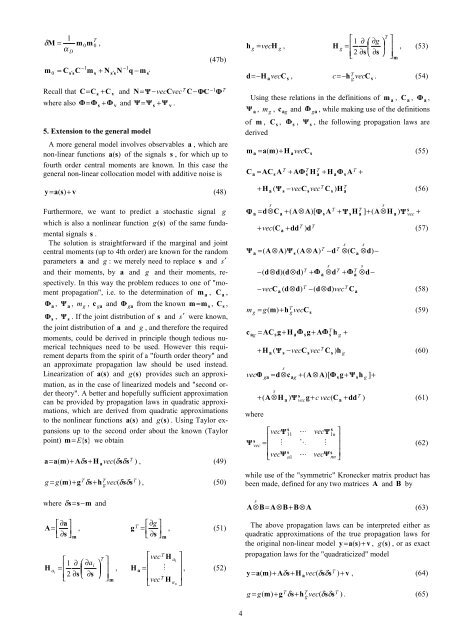
1 T<br />
δ M = m 0m<br />
0 , α<br />
D<br />
−1<br />
−1<br />
m 0 = Cs′ sC<br />
m s + N s′<br />
sN<br />
q − m s′<br />
-&<br />
(47b)<br />
Recall that C = C s + C v and N=<br />
−vecCvec T C−<br />
−1-T<br />
where also - = - s + - v and = s + v .<br />
5. Extension to the general model<br />
A more general model involves observables a , which are<br />
non-linear functions a (s)<br />
of the signals s , for which up to<br />
fourth order central moments are known. In this case the<br />
general non-linear collocation model with additive noise is<br />
y = a( s)<br />
+ v<br />
(48)<br />
Furthermore, we want to predict a stochastic signal g<br />
which is also a nonlinear function g (s)<br />
of the same fundamental<br />
signals s .<br />
The solution is straightforward if the marginal and joint<br />
central moments (up to 4th order) are known for the random<br />
parameters a and g : we merely need to replace s and s′<br />
and their moments, by a and g and their moments, respectively.<br />
In this way the problem reduces to one of "moment<br />
propagation", i.e. to the determination of m a , C a ,<br />
- a , a , m g , c g a and - g a from the known m= m s , C s ,<br />
- s , s . If the joint distribution of s and s′ were known,<br />
the joint distribution of a and g , and therefore the required<br />
moments, could be derived in principle though tedious numerical<br />
techniques need to be used. However this requirement<br />
departs from the spirit of a "fourth order theory" and<br />
an approximate propagation law should be used instead.<br />
Linearization of a (s)<br />
and g (s)<br />
provides such an approximation,<br />
as in the case of linearized models and "second order<br />
theory". A better and hopefully sufficient approximation<br />
can be provided by propagation laws in quadratic approximations,<br />
which are derived from quadratic approximations<br />
to the nonlinear functions a (s)<br />
and g (s)<br />
. Using Taylor expansions<br />
up to the second order about the known (Taylor<br />
point) m= E{s}<br />
we obtain<br />
a= a( m)<br />
+ Aδ s+<br />
H vec(<br />
s sT<br />
a δ δ ) , (49)<br />
g = g( m)<br />
+ gT<br />
δ s+<br />
h vec(<br />
δsδsT<br />
) , (50)<br />
where δ s=<br />
s−m<br />
and<br />
T g<br />
h g = vecH g ,<br />
H<br />
g<br />
⎡<br />
T<br />
1 ∂ ⎛ ∂g<br />
⎞ ⎤<br />
= ⎢ ⎜ ⎟ ⎥<br />
⎢2<br />
∂s<br />
s<br />
⎣ ⎝ ∂ ⎠ ⎥⎦<br />
m<br />
, (53)<br />
d= −H a vecC s , c= −h vecC s . (54)<br />
Using these relations in the definitions of m a , C a , - a ,<br />
a , m g , c ag<br />
and - g a , while making use of the definitions<br />
of m , C s , - s , s , the following propagation laws are<br />
derived<br />
m<br />
C<br />
a<br />
a<br />
= a( m)+<br />
H vecC<br />
(55)<br />
a<br />
= AC AT<br />
+ A-T<br />
H<br />
T<br />
+ H - AT<br />
+<br />
s<br />
s<br />
s<br />
a<br />
a<br />
+ H ( −vecC<br />
vec T C ) H<br />
(56)<br />
a<br />
s<br />
s<br />
s<br />
s<br />
- = ⊗ + ⊗ + + ⊗<br />
s<br />
a d Ca<br />
( A A)[<br />
-s<br />
AT<br />
sH<br />
T<br />
a ] ( A H a ) vec<br />
a<br />
m<br />
c<br />
s<br />
s<br />
T<br />
a<br />
+ vec( +<br />
T T<br />
(57)<br />
C a dd ) d<br />
= ( A⊗A)<br />
( A⊗A)<br />
T<br />
−dT<br />
⊗(<br />
C ⊗d)<br />
−<br />
−(<br />
d⊗d)(<br />
d⊗d<br />
s<br />
) T<br />
+ -<br />
a<br />
s<br />
⊗d<br />
T<br />
s<br />
T g<br />
+ -<br />
a<br />
s<br />
s<br />
T<br />
a<br />
T<br />
T<br />
a C a<br />
⊗d−<br />
− vec C ( d⊗d)<br />
−(<br />
d⊗d)<br />
vec<br />
(58)<br />
= g( m)<br />
h vec<br />
(59)<br />
g +<br />
ag<br />
vec<br />
where<br />
<br />
s<br />
vec<br />
T g<br />
C s<br />
= AC + +<br />
T<br />
sg<br />
H a-<br />
sg<br />
A-s<br />
h g +<br />
+ H ( −vecC<br />
vec T C h<br />
(60)<br />
a s s s )<br />
s<br />
- ga<br />
ag<br />
( s s g<br />
= d⊗c<br />
+ A⊗A)[<br />
- g+<br />
h ] +<br />
s<br />
g<br />
+ ( A⊗H<br />
) <br />
s<br />
g+<br />
c vec(<br />
C ddT<br />
)<br />
(61)<br />
⎡vec<br />
⎢<br />
= ⎢ <br />
⎢<br />
⎣vec<br />
a vec<br />
a +<br />
s<br />
11<br />
s<br />
n1<br />
<br />
<br />
<br />
vec<br />
<br />
vec<br />
s<br />
1<br />
n<br />
<br />
s<br />
nn<br />
⎤<br />
⎥<br />
⎥<br />
⎥<br />
⎦<br />
+<br />
(62)<br />
while use of the "symmetric" Kronecker matrix product has<br />
been made, defined for any two matrices A and B by<br />
A⊗ s B=<br />
A⊗B+<br />
B⊗A<br />
(63)<br />
⎡∂a<br />
⎤<br />
A= ⎢<br />
s<br />
⎥ ,<br />
⎣ ∂ ⎦<br />
H<br />
m<br />
⎡1<br />
∂ ⎛ ∂ai<br />
⎞<br />
= ⎢ ⎜ ⎟<br />
⎢ ∂s<br />
s<br />
⎣ ⎝ ∂ ⎠<br />
ai 2<br />
T<br />
⎤<br />
⎥<br />
⎥<br />
⎦<br />
m<br />
,<br />
g<br />
T ⎡∂g<br />
⎤<br />
= ⎢<br />
s<br />
⎥<br />
⎣ ∂<br />
, (51)<br />
⎦<br />
H a<br />
m<br />
⎡vecT<br />
H<br />
⎢<br />
= ⎢ <br />
⎢ T<br />
⎣<br />
vec H<br />
a1<br />
a n<br />
⎤<br />
⎥<br />
⎥ , (52)<br />
⎥<br />
⎦<br />
The above propagation laws can be interpreted either as<br />
quadratic approximations of the true propagation laws for<br />
the original non-linear model y = a( s)<br />
+ v , g (s), or as exact<br />
propagation laws for the "quadraticized" model<br />
y = a( m)<br />
+ Aδ s+<br />
H a vec(<br />
δsδsT<br />
) + v , (64)<br />
g = g( m)<br />
+ gT<br />
δ s+<br />
h vec(<br />
δsδsT<br />
) . (65)<br />
T g<br />
4


