geometric correction

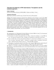
Chapter 4Image registration(geometric correction)Particular types of image transformations are those where the “appearance”of the image is preserved and only its geometric form is altered.The process of the transformation is called geometric correction and theresult as image registration. The purpose of such a transformation is tomatch the form of either another image (image-to-image registration) ora map of the same area in a particular cartographic projection (image-tomapregistration).4.1. Geometric image transformationLet i , j are the row and column numbers of a particular pixel (fig. 4.1),x , y the coordinates of the center of the pixel on the map and λ , φ itsspherical (geographic) coordinates on the earth surface. A rigorousmathematical solution to the registration problem should involve the“projective transformation”( i , j)= χ(λ,φ)(1)from the spherical surface of the earth to the existing image, its inverse−1( λ , φ)= χ ( i,j), (2)Figure 4-1as well as the particular cartographic projection transformation( x , y)= ψ ( λ,φ). (3)

CHAPTER 4A. DERMANIS: REMOTE SENSINGFigure 4-2: The image to map transformationThe image-to-map registration (fig. 4.2) would be realized in this case bythe combined transformations( x,y)= χ−1−1ψ ( ( i,j)), ( i,j)= ( ψ ( x,y))χ . (4)If the projective transformations for two images a and b are( i a , j a ) = χ a ( λ,φ)and ( i b , j b ) = χ b ( λ,φ)respectively, the image-toimageregistration would be realized by the combined transformations( i , jbb−1−1χ ( ( i , j )), ( i , j ) = ( χ ( i , j ))) = χbaaaaaχ . (5)We shall restrict from know on the discussion to the image-to-map registrationproblem, bearing in mind that the treatment of the image-to-imageregistration is completely analogous.Between the two transformations in (4) the one we need is in fact thesecond, i.e. the map-to-image transformation (fig. 4.3). Indeed our purposeis not to find where the image pixels are located on the map, butrather where the pixels of a “digitized” map are located on the image. Inthis way values for the map pixels can be assigned on the basis of thevalues of the image pixels and the digital map can be realized in the formof a new digital file, the “registered to the map” image.−1In our search for the transformation ( i,j)= χ ( ψ ( x,y)) the cartographicprojection transformation ψ is always well defined, since it is a matterof choice from a set of available such mathematical transformations. Thisis not the case however for the image projective transformation χ ; it dependson the sensor position and orientation, it is affected by their temporalvariation during the time interval required for the observation ofthe image and furthermore involves the heights h of points, i.e., it hasthe form ( i,j)= χ(λ,φ,h). For this reason a simpler “empirical” approachis followed. The unknown transformationabbb−1χ ψ is replaced by2

Image registration (geometric correction)some model function f depending on a number of unknown parameters.Figure 4-3: The map-to-image transformationThese parameters are determined from the measured or known coordinatesfor a number of points in both the original image and the final image(map or second image). Thus the transformation for image-to-mapregistration has the form( 1 2pi,j)= f ( x,y,p , p , , ps ) = f ( x,x,) , (6)where the parameters p = [ p 1,p2,,p s ] are to be estimated with thehelp of the observed coordinates ( i k , jk) and ( x k , yk) , k = 1,2,,n of npoints, which are easily identifiable on both image and map. The estimationof the transformation parameters p follows from the solution of thesystem of 2 n equations (2 for each point)i , j ) = f ( x , y , p , p , ,p ) ,( 1 1 1 1 1 2 s( i , j2)= f ( x2,y2,p1,p2,,p ) ,2 s( i , j ) = f ( x , y , p , p2,,p ) . (7)nnnn1 sIn general 2 n > s is chosen and the resulting inconsistent system withmore equations than unknowns, is approximately solved using a leastsquares method, where the sum of the squares of the residuals (differencesbetween left and right sides) is minimized in order to obtain optimalvalues of the parameters p . The whole procedure is greatly facilitatedif the model ( i , j)= f ( x,y,p)is linear with respect to the parame-T3

CHAPTER 4A. DERMANIS: REMOTE SENSINGnT2 2v v = ∑(vx+ vy) = min(15)k kk = 1is well known to be given by the unique solution of the normal equationsTT( A A)ˆz = A b , which explicitly is−− ⎡aˆTTT 1 TT 1 T ⎤ ⎡QQ 0 ⎤ ⎡Qi⎤⎡(Q Q)Q i⎤zˆ = ( A A)A b = ⎢ ⎥ = ⎢ ⎥ ⎢ ⎥ = ⎢ − ⎥⎣bˆ. (16)TTT 1 T⎦ ⎣ 0 Q Q⎦⎣Qj⎦⎣(Q Q)Q j⎦The corresponding individual residualsvˆ= b − Azˆ, (17)as well as the single collective parametervˆT vˆσ ˆ 2 = , (18)fgive a measure of the “accuracy” with which the model has been fitted tothe known points. The integer f = 2 n − s , called the degrees of freedom,is the difference between the number of equations and the number of parameters.A value of σ ˆ significantly larger than 1, designates bad fit-2ting, in which case one or more points with large residuals should be removedand the solution should be repeated with the remaining points. Amore rigorous and more efficient treatment of the problem is givenwithin the framework of statistical estimation theory for the linear model(Gauss-Markov model), see e.g. Sansó (1996).As an example we give the solution for the linear transformation−1i i(x,y)= a + a x + a y = ti + a x + b y= 00 10 01j j(x,y)= b + b x + b y = t j + c x + d y= 00 10 01(19)The solution is obtained after performing all the above matrix calculationsand has the form2ysxi2 2sxsys − s s s ρi xi − ρ ρ yiaˆ= =, (20)− s 1−ρxy yi2sxyxxy2xy2ysxj2 2sxsys − s s s j ρ xj − ρ ρ yjcˆ= =, (21)− s 1−ρxy yj2sxyxxy2xy6

Image registration (geometric correction)2xsyi2 2sxsyˆs − s s s ρi yi − ρ ρ xib = =, (22)− s 1 − ρxy xi2sxyyxy2xy2xsyj2 2sxsyˆs − s s s j ρ yj − ρ ρ xjd = =, (23)− s 1−ρxy xj2sxyyxy2xytˆi= m − aˆm − bˆm , (24)ixytˆj= m − cˆm − dˆm , (25)jxyˆvik= i − tˆ− aˆx − bˆy , (26)kikkˆv j k= j − tˆ− cˆx − dˆy , (27)kjkkwhere the means mx, m y , m i , m j , the variances s 2 x ,standard deviations s x , s y , s i , s j , the covariances s xyand the correlationsmm1=n∑x x kk1=n∑y y kk2s y ,2s i ,2s j , the, s xi , s xj , s yi , syjρ xy , ρ xi , ρ xj , ρ yi , ρ yj are computed as follows:, (28), (29)1m =n∑i i kk, (30)m1=n∑j j kk, (31)s2x12 2= ∑ ( xk− mx)≡ ( sx), (32)nks2y12 2= ∑ ( yk− my) ≡ ( sy) , (33)nk7

CHAPTER 4A. DERMANIS: REMOTE SENSING2is12 2= ∑ ( ik− mi) ≡ ( si) , (34)nks2j12 2= ∑ ( jk− m j ) ≡ ( s j ) , (35)nksxy1= ∑ ( xk− mx)(yk− my) ≡ sxsyρnkxy, (36)sxi1= ∑ ( xk− mx)(ik− mi) ≡ sxsiρxi, (37)nksyi1= ∑ ( yk− my)( ik− mi) ≡ sysiρyink(38)sxj1= ∑ ( xk− mx)(jk− m j ) ≡ sxsjρxj , (39)nksyj1= ∑ ( yk− my)( jk− m j ) ≡ sysjρyj. (40)nkFor the rotation-scaling-translation model⎡i⎤ ⎡ a⎢ ⎥ = ⎢⎣ j⎦⎣−bb⎤⎡x⎤⎡ti⎤⎥⎢⎥ + ⎢ ⎥ , (41)a⎦⎣y⎦⎣t j ⎦a = s cosθ , b = ssinθ(42)the least squares solution is given bys + saˆ= , (43)s + sxi2xyj2yˆs − sb = , (44)s + syi2xxj2ytˆi= m − aˆm − bˆm , (45)ixytˆ= m + bˆm − aˆm(46)jjxy8

Image registration (geometric correction)ˆvik= i − aˆx − bˆy − tˆ, (47)kkkiˆv j k= j + bˆx − aˆy − tˆ, (48)kkkjb syi− sxjtanθ ˆ = ˆ= , (49)a ˆ s + sxiyj2 2 122sˆ= aˆ+ bˆ= ( sxi+ syj) + ( syi− sxj) . (50)s + s2x2y4.2. ResamplingFigure 4-4The transformation from the new image or map coordinates ( x,y)to theoriginal image pixel coordinates ( i , j), established as described in theprevious section, can be implemented in order to produce a new“registered” or “geometrically corrected” digital image, whichcorresponds to either the “target image” in image-to-image registration,or to the particular cartographic projection in image-to-map registration.The center of every map pixel has integer valued coordinates ( X , Y )which the established transformation i = i( x,y), j = j( X , Y ) maps (fig.4.4) into values I = i( X , Y ) , J = j( X , Y ) , which are not integer but realnumbers in general. We need therefore to evaluate values =V i( X , Y ). j(X , Y ) = VX. YV I . J= for all the map pixels or equivalently for all theresulting positions ( I,J ) on the original image, from the available valuesV i , j at the pixel centers ( i , j). This can be achieved with the help of aninterpolation of the available grid values V i , j , which is calledresampling.Figure 4-5: Closest neighbor interpolationThe simplest interpolation-resampling method is the method of the near-9

CHAPTER 4A. DERMANIS: REMOTE SENSINGest neighbor interpolation (fig. 4.5). If i ≤ I ≤ i + 1 and j ≤ J ≤ j + 1,i.e. the point ( I , J ) falls in the grid cell with vertices ( i , j), ( i , j + 1),( i + 1, j), ( i + 1, j + 1), the 4 distances from the vertices are evaluated22d i , j ( I − i)+ ( J − j)= , (51)22d , j + 1 = ( I − i)+ ( J − j −1)i , (52)221 , j = ( I − i −1)+ ( J − j)di+ , (53)22+ 1 , j + 1 = ( I − i −1)+ ( J − j −1)di , (54)the minimal one is determined, say d p , q and the value is set equal to thatof the nearest (neighboring) grid point V X , Y= VI, J= Vp,q .The nearest neighbor interpolation has the advantage that it assigns to thenew (registered) image pixel values that have been actually observed. Forthis reason it is the only reasonable method to use when image registrationis preceding image classification. In general image registrationshould follow classification, or other image transformations. Its disadvantageis that it produces images, which are not smooth with an obviouspixel-like effect, especially when the pixel size of the original image isdifferent from that of the new image. The pixel size of the new image isequal to that of the target image or map. The difference in pixel size canbe avoided in image-to-map registration by a proper choice of the mapscale. It is though unavoidable in image-to-image registration when thesensor of the original image is different from the sensor of the target image.The above problems of closest neighbor interpolation can be avoided byusing more appropriate interpolation methods, which produce smoothimages, such as the bilinear and the bicubical interpolation.Figure 4-6: The bilinear interpolationThe bilinear interpolation (fig. 4.6) is utilizing only the 4 grid values10

Image registration (geometric correction)around the interpolation point ( I , J ) and consists of a combination oftwo linear interpolations, one along the i axis and one along the j axis.In the first linear interpolation (along j ) the values of the upper gridpoints ( i , j), ( i , j + 1)are interpolated by a linear function, which producesat the point ( i , J ) the valueVi, J i,j ( i,j 1 i,j= V + J − j)(V + −V) . (55)In addition the values of the lower grid points ( i + 1, j)and ( i + 1, j + 1)are interpolated by a linear function, which produces at the point( i + 1, J ) the value= V + J − j)(V V ) . (56)V i+ 1,J i+1, j ( i+1, j + 1 −i+1,jIn the second interpolation (along i ) the produced values at the points( i,J ) and ( i + 1, J ) are linearly interpolated to produce the desired valueat ( I,J )V= V + I − i)(V + −V) . (57)I , J i,J ( i 1, J i,JThe resulting interpolated value becomesV= i + 1−I)(j + 1−J ) V , + ( J − j)(i + 1 − I V , +1 +I , J ( i j) i j+ ( − i)(j + 1−J ) Vi+ 1 , j+ ( I − i)(J − j)Vi+ 1, j+1I . (58)Figure 4-7: The bicubic interpolationNote that exactly the same interpolated value is obtained if the order of11

CHAPTER 4A. DERMANIS: REMOTE SENSINGthe linear interpolations is reversed: first along the i axis to produceV I , jand V I , j + 1 ; then along the j axis to produce V I , J .The bicubic interpolation (fig. 4.7) is utilizing 16 grid values around theinterpolation point and it consists of 4 cubic interpolations along the jaxis, followed by a cubic interpolation along the i axis. A cubic interpolationfits a third order polynomial with 4 unknown coefficients to 4points with known values. In the first step the 4 points in each of the 4rows are used to produce a value at the point on the same row with secondcoordinate J , according to the following scheme:V , V i 1,ji−1,j −1− , i−1 , j+1V , V , 2 → V i , Ji−1 j +−1V i, j −1 , i jV , , V 1 , V 2 → V i , Ji, j +i, j +V , V i 1,ji+ 1,j −1V , V i 2,ji+ 2,j−1+ , i+ 1 , j + 1+ , i+ 2 , j + 1V , V , 2 → V i , Ji+ 1 j +V , V , 2 → V i 2,Ji+ 2 j++1+ .The interpolated values are given byV1= − ( J − j)(j + 1 − J )( j + 2 − J Vk, j −1 +6k , J)1+ ( J + 1 − j)(j + 1 − J )( j + 2 − J ) V k , j +21+ ( J + 1 − j)(J − j)(j + 2 − J ) V k , j +1 −2−1(6J + 1 − j)(J − j)(j + 1−J )(59)V k , j + 2( k = i −1 , i,i + 1, i + 2)In the second step the resulting 4 values V i −1,J V i,J , V i + 1,J , V i + 2,J are usedto produce by cubic interpolation along the i axis, the desired value1= − ( I − i)(i + 1 − I)(i + 2 − I Vi−1J +6V I , J) ,1+ ( I + 1 − i)(i + 1 − I)(i + 2 − I)V i , J +21+ ( I + 1 − i)(I − i)(i + 2 − I)V i + 1,J −2−1(6I + 1 − i)(I − i)(i + 1 − I). (60)V i + 2, j + 212

Image registration (geometric correction)The resulting formula for resampling with bicubic interpolation becomesV1= ( I − i)(i + 1 − I)(i + 2 − I)(J − j)(j + 1 − J )( j + 2 − J Vi1, j −36I , J)− 11− ( I − i)(i + 1 − I)(i + 2 − I)(J + 1 − j)(j + 1 − J )( j + 2 − J ) V i −1,j −121− ( I − i)(i + 1−I)(i + 2 − I)(J + 1 − j)(J − j)(j + 2 − J ) V i 1, j +12− 11+ ( I − i)(i + 1−I)(i + 2 − I)(J + 1 − j)(J − j)(j + 1−J ) V i 1, j +36−112( I + 1−i)(i + 1−I)(i + 2 − I)(J − j)(j + 1−J )( j + 2 − J )− 2+−V i , j−11+ ( I + 1−i)(i + 1−I)(i + 2 − I)(J + 1−j)(j + 1−J )( j + 2 − J ) V i , j +41+ ( I + 1−i)(i + 1−I)(i + 2 − I)(J + 1−j)(J − j)(j + 2 − J ) V i , j +1 −41− ( I + 1−i)(i + 1 − I)(i + 2 − I)(J + 1−j)(J − j)(j + 1−J ) V i , j +2 −12−112( I + 1−i)(I − i)(i + 2 − I)(J − j)(j + 1 − J )( j + 2 − J )V i + 1, j −11+ ( I + 1−i)(I − i)(i + 2 − I)(J + 1 − j)(j + 1−J )( j + 2 − J ) V i + 1,j +41+ ( I + 1−i)(I − i)(i + 2 − I)(J + 1−j)(J − j)(j + 2 − J ) V i 1, j+4+ 11− ( I + 1−i)(I − i)(i + 2 − I)(J + 1 − j)(J − j)(j + 1−J ) V i 1, j +12+ 21+ ( I + 1−i)(I − i)(i + 1 − I)(J − j)(j + 1−J )( j + 2 − J ) V i 2, j −36+ 11− ( I + 1−i)(I − i)(i + 1−I)(J + 1−j)(j + 1 − J )( j + 2 − J ) V i + 2,j −121− ( I + 1−i)(I − i)(i + 1 − I)(J + 1 − j)(J − j)(j + 2 − J ) V i 2, j +12+ 11I .36+ ( + 1−i)(I − i)(i + 1−I)(J + 1−j)(J − j)(j + 1 − J ) V i + 2, j + 2−++−++−(61)Exactly the same interpolation formula is obtained if the process is reversed,i.e. first 4 interpolations along the i axis to produce the values13

CHAPTER 4A. DERMANIS: REMOTE SENSINGVI, j −1 V I , j , V I , j + 1, V I , j + 2 , followed by an interpolation along the j axisto produce the desired value V , .I JFigure 4-8: An image-to-map registration with UTM grid of the original imageabove14

Image registration (geometric correction)SPOT 1998 (band 3) TM 1996 (band 3)SPOT 98 registered on TM 96 by nearest neighbor interpolation (+detail)SPOT 98 registered on TM 96 by bicubic interpolation (+detail)Figure 4-9: Examples of Image-to-image registration15