November 2000 QST

might be very close to zero.
As we begin to model, we need to begin
to think systematically about antenna
geometry. One of the most convenient (but
not the only workable) systems for setting
up a horizontal antenna is to place the ends
equal distances along the Y axis. For most
horizontal designs based on 1 /2-wavelength
dipoles, this orientation will result in a
pattern of radiation that is strongest along
the X-axis, and the pattern value of zero
degrees lies along this axis. So let’s center
the antenna on the X-axis and make the
End-1 Y value –33.73 feet with the End-2 Y
value +33.73 feet. Since we have only one
wire, the X-value at both ends can be zero.
However, we must not neglect Z, the
antenna height. Since a fairly common
backyard value for the height of a 40-meter
dipole is about 70 feet, let’s use this value
for Z—at both ends of the wire. Figure 6
shows the EZNEC wire window with
exactly these values plugged in. Note that
we have defined the wire by its end
coordinates. If we had other wires as part
of the same element, we would have added
them by using either the End-1 or End-2
coordinates as the coordinates of one end
of the extra wire. We shall explore more
complex geometries in a future episode. For
now, let’s focus on mastering the language
of the coordinate system of wire entry.
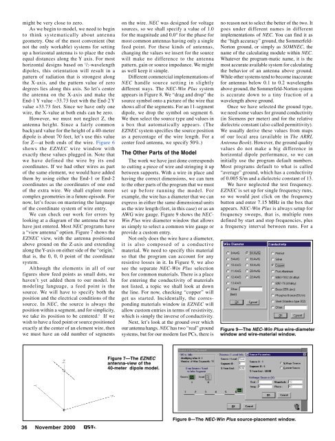
We can check our work for errors by
looking at a diagram of the antenna that we
have just entered. Most NEC programs have
a “view antenna” option. Figure 7 shows the
EZNEC view, with the antenna positioned
above ground on the Z-axis and extending
along the Y-axis on either side of the “origin,”
that is, the 0, 0, 0 point of the coordinate
system.
Although the elements in all of our
figures show feed points as small dots, we
haven’t yet added them to our model. In
modeling language, a feed point is the
source. We will have to specify both the
position and the electrical conditions of the
source. In NEC, the source is always the
position within a segment, and for simplicity,
we take its position to be centered. 6 If we
wish to have a feed point or source positioned
exactly at the center of an element wire, then
we must have an odd number of segments
on the wire. NEC was designed for voltage
sources, so we shall specify a value of 1.0
for the magnitude and 0.0° for the phase for
most common antennas having only a single
feed point. For these kinds of antennas,
changing the values we insert for the source
will make no difference to the antenna
pattern, gain or source impedance. We might
as well keep it simple.
Different commercial implementations of
NEC handle source setting in slightly
different ways. The NEC-Win Plus system
appears in Figure 8. We “drag and drop” the
source symbol onto a picture of the wire that
shows all of the segments. For an 11-segment
dipole, we drop the symbol on segment 6.
We then select the source type and values in
a box that automatically appears. (The
EZNEC system specifies the source position
as a percentage of the wire length. For a
center feed antenna, we specify 50%.)
The Other Parts of the Model
The work we have just done corresponds
to cutting a piece of wire and stringing it up
between supports. With a wire in place and
having the correct dimensions, we can turn
to the other parts of the program that we must
set up before running the model. For
example, the wire has a diameter that we can
express in either the same dimensional units
as the wire length (feet, in this case) or as an
AWG wire gauge. Figure 9 shows the NEC-
Win Plus wire diameter window that allows
us simply to select a common wire gauge or
provide a custom entry.
Not only does the wire have a diameter,
it is also composed of a conductive
material. We need to specify this material
so that the program can account for any
resistive losses in it. In Figure 9, we also
see the separate NEC-Win Plus selection
box for common materials. There is a place
for entering the conductivity of materials
not listed, a topic we shall look at down
the line. For now, checking “copper” will
get us started. Incidentally, the corresponding
materials window in EZNEC will
allow custom entries in terms of resistivity,
which is simply the inverse of conductivity.
Next, let’s look at the ground over which
our antenna hangs. NEC has two “real” ground
systems, but for our modern fast PCs, there is
no reason not to select the better of the two. It
goes under different names in different
implementations of NEC. You can find it as
the “high accuracy” ground, the Sommerfeld-
Norton ground, or simply as SOMNEC, the
name of the calculating module within NEC.
Whatever the program-matic name, it is the
most accurate available system for calculating
the behavior of an antenna above ground.
While other systems tend to become inaccurate
for antennas below 0.1 to 0.2 wavelengths
above ground, the Sommerfeld-Norton system
is accurate down to a tiny fraction of a
wavelength above ground.
Once we have selected the ground type,
we need some values for ground conductivity
(in Siemens per meter) and for the relative
dielectric constant (also called permittivity).
We usually derive these values from maps
of our local area (available in The ARRL
Antenna Book). However, the ground quality
values do not make a big difference in
horizontal dipole performance, so we can
initially use the program default numbers.
Most programs default to what is called
“average” ground, which has a conductivity
of 0.005 S/m and a dielectric constant of 13.
We have neglected the test frequency.
EZNEC is set up for single frequency runs,
so we would just click on the frequency
button and enter 7.15 MHz in the box that
appears. NEC-Win Plus is always setup for
frequency sweeps, that is, multiple runs
defined by start and stop frequencies, plus
a frequency interval between runs. For a
Figure 9—The NEC-Win Plus wire-diameter
window and wire-material window.
Figure 7—The EZNEC
antenna-view of the
40-meter dipole model.
36 November 2000
Figure 8—The NEC-Win Plus source-placement window.