Image Enhancement - Nubacad.com
Image Enhancement - Nubacad.com
Image Enhancement - Nubacad.com

You also want an ePaper? Increase the reach of your titles
YUMPU automatically turns print PDFs into web optimized ePapers that Google loves.
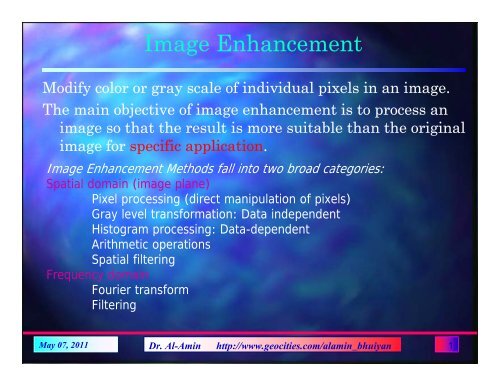
<strong>Image</strong> <strong>Enhancement</strong><br />
Modify color or gray scale of individual pixels in an image.<br />
The main objective of image enhancement is to process an<br />
image so that the result is more suitable than the original<br />
image for specific application.<br />
<strong>Image</strong> <strong>Enhancement</strong> Methods fall into two broad categories:<br />
Spatial domain (image plane)<br />
Pixel processing (direct manipulation of pixels)<br />
Gray level transformation: Data independent<br />
Histogram processing: Data-dependent<br />
Arithmetic operations<br />
Spatial filtering<br />
Frequency domain<br />
Fourier transform<br />
Filtering<br />
May 07, 2011 Dr. Al-Amin http://www.geocities.<strong>com</strong>/alamin_bhuiyan 1
Spatial Domain<br />
Spatial domain processes denoted as:<br />
g (x,y) = T [f (x,y)];<br />
where f (x,y) is the input image, g (x,y) is the processed image, T is<br />
the operator on f, defined over some neighborhood of (x,y).<br />
Gray Level Trans. Func.<br />
The simplest form of T is when<br />
the neighborhood size is 1x1<br />
(that is a single pixel). (Point<br />
Processing)<br />
s = T(r)<br />
r and s denote the gray level of f<br />
(x,y) and g (x,y) at point (x,y),<br />
respectively.<br />
May 07, 2011 Dr. Al-Amin http://www.geocities.<strong>com</strong>/alamin_bhuiyan 2
Gray Level Transformation Function: s = T(r)<br />
The effect of gray level transformation of Fig. 3.2 would be to<br />
produce an image of higher contrast than the original by<br />
darkening the levels below m and brightening the levels above<br />
m in the original image. This technique is known as contrast<br />
stretching.<br />
May 07, 2011 Dr. Al-Amin http://www.geocities.<strong>com</strong>/alamin_bhuiyan 3
Basic Gray-level Transforms<br />
• Operated on individual pixel’s intensity values:<br />
s = T(r). r: original intensity, s: new intensity<br />
• Data independent pixel-based enhancement<br />
method.<br />
• Approaches<br />
– <strong>Image</strong> negatives<br />
– Log transform<br />
– Power law transform<br />
– Piece-wise linear transform<br />
May 07, 2011 Dr. Al-Amin http://www.geocities.<strong>com</strong>/alamin_bhuiyan 4
<strong>Image</strong> Negatives<br />
• s = T(r) = L-1-r<br />
• Similar to photo negatives.<br />
• Suitable for enhancing gray details in dark background.<br />
May 07, 2011 Dr. Al-Amin http://www.geocities.<strong>com</strong>/alamin_bhuiyan 5
Log Gray-level Transform<br />
• s = T(r) = c log(1+r) • expand dark value to enhance<br />
details of dark area<br />
(a) Fourier spectrum and (b) Result of applying<br />
Log transform.<br />
May 07, 2011 Dr. Al-Amin http://www.geocities.<strong>com</strong>/alamin_bhuiyan 6
Piece-wise Linear Gray-level Transform<br />
• Allow more control on the <strong>com</strong>plexity of T(r).<br />
– Contrast stretching<br />
– Gray-level slicing<br />
– Bit-plane slicing<br />
Contrast stretching<br />
Low contrast images can result poor<br />
illumination, lack of dynamic range in the<br />
imaging sensor, or even wrong setting of<br />
imaging aperture during image acquisition.<br />
The idea behind contrast stretching is to<br />
increase the dynamic range of the gray<br />
levels in the image behind process.<br />
May 07, 2011 Dr. Al-Amin http://www.geocities.<strong>com</strong>/alamin_bhuiyan 7
Contrast Stretching<br />
Run program spatial_c.m<br />
May 07, 2011 Dr. Al-Amin http://www.geocities.<strong>com</strong>/alamin_bhuiyan 8
Gray-level Slicing<br />
Provides a binary image<br />
Gray level slicing is<br />
ac<strong>com</strong>plished by<br />
highlighting a specific<br />
range of gray levels in<br />
an image by displaying<br />
a high value for all gray<br />
levels in the range of<br />
interest and a low value<br />
for all other gray levels.<br />
Applications:<br />
Enhancing features<br />
such as masses of water<br />
in satellite imagery and<br />
enhancing flaws in x-<br />
ray images.<br />
May 07, 2011 Dr. Al-Amin http://www.geocities.<strong>com</strong>/alamin_bhuiyan 9
Bit-Slicing<br />
Provides highlighting<br />
the contribution made<br />
to total image<br />
appearance by specific<br />
bits.<br />
Suppose that each<br />
pixel in an image is<br />
represented by 8 bits.<br />
Imagine that the<br />
image is <strong>com</strong>posed of<br />
eight 1-bit planes,<br />
ranging from bit plane<br />
0 for the least<br />
significant bit to bit<br />
plane 7 for the most<br />
significant bit.<br />
May 07, 2011 Dr. Al-Amin http://www.geocities.<strong>com</strong>/alamin_bhuiyan 10
Histogram<br />
• The histogram of an image records the<br />
frequency distribution of gray levels in<br />
that image.<br />
• The histogram of a digital image with<br />
gray levels in the rage [0, L-1] is the<br />
discrete function h(r k ) = n k where r k is<br />
the k-th gray level and n k is the number<br />
of pixels in the image having gray level<br />
r k .<br />
• Normalized histogram<br />
p r (r k ) = n k /n, for k = 0,1,…, L-1<br />
• p(r k ) gives the estimates of the<br />
probability of occurrence of gray level<br />
r k .<br />
• A plot p(r k ) versus r k is called the<br />
Histogram<br />
• Several effects of histograms are shown<br />
at the right side.<br />
May 07, 2011 Dr. Al-Amin http://www.geocities.<strong>com</strong>/alamin_bhuiyan 11
Cumulative Histogram<br />
Records the cumulative<br />
frequency distribution of<br />
gray levels in an image.<br />
k<br />
nk<br />
sk<br />
= T ( r)<br />
= ∑<br />
n<br />
j=<br />
0<br />
The cumulative frequency of a gray<br />
level, i, is the number of times that a<br />
gray level less than or equal to i<br />
occurs in an image.<br />
May 07, 2011 Dr. Al-Amin http://www.geocities.<strong>com</strong>/alamin_bhuiyan 12
Histogram Equalization<br />
Redistribution of gray levels: an attempt to<br />
flatten the frequency distribution.<br />
The probability of occurrence of gray level r k ,<br />
p r (r k ) = n k /n, for k = 0,1,…, L-1;<br />
where n is the total number of pixels, r k is the<br />
k-th gray level and n k is the number of pixels<br />
having gray level r k .<br />
Then the Histogram Equalization or Histogram<br />
Linearization transformation function:<br />
k<br />
k<br />
n<br />
j<br />
sk<br />
= T ( rk<br />
) = ∑ pr<br />
( rj<br />
) = ∑ ;<br />
n<br />
j=<br />
0<br />
j=<br />
0<br />
for k = 0,1,2,..,L-1<br />
The function s can be considered as cumulative<br />
sum of p r (r k )<br />
More gray levels are allocated<br />
where there are most pixels,<br />
fewer gray levels where there<br />
fewer pixels.<br />
This tends to increase contrast in<br />
the most heavily populated<br />
regions of the histogram.<br />
May 07, 2011 Dr. Al-Amin http://www.geocities.<strong>com</strong>/alamin_bhuiyan 13
Histogram Equalization<br />
Histogram equalization<br />
be<strong>com</strong>es histogram<br />
specification, if instead<br />
of requiring a flat<br />
histogram, we specify<br />
a particular shape<br />
explicitly.<br />
May 07, 2011 Dr. Al-Amin http://www.geocities.<strong>com</strong>/alamin_bhuiyan 14
Histogram Equalization …<br />
May 07, 2011 Dr. Al-Amin http://www.geocities.<strong>com</strong>/alamin_bhuiyan 15
Histogram Equalization …<br />
• A gray-level transformation method that forces the transformed gray level to<br />
spread over the entire intensity range.<br />
– Data dependent,<br />
– (usually) Contrast enhanced<br />
• Usually, the discrete-valued histogram equalization algorithm does not yield<br />
exact uniform distribution of histogram.<br />
• In practice, one may prefer “histogram specification”<br />
May 07, 2011 Dr. Al-Amin http://www.geocities.<strong>com</strong>/alamin_bhuiyan 16
Enhancing using Arithmetic/Logic Operations<br />
May 07, 2011 Dr. Al-Amin http://www.geocities.<strong>com</strong>/alamin_bhuiyan 17
Enhancing using Arithmetic/Logic Operations<br />
May 07, 2011 Dr. Al-Amin http://www.geocities.<strong>com</strong>/alamin_bhuiyan 18
<strong>Image</strong> Subtraction<br />
Subtraction of two images result in a new image whose pixel at coordinates<br />
(x,y) is the difference between the pixels in that same<br />
location in the two images being subtracted.<br />
The difference between two images f(x,y) and h(x,y) is expresses by:<br />
g(x,y)= f(x,y) - h(x,y)<br />
May 07, 2011 Dr. Al-Amin http://www.geocities.<strong>com</strong>/alamin_bhuiyan 19
<strong>Image</strong> Subtraction<br />
May 07, 2011 Dr. Al-Amin http://www.geocities.<strong>com</strong>/alamin_bhuiyan 20