Econometrics II Problem Set 8 44709 – Group 2 (SOLUTIONS)

Econometrics II
Graduate School of Management and Economics
Problem Set 8
44709 – Group 2 (SOLUTIONS)
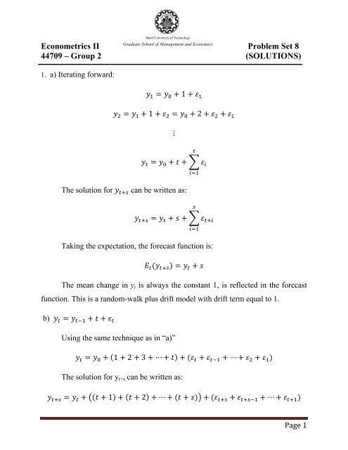
1. a) Iterating forward:
Sharif University of Technology
1
1 2
The solution for can be written as:
Taking the expectation, the forecast function is:
The mean change in y t is always the constant 1, is reflected in the forecast
function. This is a random-walk plus drift model with drift term equal to 1.
b)
Using the same technique as in “a)”
1 23
The solution for y t+s can be written as:
1 2
Page 1

The forecast function is:
1 2
1
2
Note that the change in y t is positively related to t. As such, the slope of the
forecast function is positively related to t.
c) Given initial conditions for all stochastic terms:
In period zero, the value of is given by: 0.5 (assume that μ 0 ,
η 0 and η -1 are known) so that we can write the model as:
0.5 0.5
The solution for y t+s can be written as:
0.5 0.5
Hence, the forecast function is:
0.5 0.5 1
0.5 1
Here y t is a random-walk plus a stationary component that is a MA(1) process.
Page 2

d) write as: Δy t = t + ε t . Now, simply detrend the Δy t sequence
to obtain a stationary sequence.
e) The model has an ARIMA(0,1,2) representation.
Recall that: 0.5 where . Differencing once
yields: 1 0.5 0.5 where is stationary.
The { } sequence is stationary as:
0,
1.5 , and all autocorrelations are constant.
The first order autocorrelation of is:
,
0.25
1.5
The second order autocorrelation of is:
,
0.5
1.5
The third order autocorrelation of is:
,
0
1.5 0
and: 0.
Thus, the autocorrelation function of has the same characteristics as an MA(2)
process, hence, has an ARIMA(0,1,2) representation.
Page 3