Cisco CCIE Fundamentals Network Design.PDF - Ostad Online

About This Manual 

Document Objectives 

This publication provides internetworking design and implementation information and helps you 

identify and implement practical internetworking strategies that are both flexible and scalable. 

This publication was developed to assist professionals preparing for Cisco Certified Internetwork 

Expert (CCIE) candidacy, though it is a valuable resource for all internetworking professionals. It is 

designed for use in conjunction with other Cisco manuals or as a standalone reference. You may find 

it helpful to refer to the Cisco CCIE Fundamentals: Case Studies, which provides case studies and 

examples of the network design strategies described in this book. 

Audience 

This publication is intended to support the network administrator who designs and implements 

router- or switched-based internetworks. 

Readers will better understand the material in this publication if they are familiar with networking 

terminology. The Cisco Internetworking Terms and Acronyms publication is a useful reference for 

those with minimal knowledge of networking terms. 

Document Organization 

This manual contains three parts, which are described below: 

Part I, “Overview,” provides an introduction to the type of internetworking design topics that will be 

discussed in this publication. 

Part II, “Design Concepts,” provides detailed information about each of the design strategies and 

technologies contained in this publication. 

Part III, “Appedixes,” contains reference material. 

Document Conventions 

In this publication, the following conventions are used: 

• Commands and keywords are in boldface. 

• New, important terms are italicized when accompanied by a definition or discussion of the term. 

• Protocol names are italicized at their first use in each chapter. 

About This Manual 

xix

Document Conventions 

Note Means reader take note. Notes contain helpful suggestions or references to materials not 

contained in this manual. 

xx 

Cisco CCIE Fundamentals: Network Design

CHAPTER 

1 

Introduction 

Internetworking—the communication between two or more networks—encompasses every aspect 

of connecting computers together. Internetworks have grown to support vastly disparate 

end-system communication requirements. An internetwork requires many protocols and features to 

permit scalability and manageability without constant manual intervention. Large internetworks can 

consist of the following three distinct components: 

• Campus networks, which consist of locally connected users in a building or group of buildings 

• Wide-area networks (WANs), which connect campuses together 

• Remote connections, which link branch offices and single users (mobile users and/or 

telecommuters) to a local campus or the Internet 

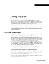
Figure 1-1 provides an example of a typical enterprise internetwork. 

Figure 1-1 

Example of a typical enterprise internetwork. 

WAN 

Campus 

Switch 

Campus 

Router A 

Switch 

WAN 

Router B 

LAN 

Switch 

LAN 

WAN 

Site 1 

Host A 

Host B 

Site 2 

Designing an internetwork can be a challenging task. To design reliable, scalable internetworks, 

network designers must realize that each of the three major components of an internetwork have 

distinct design requirements. An internetwork that consists of only 50 meshed routing nodes can 

pose complex problems that lead to unpredictable results. Attempting to optimize internetworks that 

feature thousands of nodes can pose even more complex problems. 

Introduction 1-1

Designing Campus Networks 

Despite improvements in equipment performance and media capabilities, internetwork design is 

becoming more difficult. The trend is toward increasingly complex environments involving multiple 

media, multiple protocols, and interconnection to networks outside any single organization’s 

dominion of control. Carefully designing internetworks can reduce the hardships associated with 

growth as a networking environment evolves. 

This chapter provides an overview of the technologies available today to design internetworks. 

Discussions are divided into the following general topics: 

• Designing Campus Networks 

• Designing WANs 

• Utilizing Remote Connection Design 

• Providing Integrated Solutions 

• Determining Your Internetworking Requirements 

Designing Campus Networks 

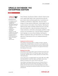
A campus is a building or group of buildings all connected into one enterprise network that consists 

of many local area networks (LANs). A campus is generally a portion of a company (or the whole 

company) constrained to a fixed geographic area, as shown in Figure 1-2. 

Figure 1-2 

Example of a campus network. 

WAN 

Router 

Building B 

Router 

Router 

Switch 

Building A 

Building C 

Token 

Ring 

Token 

Ring 

The distinct characteristic of a campus environment is that the company that owns the campus 

network usually owns the physical wires deployed in the campus. The campus network topology is 

primarily LAN technology connecting all the end systems within the building. Campus networks 

generally use LAN technologies, such as Ethernet, Token Ring, Fiber Distributed Data Interface 

(FDDI), Fast Ethernet, Gigabit Ethernet, and Asynchronous Transfer Mode (ATM). 

1-2 


Trends in Campus Design 

A large campus with groups of buildings can also use WAN technology to connect the buildings. 

Although the wiring and protocols of a campus might be based on WAN technology, they do not 

share the WAN constraint of the high cost of bandwidth. After the wire is installed, bandwidth is 

inexpensive because the company owns the wires and there is no recurring cost to a service provider. 

However, upgrading the physical wiring can be expensive. 

Consequently, network designers generally deploy a campus design that is optimized for the fastest 

functional architecture that runs on existing physical wire. They might also upgrade wiring to meet 

the requirements of emerging applications. For example, higher-speed technologies, such as Fast 

Ethernet, Gigabit Ethernet, and ATM as a backbone architecture, and Layer 2 switching provide 

dedicated bandwidth to the desktop. 

Trends in Campus Design 

In the past, network designers had only a limited number of hardware options—routers or 

hubs—when purchasing a technology for their campus networks. Consequently, it was rare to make 

a hardware design mistake. Hubs were for wiring closets and routers were for the data center or main 

telecommunications operations. 

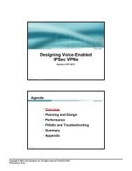
Recently, local-area networking has been revolutionized by the exploding use of LAN switching at 

Layer 2 (the data link layer) to increase performance and to provide more bandwidth to meet new 

data networking applications. LAN switches provide this performance benefit by increasing 

bandwidth and throughput for workgroups and local servers. Network designers are deploying LAN 

switches out toward the network’s edge in wiring closets. As Figure 1-3 shows, these switches are 

usually installed to replace shared concentrator hubs and give higher bandwidth connections to the 

end user. 

Figure 1-3 

Example of trends in campus design. 

Traditional wiring closet 

Shared hub 

Si 

Multilayer switch 

(Layers 2 and 3) 

The new wiring closet 

LAN switch (Layer 2) 

Hub 

Cisco router 

ATM campus 

switch 


CDDI/FDDI 

concentrator 

Traditional backbone 

The new backbone 

Shared hub 

Layer 3 networking is required in the network to interconnect the switched workgroups and to 

provide services that include security, quality of service (QoS), and traffic management. Routing 

integrates these switched networks, and provides the security, stability, and control needed to build 

functional and scalable networks. 

Introduction 1-3

Designing WANs 

Traditionally, Layer 2 switching has been provided by LAN switches, and Layer 3 networking has 

been provided by routers. Increasingly, these two networking functions are being integrated into 

common platforms. For example, multilayer switches that provide Layer 2 and 3 functionality are 

now appearing in the marketplace. 

With the advent of such technologies as Layer 3 switching, LAN switching, and virtual LANs 

(VLANs), building campus networks is becoming more complex than in the past. Table 1-1 

summarizes the various LAN technologies that are required to build successful campus networks. 

Cisco Systems offers product solutions in all of these technologies. 

Table 1-1 

Summary of LAN Technologies 

LAN Technology 

Routing technologies 

Gigabit Ethernet 

LAN switching technologies 

• Ethernet switching 

• Token Ring switching 

ATM switching technologies 

Typical Uses 

Routing is a key technology for connecting LANs in a campus network. It can be 

either Layer 3 switching or more traditional routing with Layer 3 switching and 

additional router features. 

Gigabit Ethernet builds on top of the Ethernet protocol, but increases speed ten-fold 

over Fast Ethernet to 1000 Mbps, or 1 Gbps. Gigabit Ethernet provides high 

bandwidth capacity for backbone designs while providing backward compatibility for 

installed media. 

Ethernet switching provides Layer 2 switching, and offers dedicated Ethernet 

segments for each connection. This is the base fabric of the network. 

Token Ring switching offers the same functionality as Ethernet switching, but uses 

Token Ring technology. You can use a Token Ring switch as either a transparent 

bridge or as a source-route bridge. 

ATM switching offers high-speed switching technology for voice, video, and data. Its 

operation is similar to LAN switching technologies for data operations. ATM, 

however, offers high bandwidth capacity. 

Network designers are now designing campus networks by purchasing separate equipment types (for 

example, routers, Ethernet switches, and ATM switches) and then linking them together. Although 

individual purchase decisions might seem harmless, network designers must not forget that the entire 

network forms an internetwork. 

It is possible to separate these technologies and build thoughtful designs using each new technology, 

but network designers must consider the overall integration of the network. If this overall integration 

is not considered, the result can be networks that have a much higher risk of network outages, 

downtime, and congestion than ever before. 

Designing WANs 

WAN communication occurs between geographically separated areas. In enterprise internetworks, 

WANs connect campuses together. When a local end station wants to communicate with a remote 

end station (an end station located at a different site), information must be sent over one or more 

WAN links. Routers within enterprise internetworks represent the LAN/WAN junction points of an 

internetwork. These routers determine the most appropriate path through the internetwork for the 

required data streams. 

WAN links are connected by switches, which are devices that relay information through the WAN 

and dictate the service provided by the WAN. WAN communication is often called a service because 

the network provider often charges users for the services provided by the WAN (called tariffs). WAN 

services are provided through the following three primary switching technologies: 

1-4 


Trends in WAN Design 

• Circuit switching 

• Packet switching 

• Cell switching 

Each switching technique has advantages and disadvantages. For example, circuit-switched 

networks offer users dedicated bandwidth that cannot be infringed upon by other users. In contrast, 

packet-switched networks have traditionally offered more flexibility and used network bandwidth 

more efficiently than circuit-switched networks. Cell switching, however, combines some aspects of 

circuit and packet switching to produce networks with low latency and high throughput. Cell 

switching is rapidly gaining in popularity. ATM is currently the most prominent cell-switched 

technology. For more information on switching technology for WANs and LANs, see Chapter 2, 

“Internetworking Design Basics.” 

Trends in WAN Design 

Traditionally, WAN communication has been characterized by relatively low throughput, high delay, 

and high error rates. WAN connections are mostly characterized by the cost of renting media (wire) 

from a service provider to connect two or more campuses together. Because the WAN infrastructure 

is often rented from a service provider, WAN network designs must optimize the cost of bandwidth 

and bandwidth efficiency. For example, all technologies and features used to connect campuses over 

a WAN are developed to meet the following design requirements: 

• Optimize WAN bandwidth 

• Minimize the tariff cost 

• Maximize the effective service to the end users 

Recently, traditional shared-media networks are being overtaxed because of the following new 

network requirements: 

• Necessity to connect to remote sites 

• Growing need for users to have remote access to their networks 

• Explosive growth of the corporate intranets 

• Increased use of enterprise servers 

Network designers are turning to WAN technology to support these new requirements. WAN 

connections generally handle mission-critical information, and are optimized for price/performance 

bandwidth. The routers connecting the campuses, for example, generally apply traffic optimization, 

multiple paths for redundancy, dial backup for disaster recovery, and QoS for critical applications. 

Table 1-2 summarizes the various WAN technologies that support such large-scale internetwork 

requirements. 

Table 1-2 

Summary of WAN Technologies 

WAN Technology 

Asymmetric Digital Subscriber Line 

Analog modem 

Typical Uses 

A new modem technology. Converts existing twisted-pair telephone 

lines into access paths for multimedia and high-speed data 

communications. ADSL transmits more than 6 Mbps to a 

subscriber, and as much as 640 kbps more in both directions. 

Analog modems can be used by telecommuters and mobile users 

who access the network less than two hours per day, or for backup 

for another type of link. 

Introduction 1-5

Utilizing Remote Connection Design 

Leased line 

Integrated Services Digital Network (ISDN) 

Frame Relay 

Switched Multimegabit Data Service (SMDS) 

Leased lines can be used for Point-to-Point Protocol (PPP) networks 

and hub-and-spoke topologies, or for backup for another type of link. 

ISDN can be used for cost-effective remote access to corporate 

networks. It provides support for voice and video as well as a backup 

for another type of link. 

Frame Relay provides a cost-effective, high- speed, low-latency 

mesh topology between remote sites. It can be used in both private 

and carrier-provided networks. 

SMDS provides high-speed, high-performance connections across 

public data networks. It can also be deployed in metropolitan-area 

networks (MANs). 

X.25 X.25 can provide a reliable WAN circuit or backbone. It also 

provides support for legacy applications. 

WAN ATM 

WAN ATM can be used to accelerate bandwidth requirements. It also 

provides support for multiple QoS classes for differing application 

requirements for delay and loss. 

Utilizing Remote Connection Design 

Remote connections link single users (mobile users and/or telecommuters) and branch offices to a 

local campus or the Internet. Typically, a remote site is a small site that has few users and therefore 

needs a smaller size WAN connection. The remote requirements of an internetwork, however, 

usually involve a large number of remote single users or sites, which causes the aggregate WAN 

charge to be exaggerated. 

Because there are so many remote single users or sites, the aggregate WAN bandwidth cost is 

proportionally more important in remote connections than in WAN connections. Given that the 

three-year cost of a network is nonequipment expenses, the WAN media rental charge from a service 

provider is the largest cost component of a remote network. Unlike WAN connections, smaller sites 

or single users seldom need to connect 24 hours a day. 

Consequently, network designers typically choose between dial-up and dedicated WAN options for 

remote connections. Remote connections generally run at speeds of 128 Kbps or lower. A network 

designer might also employ bridges in a remote site for their ease of implementation, simple 

topology, and low traffic requirements. 

Trends in Remote Connections 

Today, there is a large selection of remote WAN media that include the following: 

• Analog modem 

• Asymmetric Digital Subscriber Line 

• Leased line 

• Frame Relay 

• X.25 

• ISDN 

Remote connections also optimize for the appropriate WAN option to provide cost-effective 

bandwidth, minimize dial-up tariff costs, and maximize effective service to users. 

1-6 


Trends in LAN/WAN Integration 

Trends in LAN/WAN Integration 

Today, 90 percent of computing power resides on desktops, and that power is growing exponentially. 

Distributed applications are increasingly bandwidth hungry, and the emergence of the Internet is 

driving many LAN architectures to the limit. Voice communications have increased significantly 

with more reliance on centralized voice mail systems for verbal communications. The internetwork 

is the critical tool for information flow. Internetworks are being pressured to cost less, yet support 

the emerging applications and higher number of users with increased performance. 

To date, local- and wide-area communications have remained logically separate. In the LAN, 

bandwidth is free and connectivity is limited only by hardware and implementation costs. The LAN 

has carried data only. In the WAN, bandwidth has been the overriding cost, and such delay-sensitive 

traffic as voice has remained separate from data. New applications and the economics of supporting 

them, however, are forcing these conventions to change. 

The Internet is the first source of multimedia to the desktop, and immediately breaks the rules. Such 

Internet applications as voice and real-time video require better, more predictable LAN and WAN 

performance. These multimedia applications are fast becoming an essential part of the business 

productivity toolkit. As companies begin to consider implementing new intranet-based, bandwidthintensive 

multimedia applications—such as video training, videoconferencing, and voice over 

IP—the impact of these applications on the existing networking infrastructure is a serious concern. 

If a company has relied on its corporate network for business-critical SNA traffic, for example, and 

wants to bring a new video training application on line, the network must be able to provide 

guaranteed quality of service (QoS) that delivers the multimedia traffic, but does not allow it to 

interfere with the business-critical traffic. ATM has emerged as one of the technologies for 

integrating LANs and WANs. The Quality of Service (QoS) features of ATM can support any traffic 

type in separate or mixed streams, delay sensitive traffic, and nondelay-sensitive traffic, as shown in 

Figure 1-4. 

ATM can also scale from low to high speeds. It has been adopted by all the industry’s equipment 

vendors, from LAN to private branch exchange (PBX). 

Figure 1-4 

ATM support of various traffic types. 

PBX 

Circuit 

FEP 

Streams 

Cell switching 

LAN 

SNA 

Frames 

Packet 

Q 

Cells 

Cells 

ATM 

Introduction 1-7

Providing Integrated Solutions 

Providing Integrated Solutions 

The trend in internetworking is to provide network designers greater flexibility in solving multiple 

internetworking problems without creating multiple networks or writing off existing data 

communication investments. Routers might be relied upon to provide a reliable, secure network and 

act as a barrier against inadvertent broadcast storms in the local networks. Switches, which can be 

divided into two main categories—LAN switches and WAN switches—can be deployed at the 

workgroup, campus backbone, or WAN level. Remote sites might use low-end routers for connection 

to the WAN. 

Underlying and integrating all Cisco products is the Cisco Internetworking Operating System (Cisco 

IOS) software. The Cisco IOS software enables disparate groups, diverse devices, and multiple 

protocols all to be integrated into a highly reliable and scalable network. Cisco IOS software also 

supports this internetwork with advanced security, quality of service, and traffic services. 

Determining Your Internetworking Requirements 

Designing an internetwork can be a challenging task. Your first step is to understand your 

internetworking requirements. The rest of this chapter is intended as a guide for helping you 

determine these requirements. After you have identified these requirements, refer to Chapter 2, 

“Internetworking Design Basics,” for information on selecting internetwork capability and 

reliability options that meet these requirements. 

Internetworking devices must reflect the goals, characteristics, and policies of the organizations in 

which they operate. Two primary goals drive internetworking design and implementation: 

• Application availability—Networks carry application information between computers. If the 

applications are not available to network users, the network is not doing its job. 

• Cost of ownership—Information system (IS) budgets today often run in the millions of dollars. 

As large organizations increasingly rely on electronic data for managing business activities, the 

associated costs of computing resources will continue to rise. 

A well-designed internetwork can help to balance these objectives. When properly implemented, the 

network infrastructure can optimize application availability and allow the cost-effective use of 

existing network resources. 

The Design Problem: Optimizing Availability and Cost 

In general, the network design problem consists of the following three general elements: 

• Environmental givens—Environmental givens include the location of hosts, servers, terminals, 

and other end nodes; the projected traffic for the environment; and the projected costs for 

delivering different service levels. 

• Performance constraints—Performance constraints consist of network reliability, traffic 

throughput, and host/client computer speeds (for example, network interface cards and hard drive 

access speeds). 

• Internetworking variables—Internetworking variables include the network topology, line 

capacities, and packet flow assignments. 

The goal is to minimize cost based on these elements while delivering service that does not 

compromise established availability requirements. You face two primary concerns: availability and 

cost. These issues are essentially at odds. Any increase in availability must generally be reflected as 

an increase in cost. As a result, you must weigh the relative importance of resource availability and 

overall cost carefully. 

1-8 



As Figure 1-5 shows, designing your network is an iterative activity. The discussions that follow 

outline several areas that you should carefully consider when planning your internetworking 

implementation. 

Figure 1-5 

General network design process. 

Assess needs and costs 

Select topologies and 

technologies to satisfy needs 

Model network workload 

Simulate behavior under expected load 

Perform sensitivity tests 

Rework design as needed 

Assessing User Requirements 

In general, users primarily want application availability in their networks. The chief components of 

application availability are response time, throughput, and reliability: 

• Response time is the time between entry of a command or keystroke and the host system’s 

execution of the command or delivery of a response. User satisfaction about response time is 

generally considered to be a monotonic function up to some limit, at which point user satisfaction 

falls off to nearly zero. Applications in which fast response time is considered critical include 

interactive online services, such as automated tellers and point-of-sale machines. 

• Applications that put high-volume traffic onto the network have more effect on throughput than 

end-to-end connections. Throughput-intensive applications generally involve file- transfer 

activities. However, throughput-intensive applications also usually have low response-time 

requirements. Indeed, they can often be scheduled at times when 

response-time-sensitive traffic is low (for example, after normal work hours). 

• Although reliability is always important, some applications have genuine requirements that 

exceed typical needs. Organizations that require nearly 100 percent up time conduct all activities 

online or over the telephone. Financial services, securities exchanges, and 

emergency/police/military operations are a few examples. These situations imply a requirement 

for a high level of hardware and topological redundancy. Determining the cost of any downtime 

is essential in determining the relative importance of reliability to your internetwork. 

Introduction 1-9

Determining Your Internetworking Requirements 

You can assess user requirements in a number of ways. The more involved your users are in the 

process, the more likely that your evaluation will be accurate. In general, you can use the following 

methods to obtain this information: 

• User community profiles—Outline what different user groups require. This is the first step in 

determining internetwork requirements. Although many users have roughly the same 

requirements of an electronic mail system, engineering groups using XWindows terminals and 

Sun workstations in an NFS environment have different needs from PC users sharing print 

servers in a finance department. 

• Interviews, focus groups, and surveys—Build a baseline for implementing an internetwork. 

Understand that some groups might require access to common servers. Others might want to 

allow external access to specific internal computing resources. Certain organizations might 

require IS support systems to be managed in a particular way according to some external 

standard. The least formal method of obtaining information is to conduct interviews with key 

user groups. Focus groups can also be used to gather information and generate discussion among 

different organizations with similar (or dissimilar) interests. Finally, formal surveys can be used 

to get a statistically valid reading of user sentiment regarding a particular service level or 

proposed internetworking architecture. 

• Human factors tests—The most expensive, time-consuming, and possibly revealing method is to 

conduct a test involving representative users in a lab environment. This is most applicable when 

evaluating response time requirements. As an example, you might set up working systems and 

have users perform normal remote host activities from the lab network. By evaluating user 

reactions to variations in host responsiveness, you can create benchmark thresholds for 

acceptable performance. 

Assessing Proprietary and Nonproprietary Solutions 

Compatibility, conformance, and interoperability are related to the problem of balancing proprietary 

functionality and open internetworking flexibility. As a network designer, you might be forced to 

choose between implementing a multivendor environment and implementing a specific, proprietary 

capability. For example, the Interior Gateway Routing Protocol (IGRP) provides many useful 

capabilities, such as a number of features that are designed to enhance its stability. These include 

hold-downs, split horizons, and poison reverse updates. 

The negative side is that IGRP is a proprietary routing protocol. In contrast, the integrated 

Intermediate System-to Intermediate System (IS-IS) protocol is an open internetworking alternative 

that also provides a fast converging routing environment; however, implementing an open routing 

protocol can potentially result in greater multiple-vendor configuration complexity. 

The decisions that you make have far-ranging effects on your overall internetwork design. Assume 

that you decide to implement integrated IS-IS instead of IGRP. In doing this, you gain a measure of 

interoperability; however, you lose some functionality. For instance, you cannot load balance traffic 

over unequal parallel paths. Similarly, some modems provide a high level of proprietary diagnostic 

capabilities, but require that all modems throughout a network be of the same vendor type to fully 

exploit proprietary diagnostics. 

Previous internetworking (and networking) investments and expectations for future requirements 

have considerable influence over your choice of implementations. You need to consider installed 

internetworking and networking equipment; applications running (or to be run) on the network; 

traffic patterns; physical location of sites, hosts, and users; rate of growth of the user community; and 

both physical and logical network layout. 

1-10 



Assessing Costs 

The internetwork is a strategic element in your overall information system design. As such, the cost 

of your internetwork is much more than the sum of your equipment purchase orders. View it as a 

total cost-of-ownership issue. You must consider the entire life cycle of your internetworking 

environment. A brief list of costs associated with internetworks follows: 

• Equipment hardware and software costs—Consider what is really being bought when you 

purchase your systems; costs should include initial purchase and installation, maintenance, and 

projected upgrade costs. 

• Performance tradeoff costs—Consider the cost of going from a five-second response time to a 

half-second response time. Such improvements can cost quite a bit in terms of media selection, 

network interfaces, internetworking nodes, modems, and WAN services. 

• Installation costs—Installing a site’s physical cable plant can be the most expensive element of 

a large network. The costs include installation labor, site modification, fees associated with local 

code conformance, and costs incurred to ensure compliance with environmental restrictions 

(such as asbestos removal). Other important elements in keeping your costs to a minimum will 

include developing a well-planned wiring closet layout and implementing color code conventions 

for cable runs. 

• Expansion costs—Calculate the cost of ripping out all thick Ethernet, adding additional 

functionality, or moving to a new location. Projecting your future requirements and accounting 

for future needs saves time and money. 

• Support costs—Complicated internetworks cost more to monitor, configure, and maintain. Your 

internetwork should be no more complicated than necessary. Costs include training, direct labor 

(network managers and administrators), sparing, and replacement costs. Additional cost that 

should be included is out-of-band management, SNMP management stations, and power. 

• Cost of downtime—Evaluate the cost for every minute that a user is unable to access a file server 

or a centralized database. If this cost is high, you must attribute a high cost to downtime. If the 

cost is high enough, fully redundant internetworks might be your best option. 

• Opportunity costs—Every choice you make has an opposing alternative option. Whether that 

option is a specific hardware platform, topology solution, level of redundancy, or system 

integration alternative, there are always options. Opportunity costs are the costs of not picking 

one of those options. The opportunity costs of not switching to newer technologies and 

topologies might be lost competitive advantage, lower productivity, and slower overall 

performance. Any effort to integrate opportunity costs into your analysis can help to make 

accurate comparisons at the beginning of your project. 

• Sunken costs—Your investment in existing cable plant, routers, concentrators, switches, hosts, 

and other equipment and software are your sunken costs. If the sunken cost is high, you might 

need to modify your networks so that your existing internetwork can continue to be utilized. 

Although comparatively low incremental costs might appear to be more attractive than significant 

redesign costs, your organization might pay more in the long run by not upgrading systems. Over 

reliance on sunken costs can cost your organization sales and market share when calculating the 

cost of internetwork modifications and additions. 

Estimating Traffic: Work Load Modeling 

Empirical work-load modeling consists of instrumenting a working internetwork and monitoring 

traffic for a given number of users, applications, and network topology. Try to characterize activity 

throughout a normal work day in terms of the type of traffic passed, level of traffic, response time of 

hosts, time to execute file transfers, and so on. You can also observe utilization on existing network 

equipment over the test period. 

Introduction 1-11

Summary 

If the tested internetwork’s characteristics are close to the new internetwork, you can try 

extrapolating to the new internetwork’s number of users, applications, and topology. This is a 

best-guess approach to traffic estimation given the unavailability of tools to characterize detailed traffic 

behavior. 

In addition to passive monitoring of an existing network, you can measure activity and traffic 

generated by a known number of users attached to a representative test network and then extrapolate 

findings to your anticipated population. 

One problem with modeling workloads on networks is that it is difficult to accurately pinpoint traffic 

load and network device performance as functions of the number of users, type of application, and 

geographical location. This is especially true without a real network in place. Consider the following 

factors that influence the dynamics of the network: 

• The time-dependent nature of network access—Peak periods can vary; measurements must 

reflect a range of observations that includes peak demand. 

• Differences associated with type of traffic—Routed and bridged traffic place different demands 

on internetwork devices and protocols; some protocols are sensitive to dropped packets; some 

application types require more bandwidth. 

• The random (nondeterministic) nature of network traffic—Exact arrival time and specific effects 

of traffic are unpredictable. 

Sensitivity Testing 

From a practical point of view, sensitivity testing involves breaking stable links and observing what 

happens. When working with a test network, this is relatively easy. Disturb the network by removing 

an active interface, and monitor how the change is handled by the internetwork: how traffic is 

rerouted, the speed of convergence, whether any connectivity is lost, and whether problems arise in 

handling specific types of traffic. You can also change the level of traffic on a network to determine 

the effects on the network when traffic levels approach media saturation. This empirical testing is a 

type of regression testing: A series of specific modifications (tests) are repeated on different versions 

of network configurations. By monitoring the effects on the design variations, you can characterize 

the relative resilience of the design. 

Note Modeling sensitivity tests using a computer is beyond the scope of this publication. A useful 

source for more information about computer-based network design and simulation is 

A.S. Tannenbaum, Computer Networks, Upper Saddle River, New Jersey: Prentice Hall, 1996. 

Summary 

1-12 

After you have determined your network requirements, you must identify and then select the specific 

capability that fits your computing environment. For basic information on the different types of 

internetworking devices along with a description of a hierarchical approach to internetworking, refer 

to Chapter 2, “Internetworking Design Basics.” 

Chapters 2–13 in this book are technology chapters that present detailed discussions about specific 

implementations of large-scale internetworks in the following environments: 

• Large-scale Internetwork Protocol (IP) internetworks 

— Enhanced Interior Gateway Routing Protocol (IGRP) design 

— Open Shortest Path First (OSPF) design 

• IBM System Network Architecture (SNA) internetworks 


Summary 

— Source-route bridging (SRB) design 

— Synchronous Data Link Control (SDLC) and serial tunneling (STUN), SDLC Logical Link 

Control type 2 (SDLLC), and Qualified Logical Link Control (QLLC) design 

— Advanced Peer-to-Peer Networking (APPN) and Data Link Switching (DLSw) design 

• ATM internetworks 

• Packet service internetworks 

— Frame Relay design 

• Dial-on-demand routing (DDR) internetworks 

• ISDN internetworks 

In addition to these technology chapters there are chapters on designing switched LAN 

internetworks, campus LANs, and internetworks for multimedia applications. The last 12 chapters 

of this book include case studies relating to the concepts learned in the previous chapters. 

Introduction 1-13

Summary 

1-14 


CHAPTER 

2 

Internetworking Design Basics 

Designing an internetwork can be a challenging task. An internetwork that consists of only 

50 meshed routing nodes can pose complex problems that lead to unpredictable results. Attempting 

to optimize internetworks that feature thousands of nodes can pose even more complex problems. 

Despite improvements in equipment performance and media capabilities, internetwork design is 

becoming more difficult. The trend is toward increasingly complex environments involving multiple 

media, multiple protocols, and interconnection to networks outside any single organization’s 

dominion of control. Carefully designing internetworks can reduce the hardships associated with 

growth as a networking environment evolves. 

This chapter provides an overview of planning and design guidelines. Discussions are divided into 

the following general topics: 

• Understanding Basic Internetworking Concepts 

• Identifying and Selecting Internetworking Capabilities 

• Identifying and Selecting Internetworking Devices 

Understanding Basic Internetworking Concepts 

This section covers the following basic internetworking concepts: 

• Overview of Internetworking Devices 

• Switching Overview 

Overview of Internetworking Devices 

Network designers faced with designing an internetwork have four basic types of internetworking 

devices available to them: 

• Hubs (concentrators) 

• Bridges 

• Switches 

• Routers 

Table 2-1 summarizes these four internetworking devices. 

Internetworking Design Basics 2-1

Understanding Basic Internetworking Concepts 

Table 2-1 

Device 

Summary of Internetworking Devices 

Description 

Hubs (concentrators) 

Bridges 

Switches 

Routers 

Hubs (concentrators) are used to connect multiple users to a single physical device, which 

connects to the network. Hubs and concentrators act as repeaters by regenerating the signal as 

it passes through them. 

Bridges are used to logically separate network segments within the same network. They 

operate at the OSI data link layer (Layer 2) and are independent of higher-layer protocols. 

Switches are similar to bridges but usually have more ports. Switches provide a unique 

network segment on each port, thereby separating collision domains. Today, network 

designers are replacing hubs in their wiring closets with switches to increase their network 

performance and bandwidth while protecting their existing wiring investments. 

Routers separate broadcast domains and are used to connect different networks. Routers direct 

network traffic based on the destination network layer address (Layer 3) rather than the 

workstation data link layer or MAC address. Routers are protocol dependent. 

Data communications experts generally agree that network designers are moving away from bridges 

and concentrators and primarily using switches and routers to build internetworks. Consequently, 

this chapter focuses primarily on the role of switches and routers in internetwork design. 

Switching Overview 

Today in data communications, all switching and routing equipment perform two basic operations: 

• Switching data frames—This is generally a store-and-forward operation in which a frame arrives 

on an input media and is transmitted to an output media. 

• Maintenance of switching operations—In this operation, switches build and maintain switching 

tables and search for loops. Routers build and maintain both routing tables and service tables. 

There are two methods of switching data frames: Layer 2 and Layer 3 switching. 

Layer 2 and Layer 3 Switching 

Switching is the process of taking an incoming frame from one interface and delivering it out 

through another interface. Routers use Layer 3 switching to route a packet, and switches (Layer 2 

switches) use Layer 2 switching to forward frames. 

The difference between Layer 2 and Layer 3 switching is the type of information inside the frame 

that is used to determine the correct output interface. With Layer 2 switching, frames are 

switched based on MAC address information. With Layer 3 switching, frames are switched based 

on network-layer information. 

Layer 2 switching does not look inside a packet for network-layer information as does Layer 3 

switching. Layer 2 switching is performed by looking at a destination MAC address within a frame. 

It looks at the frame’s destination address and sends it to the appropriate interface if it knows the 

destination address location. Layer 2 switching builds and maintains a switching table that keeps 

track of which MAC addresses belong to each port or interface. 

If the Layer 2 switch does not know where to send the frame, it broadcasts the frame out all its ports 

to the network to learn the correct destination. When the frame’s reply is returned, the switch learns 

the location of the new address and adds the information to the switching table. 

2-2 


Switching Overview 

Layer 2 addresses are determined by the manufacturer of the data communications equipment used. 

They are unique addresses that are derived in two parts: the manufacturing (MFG) code and the 

unique identifier. The MFG code is assigned to each vendor by the IEEE. The vendor assigns a 

unique identifier to each board it produces. Except for Systems Network Architecture (SNA) 

networks, users have little or no control over Layer 2 addressing because Layer 2 addresses are fixed 

with a device, whereas Layer 3 addresses can be changed. In addition, Layer 2 addresses assume a 

flat address space with universally unique addresses. 

Layer 3 switching operates at the network layer. It examines packet information and forwards 

packets based on their network-layer destination addresses. Layer 3 switching also supports router 

functionality. 

For the most part, Layer 3 addresses are determined by the network administrator who installs a 

hierarchy on the network. Protocols such as IP, IPX, and AppleTalk use Layer 3 addressing. By 

creating Layer 3 addresses, a network administrator creates local areas that act as single addressing 

units (similar to streets, cities, states, and countries), and assigns a number to each local entity. If 

users move to another building, their end stations will obtain new Layer 3 addresses, but their Layer 

2 addresses remain the same. 

As routers operate at Layer 3 of the OSI model, they can adhere to and formulate a hierarchical 

addressing structure. Therefore, a routed network can tie a logical addressing structure to a physical 

infrastructure, for example, through TCP/IP subnets or IPX networks for each segment. Traffic flow 

in a switched (flat) network is therefore inherently different from traffic flow in a routed 

(hierarchical) network. Hierarchical networks offer more flexible traffic flow than flat networks 

because they can use the network hierarchy to determine optimal paths and contain broadcast 

domains. 

Implications of Layer 2 and Layer 3 Switching 

The increasing power of desktop processors and the requirements of client-server and multimedia 

applications have driven the need for greater bandwidth in traditional shared-media environments. 

These requirements are prompting network designers to replace hubs in wiring closets with 

switches. 

Although Layer 2 switches use microsegmentation to satisfy the demands for more bandwidth and 

increased performance, network designers are now faced with increasing demands for intersubnet 

communication. For example, every time a user accesses servers and other resources, which are 

located on different subnets, the traffic must go through a Layer 3 device. Figure 2-1 shows the route 

of intersubnet traffic with Layer 2 switches and Layer 3 switches. 

Figure 2-1 

Flow of intersubnet traffic with Layer 2 switches and routers. 

Client X 

Subnet 1 

Switch A 

Layer 2 switch 

Router A 


Switch B 


Server Y 

Subnet 2 

As Figure 2-1 shows, for Client X to communicate with Server Y, which is on another subnet, it must 

traverse through the following route: first through Switch A (a Layer 2 switch) and then through 

Router A (a Layer 3 switch) and finally through Switch B (a Layer 2 switch). Potentially there is a 

tremendous bottleneck, which can threaten network performance, because the intersubnet traffic 

must pass from one network to another. 


Identifying and Selecting Internetworking Capabilities 

To relieve this bottleneck, network designers can add Layer 3 capabilities throughout the network. 

They are implementing Layer 3 switching on edge devices to alleviate the burden on centralized 

routers. Figure 2-2 illustrates how deploying Layer 3 switching throughout the network allows 

Client X to directly communicate with Server Y without passing through Router A. 

Figure 2-2 

Flow of intersubnet traffic with Layer 3 switches. 

Client X 

Si 

Switch A 

Layer 2 and 3 switching 

Switch B 

Layer 2 and 3 switch 

Si 

Si 

Switch C 

Layer 2 and 3 switching 

Server Y 

Router A 


After you understand your internetworking requirements, you must identify and then select the 

specific capabilities that fit your computing environment. The following discussions provide a 

starting point for making these decisions: 

• Identifying and Selecting an Internetworking Model 

• Choosing Internetworking Reliability Options 

Identifying and Selecting an Internetworking Model 

Hierarchical models for internetwork design allow you to design internetworks in layers. To 

understand the importance of layering, consider the Open System Interconnection (OSI) reference 

model, which is a layered model for understanding and implementing computer communications. 

By using layers, the OSI model simplifies the task required for two computers to communicate. 

Hierarchical models for internetwork design also uses layers to simplify the task required for 

internetworking. Each layer can be focused on specific functions, thereby allowing the networking 

designer to choose the right systems and features for the layer. 

Using a hierarchical design can facilitate changes. Modularity in network design allows you to create 

design elements that can be replicated as the network grows. As each element in the network design 

requires change, the cost and complexity of making the upgrade is constrained to a small subset of 

the overall network. In large flat or meshed network architectures, changes tend to impact a large 

number of systems. Improved fault isolation is also facilitated by modular structuring of the network 

into small, easy-to-understand elements. Network mangers can easily understand the transition 

points in the network, which helps identify failure points. 

Using the Hierarchical Design Model 

A hierarchical network design includes the following three layers: 

2-4 


Using the Hierarchical Design Model 

• The backbone (core) layer that provides optimal transport between sites 

• The distribution layer that provides policy-based connectivity 

• The local-access layer that provides workgroup/user access to the network 

Figure 2-3 shows a high-level view of the various aspects of a hierarchical network design. A 

hierarchical network design presents three layers—core, distribution, and access—with each layer 

providing different functionality. 

Figure 2-3 

Hierarchical network design model. 

Core 

Distribution 

High-speed switching 

Access 

Policy-based connectivity 

Local and remote workgroup access 

Function of the Core Layer 

The core layer is a high-speed switching backbone and should be designed to switch packets as fast 

as possible. This layer of the network should not perform any packet manipulation, such as access 

lists and filtering, that would slow down the switching of packets. 

Function of the Distribution Layer 

The distribution layer of the network is the demarcation point between the access and core layers 

and helps to define and differentiate the core. The purpose of this layer is to provide boundary 

definition and is the place at which packet manipulation can take place. In the campus environment, 

the distribution layer can include several functions, such as the following: 

• Address or area aggregation 

• Departmental or workgroup access 

• Broadcast/multicast domain definition 

• Virtual LAN (VLAN) routing 

• Any media transitions that need to occur 

• Security 

In the non-campus environment, the distribution layer can be a redistribution point between routing 

domains or the demarcation between static and dynamic routing protocols. It can also be the point 

at which remote sites access the corporate network. The distribution layer can be summarized as the 

layer that provides policy-based connectivity. 



Function of the Access Layer 

The access layer is the point at which local end users are allowed into the network. This layer may 

also use access lists or filters to further optimize the needs of a particular set of users. In the campus 

environment, access-layer functions can include the following: 

• Shared bandwidth 

• Switched bandwidth 

• MAC layer filtering 

• Microsegmentation 

In the non-campus environment, the access layer can give remote sites access to the corporate 

network via some wide-area technology, such as Frame Relay, ISDN, or leased lines. 

It is sometimes mistakenly thought that the three layers (core, distribution, and access) must exist in 

clear and distinct physical entities, but this does not have to be the case. The layers are defined to aid 

successful network design and to represent functionality that must exist in a network. The 

instantiation of each layer can be in distinct routers or switches, can be represented by a physical 

media, can be combined in a single device, or can be omitted altogether. The way the layers are 

implemented depends on the needs of the network being designed. Note, however, that for a network 

to function optimally, hierarchy must be maintained. 

The discussions that follow outline the capabilities and services associated with backbone, 

distribution, and local access internetworking services. 

Evaluating Backbone Services 

This section addresses internetworking features that support backbone services. The following 

topics are discussed: 

• Path Optimization 

• Traffic Prioritization 

• Load Balancing 

• Alternative Paths 

• Switched Access 

• Encapsulation (Tunneling) 

Path Optimization 

One of the primary advantages of a router is its capability to help you implement a logical 

environment in which optimal paths for traffic are automatically selected. Routers rely on routing 

protocols that are associated with the various network layer protocols to accomplish this automated 

path optimization. 

Depending on the network protocols implemented, routers permit you to implement routing 

environments that suit your specific requirements. For example, in an IP internetwork, Cisco routers 

can support all widely implemented routing protocols, including Open Shortest Path First (OSPF), 

RIP, IGRP, Border Gateway Protocol (BGP), Exterior Gateway Protocol (EGP), and HELLO. Key 

built-in capabilities that promote path optimization include rapid and controllable route convergence 

and tunable routing metrics and timers. 

2-6 



Convergence is the process of agreement, by all routers, on optimal routes. When a network event 

causes routes to either halt operation or become available, routers distribute routing update 

messages. Routing update messages permeate networks, stimulating recalculation of optimal routes 

and eventually causing all routers to agree on these routes. Routing algorithms that converge slowly 

can cause routing loops or network outages. 

Many different metrics are used in routing algorithms. Some sophisticated routing algorithms base 

route selection on a combination of multiple metrics, resulting in the calculation of a single hybrid 

metric. IGRP uses one of the most sophisticated distance vector routing algorithms. It combines 

values for bandwidth, load, and delay to create a composite metric value. Link state routing 

protocols, such as OSPF and IS-IS, employ a metric that represents the cost associated with a given 

path. 

Traffic Prioritization 

Although some network protocols can prioritize internal homogeneous traffic, the router prioritizes 

the heterogeneous traffic flows. Such traffic prioritization enables policy-based routing and ensures 

that protocols carrying mission-critical data take precedence over less important traffic. 

Priority Queuing 

Priority queuing allows the network administrator to prioritize traffic. Traffic can be classified 

according to various criteria, including protocol and subprotocol type, and then queued on one of 

four output queues (high, medium, normal, or low priority). For IP traffic, additional fine-tuning is 

possible. Priority queuing is most useful on low-speed serial links. Figure 2-4 shows how priority 

queuing can be used to segregate traffic by priority level, speeding the transit of certain packets 

through the network. 

Figure 2-4 

Priority queuing. 

Router 

Traffic 

Priority 

Traffic sent to router 

without any priority 

UDP 

Bridged LAT 

DECnet 

VINES 

TCP 

Other bridged 

All other traffic 

AppleTalk 

High 

priority 

Medium 

priority 

Normal 

priority 

Low 

priority 

Backbone 

network 

Traffic sent to 

backbone in 

order of priority 

You can also use intraprotocol traffic prioritization techniques to enhance internetwork 

performance. IP’s type-of-service (TOS) feature and prioritization of IBM logical units (LUs) 

are intraprotocol prioritization techniques that can be implemented to improve traffic handling over 

routers. Figure 2-5 illustrates LU prioritization. 



Figure 2-5 

LU prioritization implementation. 

3174 

3745 

Token 

Ring 

Router A E2 

1.0.0.1 

IP 

network 

1.0.0.2 

Router B 

E1 

Token 

Ring 

3278 

LU04 

3278 

LU02 

3278 

LU03 

In Figure 2-5, the IBM mainframe is channel-attached to a 3745 communications controller, which 

is connected to a 3174 cluster controller via remote source-route bridging (RSRB). Multiple 3270 

terminals and printers, each with a unique local LU address, are attached to the 3174. By applying 

LU address prioritization, you can assign a priority to each LU associated with a terminal or printer; 

that is, certain users can have terminals that have better response time than others, and printers can 

have lowest priority. This function increases application availability for those users running 

extremely important applications. 

Finally, most routed protocols (such as AppleTalk, IPX, and DECnet) employ a cost-based routing 

protocol to assess the relative merit of the different routes to a destination. By tuning associated 

parameters, you can force particular kinds of traffic to take particular routes, thereby performing a 

type of manual traffic prioritization. 

Custom Queuing 

Priority queuing introduces a fairness problem in that packets classified to lower priority queues 

might not get serviced in a timely manner, or at all. Custom queuing is designed to address this 

problem. Custom queuing allows more granularity than priority queuing. In fact, this feature is 

commonly used in the internetworking environment in which multiple higher-layer protocols are 

supported. Custom queuing reserves bandwidth for a specific protocol, thus allowing missioncritical 

traffic to receive a guaranteed minimum amount of bandwidth at any time. 

The intent is to reserve bandwidth for a particular type of traffic. For example, in Figure 2-6, SNA 

has 40 percent of the bandwidth reserved using custom queuing, TCP/IP 20 percent, NetBIOS 

20 percent, and the remaining protocols 20 percent. The APPN protocol itself has the concept of 

class of service (COS), which determines the transmission priority for every message. APPN 

prioritizes the traffic before sending it to the DLC transmission queue. 

2-8 



Figure 2-6 

Custom queuing. 

H 

L 

N H M 

L 

M 

H 

N = Network priority 

H = High priority 

M = Medium priority 

L = Low priority 

S = SNA traffic 

S 

S 

S 

S S S 

40% 

APPN 

traffic 

A 

A 

TCP/IP 

traffic 

T T 20% 

M N A T S S 

NetBIOS 

traffic 

N 

N 20% 

Miscellaneous 

traffic 

M M M 20% 

Custom queuing prioritizes multiprotocol traffic. A maximum of 16 queues can be built with custom 

queuing. Each queue is serviced sequentially until the number of bytes sent exceeds the configurable 

byte count or the queue is empty. One important function of custom queuing is that if SNA traffic 

uses only 20 percent of the link, the remaining 20 percent allocated to SNA can be shared by the 

other traffic. 

Custom queuing is designed for environments that want to ensure a minimum level of service for all 

protocols. In today’s multiprotocol internetwork environment, this important feature allows 

protocols of different characteristics to share the media. 

Weighted Fair Queuing 

Weighted fair queuing is a traffic priority management algorithm that uses the time-division 

multiplexing (TDM) model to divide the available bandwidth among clients that share the same 

interface. In time-division multiplexing, each client is allocated a time slice in a round-robin fashion. 

In weighted fair queuing, the bandwidth is distributed evenly among clients so that each client gets 

a fair share if every one has the same weighting. You can assign a different set of weights, for 

example through type-of-service, so that more bandwidth is allocated. 

If every client is allocated the same bandwidth independent of the arrival rates, the low volume traffic 

has effective priority over high volume traffic. The use of weighting allows time-delay-sensitive 

traffic to obtain additional bandwidth, thus consistent response time is guaranteed under heavy 

traffic. There are different types of data stream converging on a wire, as shown in Figure 2-7. 



Figure 2-7 

Weighted fair queuing. 

IPX session A 

A A A A 

Telnet session B 

FTP session C 

B B B B 

C C C 

C 

C C C C 

B A B D C E A 

Telnet session D 

FTP session E 

E E E E E E E E 

D 

D 

Both C and E are FTP sessions, and they are high-volume traffic. A, B, and D are interactive sessions 

and they are low-volume traffic. Every session in this case is termed a conversation. If each 

conversation is serviced in a cyclic manner and gets a slot regardless of its arrival rate, the FTP 

sessions do not monopolize the bandwidth. Round trip delays for the interactive traffic, therefore, 

become predictable. 

Weighted fair queuing provides an algorithm to identify data streams dynamically using an interface, 

and sorts them into separate logical queues. The algorithm uses various discriminators based on 

whatever network layer protocol information is available and sorts among them. For example, for IP 

traffic, the discriminators are source and destination address, protocol type, socket numbers, and 

TOS. This is how the two Telnet sessions (Sessions B and D) are assigned to different logical queues, 

as shown in Figure 2-7. 

Ideally, the algorithm would classify every conversation that is sharing the wire so that each 

conversation receives its fair share of the bandwidth. Unfortunately, with such protocols as SNA, you 

cannot distinguish one SNA session from another. For example, in DLSw+, SNA traffic is 

multiplexed onto a single TCP session. Similarly in APPN, SNA sessions are multiplexed onto a 

single LLC2 session. 

The weighted fair queuing algorithm treats these sessions as a single conversation. If you have many 

TCP sessions, the TCP sessions get the majority of the bandwidth and the SNA traffic gets the 

minimum. For this reason, this algorithm is not recommended for SNA using DLSw+ TCP/IP 

encapsulation and APPN. 

Weighted fair queuing, however, has many advantages over priority queuing and custom queuing. 

Priority queuing and custom queuing require the installation of access lists; the bandwidth has to be 

pre-allocated and priorities have to be predefined. This is clearly a burden. Sometimes, network 

administrators cannot identify and prioritize network traffic in real time. Weighted fair queuing sorts 

among individual traffic streams without the administrative burden associated with the other two 

types of queuing. 

Load Balancing 

The easiest way to add bandwidth in a backbone network is to implement additional links. Routers 

provide built-in load balancing for multiple links and paths. You can use up to four paths to a 

destination network. In some cases, the paths need not be of equal cost. 

Within IP, routers provide load balancing on both a per-packet and a per-destination basis. For 

per-destination load balancing, each router uses its route cache to determine the output interface. If 

IGRP or Enhanced IGRP routing is used, unequal-cost load balancing is possible. The router uses 

metrics to determine which paths the packets will take; the amount of load balancing can be adjusted 

by the user. 

2-10 



Load balancing bridged traffic over serial lines is also supported. Serial lines can be assigned to 

circuit groups. If one of the serial links in the circuit group is in the spanning tree for a network, any 

of the serial links in the circuit group can be used for load balancing. Data ordering problems are 

avoided by assigning each destination to a serial link. Reassignment is done dynamically if interfaces 

go down or come up. 

Alternative Paths 

Many internetwork backbones carry mission-critical information. Organizations running such 

backbones are usually interested in protecting the integrity of this information at virtually any cost. 

Routers must offer sufficient reliability so that they are not the weak link in the internetwork chain. 

The key is to provide alternative paths that can come on line whenever link failures occur along 

active networks. 

End-to-end reliability is not ensured simply by making the backbone fault tolerant. If 

communication on a local segment within any building is disrupted for any reason, that information 

will not reach the backbone. End-to-end reliability is only possible when redundancy is employed 

throughout the internetwork. Because this is usually cost prohibitive, most companies prefer to 

employ redundant paths only on those segments that carry mission-critical information. 

What does it take to make the backbone reliable Routers hold the key to reliable internetworking. 

Depending on the definition of reliability, this can mean duplicating every major system on each 

router and possibly every component. However, hardware component duplication is not the entire 

solution because extra circuitry is necessary to link the duplicate components to allow them to 

communicate. This solution is usually very expensive, but more importantly, it does not completely 

address the problem. Even assuming all routers in your network are completely reliable systems, link 

problems between nodes within a backbone can still defeat a redundant hardware solution. 

To really address the problem of network reliability, links must be redundant. Further, it is not 

enough to simply duplicate all links. Dual links must terminate at multiple routers unless all 

backbone routers are completely fault tolerant (no single points of failure). Otherwise, backbone 

routers that are not fault tolerant become single points of failure. The inevitable conclusion is that a 

completely redundant router is not the most effective solution to the reliability problem because it is 

expensive and still does not address link reliability. 

Most network designers do not implement a completely redundant network. Instead, network 

designers implement partially redundant internetworks. The section, “Choosing Internetworking 

Reliability Options,” later in this chapter, addresses several hypothetical networks that represent 

commonly implemented points along the reliability continuum. 

Switched Access 

Switched access provides the capability to enable a WAN link on an as-needed basis via automated 

router controls. One model for a reliable backbone consists of dual, dedicated links and one switched 

link for idle hot backup. Under normal operational conditions, you can load balance over the dual 

links, but the switched link is not operational until one of the dedicated links fails. 

Traditionally, WAN connections over the Public Switched Telephone Network (PSTN) have used 

dedicated lines. This can be very expensive when an application requires only low-volume, periodic 

connections. To reduce the need for dedicated circuits, a feature called dial-on-demand routing 

(DDR) is available. Figure 2-8 illustrates a DDR connection. 



Figure 2-8 

The Dial-on-demand routing environment. 

Ethernet 

Router 

DCE 

device 

Public 

Switched 

Telephone 

Network 

DCE 

device 

Router 

Ethernet 

Token 

Ring 

Token 

Ring 

Using DDR, low-volume, periodic network connections can be made over the PSTN. A router 

activates the DDR feature when it receives a bridged or routed IP packet destined for a location on 

the other side of the dial-up line. After the router dials the destination phone number and establishes 

the connection, packets of any supported protocol can be transmitted. When the transmission is 

complete, the line is automatically disconnected. By terminating unneeded connections, DDR 

reduces cost of ownership. 

Encapsulation (Tunneling) 

Encapsulation takes packets or frames from one network system and places them inside frames from 

another network system. This method is sometimes called tunneling. Tunneling provides a means 

for encapsulating packets inside a routable protocol via virtual interfaces. Synchronous Data Link 

Control (SDLC) transport is also an encapsulation of packets in a routable protocol. In addition, 

transport provides enhancements to tunneling, such as local data-link layer termination, broadcast 

avoidance, media conversion, and other scalability optimizations. 

Cisco routers support the following encapsulation and tunneling techniques: 

• The IBM technology feature set provides these methods: 

— Serial tunneling (STUN) or Synchronous Data Link Control (SDLC) Transport 

— SRB with direct encapsulation 

— SRB with Fast Sequenced Transport (FST) encapsulation 

— SRB with Transmission Control Protocol/Internet Protocol (TCP/IP) encapsulation 

— Data Link Switching Plus (DLSw+) with direct encapsulation 

— DLSw+ with TCP/IP encapsulation 

— DLSw+ with Fast Sequenced Transport/Internet Protocol (FST/IP) encapsulation 

— DLSw+ with DLSw Lite (Logical Link Control Type 2 [LLC2]) encapsulation 

• Generic Routing Encapsulation (GRE) 

Cisco supports encapsulating Novell Internetwork Packet Exchange (IPX), Internet Protocol 

(IP), Connectionless Network Protocol (CLNP), AppleTalk, DECnet Phase IV, Xerox Network 

Systems (XNS), Banyan Virtual Network System (VINES), and Apollo packets for transport 

over IP 

• Single-protocol tunneling techniques: Cayman (AppleTalk over IP), AURP (AppleTalk over IP), 

EON (CLNP over IP), and NOS (IP over IP) 

The following discussion focuses on IBM encapsulations and the multiprotocol GRE tunneling 

feature. 

2-12 



IBM Features 

STUN allows two devices that are normally connected by a direct serial link, using protocols 

compliant with SDLC or High-level Data Link Control (HDLC), to be connected through one or 

more routers. The routers can be connected via a multiprotocol network of arbitrary topology. STUN 

allows integration of System Network Architecture (SNA) networks and non-SNA networks using 

routers and existing network links. Transport across the multiprotocol network that connects the 

routers can use TCP/IP. This type of transport offers reliability and intelligent routing via any 

supported IP routing protocol. A STUN configuration is shown in Figure 2-9. 

Figure 2-9 

Local site 

STUN configuration. 

IBM mainframe 

16/4 

Mbps 

Token 

Ring 

37x5 

SNA 

backbone 

Sun workstations 

Router 

Router 

Token 

Ring 

16/4 

Mbps 

Remote site 

16/4 

Mbps 

Token 

Ring 

Router 

Sun workstations 

Cluster 

controller 3x74 

3270 3270 3270 

IBM terminals 

SDLC Transport is a variation of STUN that allows sessions using SDLC protocols and TCP/IP 

encapsulation to be locally terminated. SDLC Transport permits participation in SDLC windowing 

and retransmission activities. 

When connecting remote devices that use SRB over a slow-speed serial link, most network designers 

choose RSRB with direct HDLC encapsulation. In this case, SRB frames are encapsulated in an 

HDLC-compliant header. This solution adds little overhead, preserving valuable serial link 

bandwidth. Direct HDLC encapsulation is not restricted to serial links (it can also be used over 

Ethernet, Token Ring, and FDDI links), but is most useful in situations in which additional control 

overhead on the encapsulating network is not tolerable. 



When more overhead can be tolerated, frame sequencing is important, but extremely reliable 

delivery is not needed, and SRB packets can be sent over serial, Token Ring, Ethernet, and FDDI 

networks using FST encapsulation. FST is similar to TCP in that it provides packet sequencing. 

However, unlike TCP, FST does not provide packet-delivery acknowledgment. 

For extremely reliable delivery in environments in which moderate overhead can be tolerated, you 

can choose to encapsulate SRB frames in TCP/IP packets. This solution is not only reliable, it can 

also take advantage of routing features that include handling via routing protocols, packet filtering, 

and multipath routing. 

Generic Routing Encapsulation (GRE) 

Cisco’s Generic Routing Encapsulation (GRE) multiprotocol carrier protocol encapsulates IP, 

CLNP, IPX, AppleTalk, DECnet Phase IV, XNS, VINES, and Apollo packets inside IP tunnels. With 

GRE tunneling, a Cisco router at each site encapsulates protocol-specific packets in an IP header, 

creating a virtual point-to-point link to Cisco routers at other ends of an IP cloud, where the IP header 

is stripped off. By connecting multiprotocol subnetworks in a single-protocol backbone 

environment, IP tunneling allows network expansion across a single-protocol backbone 

environment. GRE tunneling involves three types of protocols: 

• Passenger—The protocol is encapsulated (IP, CLNP, IPX, AppleTalk, DECnet Phase IV, XNS, 

VINES and Apollo). 

• Carrier—GRE protocol provides carrier services. 

• Transport—IP carries the encapsulated protocol. 

GRE tunneling allows desktop protocols to take advantage of the enhanced route selection 

capabilities of IP. Many local-area network (LAN) protocols, including AppleTalk and Novell IPX, 

are optimized for local use. They have limited route selection metrics and hop count limitations. In 

contrast, IP routing protocols allow more flexible route selection and scale better over large 

internetworks. Figure 2-10 illustrates GRE tunneling across a single IP backbone between sites. 

Regardless of how many routers and paths may be associated with the IP cloud, the tunnel is seen as 

a single hop. 

Figure 2-10 

Using a single protocol backbone. 

AppleTalk 

site 

Novell 

site 

IP 

Backbone 

AppleTalk 

site 

AppleTalk/Novell 

site 

GRE tunnel 

GRE provides key capabilities that other encapsulation protocols lack: sequencing and the capability 

to carry tunneled data at high speeds. Some higher-level protocols require that packets are delivered 

in correct order. The GRE sequencing option provides this capability. GRE also has an optional key 

2-14 



feature that allows you to avoid configuration errors by requiring the same key to be entered at each 

tunnel endpoint before the tunneled data is processed. IP tunneling also allows network designers to 

implement policies, such as which types of traffic can use which routes or assignment of priority or 

security levels to particular traffic. Capabilities like these are lacking in many native LAN protocols. 

IP tunneling provides communication between subnetworks that have invalid or discontiguous 

network addresses. With tunneling, virtual network addresses are assigned to subnetworks, making 

discontiguous subnetworks reachable. Figure 2-11 illustrates that with GRE tunneling, it is possible 

for the two subnetworks of network 131.108.0.0 to talk to each other even though they are separated 

by another network. 

Figure 2-11 

Connecting discontiguous networks with tunnels. 

131.108.20.0 

255.255.255.0 

Router 

Tunnel 

Router 

131.108.10.0 

255.255.255.0 


192.1.1.0 

Because encapsulation requires handling of the packets, it is generally faster to route protocols 

natively than to use tunnels. Tunneled traffic is switched at approximately half the typical process 

switching rates. This means approximately 1,000 packets per second (pps) aggregate for each router. 

Tunneling is CPU intensive, and as such, should be turned on cautiously. Routing updates, SAP 

updates, and other administrative traffic may be sent over each tunnel interface. It is easy to saturate 

a physical link with routing information if several tunnels are configured over it. Performance 

depends on the passenger protocol, broadcasts, routing updates, and bandwidth of the physical 

interfaces. It is also difficult to debug the physical link if problems occur. This problem can be 

mitigated in several ways. In IPX environments, route filters and SAP filters cut down on the size of 

the updates that travel over tunnels. In AppleTalk networks, keeping zones small and using route 

filters can limit excess bandwidth requirements. 

Tunneling can disguise the nature of a link, making it look slower, faster, or more or less costly than 

it may actually be in reality. This can cause unexpected or undesirable route selection. Routing 

protocols that make decisions based only on hop count will usually prefer a tunnel to a real interface. 

This may not always be the best routing decision because an IP cloud can comprise several different 

media with very disparate qualities; for example, traffic may be forwarded across both 100-Mbps 

Ethernet lines and 9.6-Kbps serial lines. When using tunneling, pay attention to the media over 

which virtual tunnel traffic passes and the metrics used by each protocol. 

If a network has sites that use protocol-based packet filters as part of a firewall security scheme, be 

aware that because tunnels encapsulate unchecked passenger protocols, you must establish filtering 

on the firewall router so that only authorized tunnels are allowed to pass. If tunnels are accepted from 

unsecured networks, it is a good idea to establish filtering at the tunnel destination or to place the 

tunnel destination outside the secure area of your network so that the current firewall scheme will 

remain secure. 



When tunneling IP over IP, you must be careful to avoid inadvertently configuring a recursive routing 

loop. A routing loop occurs when the passenger protocol and the transport protocol are identical. The 

routing loop occurs because the best path to the tunnel destination is via the tunnel interface. A 

routing loop can occur when tunneling IP over IP, as follows: 

1 The packet is placed in the output queue of the tunnel interface. 

2 The tunnel interface includes a GRE header and enqueues the packet to the transport protocol (IP) 

for the destination address of the tunnel interface. 

3 IP looks up the route to the tunnel destination address and learns that the path is the tunnel 

interface. 

4 Once again, the packet is placed in the output queue of the tunnel interface, as described in 

Step 1, hence, the routing loop. 

When a router detects a recursive routing loop, it shuts down the tunnel interface for 1 to 2 minutes 

and issues a warning message before it goes into the recursive loop. Another indication that a 

recursive route loop has been detected is if the tunnel interface is up and the line protocol is down. 

To avoid recursive loops, keep passenger and transport routing information in separate locations by 

implementing the following procedures: 

• Use separate routing protocol identifiers (for example, igrp 1 and igrp 2). 

• Use different routing protocols. 

• Assign the tunnel interface a very low bandwidth so that routing protocols, such as IGRP, will 

recognize a very high metric for the tunnel interface and will, therefore, choose the correct next 

hop (that is, choose the best physical interface instead of the tunnel). 

• Keep the two IP address ranges distinct; that is, use a major address for your tunnel network that 

is different from your actual IP network. Keeping the address ranges distinct also aids in 

debugging because it is easy to identify an address as the tunnel network instead of the physical 

network and vice versa. 

Evaluating Distribution Services 

This section addresses internetworking features that support distribution services. The following 

topics are discussed: 

• Backbone Bandwidth Management 

• Area and Service Filtering 

• Policy-Based Distribution 

• Gateway Service 

• Interprotocol Route Redistribution 

• Media Translation 

Backbone Bandwidth Management 

To optimize backbone network operations, routers offer several performance tuning features. 

Examples include priority queuing, routing protocol metrics, and local session termination. 

2-16 



You can adjust the output queue length on priority queues. If a priority queue overflows, excess 

packets are discarded and quench messages that halt packet flow are sent, if appropriate, for that 

protocol. You can also adjust routing metrics to increase control over the paths that the traffic takes 

through the internetwork. 

Local session termination allows routers to act as proxies for remote systems that represent session 

endpoints. (A proxy is a device that acts on behalf of another device.) Figure 2-12 illustrates an 

example of local session termination in an IBM environment. 

Figure 2-12 

Local session termination over multiprotocol backbone. 

Token 

Ring 

Router 

Multiprotocol 

backbone 

Router 

Token 

Ring 

3745 

TCP/IP session 

• Reliable transport 

• TCP flow control 

• Error recovery 

3x74 controller 

Acknowledgments 

Acknowledgments 

LLC2 session 

T1 timer 

LLC2 session 

T1 timer 

In Figure 2-12, the routers locally terminate Logical Link Control type 2 (LLC2) data-link control 

sessions. Instead of end-to-end sessions, during which all session control information is passed over 

the multiprotocol backbone, the routers take responsibility for acknowledging packets that come 

from hosts on directly attached LANs. Local acknowledgment saves WAN bandwidth (and, 

therefore, WAN utilization costs), solves session timeout problems, and provides faster response to 

users. 

Area and Service Filtering 

Traffic filters based on area or service type are the primary distribution service tools used to provide 

policy-based access control into backbone services. Both area and service filtering are implemented 

using access lists. An access list is a sequence of statements, each of which either permits or denies 

certain conditions or addresses. Access lists can be used to permit or deny messages from particular 

network nodes and messages sent using particular protocols and services. 

Area or network access filters are used to enforce the selective transmission of traffic based on 

network address. You can apply these on incoming or outgoing ports. Service filters use access lists 

applied to protocols (such as IP’s UDP), applications such as the Simple Mail Transfer Protocol 

(SMTP), and specific protocols. 

Suppose you have a network connected to the Internet, and you want any host on an Ethernet to be 

able to form TCP connections to any host on the Internet. However, you do not want Internet hosts 

to be able to form TCP connections to hosts on the Ethernet except to the SMTP port of a dedicated 

mail host. 

SMTP uses TCP port 25 on one end of the connection and a random port number on the other end. 

The same two port numbers are used throughout the life of the connection. Mail packets coming in 

from the Internet will have a destination port of 25. Outbound packets will have the port numbers 



reversed. The fact that the secure system behind the router always accepts mail connections on 

port 25 is what makes it possible to separately control incoming and outgoing services. The access 

list can be configured on either the outbound or inbound interface. 

In the following example, the Ethernet network is a Class B network with the address 128.88.0.0, 

and the mail host’s address is 128.88.1.2. The keyword established is used only for the TCP protocol 

to indicate an established connection. A match occurs if the TCP datagram has the ACK or RST bits 

set, which indicate that the packet belongs to an existing connection. 

access-list 102 permit tcp 0.0.0.0 255.255.255.255 128.88.0.0 0.0.255.255 established 

access-list 102 permit tcp 0.0.0.0 255.255.255.255 128.88.1.2 0.0.0.0 eq 25 

interface ethernet 0 

ip access-group 102 

Policy-Based Distribution 

Policy-based distribution is based on the premise that different departments within a common 

organization might have different policies regarding traffic dispersion through the organization-wide 

internetwork. Policy-based distribution aims to meet the differing requirements without 

compromising performance and information integrity. 

A policy within this internetworking context is a rule or set of rules that governs end-to-end 

distribution of traffic to (and subsequently through) a backbone network. One department might send 

traffic representing three different protocols to the backbone, but might want to expedite one 

particular protocol’s transit through the backbone because it carries mission-critical application 

information. To minimize already excessive internal traffic, another department might want to 

exclude all backbone traffic except electronic mail and one key custom application from entering its 

network segment. 

These examples reflect policies specific to a single department. However, policies can reflect overall 

organizational goals. For example, an organization might want to regulate backbone traffic to a 

maximum of 10 percent average bandwidth during the work day and 1-minute peaks of 30 percent 

utilization. Another corporate policy might be to ensure that communication between two remote 

departments can freely occur, despite differences in technology. 

Different policies frequently require different workgroup and department technologies. Therefore, 

support for policy-based distribution implies support for the wide range of technologies currently 

used to implement these policies. This in turn allows you to implement solutions that support a wide 

range of policies, which helps to increase organizational flexibility and application availability. 

In addition to support for internetworking technologies, there must be a means both to keep separate 

and integrate these technologies, as appropriate. The different technologies should be able to coexist 

or combine intelligently, as the situation warrants. 

Consider the situation depicted in Figure 2-13. Assume that a corporate policy limits unnecessary 

backbone traffic. One way to do this is to restrict the transmission of Service Advertisement Protocol 

(SAP) messages. SAP messages allow NetWare servers to advertise services to clients. The 

organization might have another policy stating that all NetWare services should be provided locally. 

If this is the case, there should be no reason for services to be advertised remotely. SAP filters prevent 

SAP traffic from leaving a router interface, thereby fulfilling this policy. 

2-18 



Figure 2-13 

Policy-based distributation: SAP filtering. 

SAP filter 

SAP filter 

Client Client Client Client Client Client 

Router 

Backbone 

network 

Router 

NetWare server 

NetWare server 

Gateway Service 

Protocol gateway capabilities are part of each router’s standard software. For example, DECnet is 

currently in Phase V. DECnet Phase V addresses are different than DECnet Phase IV addresses. For 

those networks that require both type of hosts to coexist, two-way Phase IV/Phase V translation 

conforms to Digital-specified guidelines. The routers interoperate with Digital routers, and Digital 

hosts do not differentiate between the different devices. 

The connection of multiple independent DECnet networks can lead to addressing problems. Nothing 

precludes two independent DECnet administrators from assigning node address 10 to one of the 

nodes in their respective networks. When the two networks are connected at some later time, 

conflicts result. DECnet address translation gateways (ATGs) address this problem. The ATG 

solution provides router-based translation between addresses in two different DECnet networks 

connected by a router. Figure 2-14 illustrates an example of this operation. 

Figure 2-14 

Sample DECnet ATG implementation. 

Network 0 Network 1 

19.4 50.5 

19.1 

A:: 

19.2 

B:: 

19.3 

C:: 

E0 

Router A 

E1 

50.1 

D:: 

60.1 

E:: 

19.1 

F:: 

19.5 50.1 

19.6 19.1 

19.1 47.1 

19.3 47.2 

DECnet translation table 

In Network 0, the router is configured at address 19.4 and is a Level 1 router. In Network 1, the router 

is configured at address 50.5 and is an area router. At this point, no routing information is exchanged 

between the two networks. The router maintains a separate routing table for each network. By 

establishing a translation map, packets in Network 0 sent to address 19.5 will be routed to 

Network 1, and the destination address will be translated to 50.1. Similarly, packets sent to 

address 19.6 in Network 0 will be routed to Network 1 as 19.1; packets sent to address 47.1 in 

Network 1 will be routed to Network 0 as 19.1; and packets sent to 47.2 in Network 1 will be sent 

to Network 0 as 19.3. 



AppleTalk is another protocol with multiple revisions, each with somewhat different addressing 

characteristics. AppleTalk Phase 1 addresses are simple local forms; AppleTalk Phase 2 uses 

extended (multinetwork) addressing. Normally, information sent from a Phase 2 node cannot be 

understood by a Phase 1 node if Phase 2 extended addressing is used. Routers support routing 

between Phase 1 and Phase 2 nodes on the same cable by using transitional routing. 

You can accomplish transitional routing by attaching two router ports to the same physical cable. 

Configure one port to support nonextended AppleTalk and the other to support extended AppleTalk. 

Both ports must have unique network numbers. Packets are translated and sent out the other port as 

necessary. 

Interprotocol Route Redistribution 

The preceding section, “Gateway Service,” discussed how routed protocol gateways (such as one 

that translates between AppleTalk Phase 1 and Phase 2) allow two end nodes with different 

implementations to communicate. Routers can also act as gateways for routing protocols. 

Information derived from one routing protocol, such as the IGRP, can be passed to, and used by, 

another routing protocol, such as RIP. This is useful when running multiple routing protocols in the 

same internetwork. 

Routing information can be exchanged between any supported IP routing protocols. These include 

RIP, IGRP, OSPF, HELLO, EGP, and BGP. Similarly, route redistribution is supported by ISO CLNS 

for route redistribution between ISO IGRP and IS-IS. Static route information can also be 

redistributed. Defaults can be assigned so that one routing protocol can use the same metric for all 

redistributed routes, thereby simplifying the routing redistribution mechanism. 

Media Translation 

Media translation techniques translate frames from one network system into frames of another. Such 

translations are rarely 100 percent effective because one system might have attributes with no corollary 

to the other. For example, Token Ring networks support a built-in priority and reservation system, 

whereas Ethernet networks do not. Translations between Token Ring and Ethernet networks must 

somehow account for this discrepancy. It is possible for two vendors to make different decisions 

about how this discrepancy will be handled, which can prevent multivendor interoperation. 

For those situations in which communication between end stations on different media is required, 

routers can translate between Ethernet and Token Ring frames. For direct bridging between Ethernet 

and Token Ring environments, use either source-route translational bridging or source-route 

transparent bridging (SRT). Source-route translational bridging translates between Token Ring and 

Ethernet frame formats; SRT allows routers to use both SRB and the transparent bridging algorithm 

used in standard Ethernet bridging. 

When bridging from the SRB domain to the transparent bridging domain, the SRB fields of the 

frames are removed. RIFs are cached for use by subsequent return traffic. When bridging in the 

opposite direction, the router checks the packet to determine whether it has a multicast or broadcast 

destination or a unicast destination. If it has a multicast or broadcast destination, the packet is sent 

as a spanning-tree explorer. If it has a unicast destination, the router looks up the path to the 

destination in the RIF cache. If a path is found, it will be used; otherwise, the router will send the 

packet as a spanning-tree explorer. A simple example of this topology is shown in Figure 2-15. 

2-20 



Figure 2-15 

Source-route translational bridging topology. 

Source-route 

bridged domain 

Token 

Ring 

Router 

Source-route 

translational bridging 

Transparent 

bridging ring 

Transparent 

bridging domain 

Frames lose their RIFs in this direction 

Frames gain RIFs in this direction 

Routers support SRT through implementation of both transparent bridging and SRB algorithms on 

each SRT interface. If an interface notes the presence of a RIF field, it uses the SRB algorithm; if 

not, it uses the transparent bridging algorithm. 

Translation between serial links running the SDLC protocol and Token Rings running LLC2 is also 

available. This is referred to as SDLLC frame translation. SDLLC frame translation allows 

connections between serial lines and Token Rings. This is useful for consolidating traditionally 

disparate SNA/SDLC networks into a LAN-based, multiprotocol, multimedia backbone network. 

Using SDLLC, routers terminate SDLC sessions, translate SDLC frames to LLC2 frames, and then 

forward the LLC2 frames using RSRB over a point-to-point or IP network. Because a router-based 

IP network can use arbitrary media, such as FDDI, Frame Relay, X.25, or leased lines, routers 

support SDLLC over all such media through IP encapsulation. 

A complex SDLLC configuration is shown in Figure 2-16. 



Figure 2-16 

Complex SDLLC configuration. 

3x74 

3270 

C1 

RSRB Virtual Ring 100 

SDLLC 

Ring 7 

S0 

SDLLC 

Ring 8 

3x74 

Token 

Ring 10 

T0 

Router A 

E0 

WAN 

E0 

Router B 

SDLLC 

S1 

C2 

37x5 

E0 

Host 

Router C 

SDLLC 

S0 

3270 3270 

C3 

SDLLC 

Ring 9 

3x74 

3270 

Evaluating Local-Access Services 

The following discussion addresses internetworking features that support local-access services. 

Local-access service topics outlined here include the following: 

• Value-Added Network Addressing 

• Network Segmentation 

• Broadcast and Multicast Capabilities 

• Naming, Proxy, and Local Cache Capabilities 

• Media Access Security 

• Router Discovery 

Value-Added Network Addressing 

Address schemes for LAN-based networks, such as NetWare and others, do not always adapt 

perfectly to use over multisegment LANs or WANs. One tool routers implement to ensure operation 

of such protocols is protocol-specific helper addressing. Helper addressing is a mechanism to assist 

the movement of specific traffic through a network when that traffic might not otherwise transit the 

network. 

2-22 



The use of helper addressing is best illustrated with an example. Consider the use of helper addresses 

in Novell IPX internetworks. Novell clients send broadcast messages when looking for a server. If 

the server is not local, broadcast traffic must be sent through routers. Helper addresses and access 

lists can be used together to allow broadcasts from certain nodes on one network to be directed 

specifically to certain servers on another network. Multiple helper addresses on each interface are 

supported, so broadcast packets can be forwarded to multiple hosts. Figure 2-17 illustrates the use 

of NetWare-based helper addressing. 

Figure 2-17 

NetWare 

client B 

Sample network map illustrating helper address broadcast control. 

NetWare 

client A 

AA 

Allows type 10 

broadcasts only 

E0 

NetWare 

server A 

00b4.23cd.110a 

Router C1 

E2 

E1 

BB 

NetWare 

server B 

0090.aa23.ef01 

CC 

NetWare clients on Network AA are allowed to broadcast to any server on Network BB. An 

applicable access list would specify that broadcasts of type 10 will be permitted from all nodes on 

Network AA. A configuration-specified helper address identifies the addresses on Network BB to 

which these broadcasts are directed. No other nodes on Network BB receive the broadcasts. No other 

broadcasts other than type 10 broadcasts are routed. 

Any downstream networks beyond Network AA (for example, some Network AA1) are not allowed 

to broadcast to Network BB through Router C1, unless the routers partitioning Networks AA and 

AA1 are configured to forward broadcasts with a series of configuration entries. These entries must 

be applied to the input interfaces and be set to forward broadcasts between directly connected 

networks. In this way, traffic is passed along in a directed manner from network to network. 

Network Segmentation 

The splitting of networks into more manageable pieces is an essential role played by local-access 

routers. In particular, local-access routers implement local policies and limit unnecessary traffic. 

Examples of capabilities that allow network designers to use local-access routers to segment 

networks include IP subnets, DECnet area addressing, and AppleTalk zones. 

You can use local-access routers to implement local policies by placing the routers in strategic 

locations and by configuring specific segmenting policies. For example, you can set up a series of 

LAN segments with different subnet addresses; routers would be configured with suitable interface 

addresses and subnet masks. In general, traffic on a given segment is limited to local broadcasts, 



traffic intended for a specific end station on that segment, or traffic intended for another specific 

router. By distributing hosts and clients carefully, you can use this simple method of dividing up a 

network to reduce overall network congestion. 

Broadcast and Multicast Capabilities 

Many protocols use broadcast and multicast capabilities. Broadcasts are messages that are sent out 

to all network destinations. Multicasts are messages sent to a specific subset of network destinations. 

Routers inherently reduce broadcast proliferation by default. However, routers can be configured to 

relay broadcast traffic if necessary. Under certain circumstances, passing along broadcast 

information is desirable and possibly necessary. The key is controlling broadcasts and multicasts 

using routers. 

In the IP world, as with many other technologies, broadcast requests are very common. Unless 

broadcasts are controlled, network bandwidth can be seriously reduced. Routers offer various 

broadcast-limiting functions that reduce network traffic and minimize broadcast storms. For 

example, directed broadcasting allows for broadcasts to a specific network or a series of networks, 

rather than to the entire internetwork. When flooded broadcasts (broadcasts sent through the entire 

internetwork) are necessary, Cisco routers support a technique by which these broadcasts are sent 

over a spanning tree of the network. The spanning tree ensures complete coverage without excessive 

traffic because only one packet is sent over each network segment. 

As discussed previously in the section “Value-Added Network Addressing,” broadcast assistance is 

accommodated with the helper address mechanisms. You can allow a router or series of routers to 

relay broadcasts that would otherwise be blocked by using helper addresses. For example, you can 

permit retransmission of SAP broadcasts using helper addresses, thereby notifying clients on 

different network segments of certain NetWare services available from specific remote servers. 

The Cisco IP multicast feature allows IP traffic to be propagated from one source to any number of 

destinations. Rather than sending one packet to each destination, one packet is sent to a multicast 

group identified by a single IP destination group address. IP multicast provides excellent support for 

such applications as video and audio conferencing, resource discovery, and stock market traffic 

distribution. 

For full support of IP multicast, IP hosts must run the Internet Group Management Protocol (IGMP). 

IGMP is used by IP hosts to report their multicast group memberships to an immediately 

neighboring multicast router. The membership of a multicast group is dynamic. Multicast routers 

send IGMP query messages on their attached local networks. Host members of a multicast group 

respond to a query by sending IGMP reports for multicast groups to which they belong. Reports sent 

by the first host in a multicast group suppress the sending of identical reports from other hosts of the 

same group. 

The multicast router attached to the local network takes responsibility for forwarding multicast 

datagrams from one multicast group to all other networks that have members in the group. Routers 

build multicast group distribution trees (routing tables) so that multicast packets have loop-free paths 

to all multicast group members so that multicast packets are not duplicated. If no reports are received 

from a multicast group after a set number of IGMP queries, the multicast routers assume the group 

has no local members and stop forwarding multicasts intended for that group. 

Cisco routers also support Protocol Independent Multicast (PIM). For more information on this 

topic, see Chapter 13, “Designing Internetworks for Multimedia.” 

Naming, Proxy, and Local Cache Capabilities 

Three key router capabilities help reduce network traffic and promote efficient internetworking 

operation: name service support, proxy services, and local caching of network information. 

2-24 



Network applications and connection services provided over segmented internetworks require a 

rational way to resolve names to addresses. Various facilities accommodate this requirement. Any 

router you select must support the name services implemented for different end-system 

environments. Examples of supported name services include NetBIOS, IP’s Domain Name System 

(DNS) and IEN-116, and AppleTalk Name Binding Protocol (NBP). 

A router can also act as a proxy for a name server. The router’s support of NetBIOS name caching is 

one example of this kind of capability. NetBIOS name caching allows the router to maintain a cache 

of NetBIOS names, which avoids the overhead of transmitting all of the broadcasts between client 

and server NetBIOS PCs (IBM PCs or PS/2s) in an SRB environment. When NetBIOS name caching 

is enabled, the router does the following: 

• Notices when any host sends a series of duplicate query frames and limits retransmission to one 

frame per period. The time period is a configuration parameter. 

• Keeps a cache of mappings between NetBIOS server and client names and their MAC addresses. 

As a result, broadcast requests sent by clients to find servers (and by servers in response to their 

clients) can be sent directly to their destinations, rather than being broadcast across the entire 

bridged network. 

When NetBIOS name caching is enabled and default parameters are set on the router, the NetBIOS 

name server, and the NetBIOS name client, approximately 20 broadcast packets per login are kept 

on the local ring where they are generated. 

In most cases, the NetBIOS name cache is best used when large amounts of NetBIOS broadcast 

traffic might create bottlenecks on a WAN that connects local internetworks to distant locations. 

The router can also save bandwidth (or handle nonconforming name resolution protocols) by using 

a variety of other proxy facilities. By using routers to act on behalf of other devices to perform 

various functions, you can more easily scale networks. Instead of being forced to add bandwidth 

when a new workgroup is added to a location, you can use a router to manage address resolution and 

control message services. Examples of this kind of capability include the proxy explorer feature of 

SRB and the proxy polling feature of STUN implementations. 

Sometimes portions of networks cannot participate in routing activity or do not implement software 

that conforms to generally implemented address-resolution protocols. Proxy implementations on 

routers allow network designers to support these networks or hosts without reconfiguring an 

internetwork. Examples of these kinds of capabilities include proxy ARP address resolution for IP 

internetworks and NBP proxy in AppleTalk internetworks. 

Local caches store previously learned information about the network so that new information 

requests do not need to be issued each time the same piece of information is desired. A router’s ARP 

cache stores physical address and network address mappings so that it does not need to broadcast 

ARP requests more than once within a given time period for the same address. Address caches are 

maintained for many other protocols as well, including DECnet, Novell IPX, and SRB, where RIF 

information is cached. 

Media Access Security 

If all corporate information is readily available to all employees, security violations and 

inappropriate file access can occur. To prevent this, routers must do the following: 

• Keep local traffic from inappropriately reaching the backbone 

• Keep backbone traffic from exiting the backbone into an inappropriate department or workgroup 

network 



These two functions require packet filtering. Packet filtering capabilities should be tailored to 

support a variety of corporate policies. Packet filtering methods can reduce traffic levels on a 

network, thereby allowing a company to continue using its current technology rather than investing 

in more network hardware. In addition, packet filters can improve security by keeping unauthorized 

users from accessing information and can minimize network problems caused by excessive 

congestion. 

Routers support many filtering schemes designed to provide control over network traffic that reaches 

the backbone. Perhaps the most powerful of these filtering mechanisms is the access list. Each of the 

following possible local-access services can be provided through access lists: 

• You have an Ethernet-to-Internet routing network and you want any host on the Ethernet to be 

able to form TCP connections to any host on the Internet. However, you do not want Internet 

hosts to be able to form TCP connections into the Ethernet except to the SMTP port of a dedicated 

mail host. 

• You want to advertise only one network through a RIP routing process. 

• You want to prevent packets that originated on any Sun workstation from being bridged on a 

particular Ethernet segment. 

• You want to keep a particular protocol based on Novell IPX from establishing a connection 

between a source network or source port combination and a destination network or destination 

port combination. 

Access lists logically prevent certain packets from traversing a particular router interface, thereby 

providing a general tool for implementing network security. In addition to this method, several 

specific security systems already exist to help increase network security. For example, the U.S. 

government has specified the use of an optional field within the IP packet header to implement a 

hierarchical packet security system called the Internet Protocol Security Option (IPSO). 

IPSO support on routers addresses both the basic and extended security options described in a draft 

of the IPSO circulated by the Defense Communications Agency. This draft document is an early 

version of Request for Comments (RFC) 1108. IPSO defines security levels (for example, TOP 

SECRET, SECRET, and others) on a per-interface basis and accepts or rejects messages based on 

whether they include adequate authorization. 

Some security systems are designed to keep remote users from accessing the network unless they 

have adequate authorization. For example, the Terminal Access Controller Access Control System 

(TACACS) is a means of protecting modem access into a network. The Defense Data Network 

(DDN) developed TACACS to control access to its TAC terminal servers. 

The router’s TACACS support is patterned after the DDN application. When a user attempts to start 

an EXEC command interpreter on a password-protected line, TACACS prompts for a password. If 

the user fails to enter the correct password, access is denied. Router administrators can control 

various TACACS parameters, such as the number of retries allowed, the timeout interval, and the 

enabling of TACACS accounting. 

The Challenge Handshake Authentication Protocol (CHAP) is another way to keep unauthorized 

remote users from accessing a network. It is also commonly used to control router-to-router 

communications. When CHAP is enabled, a remote device (for example, a PC, workstation, router, 

or communication server) attempting to connect to a local router is “challenged” to provide an 

appropriate response. If the correct response is not provided, network access is denied. 

CHAP is becoming popular because it does not require a secret password to be sent over the network. 

CHAP is supported on all router serial lines using Point-to-Point Protocol (PPP) encapsulation. 

2-26 


Choosing Internetworking Reliability Options 

Router Discovery 

Hosts must be able to locate routers when they need access to devices external to the local network. 

When more than one router is attached to a host’s local segment, the host must be able to locate the 

router that represents the optimal path to the destination. This process of finding routers is called 

router discovery. 

The following are router discovery protocols: 

• End System-to-Intermediate System (ES-IS)—This protocol is defined by the ISO OSI protocol 

suite. It is dedicated to the exchange of information between intermediate systems (routers) and 

end systems (hosts). ESs send “ES hello” messages to all ISs on the local subnetwork. In turn, 

“IS hello” messages are sent from all ISs to all ESs on the local subnetwork. Both types of 

messages convey the subnetwork and network-layer addresses of the systems that generate them. 

Using this protocol, end systems and intermediate systems can locate one another. 

• ICMP Router Discovery Protocol (IRDP)—Although the issue is currently under study, there is 

currently no single standardized manner for end stations to locate routers in the IP world. In many 

cases, stations are simply configured manually with the address of a local router. However, 

RFC 1256 outlines a router discovery protocol using the Internet Control Message Protocol 

(ICMP). This protocol is commonly referred to as IRDP. 

• Proxy Address Resolution Protocol (ARP)—ARP uses broadcast messages to determine the 

MAC-layer address that corresponds to a particular internetwork address. ARP is sufficiently 

generic to allow use of IP with virtually any type of underlying media-access mechanism. A 

router that has proxy ARP enabled responds to ARP requests for those hosts for which it has a 

route, which allows hosts to assume that all other hosts are actually on their network. 

• RIP—RIP is a routing protocol that is commonly available on IP hosts. Many hosts use RIP to 

find the address of the routers on a LAN or, when there are multiple routers, to pick the best router 

to use for a given internetwork address. 

Cisco routers support all the router discovery protocols listed. You can choose the router discovery 

mechanism that works best in your particular environment. 


One of the first concerns of most network designers is to determine the required level of application 

availability. In general, this key consideration is balanced against implementation cost. For most 

organizations, the cost of making a network completely fault tolerant is prohibitive. Determining the 

appropriate level of fault tolerance to be included in a network and where redundancy should be used 

is not trivial. 

The nonredundant internetwork design in Figure 2-18 illustrates the considerations involved with 

increasing levels of internetwork fault tolerance. 



Figure 2-18 

Typical nonredundant internetwork design. 

Corporate office 

Router 

Router Router Router 

Remote office 1 Remote office 2 Remote office 3 

The internetwork shown in Figure 2-18 has two levels of hierarchy: a corporate office and remote 

offices. Assume the corporate office has eight Ethernet segments, to which approximately 400 users 

(an average of 50 per segment) are connected. Each Ethernet segment is connected to a router. In the 

remote offices, two Ethernet segments are connected to the corporate office through a router. The 

router in each remote office is connected to the router in the corporate office through a T1 link. 

The following sections address various approaches to creating redundant internetworks, provide 

some context for each approach, and contrast their relative merits and drawbacks. The following four 

sections are provided: 

• Redundant Links Versus Meshed Topologies 

• Redundant Power Systems 

• Fault-Tolerant Media Implementations 

• Backup Hardware 

Redundant Links Versus Meshed Topologies 

Typically, WAN links are the least reliable components in an internetwork, usually because of 

problems in the local loop. In addition to being relatively unreliable, these links are often an order 

of magnitude slower than the LANs they connect. However, because they are capable of connecting 

geographically diverse sites, WAN links often make up the backbone network, and are therefore 

critical to corporate operations. The combination of potentially suspect reliability, lack of speed, and 

high importance makes the WAN link a good candidate for redundancy. 

As a first step in making the example internetwork more fault tolerant, you might add a WAN link 

between each remote office and the corporate office. This results in the topology shown in Figure 

2-19. The new topology has several advantages. First, it provides a backup link that can be used if a 

primary link connecting any remote office and the corporate office fails. Second, if the routers 

support load balancing, link bandwidth has now been increased, lowering response times for users 

and increasing application availability. 

2-28 



Figure 2-19 

Internetwork with dual links to remote offices. 


Router 


Remote office 1 Remote office 2 Remote office 3 

Load balancing in transparent bridging and IGRP environments is another tool for increasing fault 

tolerance. Routers also support load balancing on either a per-packet or a per-destination basis in all 

IP environments. Per-packet load balancing is recommended if the WAN links are relatively slow 

(for example, less than 56 Kbps). If WAN links are faster than 56 Kbps, enabling fast switching on 

the routers is recommended. When fast switching is enabled, load balancing occurs on a perdestination 

basis. 

Routers can automatically compensate for failed WAN links through routing algorithms of 

protocols, such as IGRP, OSPF, and IS-IS. If one link fails, the routing software recalculates the 

routing algorithm and begins sending all traffic through another link. This allows applications to 

proceed in the face of WAN link failure, improving application availability. 

The primary disadvantage of duplicating WAN links to each remote office is cost. In the example 

outlined in Figure 2-19, three new WAN links are required. In large star networks with more remote 

offices, 10 or 20 new WAN links might be needed, as well as new equipment (including new WAN 

router interfaces). A lower cost alternative that is becoming increasingly popular links the remote 

offices using a meshed topology, as shown in Figure 2-20. 

Figure 2-20 

Evolution from a star to a meshed topology. 

Before 

After 



A 

B 

A 

B 

Remote office 1 Remote office 2 

Remote office 1 Remote office 2 

C 



In the “before” portion of Figure 2-20, any failure associated with either Link A or B blocks access 

to a remote site. The failure might involve the link connection equipment, such as a data service unit 

(DSU) or a channel service unit (CSU), the router (either the entire router or a single router port), or 

the link itself. Adding Link C as shown in the “after” portion of the figure, offsets the effect of a 

failure in any single link. If Link A or B fails, the affected remote site can still access the corporate 

office through Link C and the other site’s link to the corporate office. Note also that if Link C fails, 

the two remote sites can communicate through their connections to the corporate office. 

A meshed topology has three distinct advantages over a redundant star topology: 

• A meshed topology is usually slightly less expensive (at least by the cost of one WAN link). 

• A meshed topology provides more direct (and potentially faster) communication between remote 

sites, which translates to greater application availability. This can be useful if direct traffic 

volumes between remote sites are relatively high. 

• A meshed topology promotes distributed operation, preventing bottlenecks on the corporate 

router and further increasing application availability. 

A redundant star is a reasonable solution under the following conditions: 

• Relatively little traffic must travel between remote offices. 

• Traffic moving between corporate and remote offices is delay sensitive and mission critical. The 

delay and potential reliability problems associated with making an extra hop when a link between 

a remote office and the corporate office fails might not be tolerable. 

Redundant Power Systems 

Power faults are common in large-scale networks. Because they can strike across a very local or a 

very wide scale, power faults are difficult to preempt. Simple power problems include dislodged 

power cords, tripped circuit breakers, and local power supply failures. More extensive power 

problems include large-scale outages caused by natural phenomena (such as lightning strikes) or 

brown-outs. Each organization must assess its needs and the probability of each type of power outage 

before determining which preventative actions to take. 

You can take many precautions to try to ensure that problems, such as dislodged power cords, do not 

occur frequently. These fall outside the scope of this publication and will not be discussed here. This 

chapter focuses on issues addressable by internetworking devices. 

From the standpoint of internetworking devices, dual power systems can prevent otherwise 

debilitating failures. Imagine a situation where the so-called backbone-in-a-box configuration is 

being used. This configuration calls for the connection of many networks to a router being used as a 

connectivity hub. Benefits include a high-speed backbone (essentially the router’s backplane) and 

cost efficiency (less media). Unfortunately, if the router’s power system becomes faulty, each 

network connected to that router loses its capability to communicate with all other networks 

connected to that router. 

Some backbone-in-a-box routers can address this requirement by providing redundant power 

systems. In addition, many sites connect one power system to the local power grid and the other to 

an uninterruptable power supply. If router power fails, the router can continue to provide 

connectivity to each connected network. 

General power outages are usually more common than failures in a router’s power system. Consider 

the effect of a site-wide power failure on redundant star and meshed topologies. If the power fails in 

the corporate office, the organization might be seriously inconvenienced. Key network applications 

are likely to be placed at a centralized, corporate location. The organization could easily lose revenue 

for every minute its network is down. The meshed network configuration is superior in this case 

because links between the remote offices would still be able to communicate with each other. 

2-30 



If power fails at a remote site, all connections to that remote site will be terminated unless otherwise 

protected. Neither the redundant star nor the meshed topology is superior. In both cases, all other 

remote offices will still be able to communicate with the corporate office. Generally, power failures 

in a remote office are more serious when network services are widely distributed. 

To protect against local and site-wide power outages, some companies have negotiated an 

arrangement with local power companies to use multiple power grids within their organization. 

Failure within one power grid will not affect the network if all critical components have access to 

multiple power grids. Unfortunately, this arrangement is very expensive and should only be 

considered by companies with substantial resources, extremely mission-critical operations, and a 

relatively high likelihood of power failures. 

The effect of highly localized power failures can be minimized with prudent network planning. 

Wherever possible, redundant components should use power supplied by different circuits. Further, 

these redundant components should not be physically colocated. For example, if redundant routers 

are employed for all stations on a given floor, these routers can be physically stationed in wiring 

closets on different floors. This prevents local wiring closet power problems from affecting the 

capability of all stations on a given floor to communicate. Figure 2-21 shows such a configuration. 

Figure 2-21 

To other routers 

Redundant components on different floors. 

To end stations on floor X+2 

Floor X+1 

Router 

End stations 

Router 

Shared media LANs 

Floor X 

Router 

End stations 

Router 

To other routers 

Router on floor X-1 

Shared media LANs 

For some organizations, the need for fault tolerance is so great that potential power failures are 

protected against with a duplicate corporate data center. Organizations with these requirements often 

locate a redundant data center in another city, or in a part of the same city that is some distance from 

the primary data center. All backend services are duplicated, and transactions coming in from remote 

offices are sent to both data centers. This configuration requires duplicate WAN links from all remote 

offices, duplicate network hardware, duplicate servers and server resources, and leasing another 

building. Because this approach is so costly, it is typically the last step taken by companies desiring 

the ultimate in fault tolerance. 

Partial duplication of the data center is also a possibility. Several key servers and links to those 

servers can be duplicated. This is a common compromise to the problem presented by power failures. 



Fault-Tolerant Media Implementations 

Media failure is another possible network fault. Included in this category are all problems associated 

with the media and its link to each individual end station. Under this definition, media components 

include network interface controller failures, lobe or attachment unit interface (AUI) cable failures, 

transceiver failures, hub failures, and all failures associated with media components (for example, 

the cable itself, terminators, and other parts). Many media failures are caused by operator negligence 

and cannot easily be eliminated. 

One way to reduce the havoc caused by failed media is to divide existing media into smaller 

segments and support each segment with different hardware. This minimizes the effect of a failure 

on a particular segment. For example, if you have 100 stations attached to a single switch, move 

some of them to other switches. This reduces the effect of a hub failure and of certain subnetwork 

failures. If you place an internetworking device (such as a router) between segments, you protect 

against additional problems and cut subnetwork traffic. 

As shown in Figure 2-21, redundancy can be employed to help minimize media failures. Each station 

in this figure is attached to two different media segments. NICs, hub ports, and interface cables are 

all redundant. This approach doubles the cost of network connectivity for each end station as well 

as the port usage on all internetworking devices, and is therefore only recommended in situations 

where complete redundancy is required. It also assumes that end station software, including both the 

network and the application subsystems, can handle and effectively use the redundant components. 

The application software or the networking software or both must be able to detect network failures 

and initiate use of the other network. 

Certain media access protocols have some fault-tolerant features built in. Token Ring multistation 

access units (MAUs) can detect certain media connection failures and bypass the failure internally. 

FDDI dual rings can wrap traffic onto the backup ring to avoid portions of the network with 

problems. 

From a router’s standpoint, many media failures can be bypassed so long as alternative paths are 

available. Using various hardware detection techniques, routers can sense certain media-level 

problems. If routing updates or routing keepalive messages have not been received from devices that 

would normally be reached through a particular router port, the router will soon declare that route 

down and will look for alternative routes. Meshed networks provide these alternative paths, allowing 

the router to compensate for media failures. 

Backup Hardware 

Like all complex devices, routers, switches, and other internetworking devices develop hardware 

problems. When serious failures occur, the use of dual devices can effectively reduce the adverse 

effects of a hardware failure. After a failure, discovery protocols help end stations choose new paths 

with which to communicate across the network. If each network connected to the failed device has 

an alternative path out of the local area, complete connectivity will still be possible. 

For example, when backup routers are used, routing metrics can be set to ensure that the backup 

routers will not be used unless the primary routers are not functioning. Switchover is automatic and 

rapid. For example, consider the situation shown in Figure 2-22. In this network, dual routers are 

used at all sites with dual WAN links. If Router R1 fails, the routers on FDDI 1 will detect the failure 

by the absence of messages from Router R1. Using any of several dynamic routing protocols, 

Router A, Router B, and Router C will designate Router R3 as the new next hop on the way to 

remote resources accessible via Router R4. 

2-32 


Identifying and Selecting Internetworking Devices 

Figure 2-22 

Redundant FDDI router configuration. 

Local site 

Router A 

FDDI 1 

Router R1 

Router B 

Remote site 

Router R3 

FDDI 2 

Router X 

Router C 

Router R2 

Router Y 

Router R4 

Router Z 

Many networks are designed with multiple routers connecting particular LANs in order to provide 

redundancy. In the past, the effectiveness of this design was limited by the speed at which the hosts 

on those LANs detected a topology update and changed routers. In particular, IP hosts tend to be 

configured with a default gateway or configured to use Proxy ARP in order to find a router on their 

LAN. Convincing an IP host to change its router usually required manual intervention to clear the 

ARP cache or to change the default gateway. 

The Hot Standby Router Protocol (HSRP) is a solution that allows network topology changes to be 

transparent to the host. HSRP typically allows hosts to reroute in approximately 10 seconds. HSRP 

is supported on Ethernet, Token Ring, FDDI, Fast Ethernet, and ATM. 

An HSRP group can be defined on each LAN. All members of the group know the standby IP address 

and the standby MAC address. One member of the group is elected the leader. The lead router 

services all packets sent to the HSRP group address. The other routers monitor the leader and act as 

HSRP routers. If the lead router becomes unavailable, the HSRP router elects a new leader who 

inherits the HSRP MAC address and IP address. 

High-end routers (Cisco 4500, 7000, and 7500 families) can support multiple MAC addresses on the 

same Ethernet or FDDI interface, allowing the routers to simultaneously handle both traffic that is 

sent to the standby MAC address and the private MAC address. The commands for enabling HSRP 

and configuring an HSRP group are standby ip and standby group. 


Network designers have four basic types of internetworking devices available to them: 

• Hubs (concentrators) 

• Bridges 

• Switches 

• Routers 



For a summary of these four internetworking devices, see Table 2-1 earlier in this chapter. Data 

communications experts generally agree that network designers are moving away from bridges and 

primarily using switches and routers to build internetworks. Consequently, this section focuses on 

the role of switches and routers in designing internetworks. 

Switches can be functionally divided into two main groups: Layer 2 switches and multilayer 

switches that provide Layer 2 and Layer 3 switching capabilities. Today, network designers are 

replacing hubs in their wiring closets with switches to increase their network performance and 

protect their existing wiring investments. 

Routers segment network traffic based on the destination network layer address (Layer 3) rather than 

the workstation data link layer or MAC address. Consequently, routers are protocol dependent. 

Benefits of Switches (Layer 2 Services) 

An individual Layer 2 switch might offer some or all of the following benefits: 

• Bandwidth—LAN switches provide excellent performance for individual users by allocating 

dedicated bandwidth to each switch port. Each switch port represents a different network 

segment. This technique is known as microsegmenting. 

• VLANs—LAN switches can group individual ports into switched logical workgroups called 

VLANs, thereby restricting the broadcast domain to designated VLAN member ports. VLANs 

are also known as switched domains and autonomous switching domains. Communication 

between VLANs requires a router. 

• Automated packet recognition and translation—This capability allows the switch to translate 

frame formats automatically, such as Ethernet MAC to FDDI SNAP. 

Benefits of Routers (Layer 3 Services) 

Because routers use Layer 3 addresses, which typically have structure, routers can use techniques 

(such as address summarization) to build networks that maintain performance and responsiveness as 

they grow in size. By imposing structure (usually hierarchical) on a network, routers can effectively 

use redundant paths and determine optimal routes even in a dynamically changing network. 

Routers are necessary to ensure scalability as the network grows and expands. They provide the 

following capabilities that are vital in network designs: 

• Broadcast and multicast control 

• Broadcast segmentation 

• Security 

• Quality of service (QoS) 

• Multimedia 

Backbone Routing Options 

In an ideal world, the perfect enterprise-wide internetwork would feature a single, bullet-proof 

network protocol capable of transporting all manner of data communications seamlessly, error free, 

and with sufficient resilience to accommodate any unforeseen connectivity disruption. However, in 

the real world, there are many protocols with varying levels of resilience. 

In designing a backbone for your organization, you might consider several options. These options 

are typically split into the following two primary categories: 

2-34 


Types of Switches 

• Multiprotocol routing backbone 

• Single-protocol backbone 

The following discussions outline the characteristics and properties of these two strategies. 

Multiprotocol Routing Backbone 

When multiple network layer protocols are routed throughout a common backbone without 

encapsulation (also referred to as native mode routing), the environment is referred to as a 

multiprotocol routing backbone. A multiprotocol backbone environment can adopt one of two 

routing strategies, or both, depending on the routed protocol involved. The two strategies are 

generally referred to as the following: 

• Integrated routing—Integrated routing involves the use of a single routing protocol (for example, 

a link state protocol) that determines the least cost path for different routed protocols. 

• Ships in the night—The ships-in-the-night approach involves the use of a different routing 

protocol for each network protocol. For instance, some large-scale networks might feature 

multiple protocols in which Novell IPX traffic is routed using a proprietary version of the Routing 

Information Protocol (RIP), IP is routed with IGRP, and DECnet Phase V traffic is routed via ISO 

CLNS-compliant IS-IS. 

Each of these network layer protocols is routed independently, with separate routing processes 

handling their traffic and separate paths calculated. Mixing routers within an internetwork that 

supports different combinations of multiple protocols can create a confusing situation, particularly 

for integrated routing. In general, integrated routing is easier to manage if all the routers attached to 

the integrated routing backbone support the same integrated routing scheme. Routes for other 

protocols can be calculated separately. As an alternative, you can use encapsulation to transmit traffic 

over routers that do not support a particular protocol. 

Single-Protocol Backbone 

With a single-protocol backbone, all routers are assumed to support a single routing protocol for a 

single network protocol. In this kind of routing environment, all other routing protocols are ignored. 

If multiple protocols are to be passed over the internetwork, unsupported protocols must be 

encapsulated within the supported protocol or they will be ignored by the routing nodes. 

Why implement a single-protocol backbone If relatively few other protocols are supported at a 

limited number of isolated locations, it is reasonable to implement a single protocol backbone. 

However, encapsulation does add overhead to traffic on the network. If multiple protocols are 

supported widely throughout a large internetwork, a multiprotocol backbone approach is likely to 

work better. 

In general, you should support all the network layer protocols in an internetwork with a native 

routing solution and implement as few network layer protocols as possible. 

Types of Switches 

Switches can be categorized as follows: 

• LAN switches—The switches within this category can be further divided into Layer 2 switches 

and multilayer switches. 

• ATM switches—ATM switching and ATM routers offer greater backbone bandwidth required by 

high-throughput data services. 



Network managers are adding LAN switches to their wiring closets to augment bandwidth and 

reduce congestion in existing shared-media hubs while using new backbone technologies, such as 

Fast Ethernet and ATM. 

LAN Switches 

Today’s cost-effective, high-performance LAN switches offer network managers the following 

benefits: 

• Superior microsegmentation 

• Increased aggregate data forwarding 

• Increased bandwidth across the corporate backbone 

LAN switches address end users’ bandwidth needs for wiring closet applications. By deploying 

switches rather than traditional shared hubs, network designers can increase performance and 

leverage the current investments in existing LAN media and adapters. These switches also offer 

functionality not previously available, such as VLANs, that provide the flexibility to use software to 

move, add, and change users across the network. 

LAN switches are also suited to provide segment switching and scalable bandwidth within network 

data centers by delivering switched links to interconnect existing hubs in wiring closets, LAN 

switches, and server farms. Cisco provides the Catalyst family of multilayer switches for connecting 

multiple wiring closet switches or shared hubs into a backbone configuration. 

ATM Switches 

Even though all ATM switches perform cell relay, ATM switches differ markedly in the following 

capabilities: 

• Variety of interfaces and services that are supported 

• Redundancy 

• Depth of ATM internetworking software 

• Sophistication of traffic management mechanism 

Just as there are routers and LAN switches available at various price/performance points with 

different levels of functionality, ATM switches can be segmented into the following four distinct 

types that reflect the needs of particular applications and markets: 

• Workgroup ATM switches 

• Campus ATM switches 

• Enterprise ATM switches 

• Multiservice access switches 

Cisco offers a complete range of ATM switches. 

Workgroup and Campus ATM Switches 

Workgroup ATM switches have Ethernet switch ports and an ATM uplink to connect to a campus 

ATM switch. An example of a workgroup ATM switch is the Cisco Catalyst 5000. 

Campus ATM switches are generally used for small-scale ATM backbones (for example, to link ATM 

routers or LAN switches). This use of ATM switches can alleviate current backbone congestion and 

enable the deployment of such new services as VLANs. Campus switches need to support a wide 

2-36 


Switches and Routers Compared 

variety of both local backbone and WAN types, but be price/performance optimized for the local 

backbone function. In this class of switches, ATM routing capabilities that allow multiple switches 

to be tied together is very important. Congestion control mechanisms for optimizing backbone 

performance is also important. The LightStream 1010 family of ATM switches is an example of a 

campus ATM switch. For more information on deploying workgroup and campus ATM switches in 

your internetwork, see Chapter 12, “Designing Switched LAN Internetworks.” 

Enterprise ATM Switches 

Enterprise ATM switches are sophisticated multiservice devices that are designed to form the core 

backbones of large, enterprise networks. They are intended to complement the role played by today’s 

high-end multiprotocol routers. Enterprise ATM switches are used to interconnect campus ATM 

switches. Enterprise-class switches, however, can act not only as ATM backbones but can serve as 

the single point of integration for all of the disparate services and technology found in enterprise 

backbones today. By integrating all of these services onto a common platform and a common ATM 

transport infrastructure, network designers can gain greater manageability and eliminate the need for 

multiple overlay networks. 

Cisco’s BPX/AXIS is a powerful broadband ATM switch designed to meet the demanding, 

high-traffic needs of a large private enterprise or public service provider. For more information on 

deploying enterprise ATM switches in your internetwork, see Chapter 8, “Designing ATM 

Internetworks.” 

Multiservice Access Switches 

Beyond private networks, ATM platforms will also be widely deployed by service providers both as 

customer premises equipment (CPE) and within public networks. Such equipment will be used to 

support multiple MAN and WAN services—for example, Frame Relay switching, LAN 

interconnect, or public ATM services—on a common ATM infrastructure. Enterprise ATM switches 

will often be used in these public network applications because of their emphasis on high availability 

and redundancy, their support of multiple interfaces, and capability to integrate voice and data. 


To highlight the differences between switches and routers, the following sections examine the 

different roles of these devices in the following situations: 

• Implementation of VLANs 

• Implementation of switched internetworks 

Role of Switches and Routers in VLANs 

VLANs address the following two problems: 

• Scalability issues of a flat network topology 

• Simplification of network management by facilitating network reconfigurations (moves and 

changes) 

A VLAN consists of a single broadcast domain and solves the scalability problems of large flat 

networks by breaking a single broadcast domain into several smaller broadcast domains or VLANs. 

Virtual LANs offer easier moves and changes in a network design than traditional networks. LAN 

switches can be used to segment networks into logically defined virtual workgroups. This logical 

segmentation, commonly referred to as VLAN communication, offers a fundamental change in how 



LANs are designed, administered, and managed. Although logical segmentation provides substantial 

benefits in LAN administration, security, and management of network broadcast across the 

enterprise, there are many components of VLAN solutions that network designers should consider 

prior to large scale VLAN deployment. 

Switches and routers each play an important role in VLAN design. Switches are the core device 

that controls individual VLANs while routers provide interVLAN communication, as shown in 

Figure 2-23. 

Figure 2-23 

Role of switches and routers in VLANs. 

VLAN Group 1 VLAN Group 2 

Floor 3 

Floor 2 

Access control 

between VLANs 

Floor 1 

Switches remove the physical constraints imposed by a shared-hub architecture because they 

logically group users and ports across the enterprise. As a replacement for shared hubs, switches 

remove the physical barriers imposed within each wiring closet. Additionally, the role of the router 

evolves beyond the more traditional role of firewalls and broadcast suppression to policy-based 

control, broadcast management, and route processing and distribution. Equally as important, 

routers remain vital for switched architectures configured as VLANs because they provide the 

communication between VLANs. Routers also provide VLAN access to shared resources, such as 

servers and hosts. For more information on deploying VLANs, see Chapter 12, “Designing Switched 

LAN Internetworks.” 

Examples of Campus Switched Internetwork Designs 

A successful campus switched internetworking solution must combine the benefits of both routers 

and switches in every part of the network, as well as offer a flexible evolution path from 

shared-media networking to switched internetworks. 

For example, incorporating switches in campus network designs will generally result in the 

following benefits: 

• High bandwidth 

• Improved performance 

• Low cost 

• Easy configuration 

If you need advanced internetworking services, however, routers are necessary. Routers offer the 

following services: 

2-38 



• Broadcast firewalling 

• Hierarchical addressing 

• Communication between dissimilar LANs 

• Fast convergence 

• Policy routing 

• QoS routing 

• Security 

• Redundancy and load balancing 

• Traffic flow management 

• Multimedia group membership 

Some of these router services will be offered by switches in the future. For example, support for 

multimedia often requires a protocol, such as Internet Group Management Protocol (IGMP), that 

allows workstations to join a group that receives multimedia multicast packets. In the future, Cisco 

will allow switches to participate in this process by using the Cisco Group Management Protocol 

(CGMP). One router will still be necessary, but you will not need a router in each department 

because CGMP switches can communicate with the router to determine if any of their attached users 

are part of a multicast group. 

Switching and bridging sometimes can result in non-optimal routing of packets. This is because 

every packet must go through the root bridge of the spanning tree. When routers are used, the routing 

of packets can be controlled and designed for optimal paths. Cisco now provides support for 

improved routing and redundancy in switched environments by supporting one instance of the 

spanning tree per VLAN. 

The following figures illustrate how network designers can use switches and routers to evolve their 

shared-media networks to switching internetworks. Typically, this evolution to a campus switched 

internetwork architecture will extend over four phases. 

Phase 1 is the microsegmentation phase in which network designers retain their hubs and routers, 

but insert a LAN switch to enhance performance. Figure 2-24 shows an example of how a LAN 

switch can be used to segment a network. 

Figure 2-24 

Using switches for microsegmentation. 

LAN switch 

Shared hub 




Phase 2 is the addition of high-speed backbone technology and routing between switches. LAN 

switches perform switch processing and provide dedicated bandwidth to the desktop and to 

shared-media hubs. Backbone routers are attached to either Fast Ethernet or ATM switches. The 

increase in backbone bandwidth matches the increase bandwidth in the wiring closet. Figure 2-25 

shows an example of how you can add high-speed backbone technology and routing between 

existing switches in your network. 

Figure 2-25 

Adding high-speed backbone technology and routing between switches. 

LAN switch 

ATM campus 

switch 

High-speed 

core switch 

Router 

In Phase 3, routers are distributed between the LAN switches in the wiring closet and the high-speed 

core switch. The network backbone is now strictly a high-speed transport mechanism with all other 

devices, such as the distributed routers, at the periphery. Figure 2-26 illustrates such a network. 

Figure 2-26 

Distributing routers between high-speed core and LAN switches. 

LAN switch 

High-speed 

switch 

2-40 


Summary 

Phase 4 is the final phase—the end point. It involves end-to-end switching with integral VLANs and 

multilayer switching capability. By this point, Layer 2 and Layer 3 integrated switching is distributed 

across the network and is connected to the high-speed core. Figure 2-27 shows an example of this 

final phase. 

Figure 2-27 

End-to-end switching with VLAN and multilayer switching capability. 

Si 

Si 

LAN switch 

High-speed 

core switch 

Router 

Summary 

Now that the basic internetworking devices and general design principles have been examined, the 

remaining chapters in this part focus on the different technologies available when designing an 

internetwork. 


Summary 

2-42 


CHAPTER 

3 

Designing Large-Scale 

IP Internetworks 

This chapter focuses on the following design implications of the Enhanced Interior Gateway Routing 

Protocol (IGRP), Open Shortest Path First (OSPF) protocols, and the Border Gateway Protocol 

(BGP): 

• Network Topology 

• Addressing and Route Summarization 

• Route Selection 

• Convergence 

• Network Scalability 

• Security 

Enhanced IGRP, OSPF, and BGP are routing protocols for the Internet Protocol (IP). An 

introductory discussion outlines general routing protocol issues; subsequent discussions focus on 

design guidelines for the specific IP protocols. 

Implementing Routing Protocols 

The following discussion provides an overview of the key decisions you must make when selecting 

and deploying routing protocols. This discussion lays the foundation for subsequent discussions 

regarding specific routing protocols. 

Network Topology 

The physical topology of an internetwork is described by the complete set of routers and the 

networks that connect them. Networks also have a logical topology. Different routing protocols 

establish the logical topology in different ways. 

Some routing protocols do not use a logical hierarchy. Such protocols use addressing to segregate 

specific areas or domains within a given internetworking environment and to establish a logical 

topology. For such nonhierarchical, or flat, protocols, no manual topology creation is required. 

Other protocols require the creation of an explicit hierarchical topology through establishment of a 

backbone and logical areas. The OSPF and Intermediate System-to-Intermediate System (IS-IS) 

protocols are examples of routing protocols that use a hierarchical structure. A general hierarchical 

network scheme is illustrated in Figure 3-1. The explicit topology in a hierarchical scheme takes 

precedence over the topology created through addressing. 

Designing Large-Scale IP Internetworks 3-1


Figure 3-1 

Hierarchical network. 

Backbone 


Area 1 Area 2 Area 3 

If a hierarchical routing protocol is used, the addressing topology should be assigned to reflect the 

hierarchy. If a flat routing protocol is used, the addressing implicitly creates the topology. There are 

two recommended ways to assign addresses in a hierarchical network. The simplest way is to give 

each area (including the backbone) a unique network address. An alternative is to assign address 

ranges to each area. 

Areas are logical collections of contiguous networks and hosts. Areas also include all the routers 

having interfaces on any one of the included networks. Each area runs a separate copy of the basic 

routing algorithm. Therefore, each area has its own topological database. 

Addressing and Route Summarization 

Route summarization procedures condense routing information. Without summarization, each 

router in a network must retain a route to every subnet in the network. With summarization, routers 

can reduce some sets of routes to a single advertisement, reducing both the load on the router and 

the perceived complexity of the network. The importance of route summarization increases with 

network size. 

Figure 3-2 illustrates an example of route summarization. In this environment, Router R2 maintains 

one route for all destination networks beginning with B, and Router R4 maintains one route for all 

destination networks beginning with A. This is the essence of route summarization. Router R1 tracks 

all routes because it exists on the boundary between A and B. 

3-2 

Internetwork Design Guide

Addressing and Route Summarization 

Figure 3-2 

Route summarization example. 

Router R1 

routing table 

Router R2 

routing table 

Destination 

A1 

A3 

A2 

A4 

A5 

B 

Next hop 

Direct 

Direct 

R1 

Direct 

R3 

R1 

Destination 

A1 

A2 

A3 

A4 

A5 

B1 

B2 

B3 

B4 

Next hop 

Direct 

Direct 

R3 

R2 

R3 

Direct 

R4 

R4 

R4 

Router R4 

routing table 

Destination 

B1 

B2 

B3 

B4 

A 

Next hop 

Direct 

Direct 

Direct 

Direct 

R1 

B1 

Router R1 

FDDI 

Router R4 

Token 

Ring 

B4 

A1 

A2 

B2 

Ethernet 

B3 

Ethernet 

Router R2 

A3 

Router R3 

A4 

Ethernet 

Token 

Ring 

A5 

The reduction in route propagation and routing information overhead can be significant. 

Figure 3-3 illustrates the potential savings. The vertical axis of Figure 3-3 shows the number of 

routing table entries. The horizontal axis measures the number of subnets. Without summarization, 

each router in a network with 1,000 subnets must contain 1,000 routes. With summarization, the 

picture changes considerably. If you assume a Class B network with eight bits of subnet address 

space, each router needs to know all of the routes for each subnet in its network number (250 routes, 

assuming that 1,000 subnets fall into four major networks of 250 routers each) plus one route for 

each of the other networks (three) for a total of 253 routes. This represents a nearly 75-percent 

reduction in the size of the routing table. 

The preceding example shows the simplest type of route summarization: collapsing all the subnet 

routes into a single network route. Some routing protocols also support route summarization at any 

bit boundary (rather than just at major network number boundaries) in a network address. A routing 

protocol can summarize on a bit boundary only if it supports variable-length subnet masks 

(VLSMs). 

Some routing protocols summarize automatically. Other routing protocols require manual 

configuration to support route summarization, as shown in Figure 3-3. 



Figure 3-3 

Route summarization benefits. 

1000 

Without 

summarization 

Routing 

table 

entries 

750 

500 

250 

With summarization 

0 

0 250 500 750 1000 

Number of subnets 

Route Selection 

Route selection is trivial when only a single path to the destination exists. However, if any part of 

that path should fail, there is no way to recover. Therefore, most networks are designed with multiple 

paths so there are alternatives in case a failure occurs. 

Routing protocols compare route metrics to select the best route from a group of possible routes. 

Route metrics are computed by assigning a characteristic or set of characteristics to each physical 

network. The metric for the route is an aggregation of the characteristics of each physical network 

in the route. Figure 3-4 shows a typical meshed network with metrics assigned to each link and the 

best route from source to destination identified. 

Figure 3-4 

Routing metrics and route selection. 

5 

8 

Router 1 Router 4 

3 

3 

1 

Source 

8 

Router 3 

7 

Destination 

6 

4 

3 5 

2 


Routing protocols use different techniques for assigning metrics to individual networks. Further, 

each routing protocol forms a metric aggregation in a different way. Most routing protocols can use 

multiple paths if the paths have an equal cost. Some routing protocols can even use multiple paths 

when paths have an unequal cost. In either case, load balancing can improve overall allocation of 

network bandwidth. 

3-4 


Convergence 

When multiple paths are used, there are several ways to distribute the packets. The two most 

common mechanisms are per-packet load balancing and per-destination load balancing. Per-packet 

load balancing distributes the packets across the possible routes in a manner proportional to the route 

metrics. With equal-cost routes, this is equivalent to a round-robin scheme. One packet or destination 

(depending on switching mode) is distributed to each possible path. Per-destination load balancing 

distributes packets across the possible routes based on destination. Each new destination is assigned 

the next available route. This technique tends to preserve packet order. 

Note Most TCP implementations can accommodate out-of-order packets. However, out-of-order 

packets may cause performance degradation. 

When fast switching is enabled on a router (default condition), route selection is done on a perdestination 

basis. When fast switching is disabled, route selection is done on a per-packet basis. For 

line speeds of 56 Kbps and faster, fast switching is recommended. 

Convergence 

When network topology changes, network traffic must reroute quickly. The phrase “convergence 

time” describes the time it takes a router to start using a new route after a topology changes. Routers 

must do three things after a topology changes: 

• Detect the change 

• Select a new route 

• Propagate the changed route information 

Network Scalability 

Some changes are immediately detectable. For example, serial line failures that involve carrier loss 

are immediately detectable by a router. Other failures are harder to detect. For example, if a serial 

line becomes unreliable but the carrier is not lost, the unreliable link is not immediately detectable. 

In addition, some media (Ethernet, for example) do not provide physical indications such as carrier 

loss. When a router is reset, other routers do not detect this immediately. In general, failure detection 

is dependent on the media involved and the routing protocol used. 

Once a failure has been detected, the routing protocol must select a new route. The mechanisms used 

to do this are protocol-dependent. All routing protocols must propagate the changed route. The 

mechanisms used to do this are also protocol-dependent. 

The capability to extend your internetwork is determined, in part, by the scaling characteristics of 

the routing protocols used and the quality of the network design. 

Network scalability is limited by two factors: operational issues and technical issues. Typically, 

operational issues are more significant than technical issues. Operational scaling concerns encourage 

the use of large areas or protocols that do not require hierarchical structures. When hierarchical 

protocols are required, technical scaling concerns promote the use of small areas. Finding the right 

balance is the art of network design. 

From a technical standpoint, routing protocols scale well if their resource use grows less than 

linearly with the growth of the network. Three critical resources are used by routing protocols: 

memory, central processing unit (CPU), and bandwidth. 



Memory 

Routing protocols use memory to store routing tables and topology information. Route 

summarization cuts memory consumption for all routing protocols. Keeping areas small reduces the 

memory consumption for hierarchical routing protocols. 

CPU 

CPU usage is protocol-dependent. Some protocols use CPU cycles to compare new routes to existing 

routes. Other protocols use CPU cycles to regenerate routing tables after a topology change. In most 

cases, the latter technique will use more CPU cycles than the former. For link-state protocols, 

keeping areas small and using summarization reduces CPU requirements by reducing the effect of a 

topology change and by decreasing the number of routes that must be recomputed after a topology 

change. 

Bandwidth 

Bandwidth usage is also protocol-dependent. Three key issues determine the amount of bandwidth 

a routing protocol consumes: 

• When routing information is sent—Periodic updates are sent at regular intervals. Flash updates 

are sent only when a change occurs. 

• What routing information is sent—Complete updates contain all routing information. Partial 

updates contain only changed information. 

• Where routing information is sent—Flooded updates are sent to all routers. Bounded updates are 

sent only to routers that are affected by a change. 

Note 

These three issues also affect CPU usage. 

Distance vector protocols such as Routing Information Protocol (RIP), Interior Gateway Routing 

Protocol (IGRP), Internetwork Packet Exchange (IPX) RIP, IPX Service Advertisement Protocol 

(SAP), and Routing Table Maintenance Protocol (RTMP), broadcast their complete routing table 

periodically, regardless of whether the routing table has changed. This periodic advertisement varies 

from every 10 seconds for RTMP to every 90 seconds for IGRP. When the network is stable, distance 

vector protocols behave well but waste bandwidth because of the periodic sending of routing table 

updates, even when no change has occurred. When a failure occurs in the network, distance vector 

protocols do not add excessive load to the network, but they take a long time to reconverge to an 

alternative path or to flush a bad path from the network. 

Link-state routing protocols, such as Open Shortest Path First (OSPF), Intermediate Systemto-Intermediate 

System (IS-IS), and NetWare Link Services Protocol (NLSP), were designed to 

address the limitations of distance vector routing protocols (slow convergence and unnecessary 

bandwidth usage). Link-state protocols are more complex than distance vector protocols, and 

running them adds to the router’s overhead. The additional overhead (in the form of memory 

utilization and bandwidth consumption when link-state protocols first start up) constrains the 

number of neighbors that a router can support and the number of neighbors that can be in an area. 

When the network is stable, link-state protocols minimize bandwidth usage by sending updates only 

when a change occurs. A hello mechanism ascertains reachability of neighbors. When a failure 

occurs in the network, link-state protocols flood link-state advertisements (LSAs) throughout an 

area. LSAs cause every router within the failed area to recalculate routes. The fact that LSAs need 

to be flooded throughout the area in failure mode and the fact that all routers recalculate routing 

tables constrain the number of neighbors that can be in an area. 

3-6 


Security 

Enhanced IGRP is an advanced distance vector protocol that has some of the properties of link-state 

protocols. Enhanced IGRP addresses the limitations of conventional distance vector routing 

protocols (slow convergence and high bandwidth consumption in a steady state network). When the 

network is stable, Enhanced IGRP sends updates only when a change in the network occurs. Like 

link-state protocols, Enhanced IGRP uses a hello mechanism to determine the reachability of 

neighbors. When a failure occurs in the network, Enhanced IGRP looks for feasible successors by 

sending messages to its neighbors. The search for feasible successors can be aggressive in terms of 

the traffic it generates (updates, queries, and replies) to achieve convergence. This behavior 

constrains the number of neighbors that is possible. 

In WANs, consideration of bandwidth is especially critical. For example, Frame Relay, which 

statistically multiplexes many logical data connections (virtual circuits) over a single physical link, 

allows the creation of networks that share bandwidth. Public Frame Relay networks use bandwidth 

sharing at all levels within the network. That is, bandwidth sharing may occur within the Frame 

Relay network of Corporation X, as well as between the networks of Corporation X and 

Corporation Y. 

Two factors have a substantial effect on the design of public Frame Relay networks: 

• Users are charged for each permanent virtual circuit (PVC), which encourages network designers 

to minimize the number of PVCs. 

• Public carrier networks sometimes provide incentives to avoid the use of committed information 

rate (CIR) circuits. Although service providers try to ensure sufficient bandwidth, packets can be 

dropped. 

Overall, WANs can lose packets because of lack of bandwidth. For Frame Relay networks, this 

possibility is compounded because Frame Relay does not have a broadcast replication facility, so for 

every broadcast packet that is sent out a Frame Relay interface, the router must replicate it for each 

PVC on the interface. This requirement limits the number of PVCs that a router can handle 

effectively. 

In addition to bandwidth, network designers must consider the size of routing tables that need to be 

propagated. Clearly, the design considerations for an interface with 50 neighbors and 100 routes to 

propagate are very different from the considerations for an interface with 50 neighbors and 

10,000 routes to propagate. Table 3-1 gives a rough estimate of the number of WAN neighbors that 

a routing protocol can handle effectively. 

Table 3-1 

Routing Protocols and Number of WAN Neighbors 

Routing Protocol 

Number of Neighbors per Router 

Distance vector 50 

Link state 30 

Advanced distance vector 30 

Security 

Controlling access to network resources is a primary concern. Some routing protocols provide 

techniques that can be used as part of a security strategy. With some routing protocols, you can insert 

a filter on the routes being advertised so that certain routes are not advertised in some parts of the 

network. 


Enhanced IGRP Internetwork Design Guidelines 

Some routing protocols can authenticate routers that run the same protocol. Authentication 

mechanisms are protocol specific and generally weak. In spite of this, it is worthwhile to take 

advantage of the techniques that exist. Authentication can increase network stability by preventing 

unauthorized routers or hosts from participating in the routing protocol, whether those devices are 

attempting to participate accidentally or deliberately. 


The Enhanced Interior Gateway Routing Protocol (Enhanced IGRP) is a routing protocol developed 

by Cisco Systems and introduced with Software Release 9.21 and Cisco Internetworking Operating 

System (Cisco IOS) Software Release 10.0. Enhanced IGRP combines the advantages of distance 

vector protocols, such as IGRP, with the advantages of link-state protocols, such as Open Shortest 

Path First (OSPF). Enhanced IGRP uses the Diffusing Update ALgorithm (DUAL) to achieve 

convergence quickly. 

Enhanced IGRP includes support for IP, Novell NetWare, and AppleTalk. The discussion on 

Enhanced IGRP covers the following topics: 

• Enhanced IGRP Network Topology 

• Enhanced IGRP Addressing 

• Enhanced IGRP Route Summarization 

• Enhanced IGRP Route Selection 

• Enhanced IGRP Convergence 

• Enhanced IGRP Network Scalability 

• Enhanced IGRP Security 

Caution If you are using candidate default route in IP Enhanced IGRP and have installed multiple releases 

of Cisco router software within your internetwork that include any versions prior to September 1994, contact 

your Cisco technical support representative for version compatibility and software upgrade information. 

Refer to your software release notes for details. 

Enhanced IGRP Network Topology 

Enhanced IGRP uses a nonhierarchical (or flat) topology by default. Enhanced IGRP automatically 

summarizes subnet routes of directly connected networks at a network number boundary. This 

automatic summarization is sufficient for most IP networks. See the section “Enhanced IGRP Route 

Summarization” later in this chapter for more details. 

Enhanced IGRP Addressing 

The first step in designing an Enhanced IGRP network is to decide on how to address the network. 

In many cases, a company is assigned a single NIC address (such as a Class B network address) to 

be allocated in a corporate internetwork. Bit-wise subnetting and variable-length subnetwork masks 

(VLSMs) can be used in combination to save address space. Enhanced IGRP for IP supports the use 

of VLSMs. 

Consider a hypothetical network where a Class B address is divided into subnetworks, and 

contiguous groups of these subnetworks are summarized by Enhanced IGRP. The Class B network 

156.77.0.0 might be subdivided as illustrated in Figure 3-5. 

3-8 


Enhanced IGRP Route Summarization 

Figure 3-5 

Variable-length subnet masks (VLSMs) and route summarization boundaries. 

Route summarization boundary 

156.77.xxxx yyyy.y 

zzzzzzz 

Subnet mask boundary 

In Figure 3-5, the letters x, y, and z represent bits of the last two octets of the Class B network as 

follows: 

• The four x bits represent the route summarization boundary. 

• The five y bits represent up to 32 subnets per summary route. 

• The seven z bits allow for 126 (128-2) hosts per subnet. 

Enhanced IGRP Route Summarization 

With Enhanced IGRP, subnet routes of directly connected networks are automatically summarized 

at network number boundaries. In addition, a network administrator can configure route 

summarization at any interface with any bit boundary, allowing ranges of networks to be 

summarized arbitrarily. 

Enhanced IGRP Route Selection 

Routing protocols compare route metrics to select the best route from a group of possible routes. The 

following factors are important to understand when designing an Enhanced IGRP internetwork. 

Enhanced IGRP uses the same vector of metrics as IGRP. Separate metric values are assigned for 

bandwidth, delay, reliability, and load. By default, Enhanced IGRP computes the metric for a route 

by using the minimum bandwidth of each hop in the path and adding a media-specific delay for each 

hop. The metrics used by Enhanced IGRP are as follows: 

• Bandwidth—Bandwidth is deduced from the interface type. Bandwidth can be modified with the 

bandwidth command. 

• Delay—Each media type has a propagation delay associated with it. Modifying delay is very 

useful to optimize routing in network with satellite links. Delay can be modified with the delay 

command. 

• Reliability—Reliability is dynamically computed as a rolling weighted average over five 

seconds. 

• Load—Load is dynamically computed as a rolling weighted average over five seconds. 

When Enhanced IGRP summarizes a group of routes, it uses the metric of the best route in the 

summary as the metric for the summary. 

Note For information on Enhanced IGRP load sharing, see the section “SRB Technology Overview 

and Implementation Issues” in Chapter 4, “Designing SRB Internetworks.” 



Enhanced IGRP Convergence 

Enhanced IGRP implements a new convergence algorithm known as DUAL (Diffusing Update 

ALgorithm). DUAL uses two techniques that allow Enhanced IGRP to converge very quickly. First, 

each Enhanced IGRP router stores its neighbors’ routing tables. This allows the router to use a new 

route to a destination instantly if another feasible route is known. If no feasible route is known based 

upon the routing information previously learned from its neighbors, a router running Enhanced 

IGRP becomes active for that destination and sends a query to each of its neighbors, asking for an 

alternative route to the destination. These queries propagate until an alternative route is found. 

Routers that are not affected by a topology change remain passive and do not need to be involved in 

the query and response. 

A router using Enhanced IGRP receives full routing tables from its neighbors when it first 

communicates with the neighbors. Thereafter, only changes to the routing tables are sent and only 

to routers that are affected by the change. A successor is a neighboring router that is currently being 

used for packet forwarding, provides the least cost route to the destination, and is not part of a 

routing loop. Information in the routing table is based on feasible successors. Feasible successor 

routes can be used in case the existing route fails. Feasible successors provide the next least-cost path 

without introducing routing loops. 

The routing table keeps a list of the computed costs of reaching networks. The topology table keeps 

a list of all routes advertised by neighbors. For each network, the router keeps the real cost of getting 

to that network and also keeps the advertised cost from its neighbor. In the event of a failure, 

convergence is instant if a feasible successor can be found. A neighbor is a feasible successor if it 

meets the feasibility condition set by DUAL. DUAL finds feasible successors by the performing the 

following computations: 

• Determines membership of V 1 . V 1 is the set of all neighbors whose advertised distance to 

network x is less than FD. (FD is the feasible distance and is defined as the best metric during an 

active-to-passive transition.) 

• Calculates D min. D min is the minimum computed cost to network x. 

• Determines membership of V 2 .V 2 is the set of neighbors that are in V1 whose computed cost to 

network x equals D min . 

The feasibility condition is met when V 2 has one or more members. The concept of feasible 

successors is illustrated in Figure 3-6. Consider Router A’s topology table entries for Network 7. 

Router B is the successor with a computed cost of 31 to reach Network 7, compared to the computed 

costs of Router D (230) and Router H (40). 

3-10 



Figure 3-6 

DUAL feasible successor. 

Network 2 

Router H 


(20) 


(10) 

Router G 


Router B 


FDDI 

Dual ring 

(10) (10) (10) 

Router A 

Network 4 Network 5 

(1) 

Router C 


No.7 (31/21) 

No.7 (230/220) 

No.7 (40/30) 

B 

D 

H 

Router D Router E Router F 

(100) 

(100) 

If Router B becomes unavailable, Router A will go through the following three-step process to find 

a feasible successor for Network 7: 

Step 1 

Determining which neighbors have an advertised distance to Network 7 that is less than 

Router A’s feasible distance (FD) to Network 7. The FD is 31 and Router H meets this 

condition. Therefore, Router H is a member of V 1 . 

Step 2 Calculating the minimum computed cost to Network 7. Router H provides a cost of 40, 

and Router D provides a cost of 230. D min is, therefore, 40. 

Step 3 Determining the set of neighbors that are in V 1 whose computed cost to Network 7 equals 

D min (40). Router H meets this condition. 

The feasible successor is Router H which provides a least cost route of 40 from Router A to 

Network 7. If Router H now also becomes unavailable, Router A performs the following 

computations: 

Step 1 

Net Cost Neighbor 

(computed/ 

adv.) 

Determines which neighbors have an advertised distance to Network 7 that is less than 

the FD for Network 7. Because both Router B and H have become unavailable, only 

Router D remains. However, the advertised cost of Router D to Network 7 is 220, which is 

greater than Router A’s FD (31) to Network 7. Router D, therefore, cannot be a member 

of V 1 . The FD remains at 31—the FD can only change during an active-to-passive 

transition, and this did not occur. There was no transition to active state for Network 7; 

this is known as a local computation. 

Step 2 Because there are no members of V1, there can be no feasible successors. Router A, 

therefore, transitions from passive to active state for Network 7 and queries its neighbors 

about Network 7. There was a transition to active; this is known as a diffusing 

computation. 



The following example and graphics further illustrate how Enhanced IGRP supports virtually 

instantaneous convergence in a changing internetwork environment. In Figure 3-7, all routers can 

access one another and Network N. The computed cost to reach other routers and Network N is 

shown. For example, the cost from Router E to Router B is 10. The cost from Router E to Network 

N is 25 (cumulative of 10 + 10 + 5 = 25). 

Figure 3-7 

DUAL example (part 1): initial network connectivity. 

Network N 

(5) 

Router A 

(10) 

30 

25 

Router B 

(10) 

(15) 

Router C 

(15) 

Router E 

Router E 

(15) 

40 

Router D 

In Figure 3-8, the connection between Router B and Router E fails. Router E sends a multicast query 

to all of its neighbors and puts Network N into an active state. 

Figure 3-8 

DUAL example (part 2): sending queries. 


Router A 

Router B 

Router C 

Router E 

Router D 

E query 

Next, as illustrated in Figure 3-9, Router D determines that it has a feasible successor. It changes its 

successor from Router E to Router C and sends a reply to Router E. 

3-12 


Enhanced IGRP Network Scalability 

Figure 3-9 

UAL example (part 3): switching to a feasible successor. 


Router A 

Router B 

Router C 

Router E 

Router D 

D replies 

In Figure 3-10, Router E has received replies from all neighbors and therefore brings Network N out 

of active state. Router E puts Network N into its routing table at a distance of 60. 

Figure 3-10 

Flow of intersubnet traffic with layer 3 switches. 


Router A 

Router A 

30 

Router B 

Router C 

45 

Router E 

Router D 

60 

Note Router A, Router B, and Router C were not involved in route recomputation. Router D 

recomputed its path to Network N without first needing to learn new routing information from its 

downstream neighbors. 

Enhanced IGRP Network Scalability 

Network scalability is limited by two factors: operational issues and technical issues. Operationally, 

Enhanced IGRP provides easy configuration and growth. Technically, Enhanced IGRP uses 

resources at less than a linear rate with the growth of a network. 


OSPF Internetwork Design Guidelines 

Memory 

A router running Enhanced IGRP stores all routes advertised by neighbors so that it can adapt 

quickly to alternative routes. The more neighbors a router has, the more memory a router uses. 

Enhanced IGRP automatic route aggregation bounds the routing table growth naturally. Additional 

bounding is possible with manual route aggregation. 

CPU 

Enhanced IGRP uses the DUAL algorithm to provide fast convergence. DUAL recomputes only 

routes which are affected by a topology change. DUAL is not computationally complex, so it does 

not require a lot of CPU. 

Bandwidth 

Enhanced IGRP uses partial updates. Partial updates are generated only when a change occurs; only 

the changed information is sent, and this changed information is sent only to the routers affected. 

Because of this, Enhanced IGRP is very efficient in its usage of bandwidth. Some additional 

bandwidth is used by Enhanced IGRP’s HELLO protocol to maintain adjacencies between 

neighboring routers. 

Enhanced IGRP Security 

Enhanced IGRP is available only on Cisco routers. This prevents accidental or malicious routing 

disruption caused by hosts in a network. In addition, route filters can be set up on any interface to 

prevent learning or propagating routing information inappropriately. 


OSPF is an Interior Gateway Protocol (IGP) developed for use in Internet Protocol (IP)-based 

internetworks. As an IGP, OSPF distributes routing information between routers belonging to a 

single autonomous system (AS). An AS is a group of routers exchanging routing information via a 

common routing protocol. The OSPF protocol is based on shortest-path-first, or link-state, 

technology. 

The OSPF protocol was developed by the OSPF working group of the Internet Engineering Task 

Force (IETF). It was designed expressly for the Internet Protocol (IP) environment, including 

explicit support for IP subnetting and the tagging of externally derived routing information. OSPF 

Version 2 is documented in Request for Comments (RFC) 1247. 

Whether you are building an OSPF internetwork from the ground up or converting your internetwork 

to OSPF, the following design guidelines provide a foundation from which you can construct a 

reliable, scalable OSPF-based environment. 

Two design activities are critically important to a successful OSPF implementation: 

• Definition of area boundaries 

• Address assignment 

Ensuring that these activities are properly planned and executed will make all the difference in your 

OSPF implementation. Each is addressed in more detail with the discussions that follow. These 

discussions are divided into nine sections: 

• OSPF Network Topology 

• OSPF Addressing and Route Summarization 

3-14 


OSPF Network Topology 

• OSPF Route Selection 

• OSPF Convergence 

• OSPF Network Scalability 

• OSPF Security 

• OSPF NSSA (Not-So-Stubby Area) Capabilities 

• OSPF On Demand Circuit Protocol Issues 

• OSPF over Non-Broadcast Networks 

OSPF Network Topology 

OSPF works best in a hierarchical routing environment. The first and most important decision when 

designing an OSPF network is to determine which routers and links are to be included in the 

backbone and which are to be included in each area. There are several important guidelines to 

consider when designing an OSPF topology: 

• The number of routers in an area—OSPF uses a CPU-intensive algorithm. The number of 

calculations that must be performed given n link-state packets is proportional to n log n. As a 

result, the larger and more unstable the area, the greater the likelihood for performance problems 

associated with routing protocol recalculation. Generally, an area should have no more than 

50 routers. Areas with unstable links should be smaller. 

• The number of neighbors for any one router—OSPF floods all link-state changes to all routers in 

an area. Routers with many neighbors have the most work to do when link-state changes occur. 

In general, any one router should have no more than 60 neighbors. 

• The number of areas supported by any one router—A router must run the link-state algorithm for 

each link-state change that occurs for every area in which the router resides. Every area border 

router is in at least two areas (the backbone and one area). In general, to maximize stability, one 

router should not be in more than three areas. 

• Designated router selection—In general, the designated router and backup designated router on 

a local-area network (LAN) have the most OSPF work to do. It is a good idea to select routers 

that are not already heavily loaded with CPU-intensive activities to be the designated router and 

backup designated router. In addition, it is generally not a good idea to select the same router to 

be designated router on many LANs simultaneously. 

The discussions that follow address topology issues that are specifically related to the backbone and 

the areas. 

Backbone Considerations 

Stability and redundancy are the most important criteria for the backbone. Stability is increased by 

keeping the size of the backbone reasonable. This is caused by the fact that every router in the 

backbone needs to recompute its routes after every link-state change. Keeping the backbone small 

reduces the likelihood of a change and reduces the amount of CPU cycles required to recompute 

routes. As a general rule, each area (including the backbone) should contain no more than 50 

routers. If link quality is high and the number of routes is small, the number of routers can be 

increased. Redundancy is important in the backbone to prevent partition when a link fails. Good 

backbones are designed so that no single link failure can cause a partition. 

OSPF backbones must be contiguous. All routers in the backbone should be directly connected to 

other backbone routers. OSPF includes the concept of virtual links. A virtual link creates a path 

between two area border routers (an area border router is a router connects an area to the backbone) 



that are not directly connected. A virtual link can be used to heal a partitioned backbone. However, 

it is not a good idea to design an OSPF network to require the use of virtual links. The stability of a 

virtual link is determined by the stability of the underlying area. This dependency can make 

troubleshooting more difficult. In addition, virtual links cannot run across stub areas. See the section 

“Backbone-to-Area Route Advertisement” later in this chapter for a detailed discussion of stub 

areas. 

Avoid placing hosts (such as workstations, file servers, or other shared resources) in the backbone 

area. Keeping hosts out of the backbone area simplifies internetwork expansion and creates a more 

stable environment. 

Area Considerations 

Individual areas must be contiguous. In this context, a contiguous area is one in which a continuous 

path can be traced from any router in an area to any other router in the same area. This does not mean 

that all routers must share common network media. It is not possible to use virtual links to connect 

a partitioned area. Ideally, areas should be richly connected internally to prevent partitioning. The 

two most critical aspects of area design follow: 

• Determining how the area is addressed 

• Determining how the area is connected to the backbone 

Areas should have a contiguous set of network and/or subnet addresses. Without a contiguous 

address space, it is not possible to implement route summarization. The routers that connect an area 

to the backbone are called area border routers. Areas can have a single area border router or they 

can have multiple area border routers. In general, it is desirable to have more than one area border 

router per area to minimize the chance of the area becoming disconnected from the backbone. 

When creating large-scale OSPF internetworks, the definition of areas and assignment of resources 

within areas must be done with a pragmatic view of your internetwork. The following are general 

rules that help ensure that your internetwork remains flexible and provides the kind of performance 

needed to deliver reliable resource access: 

• Consider physical proximity when defining areas—If a particular location is densely connected, 

create an area specifically for nodes at that location. 

• Reduce the maximum size of areas if links are unstable—If your internetwork includes unstable 

links, consider implementing smaller areas to reduce the effects of route flapping. Whenever a 

route is lost or comes online, each affected area must converge on a new topology. The Dykstra 

algorithm will run on all the affected routers. By segmenting your internetwork into smaller 

areas, you can isolate unstable links and deliver more reliable overall service. 

OSPF Addressing and Route Summarization 

Address assignment and route summarization are inextricably linked when designing OSPF 

internetworks. To create a scalable OSPF internetwork, you should implement route summarization. 

To create an environment capable of supporting route summarization, you must implement an 

effective hierarchical addressing scheme. The addressing structure that you implement can have a 

profound impact on the performance and scalability of your OSPF internetwork. The following 

sections discuss OSPF route summarization and three addressing options: 

• Separate network numbers for each area 

• Network Information Center (NIC)-authorized address areas created using bit-wise subnetting 

and VLSM 

• Private addressing, with a demilitarized zone (DMZ) buffer to the official Internet world 

3-16 



Note You should keep your addressing scheme as simple as possible, but be wary of 

oversimplifying your address assignment scheme. Although simplicity in addressing saves time later 

when operating and troubleshooting your network, taking shortcuts can have certain severe 

consequences. In building a scalable addressing environment, use a structured approach. If 

necessary, use bit-wise subnetting— but make sure that route summarization can be accomplished 

at the area border routers. 

OSPF Route Summarization 

Route summarization is extremely desirable for a reliable and scalable OSPF internetwork. The 

effectiveness of route summarization, and your OSPF implementation in general, hinges on the 

addressing scheme that you adopt. Summarization in an OSPF internetwork occurs between each 

area and the backbone area. Summarization must be configured manually in OSPF. When planning 

your OSPF internetwork, consider the following issues: 

• Be sure that your network addressing scheme is configured so that the range of subnets assigned 

within an area is contiguous. 

• Create an address space that will permit you to split areas easily as your network grows. If 

possible, assign subnets according to simple octet boundaries. If you cannot assign addresses in 

an easy-to-remember and easy-to-divide manner, be sure to have a thoroughly defined addressing 

structure. If you know how your entire address space is assigned (or will be assigned), you can 

plan for changes more effectively. 

• Plan ahead for the addition of new routers to your OSPF environment. Be sure that new routers 

are inserted appropriately as area, backbone, or border routers. Because the addition of new 

routers creates a new topology, inserting new routers can cause unexpected routing changes (and 

possibly performance changes) when your OSPF topology is recomputed. 

Separate Address Structures for Each Area 

One of the simplest ways to allocate addresses in OSPF is to assign a separate network number for 

each area. With this scheme, you create a backbone and multiple areas, and assign a separate IP 

network number to each area. Figure 3-11 illustrates this kind of area allocation. 

Figure 3-11 

Assignment of NIC addresses example. 

Backbone 

82.0.0.0 

Area 

border 

routers 

Area 6 

131.108.0.0 

Area 5 

195.22.56.0 

Area 4 

150.98.0.0 



The following are the basic steps for creating such a network: 

Step 1 

Step 2 

Define your structure (identify areas and allocate nodes to areas). 

Assign addresses to networks, subnets, and end stations. 

In the network illustrated in Figure 3-11, each area has its own unique NIC-assigned address. These 

can be Class A (the backbone in Figure 3-11), Class B (areas 4 and 6), or Class C (Area 5). The 

following are some clear benefits of assigning separate address structures to each area: 

• Address assignment is relatively easy to remember. 

• Configuration of routers is relatively easy and mistakes are less likely. 

• Network operations are streamlined because each area has a simple, unique network number. 

In the example illustrated in Figure 3-11, the route summarization configuration at the area border 

routers is greatly simplified. Routes from Area 4 injecting into the backbone can be summarized as 

follows: All routes starting with 150.98 are found in Area 4. 

The main drawback of this approach to address assignment is that it wastes address space. If you 

decide to adopt this approach, be sure that area border routers are configured to do route 

summarization. Summarization must be explicitly set; it is disabled by default in OSPF. 

Bit-Wise Subnetting and VLSM 

Bit-wise subnetting and variable-length subnetwork masks (VLSMs) can be used in combination to 

save address space. Consider a hypothetical network where a Class B address is subdivided using an 

area mask and distributed among 16 areas. The Class B network, 156.77.0.0, might be subdivided 

as illustrated in Figure 3-12. 

Figure 3-12 

Areas and subnet masking. 

Area mask boundary 

156.77.xxxx yyyy.y 

zzzzzzz 

Subnet mask boundary 

In Figure 3-12, the letters x, y, and z represent bits of the last two octets of the Class B network as 

follows: 

• The four x bits are used to identify 16 areas. 

• The five y bits represent up to 32 subnets per area. 

• The seven z bits allow for 126 (128-2) hosts per subnet.Private Addressing 

Private addressing is another option often cited as simpler than developing an area scheme using 

bit-wise subnetting. Although private address schemes provide an excellent level of flexibility and 

do not limit the growth of your OSPF internetwork, they have certain disadvantages. For instance, 

developing a large-scale internetwork of privately addressed IP nodes limits total access to the 

Internet, and mandates the implementation of what is referred to as a demilitarized zone (DMZ). If 

you need to connect to the Internet, Figure 3-13 illustrates the way in which a DMZ provides a buffer 

of valid NIC nodes between a privately addressed network and the Internet. 

3-18 



All nodes (end systems and routers) on the network in the DMZ must have NIC-assigned IP 

addresses. The NIC might, for example, assign a single Class C network number to you. The DMZ 

shown in Figure 3-13 has two routers and a single application gateway host (Garp). Router A 

provides the interface between the DMZ and the Internet, and Router B provides the firewall between 

the DMZ and the private address environment. All applications that need to run over the Internet 

must access the Internet through the application gateway. 

Figure 3-13 

Connecting to the Internet from a privately addressed network. 

NIC-administered 

Internet environment 

Router A 

Internet nodes communicate 

with IP host Garp in DMZ 

NIC-compliant 

DMZ OSPF area 

IP host 

Garp 

Router B 

Garp provides electronic mail, 

file transfer, and any other 

service to the Internet required 

by users in private networks 

connected to Router B 

Locally administered 

private address space 

Route Summarization Techniques 

Route summarization is particularly important in an OSPF environment because it increases the 

stability of the network. If route summarization is being used, routes within an area that change do 

not need to be changed in the backbone or in other areas. Route summarization addresses two 

important questions of route information distribution: 

• What information does the backbone need to know about each area The answer to this question 

focuses attention on area-to-backbone routing information. 

• What information does each area need to know about the backbone and other areas The answer 

to this question focuses attention on backbone-to-area routing information. 



Area-to-Backbone Route Advertisement 

There are several key considerations when setting up your OSPF areas for proper summarization: 

• OSPF route summarization occurs in the area border routers. 

• OSPF supports VLSM, so it is possible to summarize on any bit boundary in a network or subnet 

address. 

• OSPF requires manual summarization. As you design the areas, you need to determine 

summarization at each area border router. 

Backbone-to-Area Route Advertisement 

There are four potential types of routing information in an area: 

• Default—If an explicit route cannot be found for a given IP network or subnetwork, the router 

will forward the packet to the destination specified in the default route. 

• Intra-area routes—Explicit network or subnet routes must be carried for all networks or subnets 

inside an area. 

• Interarea routes—Areas may carry explicit network or subnet routes for networks or subnets that 

are in this AS but not in this area. 

• External routes—When different ASs exchange routing information, the routes they exchange 

are referred to as external routes. 

In general, it is desirable to restrict routing information in any area to the minimal set that the area 

needs. There are three types of areas, and they are defined in accordance with the routing information 

that is used in them: 

• Nonstub areas—Nonstub areas carry a default route, static routes, intra-area routes, interarea 

routes, and external routes. An area must be a nonstub area when it contains a router that uses 

both OSPF and any other protocol, such as the Routing Information Protocol (RIP). Such a router 

is known as an autonomous system border router (ASBR). An area must also be a nonstub area 

when a virtual link is configured across the area. Nonstub areas are the most resource-intensive 

type of area. 

• Stub areas—Stub areas carry a default route, intra-area routes and interarea routes, but they do 

not carry external routes. Stub areas are recommended for areas that have only one area border 

router and they are often useful in areas with multiple area border routers. See “Controlling 

Interarea Traffic” later in this chapter for a detailed discussion of the design trade-offs in areas 

with multiple area border routers.There are two restrictions on the use of stub areas: Virtual links 

cannot be configured across them and they cannot contain an ASBR. 

• Stub areas without summaries—Software releases 9.1(11), 9.21(2), and 10.0(1) and later support 

stub areas without summaries, allowing you to create areas that carry only a default route and 

intra-area routes. Stub areas without summaries do not carry interarea routes or external routes. 

This type of area is recommended for simple configurations in which a single router connects an 

area to the backbone. 

Table 3-2 shows the different types of areas according to the routing information that they use. 

3-20 


OSPF Route Selection 

Routing Information Used in OSPF Areas 

Area Type Default Route Intra-area Routes Interarea Routes External Routes 

Nonstub Yes Yes Yes Yes 

Stub Yes Yes Yes No 

Stub without summaries Yes Yes No No 

Stub areas are configured using the area area-id stub router configuration command. Routes are 

summarized using the area area-id range address mask router configuration command. Refer to 

your Router Products Configuration Guide and Router Products Command Reference publications 

for more information regarding the use of these commands. 

OSPF Route Selection 

When designing an OSPF internetwork for efficient route selection, consider three important topics: 

• Tuning OSPF Metrics 

• Controlling Interarea Traffic 

• Load Balancing in OSPF Internetworks 

Tuning OSPF Metrics 

The default value for OSPF metrics is based on bandwidth. The following characteristics show how 

OSPF metrics are generated: 

• Each link is given a metric value based on its bandwidth. The metric for a specific link is the 

inverse of the bandwidth for that link. Link metrics are normalized to give FDDI a metric of 1. 

The metric for a route is the sum of the metrics for all the links in the route. 

Note In some cases, your network might implement a media type that is faster than the fastest 

default media configurable for OSPF (FDDI). An example of a faster media is ATM. By default, a 

faster media will be assigned a cost equal to the cost of an FDDI link—a link-state metric cost of 1. 

Given an environment with both FDDI and a faster media type, you must manually configure link 

costs to configure the faster link with a lower metric. Configure any FDDI link with a cost greater 

than 1, and the faster link with a cost less than the assigned FDDI link cost. Use the ip ospf cost 

interface configuration command to modify link-state cost. 

• When route summarization is enabled, OSPF uses the metric of the best route in the summary. 

• There are two forms of external metrics: type 1 and type 2. Using an external type 1 metric results 

in routes adding the internal OSPF metric to the external route metric. External type 2 metrics do 

not add the internal metric to external routes. The external type 1 metric is generally preferred. 

If you have more than one external connection, either metric can affect how multiple paths are 

used. 



Controlling Interarea Traffic 

When an area has only a single area border router, all traffic that does not belong in the area will be 

sent to the area border router. In areas that have multiple area border routers, two choices are 

available for traffic that needs to leave the area: 

• Use the area border router closest to the originator of the traffic. (Traffic leaves the area as soon 

as possible.) 

• Use the area border router closest to the destination of the traffic. (Traffic leaves the area as late 

as possible.) 

If the area border routers inject only the default route, the traffic goes to the area border router that 

is closest to the source of the traffic. Generally, this behavior is desirable because the backbone 

typically has higher bandwidth lines available. However, if you want the traffic to use the area border 

router that is nearest the destination (so that traffic leaves the area as late as possible), the area border 

routers should inject summaries into the area instead of just injecting the default route. 

Most network designers prefer to avoid asymmetric routing (that is, using a different path for packets 

that are going from A to B than for those packets that are going from B to A). It is important to 

understand how routing occurs between areas to avoid asymmetric routing. 

Load Balancing in OSPF Internetworks 

Internetwork topologies are typically designed to provide redundant routes in order to prevent a 

partitioned network. Redundancy is also useful to provide additional bandwidth for high traffic 

areas. If equal-cost paths between nodes exist, Cisco routers automatically load balance in an OSPF 

environment. 

Cisco routers can use up to four equal-cost paths for a given destination. Packets might be distributed 

either on a per-destination (when fast switching) or a per-packet basis. Per-destination load 

balancing is the default behavior. Per-packet load balancing can be enabled by turning off fast 

switching using the no ip route-cache interface configuration command. For line speeds of 56 Kbps 

and faster, it is recommended that you enable fast switching. 

OSPF Convergence 

One of the most attractive features about OSPF is the capability to quickly adapt to topology 

changes. There are two components to routing convergence: 

• Detection of topology changes—OSPF uses two mechanisms to detect topology changes. 

Interface status changes (such as carrier failure on a serial link) is the first mechanism. The 

second mechanism is failure of OSPF to receive a hello packet from its neighbor within a timing 

window called a dead timer. After this timer expires, the router assumes the neighbor is down. 

The dead timer is configured using the ip ospf dead-interval interface configuration command. 

The default value of the dead timer is four times the value of the Hello interval. That results in a 

dead timer default of 40 seconds for broadcast networks and two minutes for nonbroadcast 

networks. 

• Recalculation of routes—After a failure has been detected, the router that detected the failure 

sends a link-state packet with the change information to all routers in the area. All the routers 

recalculate all of their routes using the Dykstra (or SPF) algorithm. The time required to run the 

algorithm depends on a combination of the size of the area and the number of routes in the 

database. 

3-22 


OSPF Network Scalability 

OSPF Network Scalability 

Your ability to scale an OSPF internetwork depends on your overall network structure and 

addressing scheme. As outlined in the preceding discussions concerning network topology and route 

summarization, adopting a hierarchical addressing environment and a structured address assignment 

will be the most important factors in determining the scalability of your internetwork. Network 

scalability is affected by operational and technical considerations: 

• Operationally, OSPF networks should be designed so that areas do not need to be split to 

accommodate growth. Address space should be reserved to permit the addition of new areas. 

• Technically, scaling is determined by the utilization of three resources: memory, CPU, and 

bandwidth, all discussed in the following sections. 

Memory 

An OSPF router stores all of the link states for all of the areas that it is in. In addition, it can store 

summaries and externals. Careful use of summarization and stub areas can reduce memory use 

substantially. 

CPU 

An OSPF router uses CPU cycles whenever a link-state change occurs. Keeping areas small and 

using summarization dramatically reduces CPU use and creates a more stable environment for 

OSPF. 

Bandwidth 

OSPF sends partial updates when a link-state change occurs. The updates are flooded to all routers 

in the area. In a quiet network, OSPF is a quiet protocol. In a network with substantial topology 

changes, OSPF minimizes the amount of bandwidth used. 

OSPF Security 

Two kinds of security are applicable to routing protocols: 

• Controlling the routers that participate in an OSPF network 

OSPF contains an optional authentication field. All routers within an area must agree on the value 

of the authentication field. Because OSPF is a standard protocol available on many platforms, 

including some hosts, using the authentication field prevents the inadvertent startup of OSPF in 

an uncontrolled platform on your network and reduces the potential for instability. 

• Controlling the routing information that routers exchange 

All routers must have the same data within an OSPF area. As a result, it is not possible to use 

route filters in an OSPF network to provide security. 

OSPF NSSA (Not-So-Stubby Area) Overview 

Prior to NSSA, to disable an area from receiving external (Type 5) link-state advertisements (LSAs), 

the area needed to be defined as a stub area. Area Border Routers (ABRs) that connect stub areas do 

not flood any external routes they receive into the stub areas. To return packets to destinations outside 

of the stub area, a default route through the ABR is used. 



RFC 1587 defines a hybrid area called the Not-So-Stubby Area (NSSA). An OSPF NSSA is similar 

to an OSPF stub area but allows for the following capabilities: 

• Importing (redistribution) of external routes as Type 7 LSAs into NSSAs by NSSA Autonomous 

System Boundary Routers (ASBRs). 

• Translation of specific Type 7 LSAs routes into Type 5 LSAs by NSSA ABRs. 

Using OSPF NSSA 

Use OSPF NSSA in the following scenarios: 

• When you want to summarize or filter Type 5 LSAs before they are forwarded into an OSPF area. 

The OSPF Specification (RFC 1583) prohibits the summarizing or filtering of Type 5 LSAs. It is 

an OSPF requirement that Type 5 LSAs always be flooding throughout a routing domain. When 

you define an NSSA, you can import specific external routes as Type 7 LSAs into the NSSA. In 

addition, when translating Type 7 LSAs to be imported into nonstub areas, you can summarize 

or filter the LSAs before importing them as Type 5 LSAs. 

• If you are an Internet service provider (ISP) or a network administrator that has to connect a 

central site using OSPF to a remote site that is using a different protocol, such as RIP or EIGRP, 

you can use NSSA to simplify the administration of this kind of topology. Prior to NSSA, the 

connection between the corporate site ABR and the remote router used RIP or EIGRP. This 

meant maintaining two routing protocols. Now, with NSSA, you can extend OSPF to cover the 

remote connection by defining the area between the corporate router and the remote router as an 

NSSA, as shown in Figure 3-14. You cannot expand the normal OSPF area to the remote site 

because the Type 5 external will overwhelm both the slow link and the remote router. 

In Figure 3-14, the central site and branch office are interconnected through a slow WAN link. The 

branch office is not using OSPF, but the central site is. Rather than define an RIP domain to connect 

the sites, you can define an NSSA. 

Figure 3-14 

OSPF NSSA operation. 

NSSA 1 

3 

4 

10.10.0.0/16 

10.11.0.0/16 

20.0.0.0/8 

RIP or EIGRP 

10.10.0.0/16 

10.11.0.0/16 

20.0.0.0/8 

1 

A 

19.2kbps 

Type 7 

B 

Type 5 

Backbone Area 0 

172.19.89.0/24 

Branch Office 

172.19.92.0 

Central Site 

2 

Redistribute 10.10.0.0, 10.11.0.0, and 

20.0.0.0 to advertise to outside areas. 

In this scenario, Router A is defined as an ASBR (autonomous system border router). It is configured 

to redistribute any routes within the RIP/EIGRP domain to the NSSA. The following lists what 

happens when the area between the connecting routers is defined as an NSSA: 

1 Router A receives RIP or EGRP routes for networks 10.10.0.0/16, 10.11.0.0/16, and 20.0.0.0/8. 

3-24 


OSPF NSSA (Not-So-Stubby Area) Overview 

2 Because Router A is also connected to an NSSA, it redistributes the RIP or EIGRP routers as 

Type 7 LSAs into the NSSA. 

3 Router B, an ABR between the NSSA and the backbone Area 0, receives the Type 7 LSAs. 

4 After the SPF calculation on the forwarding database, Router B translates the Type 7 LSAs into 

Type 5 LSAs and then floods them throughout Backbone Area 0. It is at this point that router B 

could have summarized routes 10.10.0.0/16 and 10.11.0.0/16 as 10.0.0.0/8, or could have filtered 

one or more of the routes. 

Type 7 LSA Characteristics 

Type 7 LSAs have the following characteristics: 

• They are originated only by ASBRs that are connected between the NSSA and autonomous 

system domain. 

• They include a forwarding address field. This field is retained when a Type 7 LSA is translated 

as a Type 5 LSA. 

• They are advertised only within an NSSA. 

• They are not flooded beyond an NSSA. The ABR that connects to another nonstub area 

reconverts the Type 7 LSA into a Type 5 LSA before flooding it. 

• NSSA ABRs can be configured to summarize or filter Type 7 LSAs into Type 5 LSAs. 

• NSSA ABRs can advertise a Type 7 default route into the NSSA. 

• Type 7 LSAs have a lower priority than Type 5 LSAs, so when a route is learned with a Type 5 

LSA and Type 7 LSA, the route defined in the Type 5 LSA will be selected first. 

Configuring OSPF NSSA 

The steps used to configure OSPF NSSA are as follows: 

Step 1 

Step 2 

Configure standard OSPF operation on one or more interfaces that will be attached to 

NSSAs. 

Configure an area as NSSA using the following commands: 

router(config)#area area-id nssa 

Step 3 (Optional) Control the summarization or filtering during the translation. Figure 3-15 

shows how Router will summarize routes using the following command: 

router(config)#summary-address prefix mask [not-advertise] [tag tag] 



Figure 3-15 

Configuring OSPF NSSA. 

router ospf 1 

redistribute rip subnets 

network 172.19.92.0. 0.0.0. area 1 

area 1 nssa 

! 

router ospf 1 

summary–address 10.0.0.0 255.0.0.0 tag 8 

network 172.19.89.0.0.0.0255 area 0 

network 172.19.92.0.0.0.0.255 area 1 

area 1 nssa 

! 

172.19.92.0/24 

NSSA 1 

RIP or EIGRP 

10.10.0.0/16 

10.11.0.0/16 

20.0.0.0/8 

A 

19.2kbps 

B 

Backbone Area 0 

172.19.88.0/24 

200.0.0.63 

Router ID 

200.0.0.62 

Router ID 

NSSA Implementation Considerations 

Be sure to evaluate these considerations before implementing NSSA. As shown in Figure 3-15, you 

can set a Type 7 default route that can be used to reach external destinations. The command to issue 

a Type 7 default route is as follows: 

router(config)#area area-id nssa [default-information-originate] 

When configured, the router generates a Type 7 default into the NSSA by the NSSA ABR. Every 

router within the same area must agree that the area is NSSA; otherwise, the routers will not be able 

to communicate with one another. 

If possible, avoid doing explicit redistribution on NSSA ABR because you could get confused about 

which packets are being translated by which router. 

OSPF On Demand Circuit 

OSPF On Demand Circuit is an enhancement to the OSPF protocol that allows efficient operation 

over on-demand circuits such as ISDN, X.25 SVCs, and dial-up lines. This feature supports RFC 

1793, OSPF Over On Demand Circuits. This RFC is useful in understanding the operation of this 

feature. It has good examples and explains the operation of OSPF in this type of environment. 

Prior to this feature, OSPF periodic Hello and link-state advertisement (LSA) updates would be 

exchanged between routers that connected the on-demand link even when there were no changes in 

the Hello or LSA information. 

With OSPF On Demand Circuit, periodic Hellos are suppressed and periodic refreshes of LSAs are 

not flooded over demand circuits. These packets bring up the links only when they are exchanged 

for the first time, or when there is a change in the information they contain. This operation allows 

the underlying data link layer to be closed when the network topology is stable, thus keeping the cost 

of the demand circuit to a minimum. 

This feature is a standards-based mechanism that is similar to the Cisco Snapshot feature used for 

distance vector protocols such as RIP. 

3-26 


OSPF On Demand Circuit 

Why Use OSPF On Demand Circuit 

This feature is useful when you want to have an OSPF backbone at the central site and you want to 

connect telecommuters or branch offices to the central site. In this case, OSPF On Demand Circuit 

allows the benefits of OSPF over the entire domain without excessive connection costs. Periodic 

refreshes of Hello updates and LSA updates and other protocol overhead are prevented from 

enabling the on-demand circuit when there is no “real” data to transmit. 

Overhead protocols such as Hellos and LSAs are transferred over the on-demand circuit only upon 

initial setup and when they reflect a change in the topology. This means that topology-critical 

changes that require new shortest path first (SPF) calculations are transmitted in order to maintain 

network topology integrity, but periodic refreshes that do not include changes are not transmitted 

across the link. 

OSPF On Demand Circuit Operation 

Figure 3-16 illustrates general OSPF operation over on-demand circuits. 

Figure 3-16 

OSPF area. 

OSPF Area 

Branch Office 

Rtr A 

Switched 56 

Rtr A 

Central Site 

The following steps describe the procedure shown in Figure 3-16: 

1 Upon initialization, Router A brings up the on demand circuit to exchange Hellos and 

synchronize LSA databases with Router B. Because both routers are configured for OSPF On 

Demand Circuit, each router’s Hello packets and database description packets have the demand 

circuit (DC) bit set. As a result, both routers know to suppress periodic Hello packet updates. 

When each router floods LSAs over the network, the LSAs will have the DoNotAge (DNA) bit 

set. This means that the LSAs will not age. They can be updated if a new LSA is received with 

changed information, but no periodic LSA refreshes will be issued over the demand circuit. 

2 When Router A receives refreshed LSAs for existing entries in its database, it will determine 

whether the LSAs include changed information. If not, Router A will update the existing LSA 

entries, but it will not flood the information to Router B. Therefore, both routers will have the 

same entries, but the entry sequence numbers may not be identical. 

3 When Router A does receive an LSA for a new route or an LSA that includes changed 

information, it will update its LSA database, bring up the on-demand circuit, and flood the 

information to Router B. At this point, both routers will have identical sequence numbers for this 

LSA entry. 

4 If there is no data to transfer while the link is up for the updates, the link is terminated. 

5 When a host on either side needs to transfer data to another host at the remote site, the link will 

be brought up. 



Configuring OSPF On Demand Circuit 

The steps used to configure OSPF On Demand Circuit are summarized as follows: 

Step 1 

Configure your on-demand circuit. For example: 

interface bri 0 

ip address 10.1.1.1 255.255.255.0 

encapsulation ppp 

dialer idle-timeout 3600 

dialer map ip name rtra 10.1.1.2 broadcast 1234 

dialer group 1 

ppp authentication chap 

dialer list 1 protocol ip permit 

Step 2 Enable OSPF operation, as follows: 

router(config)#router ospf process-id 

Step 3 Configure OSPF on an on-demand circuit using the following interface command: 

interface bri 0 

ip ospf demand-circuit 

If the router is part of a point-to-point topology, only one end of the demand circuit needs to be 

configured with this command, but both routers need to have this feature loaded. All routers that are 

part of a point-to-multipoint topology need to be configured with this command. 

Implementation Considerations for OSPF On Demand Circuit 

Evaluate the following considerations before implementing OSPF On Demand Circuit: 

1 Because LSAs indicating topology changes are flooded over an on-demand circuit, you are 

advised to put demand circuits within OSPF stub areas or within NSSAs to isolate the demand 

circuits from as many topology changes as possible. 

2 To take advantage of the on-demand circuit functionality within a stub area or NSSA, every 

router in the area must have this feature loaded. If this feature is deployed within a regular area, 

all other regular areas must also support this feature before the demand circuit functionality can 

take effect. This is because external LSAs are flooded throughout all areas. 

3 Do not enable this feature on a broadcast-based network topology because Hellos cannot be 

successfully suppressed, which means the link will remain up. 

OSPF Over Non-Broadcast Networks 

NBMA networks are those networks that support many (more than two) routers, but have no 

broadcast capability. Neighboring routers are maintained on these nets using OSPF’s Hello 

Protocol. However, due to the lack of broadcast capability, some configuration information may be 

necessary to aid in the discovery of neighbors. On non-broadcast networks, OSPF protocol packets 

that are normally multicast need to be sent to each neighboring router, in turn. An X.25 Public Data 

Network (PDN) is an example of a non-broadcast network. Note the following: 

• OSPF runs in one of two modes over non-broadcast networks. The first mode, called 

non-broadcast multiaccess or NBMA, simulates the operation of OSPF on a broadcast network. 

The second mode, called point-to-multipoint, treats the non-broadcast network as a collection of 

point-to-point links. Non-broadcast networks are referred to as NBMA networks or 

point-to-multipoint networks, depending on OSPF’s mode of operation over the network. 

• In NBMA mode, OSPF emulates operation over a broadcast network. A Designated Router is 

elected for the NBMA network, and the Designated Router originates an LSA for the network. 

The graph representation for broadcast networks and NBMA networks is identical. 

3-28 


OSPF Over Non-Broadcast Networks 

NBMA Mode 

NBMA mode is the most efficient way to run OSPF over non-broadcast networks, both in terms of 

link-state database size and in terms of the amount of routing protocol traffic. However, it has one 

significant restriction: It requires all routers attached to the NBMA network to be able to 

communicate directly. This restriction may be met on some non-broadcast networks, such as an 

ATM subnet utilizing SVCs. But it is often not met on other non-broadcast networks, such as 

PVC-only Frame Relay networks. 

On non-broadcast networks in which not all routers can communicate directly, you can break the 

non-broadcast network into logical subnets, with the routers on each subnet being able to 

communicate directly. Then each separate subnet can be run as an NBMA network or a 

point-to-point network if each virtual circuit is defined as a separate logical subnet. This setup, 

however, requires quite a bit of administrative overhead, and is prone to misconfiguration. It is 

probably better to run such a non-broadcast network in Point-to-MultiPoint mode. 

Point-to-MultiPoint Mode 

Point-to-MultiPoint networks have been designed to work simply and naturally when faced with 

partial mesh connectivity. In Point-to-MultiPoint mode, OSPF treats all router-to-router connections 

over the non-broadcast network as if they were point-to-point links. No Designated Router is elected 

for the network, nor is there an LSA generated for the network. It may be necessary to configure the 

set of neighbors that are directly reachable over the Point-to-MultiPoint network. Each neighbor 

is identified by its IP address on the Point-to-MultiPoint network. Because no Designated Routers 

are elected on Point-to-MultiPoint networks, the Designated Router eligibility of configured 

neighbors is undefined. 

Alternatively, neighbors on Point-to-MultiPoint networks may be dynamically discovered by 

lower-level protocols such as Inverse ARP. In contrast to NBMA networks, Point-to-MultiPoint 

networks have the following properties: 

1 Adjacencies are established between all neighboring routers. There is no Designated Router or 

Backup Designated Router for a Point-to-MultiPoint network. No network-LSA is originated for 

Point-to-MultiPoint networks. Router Priority is not configured for Point-to-MultiPoint 

interfaces, nor for neighbors on Point-to-MultiPoint networks. 

2 When originating a router-LSA, Point-to-MultiPoint interface is reported as a collection of 

“point-to-point links” to all of the interface’s adjacent neighbors, together with a single stub link 

advertising the interface’s IP address with a cost of 0. 

3 When flooding out a non-broadcast interface (when either in NBMA or Point-to- 

MultiPoint mode) the Link State Update or Link State Acknowledgment packet must be 

replicated in order to be sent to each of the interface’s neighbors. 



The following is an example of point-to-multipoint configuration on a NBMA (Frame Relay in this 

case) network. Attached is the resulting routing table and Router Link state along with other 

pertinent information: 

interface Ethernet0 

ip address 130.10.6.1 255.255.255.0 

! 

interface Serial0 

no ip address 

encapsulation frame-relay 

frame-relay lmi-type ansi 

! 

interface Serial0.1 multipoint 

ip address 130.10.10.3 255.255.255.0 

ip ospf network point-to-multipoint 

ip ospf priority 10 

frame-relay map ip 130.10.10.1 140 broadcast 

frame-relay map ip 130.10.10.2 150 broadcast 

! 

router ospf 2 

network 130.10.10.0 0.0.0.255 area 0 

network 130.10.6.0 0.0.0.255 area 1 

R6#sh ip ospf int s 0.1 

Serial0.1 is up, line protocol is up 

Internet Address 130.10.10.3/24, Area 0 

Process ID 2, Router ID 140.10.1.1, Network Type POINT_TO_MULTIPOINT, Cost: 6, 

Timer intervals configured, Hello 30, Dead 120, Wait 120, Retransmit 5 

Hello due in 00:00:18 

Neighbor Count is 2, Adjacent neighbor count is 2 

Adjacent with neighbor 130.10.10.2 

Adjacent with neighbor 130.10.5.129 

R6#sh ip ospf ne 

Neighbor ID PriStateDead Time Address Interface 

130.10.10.20FULL/ 00:01:37130.10.10.2 Serial0.1 

130.10.5.129 0FULL/ -00:01:53 130.10.10.1 Serial0.1 

R6# 

R6#sh ip ro 

Codes: C - connected, S - static, I - IGRP, R - RIP, M - mobile, B - BGP 

D - EIGRP, EX - EIGRP external, O - OSPF, IA - OSPF inter area 

E1 - OSPF external type 1, E2 - OSPF external type 2, E - EGP 

i - IS-IS, L1 - IS-IS level-1, L2 - IS-IS level-2, * - candidate default 

U - per-user static route 

Gateway of last resort is not set 

130.10.0.0/16 is variably subnetted, 9 subnets, 3 masks 

O130.10.10.2/32 [110/64] via 130.10.10.2, 00:03:28, Serial0.1 

C130.10.10.0/24 is directly connected, Serial0.1 

O130.10.10.1/32 [110/64] via 130.10.10.1, 00:03:28, Serial0.1 

O IA130.10.0.0/22 [110/74] via 130.10.10.1, 00:03:28, Serial0.1 

O130.10.4.0/24 [110/74] via 130.10.10.2, 00:03:28, Serial0.1 

C130.10.6.0/24 is directly connected, Ethernet0 

R6#sh ip ospf data router 140.10.1.1 

OSPF Router with ID (140.10.1.1) (Process ID 2) 

Router Link States (Area 0) 

LS age: 806 

3-30 


BGP Internetwork Design Guidelines 

Options: (No TOS-capability) 

LS Type: Router Links 

Link State ID: 140.10.1.1 

Advertising Router: 140.10.1.1 

LS Seq Number: 80000009 

Checksum: 0x42C1 

Length: 60 

Area Border Router 

Number of Links: 3 

Link connected to: another Router (point-to-point) 

(Link ID) Neighboring Router ID: 130.10.10.2 

(Link Data) Router Interface address: 130.10.10.3 

Number of TOS metrics: 0 

TOS 0 Metrics: 64 

Link connected to: another Router (point-to-point) 

(Link ID) Neighboring Router ID: 130.10.5.129 

(Link Data) Router Interface address: 130.10.10.3 



Link connected to: a Stub Network 

(Link ID) Network/subnet number: 130.10.10.3 

(Link Data) Network Mask: 255.255.255.255 




The Border Gateway Protocol (BGP) is an interautonomous system routing protocol. The primary 

function of a BGP speaking system is to exchange network reachability information with other BGP 

systems. This network reachability information includes information on the list of Autonomous 

Systems (ASs) that reachability information traverses. BGP-4 provides a new set of mechanisms for 

supporting classless interdomain routing. These mechanisms include support for advertising an IP 

prefix and eliminate the concept of network class within BGP. BGP-4 also introduces mechanisms 

that allow aggregation of routes, including aggregation of AS paths. These changes provide support 

for the proposed supernetting scheme. This section describes how BGP works and it can be used to 

participate in routing with other networks that run BGP. The following topics are covered: 

• BGP operation 

• BGP attributes 

• BGP path selection criteria 

• Understanding and defining BGP routing policies 

BGP Operation 

This section presents fundamental information about BGP, including the following topics: 

• Internal BGP 

• External BGP 

• BGP and Route Maps 

• Advertising Networks 



Routers that belong to the same AS and exchange BGP updates are said to be running internal BGP 

(IBGP). Routers that belong to different ASs and exchange BGP updates are said to be running 

external BGP (EBGP). 

With the exception of the neighbor ebgp-multihop router configuration command (described in the 

section “External BGP (EBGP)” later in this chapter), the commands for configuring EBGP and 

IBGP are the same. This chapter uses the terms EBGP and IBGP as a reminder that, for any 

particular context, routing updates are being exchanged between ASs (EBGP) or within an AS 

(IBGP). Figure 3-17 shows a network that demonstrates the difference between EBGP and IBGP. 

Figure 3-17 

EBGP, IBGP, and multiple ASs. 

AS 100 

AS 300 

129 213 1 2 

Router A 

Router D 

192 208 10 1 

EBGP 

EBGP 

175 220 212 1 

Router B 

129 213 11 

IBGP 

Router C 

192 208 102 

175 220 12 

AS 200 

Before it exchanges information with an external AS, BGP ensures that networks within the AS are 

reachable. This is done by a combination of internal BGP peering among routers within the AS and 

by redistributing BGP routing information to Interior Gateway Protocols (IGPs) that run within the 

AS, such as Interior Gateway Routing Protocol (IGRP), Intermediate System-to-Intermediate 

System (IS-IS), Routing Information Protocol (RIP), and Open Shortest Path First (OSPF). 

BGP uses the Transmission Control Protocol (TCP) as its transport protocol (specifically, port 179). 

Any two routers that have opened a TCP connection to each other for the purpose of exchanging 

routing information are known as peers or neighbors. In Figure 3-17, Routers A and B are BGP 

peers, as are Routers B and C, and Routers C and D. The routing information consists of a series of 

AS numbers that describe the full path to the destination network. BGP uses this information to 

construct a loop-free map of ASs. Note that within an AS, BGP peers do not have to be directly 

connected. 

BGP peers initially exchange their full BGP routing tables. Thereafter, BGP peers send incremental 

updates only. BGP peers also exchange keepalive messages (to ensure that the connection is up) and 

notification messages (in response to errors or special conditions). 

3-32 


BGP Operation 

Note Routers A and B are running EBGP, and Routers B and C are running IBGP, as shown in 

Figure 3-17. Note that the EBGP peers are directly connected and that the IBGP peers are not. As 

long as there is an IGP running that allows the two neighbors to reach each other, IBGP peers do not 

have to be directly connected. 

All BGP speakers within an AS must establish a peer relationship with one another. That is, the BGP 

speakers within an AS must be fully meshed logically. BGP-4 provides two techniques that alleviate 

the requirement for a logical full mesh: confederations and route reflectors. For information about 

these techniques, see the sections “Confederations” and “Route Reflectors” later in this chapter. 

AS 200 is a transit AS for AS 100 and AS 300. That is, AS 200 is used to transfer packets between 

AS 100 and AS 300. 

Internal BGP 

Internal BGP (IBGP) is the form of BGP that exchanges BGP updates within an AS. Instead of 

IBGP, the routes learned via EBGP could be redistributed into IGP within the AS and then 

redistributed again into another AS. However, IBGP is more flexible, more scalable, and provides 

more efficient ways of controlling the exchange of information within the AS. It also presents a 

consistent view of the AS to external neighbors. For example, IBGP provides ways to control the 

exit point from an AS. Figure 3-18 shows a topology that demonstrates IBGP. 

Figure 3-18 

Internal BGP example. 

190 10 30 1 

AS 100 

Router D 

IBGP 

EBGP 

150 10 30 1 

Router A 

IGBP 

170 10 20 1 

Router B 

175 10 40 2 

190 10 50 1 

170 10 20 2 175 10 40 1 

AS 500 

Router E 

Router C 

AS 300 

AS 400 

170 10 0 0 175 10 0 0 

When a BGP speaker receives an update from other BGP speakers in its own AS (that is, via IBGP), 

the receiving BGP speaker uses EBGP to forward the update to external BGP speakers only. This 

behavior of IBGP is why it is necessary for BGP speakers within an AS to be fully meshed. 

For example, in Figure 3-18, if there were no IBGP session between Routers B and D, Router A 

would send updates from Router B to Router E but not to Router D. If you want Router D to receive 

updates from Router B, Router B must be configured so that Router D is a BGP peer. 



Loopback Interfaces. Loopback interfaces are often used by IBGP peers. The advantage of using 

loopback interfaces is that they eliminate a dependency that would otherwise occur when you use 

the IP address of a physical interface to configure BGP. Figure 3-19 shows a network in which using 

the loopback interface is advantageous. 

Figure 3-19 

Use of loopback interfaces. 

Loopback interface 0.150 212 1 1 

E0 

192 208 102 

IBGP 

190 225 11 1 Router A 

Router B 

E3 

E2 

E1 

AS 100 

In Figure 3-19, Routers A and B are running IBGP within AS 100. If Router A were to specify the 

IP address of Ethernet interface 0, 1, 2, or 3 in the neighbor remote-as router configuration 

command, and if the specified interface were to become unavailable, Router A would not be able to 

establish a TCP connection with Router B. Instead, Router A specifies the IP address of the loopback 

interface that Router B defines. When the loopback interface is used, BGP does not have to rely on 

the availability of a particular interface for making TCP connections. 

Note Loopback interfaces are rarely used between EBGP peers because EBGP peers are usually 

directly connected and, therefore, depend on a particular physical interface for connectivity. 

External BGP (EBGP) 

When two BGP speakers that are not in the same AS run BGP to exchange routing information, they 

are said to be running EBGP. 

Synchronization 

When an AS provides transit service to other ASs when there are non-BGP routers in the AS, transit 

traffic might be dropped if the intermediate non-BGP routers have not learned routes for that traffic 

via an IGP. The BGP synchronization rule states that if an AS provides transit service to another AS, 

BGP should not advertise a route until all of the routers within the AS have learned about the route 

via an IGP. The topology shown in Figure 3-20 demonstrates this synchronization rule. 

3-34 


BGP Operation 

Figure 3-20 

EBGP synchronization rule. 

AS100 

150.10.10. 0 

Router A 

IGP 

2.2.2.2 

IGBP 

Router E 

IGP 

Router B 

2.2.2.1 

Router C 

Router D 

AS300 

170.10.10. 0 AS400 

16567 

In Figure 3-20, Router C sends updates about network 170.10.0.0 to Router A. Routers A and B are 

running IBGP, so Router B receives updates about network 170.10.0.0 via IBGP. If Router B wants 

to reach network 170.10.0.0, it sends traffic to Router E. If Router A does not redistribute network 

170.10.0.0 into an IGP, Router E has no way of knowing that network 170.10.0.0 exists and will drop 

the packets. 

If Router B advertises to AS 400 that it can reach 170.10.0.0 before Router E learns about the 

network via IGP, traffic coming from Router D to Router B with a destination of 170.10.0.0 will flow 

to Router E and be dropped. 

This situation is handled by the synchronization rule of BGP. It states that if an AS (such as AS 100 

in Figure 3-20) passes traffic from one AS to another AS, BGP does not advertise a route before all 

routers within the AS (in this case, AS 100) have learned about the route via an IGP. In this case, 

Router B waits to hear about network 170.10.0.0 via an IGP before it sends an update to Router D. 

Disabling Synchronization 

In some cases, you might want to disable synchronization. Disabling synchronization allows BGP 

to converge more quickly, but it might result in dropped transit packets. You can disable 

synchronization if one of the following conditions is true: 

• Your AS does not pass traffic from one AS to another AS. 

• All the transit routers in your AS run BGP. 

BGP and Route Maps 

Route maps are used with BGP to control and modify routing information and to define the 

conditions by which routes are redistributed between routing domains. The format of a route map is 

as follows: 

route-map map-tag [[permit | deny] | [sequence-number]] 



The map-tag is a name that identifies the route map, and the sequence-number indicates the position 

that an instance of the route map is to have in relation to other instances of the same route map. 

(Instances are ordered sequentially.) For example, you might use the following commands to define 

a route map named MYMAP: 

route-map MYMAP permit 10 

! First set of conditions goes here. 


! Second set of conditions goes here. 

When BGP applies MYMAP to routing updates, it applies the lowest instance first (in this case, 

instance 10). If the first set of conditions is not met, the second instance is applied, and so on, until 

either a set of conditions has been met, or there are no more sets of conditions to apply. 

The match and set route map configuration commands are used to define the condition portion of 

a route map. The match command specifies a criteria that must be matched, and the set command 

specifies an action that is to be taken if the routing update meets the condition defined by the match 

command. The following is an example of a simple route map: 


match ip address 1.1.1.1 

set metric 5 

When an update matches the IP address 1.1.1.1, BGP sets the metric for the update to 5, sends the 

update (because of the permit keyword), and breaks out of the list of route-map instances. When an 

update does not meet the criteria of an instance, BGP applies the next instance of the route map to 

the update, and so on, until an action is taken, or until there are no more route map instances to apply. 

If the update does not meet any criteria, the update is not redistributed or controlled. 

When an update meets the match criteria, and the route map specifies the deny keyword, BGP breaks 

out of the list of instances, and the update is not redistributed or controlled. Figure 3-21 shows a 

topology that demonstrates the use of route maps. 

Figure 3-21 

Route map example. 

Backbone 

82.0.0.0 

Area border 

routers 

Area 6 

131.108.0.0 

Area 5 

191.22.55.0 

Area 4 

150.98.0.0 

16474 

In Figure 3-21, Routers A and B run RIP with each other, and Routers A and C run BGP with each 

other. If you want Router A to redistribute routes from 170.10.0.0 with a metric of 2 and to 

redistribute all other routes with a metric of 5, use the following commands for Router A: 

!Router A 

router rip 

network 3.0.0.0 


network 150.10.0.0 

passive-interface serial 0 

redistribute bgp 100 route-map SETMETRIC 

3-36 


BGP Operation 

! 

router bgp 100 

neighbor 2.2.2.3 remote-as 300 

network 150.10.0.0 

! 

route-map SETMETRIC permit 10 

match ip-address 1 

set metric 2 

! 

route-map SETMETRIC permit 20 

set metric 5 

! 

access-list 1 permit 170.10.0.0 0.0.255.255 

When a route matches the IP address 170.10.0.0, it is redistributed with a metric of 2. When a route 

does not match the IP address 170.10.0.0, its metric is set to 5, and the route is redistributed. 

Assume that on Router C you want to set to 300 the community attribute of outgoing updates for 

network 170.10.0.0. The following commands apply a route map to outgoing updates on Router C: 

!Router C 


network 170.10.0.0 


neighbor 2.2.2.2 route-map SETCOMMUNITY out 

! 

route-map SETCOMMUNITY permit 10 

match ip address 1 

set community 300 

! 


Access list 1 denies any update for network 170.10.0.0 and permits updates for any other network. 

Advertising Networks 

A network that resides within an AS is said to originate from that network. To inform other ASs 

about its networks, the AS advertises them. BGP provides three ways for an AS to advertise the 

networks that it originates: 

• Redistributing Static Routes 

• Redistributing Dynamic Routes 

• Using the network Command 

This section uses the topology shown in Figure 3-22 to demonstrate how networks that originate 

from an AS can be advertised. 



Figure 3-22 Network advertisement example 1. 

AS300 

Router D 

1.1.1.1 

129.213.1.0 

1.1.1.2 

2.2.2.2 

Router D 

AS100 

Router A 

IGBP 

Router B 

AS400 

16568 

Redistributing Static Routes 

One way to advertise that a network or a subnet originates from an AS is to redistribute static routes 

into BGP. The only difference between advertising a static route and advertising a dynamic route is 

that when you redistribute a static route, BGP sets the origin attribute of updates for the route to 

Incomplete. (For a discussion of other values that can be assigned to the origin attribute, see the 

section “Origin Attribute” later in this chapter.) To configure Router C in Figure 3-22 to originate 

network 175.220.0.0 into BGP, use these commands: 

!Router C 



redistribute static 

! 

ip route 175.220.0.0 0.0.255.255 null 0 

The redistribute router configuration command and the static keyword cause all static routes to be 

redistributed into BGP. The ip route global configuration command establishes a static route for 

network 175.220.0.0. In theory, the specification of the null 0 interface would cause a packet 

destined for network 175.220.0.0 to be discarded. In practice, there will be a more specific match for 

the packet than 175.220.0.0, and the router will send it out the appropriate interface. Redistributing 

a static route is the best way to advertise a supernet because it prevents the route from flapping. 

Note Regardless of route type (static or dynamic), the redistribute router configuration command 

is the only way to inject BGP routes into an IGP. 

Redistributing Dynamic Routes 

Another way to advertise networks is to redistribute dynamic routes. Typically, you redistribute IGP 

routes (such as Enhanced IGRP, IGRP, IS-IS, OSPF, and RIP routes) into BGP. Some of your IGP 

routes might have been learned from BGP, so you need to use access lists to prevent the redistribution 

3-38 


BGP Operation 

of routes back into BGP. Assume that in Figure 3-22, Routers B and C are running IBGP, that Router 

C is learning 129.213.1.0 via BGP, and that Router B is redistributing 129.213.1.0 back into 

Enhanced IGRP. The following commands configure Router C: 

!Router C 

router eigrp 10 

network 175.220.0.0 

redistribute bgp 200 

redistributed connected 

default-metric 1000 100 250 100 1500 

! 




neighbor 1.1.1.1 distribute-list 1 out 

redistribute eigrp 10 

! 


The redistribute router configuration command with the eigrp keyword redistributes Enhanced 

IGRP routes for process ID 10 into BGP. (Normally, distributing BGP into IGP should be avoided 

because too many routes would be injected into the AS.) The neighbor distribute-list router 

configuration command applies access list 1 to outgoing advertisements to the neighbor whose IP 

address is 1.1.1.1 (that is, Router D). Access list 1 specifies that network 175.220.0.0 is to be 

advertised. All other networks, such as network 129.213.1.0, are implicitly prevented from being 

advertised. The access list prevents network 129.213.1.0 from being injected back into BGP as if it 

originated from AS 200, and allows BGP to advertise network 175.220.0.0 as originating from AS 

200. 

Using the network Command 

Another way to advertise networks is to use the network router configuration command. When used 

with BGP, the network command specifies the networks that the AS originates. (By way of contrast, 

when used with an IGP such as RIP, the network command identifies the interfaces on which the 

IGP is to run.) The network command works for networks that the router learns dynamically or that 

are configured as static routes. The origin attribute of routes that are injected into BGP by means of 

the network command is set to IGP. The following commands configure Router C to advertise 

network 175.220.0.0: 

!Router C 



network 175.220.0.0 

The network router configuration command causes Router C to generate an entry in the BGP 

routing table for network 175.220.0.0. Figure 3-23 shows another topology that demonstrates the 

effects of the network command. 



Figure 3-23 Network advertisement example 2. 

AS100 

150.10.0.0 

Router A 

AS 200 

160.10.0.0 

Router B 

150.10.20.1 160.10.20.1 

150.10.20.2 

160.10.20.2 

Router C 

AS 300 

170.10.0.0 

16569 

The following configurations use the network command to configure the routers shown in 

Figure 3-23: 

!Router A 



network 150.10.0.0 

!Router B 



network 160.10.0.0 

!Router C 




network 170.10.0.0 

To ensure a loop-free interdomain topology, BGP does not accept updates that originated from its 

own AS. For example, in Figure 3-23, if Router A generates an update for network 150.10.0.0 with 

the origin set to AS 100 and sends it to Router C, Router C will pass the update to Router B with the 

origin still set to AS 100. Router B will send the update (with the origin still set to AS 100) to Router 

A, which will recognize that the update originated from its own AS and will ignore it. 

BGP Attributes 

When a BGP speaker receives updates from multiple ASs that describe different paths to the same 

destination, it must choose the single best path for reaching that destination. Once chosen, BGP 

propagates the best path to its neighbors. The decision is based on the value of attributes (such as 

next hop, administrative weights, local preference, the origin of the route, and path length) that the 

update contains and other BGP-configurable factors. This section describes the following attributes 

and factors that BGP uses in the decision-making process: 

• AS_path Attribute 

• Origin Attribute 

• Next Hop Attribute 

• Weight Attribute 

• Local Preference Attribute 

3-40 



• Multi-Exit Discriminator Attribute 

• Community Attribute 

AS_path Attribute 

Whenever an update passes through an AS, BGP prepends its AS number to the update. The 

AS_path attribute is the list of AS numbers that an update has traversed in order to reach a 

destination. An AS-SET is a mathematical set of all the ASs that have been traversed. Consider the 

network shown in Figure 3-24. 

Figure 3-24 

AS_path attribute. 

AS100 

170.10.0.0 

Router A 

AS 200 

190.10.0.0 

Router B 

AS 300 

180.10.10.0 

Router C 

16570 

Origin Attribute 

The origin attribute provides information about the origin of the route. The origin of a route can be 

one of three values: 

• IGP—The route is interior to the originating AS. This value is set when the network router 

configuration command is used to inject the route into BGP. The IGP origin type is represented 

by the letter i in the output of the show ip bgp EXEC command. 

• EGP—The route is learned via the Exterior Gateway Protocol (EGP). The EGP origin type is 

represented by the letter e in the output of the show ip bgp EXEC command. 

• Incomplete—The origin of the route is unknown or learned in some other way. An origin of 

Incomplete occurs when a route is redistributed into BGP. The Incomplete origin type is 

represented by the symbol in the output of the show ip bgp EXEC command. 

Figure 3-25 shows a network that demonstrates the value of the origin attribute. 



Figure 3-25 

Origin attribute. 

AS100 

Router A 

175.10.40.2 

150.10.30.0 

IGBP 

170.10.20.1 

Router B 

190.10.50.1 

EGBP 

170.10.20.2 

Router E 

AS300 

170.10.0.0 

16571 

Next Hop Attribute 

The BGP next hop attribute is the IP address of the next hop that is going to be used to reach a certain 

destination. For EBGP, the next hop is usually the IP address of the neighbor specified by the 

neighbor remote-as router configuration command. (The exception is when the next hop is on a 

multiaccess media, in which case, the next hop could be the IP address of the router in the same 

subnet.) Consider the network shown in Figure 3-26. 

Figure 3-26 

Next hop attribute. 

AS100 

150.10.0.0 

150.10.30.1 

Router A 

170.10.20.1 

EGBP 

170.10.20.0 

Router E 

IGBP 

Router B 

150.10.50.1 

AS300 

170.10.0.0 

16572 

3-42 



In Figure 3-26, Router C advertises network 170.10.0.0 to Router A with a next hop attribute of 

170.10.20.2, and Router A advertises network 150.10.0.0 to Router C with a next hop attribute of 

170.10.20.1. 

BGP specifies that the next hop of EBGP-learned routes should be carried without modification into 

IBGP. Because of that rule, Router A advertises 170.10.0.0 to its IBGP peer (Router B) with a next 

hop attribute of 170.10.20.2. As a result, according to Router B, the next hop to reach 170.10.0.0 is 

170.10.20.2, instead of 150.10.30.1. For that reason, the configuration must ensure that Router B can 

reach 170.10.20.2 via an IGP. Otherwise, Router B will drop packets destined for 170.10.0.0 because 

the next hop address is inaccessible. 

For example, if Router B runs IGRP, Router A should run IGRP on network 170.10.0.0. You might 

want to make IGRP passive on the link to Router C so that only BGP updates are exchanged. 

Next Hop Attribute and Multiaccess Media 

BGP might set the value of the next hop attribute differently on multiaccess media, such as Ethernet. 

Consider the network shown in Figure 3-27. 

Figure 3-27 

Multiaccess media network. 

Router A 

Router B 

150.10.30.1 150.10.50.1 

170.10.20.1 

AS100 

150.10.0.0 

170.10.20.2 170.10.20.3 

Router C 

Router D 

AS300 

180.20.0.0 

16573 

In Figure 3-27, Routers C and D in AS 300 are running OSPF. Router C is running BGP with Router 

A. Router C can reach network 180.20.0.0 via 170.10.20.3. When Router C sends a BGP update to 

Router A regarding 180.20.0.0, it sets the next hop attribute to 170.10.20.3, instead of its own IP 

address (170.10.20.2). This is because Routers A, B, and C are in the same subnet, and it makes more 

sense for Router A to use Router D as the next hop rather than taking an extra hop via Router C. 

Next Hop Attribute and Nonbroadcast Media Access 

In Figure 3-28, three networks are connected by a nonbroadcast media access (NBMA) cloud, such 

as Frame Relay. 



Figure 3-28 

Next Hop attritbute and nonbroadcast media access. 

Router A 

Router B 

150.10.30.1 150.10.50.1 

170.10.20.1 

AS100 

150.10.0.0 

PVC 

PVC 

170.10.20.2 

Router C 

170.10.20.3 

Router D 

AS300 

180.20.0.0 

16574 

If Routers A, C, and D use a common media such as Frame Relay (or any NBMA cloud), Router C 

advertises 180.20.0.0 to Router A with a next hop of 170.10.20.3, just as it would do if the common 

media were Ethernet. The problem is that Router A does not have a direct permanent virtual 

connection (PVC) to Router D and cannot reach the next hop, so routing will fail. To remedy this 

situation, use the neighbor next-hop-self router configuration command, as shown in the following 

configuration for Router C: 

!Router C 



neighbor 170.10.20.1 next-hop-self 

The neighbor next-hop-self command causes Router C to advertise 180.20.0.0 with the next hop 

attribute set to 170.10.20.2. 

Weight Attribute 

The weight attribute is a special Cisco attribute that is used in the path selection process when there 

is more than one route to the same destination. The weight attribute is local to the router on which it 

is assigned, and it is not propagated in routing updates. By default, the weight attribute is 32768 for 

paths that the router originates and zero for other paths. Routes with a higher weight are preferred 

when there are multiple routes to the same destination. Consider the network shown in Figure 3-29. 

3-44 



Figure 3-29 

Weight attribute example. 

AS100 

170.10.0.0 

Router A 

AS 400 

175.10.0.0 

Router D 

Router B 

AS 200 

190.10.0.0 

1.1.1.1 

2.2.2.2 

175.10.0.0 

175.10.0.0 

Router C 

AS 300 

16575 

In Figure 3-29, Routers A and B learn about network 175.10.0.0 from AS 400, and each propagates 

the update to Router C. Router C has two routes for reaching 175.10.0.0 and has to decide which 

route to use. If, on Router C, you set the weight of the updates coming in from Router A to be higher 

than the updates coming in from Router B, Router C will use Router A as the next hop to reach 

network 175.10.0.0. There are three ways to set the weight for updates coming in from Router A: 

• Using an Access List to Set the Weight Attribute 

• Using a Route Map to Set the Weight Attribute 

• Using the neighbor weight Command to Set the Weight Attribute 

Using an Access List to Set the Weight Attribute 

The following commands on Router C use access lists and the value of the AS_path attribute to 

assign a weight to route updates: 

!Router C 



neighbor 1.1.1.1 filter-list 5 weight 2000 


neighbor 2.2.2.2 filter-list 6 weight 1000 

! 

ip as-path access-list 5 permit ^100$ 


In this example, 2000 is assigned to the weight attribute of updates from the neighbor at IP address 

1.1.1.1 that are permitted by access list 5. Access list 5 permits updates whose AS_path attribute 

starts with 100 (as specified by ^) and ends with 100 (as specified by $). (The ^ and $ symbols are 

used to form regular expressions.) This example also assigns 1000 to the weight attribute of updates 

from the neighbor at IP address 2.2.2.2 that are permitted by access list 6. Access list 6 permits 

updates whose AS_path attribute starts with 200 and ends with 200. 

In effect, this configuration assigns 2000 to the weight attribute of all route updates received from 

AS 100 and assigns 1000 to the weight attribute of all route updates from AS 200. 



Using a Route Map to Set the Weight Attribute 

The following commands on Router C use a route map to assign a weight to route updates: 

!Router C 



neighbor 1.1.1.1 route-map SETWEIGHTIN in 


neighbor 2.2.2.2 route-map SETWEIGHTIN in 

! 


! 

route-map SETWEIGHTIN permit 10 

match as-path 5 

set weight 2000 

route-map SETWEIGHTIN permit 20 

set weight 1000 

This first instance of the setweightin route map assigns 2000 to any route update from AS 100, and 

the second instance of the setweightin route map assigns 1000 to route updates from any other AS. 

Using the neighbor weight Command to Set the Weight Attribute 

The following configuration for Router C uses the neighbor weight router configuration command: 

!Router C 



neighbor 1.1.1.1 weight 2000 


neighbor 2.2.2.2 weight 1000 

This configuration sets the weight of all route updates from AS 100 to 2000, and the weight of all 

route updates coming from AS 200 to 1000. The higher weight assigned to route updates from AS 

100 causes Router C to send traffic through Router A. 

Local Preference Attribute 

When there are multiple paths to the same destination, the local preference attribute indicates the 

preferred path. The path with the higher preference is preferred (the default value of the local 

preference attribute is 100). Unlike the weight attribute, which is relevant only to the local router, the 

local preference attribute is part of the routing update and is exchanged among routers in the same 

AS. The network shown in Figure 3-30 demonstrates the local preference attribute. 

3-46 



Figure 3-30 

Local preference. 

170 10 0 0 

AS 100 

AS 300 

Router A 

1 1 1 1 

Router B 

3 3 3 4 

1 1 1 2 

3 3 3 3 

Router C 

129 213 11 1 129 213 11 2 

IBGP 

Router D 

AS 34 

AS 256 

In Figure 3-30, AS 256 receives route updates for network 170.10.0.0 from AS 100 and AS 300. 

There are two ways to set local preference: 

• Using the bgp default local-preference Command 

• Using a Route Map to Set Local Preference 

Using the bgp default local-preference Command 

The following configurations use the bgp default local-preference router configuration command 

to set the local preference attribute on Routers C and D: 

!Router C 




bgp default local-preference 150 

!Router D 




bgp default local-preference 200 

The configuration for Router C causes it to set the local preference of all updates from AS 300 to 

150, and the configuration for Router D causes it to set the local preference for all updates from AS 

100 to 200. Because local preference is exchanged within the AS, both Routers C and D determine 

that updates regarding network 170.10.0.0 have a higher local preference when they come from AS 

300 than when they come from AS 100. As a result, all traffic in AS 256 destined for network 

170.10.0.0 is sent to Router D as the exit point. 



Using a Route Map to Set Local Preference 

Route maps provide more flexibility than the bgp default local-preference router configuration 

command. When the bgp default local-preference command is used on Router D in Figure 3-30, 

the local preference attribute of all updates received by Router D will be set to 200, including updates 

from AS 34. 

The following configuration uses a route map to set the local preference attribute on Router D 

specifically for updates regarding AS 300: 

!Router D 



route-map SETLOCALIN in 


! 

ip as-path 7 permit ^300$ 

route-map SETLOCALIN permit 10 


set local-preference 200 

! 

route-map SETLOCALIN permit 20 

With this configuration, the local preference attribute of any update coming from AS 300 is set to 

200. Instance 20 of the SETLOCALIN route map accepts all other routes. 

Multi-Exit Discriminator Attribute 

The multi-exit discriminator (MED) attribute is a hint to external neighbors about the preferred path 

into an AS when there are multiple entry points into the AS. A lower MED value is preferred over a 

higher MED value. The default value of the MED attribute is 0. 

Note 

In BGP Version 3, MED is known as Inter-AS_Metric. 

Unlike local preference, the MED attribute is exchanged between ASs, but a MED attribute that 

comes into an AS does not leave the AS. When an update enters the AS with a certain MED value, 

that value is used for decision making within the AS. When BGP sends that update to another AS, 

the MED is reset to 0. 

Unless otherwise specified, the router compares MED attributes for paths from external neighbors 

that are in the same AS. If you want MED attributes from neighbors in other ASs to be compared, 

you must configure the bgp always-compare-med command. The network shown in Figure 3-31 

demonstrates the use of the MED attribute. 

3-48 



Figure 3-31 

MED example. 

AS 100 

170.10.20.1 

180.10.0.0 

MED = 50 

Router A 

4.4.4.4 4.4.4.3 

3.3.3.2 

2.2.2.2 

Router B 

AS 400 

5.5.5.5 

180.10.0.0 

MED = 200 

2.2.2.1 

Router C 

180.10.0.0 

MED = 120 

3.3.3.3 

1.1.1.1 1.1.1.2 

Router D 

5.5.5.4 

AS300 

180.0.0.0 

16576 

In Figure 3-31, AS 100 receives updates regarding network 180.10.0.0 from Routers B, C, and D. 

Routers C and D are in AS 300, and Router B is in AS 400. The following commands configure 

Routers A, B, C, and D: 

!Router A 





!Router B 



neighbor 4.4.4.4 route-map SETMEDOUT out 


! 

route-map SETMEDOUT permit 10 

set metric 50 

!Router C 



neighbor 2.2.2.2 route-map SETMEDOUT out 



! 


set metric 120 

!Router D 



neighbor 3.3.3.2 route map SETMEDOUT out 



set metric 200 



By default, BGP compares the MED attributes of routes coming from neighbors in the same external 

AS (such as AS 300 in Figure 3-31). Router A can only compare the MED attribute coming from 

Router C (120) to the MED attribute coming from Router D (200) even though the update coming 

from Router B has the lowest MED value. 

Router A will choose Router C as the best path for reaching network 180.10.0.0. To force Router A 

to include updates for network 180.10.0.0 from Router B in the comparison, use the bgp 

always-compare-med router configuration command, as in the following modified configuration 

for Router A: 

!Router A 





bgp always-compare-med 

Router A will choose Router B as the best next hop for reaching network 180.10.0.0 (assuming that 

all other attributes are the same). 

You can also set the MED attribute when you configure the redistribution of routes into BGP. For 

example, on Router B you can inject the static route into BGP with a MED of 50 as in the following 

configuration: 

!Router B 



default-metric 50 

! 

ip route 160.10.0.0 255.255.0.0 null 0 

The preceding configuration causes Router B to send out updates for 160.10.0.0 with a MED 

attribute of 50. 

Community Attribute 

The community attribute provides a way of grouping destinations (called communities) to which 

routing decisions (such as acceptance, preference, and redistribution) can be applied. Route maps 

are used to set the community attribute. A few predefined communities are listed in Table 3-3. 

Table 3-2 

Community 

no-export 

no-advertised 

internet 

Predefined Communities 

Meaning 

Do not advertise this route to EBGP peers. 

Do not advertise this route to any peer. 

Advertise this route to the Internet community; all routers in the network belong to it. 

The following route maps set the value of the community attribute: 

route-map COMMUNITYMAP 


set community no-advertise 

! 

route-map SETCOMMUNITY 


set community 200 additive 

3-50 


BGP Path Selection Criteria 

If you specify the additive keyword, the specified community value is added to the existing value of 

the community attribute. Otherwise, the specified community value replaces any community value 

that was set previously. To send the community attribute to a neighbor, you must use the neighbor 

send-community router configuration command, as in the following example: 



neighbor 3.3.3.3 send-community 

neighbor 3.3.3.3 route-map setcommunity out 

For examples of how the community attribute is used to filter updates, see the section “Community 

Filtering” later in this chapter. 

BGP Path Selection Criteria 

BGP selects only one path as the best path. When the path is selected, BGP puts the selected path in 

its routing table and propagates the path to its neighbors. BGP uses the following criteria, in the order 

presented, to select a path for a destination: 

1 If the path specifies a next hop that is inaccessible, drop the update. 

2 Prefer the path with the largest weight. 

3 If the weights are the same, prefer the path with the largest local preference. 

4 If the local preferences are the same, prefer the path that was originated by BGP running on this 

router. 

5 If no route was originated, prefer the route that has the shortest AS_path. 

6 If all paths have the same AS_path length, prefer the path with the lowest origin type (where IGP 

is lower than EGP, and EGP is lower than Incomplete). 

7 If the origin codes are the same, prefer the path with the lowest MED attribute. 

8 If the paths have the same MED, prefer the external path over the internal path. 

9 If the paths are still the same, prefer the path through the closest IGP neighbor. 

10 Prefer the path with the lowest IP address, as specified by the BGP router ID. 

Understanding and Defining BGP Routing Policies 

This section describes how to understand and define BGP Policies to control the flow of BGP 

updates. The techniques include the following: 

• Administrative Distance 

• BGP Filtering 

• BGP Peer Groups 

• CIDR and Aggregate Addresses 

• Confederations 

• Route Reflectors 

• Route Flap Dampening 



Administrative Distance 

Normally, a route could be learned via more than one protocol. Administrative distance is used to 

discriminate between routes learned from more than one protocol. The route with the lowest 

administrative distance is installed in the IP routing table. By default, BGP uses the administrative 

distances shown in Table 3-3. 

Table 3-3 

BGP Administrative Distances 

Distance Default Value Function 

External 20 Applied to routes learned from EBGP 

Internal 200 Applied to routes learned from IBGP 

Local 200 Applied to routes originated by the router 

Note Distance does not influence the BGP path selection algorithm, but it does influence whether 

BGP-learned routes are installed in the IP routing table. 

BGP Filtering 

You can control the sending and receiving of updates by using the following filtering methods: 

• Prefix Filtering 

• AS_path Filtering 

• Route Map Filtering 

• Community Filtering 

Each method can be used to achieve the same result—the choice of method depends on the specific 

network configuration. 

Prefix Filtering 

To restrict the routing information that the router learns or advertises, you can filter based on routing 

updates to or from a particular neighbor. The filter consists of an access list that is applied to updates 

to or from a neighbor. The network shown in Figure 3-32 demonstrates the usefulness of prefix 

filtering. 

3-52 



Figure 3-32 

Prefix route filtering. 

AS100 

150.10.0.0 

Router A 

AS 200 

160.10.0.0 

Router B 

2.2.2.2 

160.10.0.0 

160.10.0.0 

3.3.3.3 

2.2.2.1 

3.3.3.1 

Router C 

AS 300 

170.10.0.0 

16577 

In Figure 3-32, Router B is originating network 160.10.0.0 and sending it to Router C. If you want 

to prevent Router C from propagating updates for network 160.10.0.0 to AS 100, you can apply an 

access list to filter those updates when Router C exchanges updates with Router A, as demonstrated 

by the following configuration for Router C: 

!Router C 


network 170.10.0.0 



neighbor 2.2.2.2 distribute-list 1 out 

! 

access-list 1 deny 160.10.0.0 0.0.255.255 


In the preceding configuration, the combination of the neighbor distribute-list router configuration 

command and access list 1 prevents Router C from propagating routes for network 160.10.0.0 when 

it sends routing updates to neighbor 2.2.2.2 (Router A). 

Using access lists to filter supernets is a bit trickier. Assume, for example, that Router B in 

Figure 3-32 has different subnets of 160.10.x.x, and you want to advertise 160.0.0.0/8 only. The 

following access list would permit 160.0.0.0/8, 160.0.0.0/9, and so on: 


To restrict the update to 160.0.0.0/8 only, you have to use an extended access list, such as the 

following: 

access-list 101 permit ip 160.0.0.0 0.255.255.255 255.0.0.0 0.255.255.255 

AS_path Filtering 

You can specify an access list on both incoming and outgoing updates based on the value of the 

AS_path attribute. The network shown in Figure 3-33 demonstrates the usefulness of AS_path 

filters. 



Figure 3-33 

AS_path filtering. 

AS100 

150.10.0.0 

Router A 

AS 200 

160.10.0.0 AS 400 

Router B 

2.2.2.2 

160.10.0.0 

160.10.0.0 

3.3.3.3 

2.2.2.1 

3.3.3.1 

Router C 

AS 300 

170.10.0.0 

16578 

!Router C 



neighbor 2.2.2.2 filter-list 1 out 

! 

ip as-path access-list 1 deny ^200$ 

ip as-path access-list 1 permit .* 

In this example, access list 1 denies any update whose AS_path attribute starts with 200 (as specified 

by ^) and ends with 200 (as specified by $). Because Router B sends updates about 160.10.0.0 whose 

AS_path attributes start with 200 and end with 200, such updates will match the access list and will 

be denied. By specifying that the update must also end with 200, the access list permits updates from 

AS 400 (whose AS_path attribute is 200, 400). If the access list specified ^200 as the regular 

expression, updates from AS 400 would be denied. 

In the second access-list statement, the period (.) symbol means any character, and the asterisk (*) 

symbol means a repetition of that character. Together, .* matches any value of the AS_path attribute, 

which in effect permits any update that has not been denied by the previous access-list statement. If 

you want to verify that your regular expressions work as intended, use the following EXEC 

command: 

show ip bgp regexp regular-expression 

The router displays all of the paths that match the specified regular expression. 

Route Map Filtering 

The neighbor route-map router configuration command can be used to apply a route map to 

incoming and outgoing routes. The network shown in Figure 3-34 demonstrates using route maps to 

filter BGP updates. 

3-54 



Figure 3-34 

BGP route map filtering. 

AS 600 

190.10.0.0 

AS 400 

AS100 

150.10.0.0 

Router A 

AS 200 

160.10.0.0 

Router B 

2.2.2.2 

160.10.0.0 

160.10.0.0 

3.3.3.3 

2.2.2.1 

3.3.3.1 

Router C 

AS 300 

170.10.0.0 

16579 

Assume that in Figure 3-34, you want Router C to learn about networks that are local to AS 200 only. 

(That is, you do not want Router C to learn about AS 100, AS 400, or AS 600 from AS 200.) Also, 

on those routes that Router C accepts from AS 200, you want the weight attribute to be set to 20. The 

following configuration for Router C accomplishes this goal: 

!Router C 


network 170.10.0.0 


neighbor 3.3.3.3 route-map STAMP in 

! 

route-map STAMP permit 10 


set weight 20 

! 


In the preceding configuration, access list 1 permits any update whose AS_path attribute begins with 

200 and ends with 200 (that is, access list 1 permits updates that originate in AS 200). The weight 

attribute of the permitted updates is set to 20. All other updates are denied and dropped. 

Community Filtering 

The network shown in Figure 3-35 demonstrates the usefulness of community filters. 



Figure 3-35 

Community filtering. 

AS100 

150.10.0.0 

Router A 

AS 200 

160.10.0.0 

Router B 

2.2.2.2 

3.3.3.3 

2.2.2.1 

3.3.3.1 

Router C 

AS 300 

170.10.0.0 

16580 

Assume that you do not want Router C to propagate routes learned from Router B to Router A. You 

can do this by setting the community attribute on updates that Router B sends to Router C, as in the 

following configuration for Router B: 

!Router B 


network 160.10.0.0 




! 



set community no-export 

! 


! 

access list 1 permit 0.0.0.0 255.255.255.255 

For routes that are sent to the neighbor at IP address 3.3.3.1 (Router C), Router B applies the route 

map named setcommunity. The setcommunity route map sets the community attribute of any update 

(by means of access list 1) destined for 3.3.3.1 to no-export. The neighbor send-community router 

configuration command is required to include the community attribute in updates sent to the 

neighbor at IP address 3.3.3.1. When Router C receives the updates from Router B, it does not 

propagate them to Router A because the value of the community attribute is no-export. 

Another way to filter updates based on the value of the community attribute is to use the ip communitylist 

global configuration command. Assume that Router B has been configured as follows: 

!Router B 


network 160.10.0.0 




! 



set community 100 200 additive 


! 

access list 2 permit 0.0.0.0 255.255.255.255 

3-56 



In the preceding configuration, Router B adds 100 and 200 to the community value of any update 

destined for the neighbor at IP address 3.3.3.1. To configure Router C to use the ip community-list 

global configuration command to set the value of the weight attribute. Based on whether the 

community attribute contains 100 or 200, use the following configuration: 

!Router C 



neighbor 3.3.3.3 route-map check-community in 

! 

route-map check-community permit 10 

match community 1 

set weight 20 

! 


match community 2 exact 

set weight 10 

! 


match community 3 

! 

ip community-list 1 permit 100 

ip community-list 2 permit 200 

ip community-list 3 permit internet 

In the preceding configuration, any route that has 100 in its community attribute matches community 

list 1 and has its weight set to 20. Any route whose community attribute is only 200 (by virtue of the 

exact keyword) matches community list 2 and has its weight set to 10. In the last community list (list 

3), the use of the internet keyword permits all other updates without changing the value of an 

attribute. (The internet keyword specifies all routes because all routes are members of the Internet 

community.) 

BGP Peer Groups 

A BGP peer group is a group of BGP neighbors that share the same update policies. Update policies 

are usually set by route maps, distribution lists, and filter lists. Instead of defining the same policies 

for each individual neighbor, you define a peer group name and assign policies to the peer group. 

Members of a peer group inherit all of the configuration options of the peer group. Peer group 

members can also be configured to override configuration options if the options do not affect 

outgoing updates. That is, you can override options that are set only for incoming updates. The use 

of BGP peer groups is demonstrated by the network shown in Figure 3-36 



Figure 3-36 

BGP peer groups. 

AS100 

150.10.0.0 

Router A 

AS 600 

Router D 

Router B 

AS 200 

4.4.4.2 

2.2.2.2 

1.1.1.2 

175.10.0.0 

2.2.2.1 

6.6.6.1 

1.1.1.1 

3.3.3.2 

5.5.5.1 

Router C 6.6.6.2 

Router E 

Router G 

5.5.5.2 

Router F 

AS 300 

170.10.0.0 

16581 

The following commands configure a BGP peer group named internalmap on Router C and apply it 

to the other routers in AS 300: 

!Router C 


neighbor INTERNALMAP peer-group 

neighbor INTERNALMAP remote-as 300 

neighbor INTERNALMAP route-map INTERNAL out 

neighbor INTERNALMAP filter-list 1 out 

neighbor INTERNALMAP filter-list 2 in 

neighbor 5.5.5.2 peer-group INTERNALMAP 



neighbor 3.3.3.2 filter-list 3 in 

The preceding configuration defines the following policies for the internalmap peer group: 

A route map named INTERNAL 

A filter list for outgoing updates (filter list 1) 

A filter list for incoming updates (filter list 2) 

The configuration applies the peer group to all internal neighbors—Routers E, F, and G. The 

configuration also defines a filter list for incoming updates from the neighbor at IP address 3.3.3.2 

(Router E). This filter list can be used only to override options that affect incoming updates. 

The following commands configure a BGP peer group named externalmap on Router C and apply it 

to routers in AS 100, 200, and 600: 

!Router C 


neighbor EXTERNALMAP peer-group 

neighbor EXTERNALMAP route-map SETMED 

neighbor EXTERNALMAP filter-list 1 out 

neighbor EXTERNALMAP filter-list 2 in 


neighbor 2.2.2.2 peer-group EXTERNALMAP 





neighbor 1.1.1.2 filter-list 3 in 

3-58 



In the preceding configuration, the neighbor remote-as router configuration commands are placed 

outside of the neighbor peer-group router configuration commands because different external ASs 

have to be defined. Also note that this configuration defines filter list 3, which can be used to override 

configuration options for incoming updates from the neighbor at IP address 1.1.1.2 (Router B). 

CIDR and Aggregate Addresses 

BGP4 supports classless interdomain routing (CIDR). CIDR is a new way of looking at IP addresses 

that eliminates the concept of classes (Class A, Class B, and so on). For example, network 

192.213.0.0, which is an illegal Class C network number, is a legal supernet when it is represented 

in CIDR notation as 192.213.0.0/16. The /16 indicates that the subnet mask consists of 16 bits 

(counting from the left). Therefore, 192.213.0.0/16 is similar to 192.213.0.0 255.255.0.0. 

CIDR makes it easy to aggregate routes. Aggregation is the process of combining several different 

routes in such a way that a single route can be advertised, which minimizes the size of routing tables. 

Consider the network shown in Figure 3-37. 

Figure 3-37 

Aggregation example. 

AS100 

150.10.0.0 

Router A 

2.2.2.2 

160.0.0.0 

160.10.0.0 

AS 200 

160.1.10.0 

Router B 

3.3.3.3 

2.2.2.1 

3.3.3.1 

Router C 

AS 300 

170.10.0.0 

16582 

In Figure 3-37, Router B in AS 200 is originating network 160.11.0.0 and advertising it to Router C 

in AS 300. To configure Router C to propagate the aggregate address 160.0.0.0 to Router A, use the 

following commands: 

!Router C 




network 160.10.0.0 

aggregate-address 160.0.0.0 255.0.0.0 

The aggregate-address router configuration command advertises the prefix route (in this case, 

160.0.0.0/8) and all of the more specific routes. If you want Router C to propagate the prefix route 

only, and you do not want it to propagate a more specific route, use the following command: 

aggregate-address 160.0.0.0 255.0.0.0 summary-only 



This command propagates the prefix (160.0.0.0/8) and suppresses any more specific routes that the 

router may have in its BGP routing table. If you want to suppress specific routes when aggregating 

routes, you can define a route map and apply it to the aggregate. If, for example, you want Router C 

in Figure 3-37 to aggregate 160.0.0.0 and suppress the specific route 160.20.0.0, but propagate route 

160.10.0.0, use the following commands: 

!Router C 




network 160.10.0.0 

aggregate-address 160.0.0.0 255.0.0.0 suppress-map CHECK 

! 

route-map CHECK permit 10 


! 

access-list 1 deny 160.20.0.0 0.0.255.255 


If you want the router to set the value of an attribute when it propagates the aggregate route, use an 

attribute map, as demonstrated by the following commands: 

route-map SETORIGIN permit 10 

set origin igp 

! 

aggregate-address 160.0.0.0 255.0.0.0 attribute-map SETORIGIN 

Note Aggregation and AS-SET. When aggregates are generated from more specific routes, the 

AS_path attributes of the more specific routes are combined to form a set called the AS-SET. This 

set is useful for preventing routing information loops. 

Confederations 

A confederation is a technique for reducing the IBGP mesh inside the AS. Consider the network 

shown in Figure 3-38. 

3-60 



Figure 3-38 

Example of confederations. 

AS 100 

AS 600 

Router A 

5 5 5 5 

6 6 6 6 

ASG 5070 

5 5 5 4 

129 210 1 1 1 

Router C 129 213 301 Router D 135 212 14 1 

ASG 5050 ASG 5060 

129 213 10 1 

129 210 302 

129 213 20 1 

03idg38 

AS 500 

In Figure 3-38, AS 500 consists of nine BGP speakers (although there might be other routers that are 

not configured for BGP). Without confederations, BGP would require that the routers in AS 500 be 

fully meshed. That is, each router would need to run IBGP with each of the other eight routers, and 

each router would need to connect to an external AS and run EBGP, for a total of nine peers for each 

router. 

Confederations reduce the number of peers within the AS, as shown in Figure 3-38. You use 

confederations to divide the AS into multiple mini-ASs and assign the mini-ASs to a confederation. 

Each mini-AS is fully meshed, and IBGP is run among its members. Each mini-AS has a connection 

to the other mini-ASs within the confederation. Even though the mini-ASs have EBGP peers to ASs 

within the confederation, they exchange routing updates as if they were using IBGP. That is, the next 

hop, MED, and local preference information is preserved. To the outside world, the confederation 

looks like a single AS. The following commands configure Router C: 

!Router C 


bgp confederation identifier 500 

bgp confederation peers 65060 65070 








The router bgp global configuration command specifies that Router C belongs to AS 50. 

The bgp confederation identifier router configuration command specifies that Router C belongs to 

confederation 500. The first two neighbor remote-as router configuration commands establish 

IBGP connections to the other two routers within AS 65050. The second two neighbor remote-as 

commands establish BGP connections with confederation peers 65060 and 65070. The last 

neighbor remote-as command establishes an EBGP connection with external AS 100. The 

following commands configure Router D: 

!Router D 


bgp confederation identifier 500 

bgp confederation peers 65050 65070 





The router bgp global configuration command specifies that Router D belongs to AS 65060. The 

bgp confederation identifier router configuration command specifies that Router D belongs to 

confederation 500. 

The first neighbor remote-as router configuration command establishes an IBGP connection to the 

other router within AS 65060. The second two neighbor remote-as commands establish BGP 

connections with confederation peers 65050 and 65070. The last neighbor remote-as command 

establishes an EBGP connection with AS 600. The following commands configure Router A: 

!Router A 



The neighbor remote-as command establishes an EBGP connection with Router C. Router A is 

unaware of AS 65050, AS 65060, or AS 65070. Router A only has knowledge of AS 500. 

Route Reflectors 

Route reflectors are another solution for the explosion of IBGP peering within an AS. As described 

earlier in the section “Synchronization,” a BGP speaker does not advertise a route learned from 

another IBGP speaker to a third IBGP speaker. Route reflectors ease this limitation and allow a router 

to advertise (reflect) IBGP-learned routes to other IBGP speakers, thereby reducing the number of 

IBGP peers within an AS. The network shown in Figure 3-39 demonstrates how route reflectors 

work. 

3-62 



Figure 3-39 

imple route reflector example. 

Without a route reflector, the network shown in Figure 3-39 would require a full IBGP mesh (that is, 

Router A would have to be a peer of Router B). If Router C is configured as a route reflector, IBGP 

peering between Routers A and B is not required because Router C will reflect updates from Router 

A to Router B and from Router B to Router A. To configure Router C as a route reflector, use the 

following commands: 

!Router C 



neighbor 1.1.1.1 route-reflector-client 


neighbor 2.2.2.2 route-reflector-client 

The router whose configuration includes neighbor route-reflector-client router configuration 

commands is the route reflector. The routers identified by the neighbor route-reflector-client 

commands are clients of the route reflector. When considered as a whole, the route reflector and its 

clients are called a cluster. Other IBGP peers of the route reflector that are not clients are called 

nonclients. 

An AS can have more than one route reflector. When an AS has more than one route reflector, each 

route reflector treats other route reflectors as normal IBGP speakers. There can be more than one 

route reflector in a cluster, and there can be more than one cluster in an AS. 

Route Flap Dampening 

Route flap dampening (introduced in Cisco IOS Release 11.0) is a mechanism for minimizing the 

instability caused by route flapping. The following terms are used to describe route flap dampening: 


Summary 

• Penalty—A numeric value that is assigned to a route when it flaps. 

• Half-life time—A configurable numeric value that describes the time required to reduce the 

penalty by one half. 

• Suppress limit—A numeric value that is compared with the penalty. If the penalty is greater than 

the suppress limit, the route is suppressed. 

• Suppressed—A route that is not advertised even though it is up. A route is suppressed if the 

penalty is more than the suppressed limit. 

• Reuse limit—A configurable numeric value that is compared with the penalty. If the penalty is 

less than the reuse limit, a suppressed route that is up will no longer be suppressed. 

• History entry—An entry that is used to store flap information about a route that is down. 

A route that is flapping receives a penalty of 1000 for each flap. When the accumulated penalty 

reaches a configurable limit, BGP suppresses advertisement of the route even if the route is up. The 

accumulated penalty is decremented by the half-life time. When the accumulated penalty is less than 

the reuse limit, the route is advertised again (if it is still up). 

Summary of BGP 

The primary function of a BGP system is to exchange network reachability information with other 

BGP systems. This information is used to construct a graph of AS connectivity from which routing 

loops are pruned and with which AS-level policy decisions are enforced. BGP provides a number of 

techniques for controlling the flow of BGP updates, such as route, path, and community filtering. It 

also provides techniques for consolidating routing information, such as CIDR aggregation, 

confederations, and route reflectors. BGP is a powerful tool for providing loop-free interdomain 

routing within and between ASs. 

Summary 

Recall the following design implications of the Enhanced Interior Gateway Routing Protocol 

(IGRP), Open Shortest Path First (OSPF) protocols, and the BGP protocol: 

• Network topology 

• Addressing and route summarization 

• Route selection 


• Network scalability 

• Security 

This chapter outlined these general routing protocol issues and focused on design guidelines for the 

specific IP protocols. 

3-64 


CHAPTER 

4 

Designing SRB Internetworks 

This chapter discusses source-route bridging (SRB) and remote source-route bridging (RSRB). SRB 

is evaluated within two contexts: Systems Network Architecture (SNA) and NetBIOS. 

When IBM developed SRB technology in the mid-eighties, it was viewed as a local technology that 

would interconnect a few rings and terminate at a remote 3745. The challenge for any SRB 

internetwork occurs when the scale exceeds what was originally intended by IBM. This technology 

encounters problems when non-IBM protocols are required to coexist with native Token Ring traffic. 

Source-route bridges were intended to be the primary internetworking tool for creating a 

corporate-wide Token Ring internetwork. These bridges were never meant to scale to the level that 

many customers require. This chapter addresses the challenges of this environment and aims to help 

network designers successfully implement SRB within a large, multiprotocol topology. This chapter 

is grouped into the following topics: 

• SRB technology and implementation overview 

• Internet Protocol (IP) routing protocol selection and implementation 

• SRB network design recommendations and guidelines 

Note For information concerning IBM serial line connections, refer to Appendix B, “IBM Serial 

Link Implementation Notes.” 

SRB Technology Overview and Implementation Issues 

The following discussions address SRB-related technology, features provided to support SRB 

requirements, and implementation issues that can affect large-scale, router-based SRB networks. 

Specific topics include the following: 

• Typical SRB Environments 

• Multiport Bridging 

• Explorer Packets and Propagation 

• NetBIOS Broadcast Handling 

• LAN Framing 

• WAN Framing 

• WAN Parallelism 

• WAN Frame Sizes 

• SNA Host Configuration Considerations for SRB 

Designing SRB Internetworks 4-1


Note If you have eight or fewer routers operating as SRBs, you can skip this chapter. You probably 

do not need to tune your network. 

Typical SRB Environments 

Multiport Bridging 

SRB is used in three types of user environments: 

• Many end stations to few end stations (hierarchical)—In a hierarchical SNA network, end users 

from multiple access sites need connectivity to a host site through a limited number of front-end 

processors (FEPs). 

• Many end stations to several end stations (distributed)—Many users need to access a limited 

number of servers or a limited number of devices, such as an AS/400. 

• Any-to-any (flat)—End users at one site need to access end stations at another site. 

The following discussions evaluate SRB environment design issues in relation to these user 

environments. 

The fundamental design of an SRB, as initially created by IBM, was a two-port, ring-to-bridgeto-ring 

combination. IBM also created a half-bridge configuration that consisted of a 

ring-to-wide-area-network (WAN) combination followed by a second WAN-to-ring half-bridge 

combination. 

To support more than two rings, multiport routers adopt an implementation that allows SRBs to 

include multiple rings on a single internetworking node. This is accomplished via the virtual ring 

capability. A virtual ring is a conceptual entity that connects two or more physical rings together, 

locally or remotely. 

Figure 4-1 illustrates the concept of multiport bridges and a virtual ring. 

4-2 


Multiport Bridging 

Figure 4-1 

Multiport bridge using virtual ring concept to permit multiple ring 

interconnection. 

Token 

Ring 

Router 

Token 

Ring 

Virtual ring 

Token 

Ring 

Token 

Ring 

The concept of virtual rings can be expanded across router boundaries. A large virtual ring can 

connect several access points to a central router with an FEP. Figure 4-2 illustrates this expansion. 

Figure 4-2 

Virtual rings expanded across an IP cloud. 

Token 

Ring 

IP cloud 

Token 

Ring 

Virtual 

ring 

Token 

Ring 

Token 

Ring 

Routers support simple bridging, multiport bridging, and connections to both local and remote 

virtual rings. A virtual ring configuration is required to communicate with remote rings. The 

half-bridge configuration is not supported. The IBM half bridge does not use the concept of virtual 

rings; two IBM half bridges use two rings. The virtual ring advantage is in a topology that features 

many SRBs. In such an arrangement, only a single unit is required at a central site. 



Remote virtual rings have a property not found in physical ring topologies: The logical connectivity 

is determined by the network administrator. Two options are available: partially meshed topologies 

(sometimes called redundant star topologies) or fully meshed topologies. In a partially meshed 

topology, a single central location (such as an FEP Token Ring) is connected to all access locations. 

Each access location is logically connected to the central FEP rings and is not connected to any other 

ring. Partially meshed topologies using virtual rings do not permit direct communication between 

remote rings. However, communication is allowed from the central ring to the remote rings, which 

also allows communication among remote rings through the central ring. 

In a fully meshed virtual ring topology, any ring can communicate with any other ring. Figure 4-3 

and Figure 4-4 illustrate partially meshed and fully meshed topologies. In the partially meshed 

topology depicted in Figure 4-3, all rings are logically bridged to Token Ring 10. The access rings 

are not bridged together. In the fully meshed topology illustrated in Figure 4-4, all rings are bridged 

to all other rings. 

Figure 4-3 

Typical hierarchical topology. 

Token 

Ring 10 

Virtual ring 

Token 

Ring 20 

Token 

Ring 60 

Token 

Ring 30 

Token 

Ring 40 

Token 

Ring 50 

In the topology illustrated in Figure 4-3, each of the access routers is a peer to the FEP router. They 

are not peers to one another. Thus, SRB is enabled between all rings and Token Ring 10 and is not 

enabled between token rings 20, 30, 40, 50 and 60. 

Assuming this is only a hierarchical SNA environment, users connected to these rings do not have 

SRB connectivity. Broadcasts are not forwarded across the lower layer rings (token rings 20 

through 60); broadcasts are sent only from Token Ring 10 to or from the other rings. 

In the topology illustrated in Figure 4-4, each router is a peer to each other router. All rings are 

logically bridged to all other rings. The actual physical topology is less important than the logical 

topology. In Figure 4-4, the same logical topology can exist even if there are no physical connections 

between the access routers. 

4-4 


Explorer Packets and Propagation 

Figure 4-4 

Typical fully meshed (flat) topology. 

Token 

Ring 10 

Virtual ring 

Token 

Ring 20 

Token 

Ring 60 

Token 

Ring 30 

Token 

Ring 40 

Token 

Ring 50 


Once you build a network of ring and bridge combinations, you must have a method for the end 

stations to find other end stations in the network. 

An IBM bridge uses a system of explorer packet marking to propagate routing information through 

an SRB internetwork. The explorer packet is produced by the source end station and is marked 

(updated) by each bridge that it traverses. The marked field is called the Routing Information Field 

(RIF). Two important transactions occur in the explorer packet handling exchange: the transmission 

of the explorer packet and the reply by the end station to the explorer packets that it receives. 

In this environment, the source end stations must know the Token Ring Media Access Control 

(MAC) address of the destination end stations. Once the MAC address is understood, the source end 

station produces an explorer packet. 

The source-route bridge updates the explorer packet to include its bridge-ring combination in the 

explorer packet’s RIF in the MAC frame. By accumulating this information, the explorer packet 

gathers a hop-by-hop description of a path through the SRB network. In addition, the bridge 

forwards the explorer to each destination ring it encounters, therefore creating a complete 

topological map for each end station trying to find its way through the network. 

Explorer Packet Types 

There are three types of explorer packets: local explorer packets, spanning explorer packets, and 

all-routes explorer packets. Note that all-routes explorer packets are also known as all-rings explorer 

packets, and spanning explorer packets are also known as single-route and limited-route explorer 

packets. Single router explorers are explorers that pass through a predetermined path constructed by 

a spanning tree algorithm in the bridge. A station should receive only one single router explorer from 

the network. 



A local explorer packet is generated by some end systems (either NetBIOS or SNA) to find a host 

connected to the local ring. After this event has occurred without finding a local host, the end station 

produces either a spanning explorer or an all-routes explorer packet. This behavior depends on the 

type of end station. SNA end stations generally produce an all-routes explorer packet. NetBIOS end 

stations produce a spanning explorer packet. 

Note As of Cisco IOS Software Release 10.2, auto spanning tree (AST) for SRB is supported. The 

implementation of AST in Cisco IOS Software Release10.2 is based on the IEEE 802.1 standard and 

is fully compatible with IBM PC bridging. New global and interface configuration commands are 

required to configure a router for AST. Once configured, AST can be enabled and disabled through 

LAN Network Manager (LNM). The following discussion of spanning tree explorer packets applies 

to the manual spanning tree functionality available in software releases prior to Cisco IOS Software 

Release 10.2. 

To pass a spanning explorer packet on a router, the configuration for the router’s Token Ring 

interface must have the source-bridge spanning interface configuration command for the specific 

ring. If this interface command is not included, spanning explorer packets are discarded. 

In contrast, an all-routes explorer packet can find any valid SRB ring. No specific router 

configuration other than specification of SRB is required to pass all-routes explorer packets. 

Explorer packet processing works as illustrated in Figure 4-5. If End station X sends an all-routes 

explorer packet, Bridge B1 and Bridge B2 both forward the explorer packet. End station Y receives 

two all-routes explorer packets in this configuration. End station Y responds to each of the all-routes 

explorer packets by sending a directed, nonbroadcast packet. In the example illustrated in Figure 4-5, 

four packets are generated: 

• Two all-routes explorer packets inbound (to End station Y) 

• Two nonbroadcast packets outbound (from End station Y) 

Figure 4-5 

Explorer packet processing (all-routes broadcast). 

All-routes explorer packet 

sent by End station X 

Bridge B1 

Token 

Ring 1 

Token 

Ring 2 

End station X 

End station Y 

Bridge B2 

Directed, nonbroadcast packet 

sent by End station Y 

Figure 4-6 illustrates an end station sending a spanning explorer packet. Bridge B1 and Bridge B2 

make their respective forwarding decisions based on whether or not spanning is enabled. Assume 

Bridge B1 has spanning enabled and Bridge B2 does not have spanning enabled. Bridge B1 forwards 

the spanning explorer packet, and Bridge B2 does not. End station Y receives one spanning explorer 

packet and returns an all-routes explorer packet for each single route received. As before, Bridge B1 

and Bridge B2 forward the all-routes explorer packet. In this example, the following packets are 

generated: 

• One spanning explorer packet inbound (to End station Y) 

• Two all-routes explorer packets outbound (to End station X) 

4-6 



Figure 4-6 

Explorer packet processing (spanning explorer broadcast). 

Spanning explorer packet 

sent by End station X 

Bridge B1 

Token 

Ring 1 

Token 

Ring 2 

End station X 

End station Y 

Bridge B2 

All-routes explorer packet 

sent by End station Y 

If spanning were enabled on Bridge B2, it would also forward the spanning explorer packet. The 

following packets would be generated: 

• Two spanning explorer packets inbound (to End station Y) 

• Four all-routes explorer packets outbound (to End station X) 

Note In general, there should be only a single path through the network for spanning explorer 

packets. If redundancy is required, a trade-off should be made between automatic redundancy and 

tolerance for additional explorer packet traffic. When redundancy is required, AST should be used. 

Redundancy can be achieved in many instances within the router-based cloud as a result of 

encapsulation in either TCP or IP, the latter called Fast Sequenced Transport (FST). To contrast 

redundancy provided by a pure SRB environment and an internetwork that combines routing 

capabilities with SRBs, consider the networks illustrated in Figure 4-7, Figure 4-8, and Figure 4-9. 

Figure 4-7 illustrates a pure bridged network. Figure 4-8 and Figure 4-9 illustrate an SRB network 

running over routers. 



Figure 4-7 

Redundancy in a pure SRB network. 

Token 

Ring 30 

Split Bridge B2 

over serial link 

Bridge B2 

Bridge B1 



Bridge B2 

Bridge B1 

Token 

Ring 10 

Token 

Ring 20 

Client 

Server 

Bridge B3 

Bridge B3 



In Figure 4-7, there are two SRB paths between Token Ring 10 and Token Ring 20: 

• Token Ring 10 to split Bridge B3 to Token Ring 20 

• Token Ring 10 to split Bridge B2 to Token Ring 30 to split Bridge B1 to Token Ring 20 

If spanning is enabled on both paths, the traffic resulting from a spanning explorer broadcast from 

the server is as follows: 

• Two spanning explorer packets inbound (to the server) 

• Four all-routes explorer packets outbound (to the client) 

In router-based networks, the same type of redundancy is achieved in a different, more efficient 

manner, as illustrated in Figure 4-8 and Figure 4-9. 

Figure 4-8 

Redundancy in a router-based SRB network (physical router connectivity). 

Token 

Ring 30 

Router B 

Router A 

Router C 

Token 

Ring 10 

Token 

Ring 20 

Client 

Server 

4-8 



Figure 4-9 

Redundancy in a router-based SRB network (logical SRB connectivity). 

Token 

Ring 30 

Bridge C 

Bridge A 

Bridge B 

Virtual ring 

100 

Token 

Ring 10 

Token 

Ring 20 

Client 

Server 

In Figure 4-9, there is only one SRB path between Token Ring 10 and Token Ring 20. The path is 

Token Ring 10 to Bridge A to Virtual ring 100 to Bridge B to Token Ring 20. When the client sends 

a spanning explorer packet, the following occurs: 

• One spanning explorer packet goes inbound (to the server). 

• Two all-routes broadcasts go outbound—one to the client on Token Ring 10 and one to Token 

Ring 30. 

These broadcast rules are valid even when spanning is enabled on all the routers. In this example, 

spanning does not affect the traffic. The redundancy is a result of router-to-router traffic handling. 

Each explorer packet is modified and copied at each destination ring when a multiring bridge is 

connected to more than two rings or to a virtual ring with multiple remote destinations. The virtual 

ring in these cases operates indistinguishably from a physical ring. The RIFs are modified exactly as 

if the virtual ring were a physical ring. All source-route bridges are designed to forward packets, so 

frame copying can be a limiting factor in both large-scale bridges and topologies with many token 

rings. In these topologies, your most important job as a network designer is to prevent excessive 

forwarding of explorer packets, which can disable an entire network. 

Most source-route bridges do not propagate an explorer packet onto a ring from which it has just 

arrived. As a result, explorer packets are not copied from a virtual ring back to the same virtual ring, 

even in the presence of valid remote peers. 

Figure 4-10 illustrates a situation in which incoming explorer packets arriving on virtual ring 1A are 

transmitted to Bridge 1 but are not copied back to Virtual ring 1A, even in the presence of multiple 

remote peer statements pointing to Virtual ring 1A. This is desirable behavior. Bridge 2 does not 

forward frames that originated from Bridge 1 because the frame has been on Virtual ring 1A. 



Figure 4-10 

Virtual ring and explorer packet behavior. 

Token 

Ring 

Explorer packet 

30 remote 

peers 

Token 

Ring 

IP 

cloud 

Virtual 

ring 1A 

Bridge 1 

Token 

Ring 

100 

Bridge 2 

Explorer packet not copied 

In contrast, Figure 4-11 illustrates a topology that can result in a storm of explorer packets. In this 

topology, two virtual rings are separated by physical Token Ring 2. 

Figure 4-11 

Virtual ring topology resulting in explorer packet storms. 

40 remote 

peers 

Token 

Ring 

Virtual ring 

1A 

Explorer packet 

Bridge 1 

40 remote 

peers 

Token 

Ring 

Token 

Ring 

Token 

Ring 

IP cloud 

Virtual ring 

2A 

Bridge 2 

Token 

Ring 2 

Explorer packet copied 

An incoming explorer packet arriving on Virtual ring 1A is propagated to physical Token Ring 2 

through Bridge 1. This explorer packet is then propagated into Bridge 2 and copied 40 times for each 

remote peer statement. Because the SRB protocol does not scale effectively, it results in this kind of 

explorer packet explosion that causes performance problems in Token Ring environments. The 

bridge must modify and copy the explorer packet in the CPU, causing inefficient use of the CPU and 

system bus for copying and modifying each explorer packet bound for a new destination. 

You can reduce the number of forwarded explorer packets by enabling the explorer packet 

processing queue. The queue is used to divide traffic into data frames and explorer packets, as 

illustrated in Figure 4-12. 

4-10 



Figure 4-12 

Queuing process resulting in the division of frames between real data and 

explorer packets. 

Output queue 

Token 

Ring 

Explorer packets 

Real data packets 

Reduce the number of forwarded explorer packets and improve overall efficiency by allowing the 

CPU to spend more cycles transmitting frames for routing and bridging and less time copying, 

modifying, and forwarding explorer packets. To enable the explorer packet processing queue, use 

the following global configuration command (available with Software Release 9.1.8(5) and 

subsequent releases): 

source-bridge explorerq-depth number 

The value of number specifies the queue depth. The default value of number is 30 queue entries. The 

disadvantage of enabling the explorer packet processing queue is the potential for suboptimal paths. 

For most SRB networks that are plagued by excessive explorer packet, this potential is an acceptable 

trade-off. 

Limiting the copying of explorer packets is an important factor in designing SRB networks. Poorly 

designed SRB networks can collapse under high explorer packet copying loads and the resulting 

volume of explorer packet traffic. Although good internetwork design, such as a single unified virtual 

ring, can eliminate large-scale explorer packet copying, this solution does not scale infinitely. For 

very large internetworks, contact your technical support representative for more information about 

specific limitations. Also, refer to the section “SRB Network Design” later in this chapter for more 

information about how different topologies scale. 

Proxy Explorer 

Another way of limiting explorer packet traffic is to use the proxy explorer feature. The function of 

the proxy explorer feature is to create an explorer packet reply cache, the entries of which are reused 

when subsequent explorer packets need to find the same host. The proxy explorer feature allows the 

SRB network designer to minimize exploding explorer packet traffic throughout the network. 

Routers cache the explorer packet reply and reuse it for subsequent explorer packets that are 

searching for the same MAC address. 

Proxy explorer functionality is very useful in traditional SNA configurations because most explorer 

packets are destined for a single FEP on a single ring. However, if the host to be reached is an FEP 

on two rings (with a single locally administered address duplicated on both rings), this feature will 

select a single path without the possibility of redundant paths from a single router. Different routers 

can use different paths. 

If your configuration does not involve duplicate FEPs with the same locally administered address, 

you can use the proxy explorer function in any SNA environment. Use the following interface 

configuration command: 



source-bridge proxy-explorer 

NetBIOS Broadcast Handling 

NetBIOS stations issue broadcasts for several reasons: to verify at startup that a station name is 

unique to the network, to find the route to a particular server, and to provide a heartbeat function to 

maintain connectivity between servers and requesters. These broadcasts are addressed either to a 

specific name, or to the NetBIOS functional address (such as C000 0000 0080). Station requests, 

such as a NAME QUERY frame, are sent as a spanning explorer broadcast to a unique NetBIOS 

name, and the corresponding response is returned as a broadcast of all-routes explorer packets. 

NetBIOS is a broadcast-intensive protocol that can quickly consume lower bandwidth bridge paths. 

To address this problem, the router provides four different methods of preventing single and 

all-routes broadcast traffic from consuming your network: 

• NetBIOS Name Caching 

• NetBIOS Datagram Broadcast Handling 

• NetBIOS Broadcast Throttling 

• NetBIOS Broadcast Damping 

NetBIOS Name Caching 

NetBIOS name caching allows the router to maintain a cache of NetBIOS names that it uses to avoid 

the high overhead of transmitting many of the broadcasts used between client and server PCs in an 

SRB environment. 

Name caching allows the router to detect when any host sends a series of duplicate query frames and 

to limit the host to one frame per configurable time period. The name cache includes a cache of 

mappings between NetBIOS server and client names and their MAC addresses. The name cache 

allows the router to send broadcast requests from clients to find servers and from servers in response 

to their clients directly to their destinations. It does this rather than sending the broadcast across the 

entire bridged network. 

In most cases, the NetBIOS name cache is best used in situations in which large amounts of 

broadcast traffic creates bottlenecks on the WAN media. However, the traffic savings of NetBIOS 

name caching is probably not worth the router processor overhead when two local-area network 

(LAN) segments are interconnected. 

As NetBIOS broadcasts traverse the router, the router caches the NetBIOS name in the 

NAME-QUERY and NAME-RECOGNIZED broadcast frames along with the station MAC address, 

RIF, and the physical port from which the broadcast was received. Because the router has the 

NetBIOS name as well as the route to the station, it can respond locally to broadcasts and eliminate 

the overhead of propagating broadcast frames throughout the network. 

NetBIOS name caching can be enabled on each interface by using the following interface 

configuration commands: 

source-bridge proxy-explorer 

netbios enable-name-cache 

The source-bridge proxy-explorer command is a prerequisite for NetBIOS name caching. To limit 

proxy-explorer to NetBIOS only, use the following configuration command: 

source-bridge proxy-netbios-only 

4-12 



NetBIOS Name Caching Operation 

Figure 4-13 illustrates the NetBIOS name-caching process. Workstation A issues a NAME-QUERY 

frame looking for Server C. The single-route broadcast is propagated to all rings in the network and 

Server C responds with a NAME-RECOGNIZED response as a broadcast of all-routes explorer 

packets. The all-routes broadcast propagates throughout the network, and generates two duplicate 

NAME-RECOGNIZED responses to Workstation A, each with different routes reflected in the MAC 

header. Workstation A and Server C are now cached in routers 1, 2, and 3. 

Figure 4-13 

NetBIOS name-caching process. 

Workstation B 

Token 

Ring 2 

Server C 

Token 

Ring 1 

Router 1 

Router 3 

Token 

Ring 3 

Workstation A 

Workstation A (uncached) 

Router 2 

Server D 

Server C (uncached) 

NAME-QUERY 

(single-route 

broadcast) 

NAME-QUERY 

(single-route 

broadcast) 

Ring 2 

Ring 1 

Ring N… 

NAME-QUERY 

(single-route 

broadcast) 

Ring 1 

Ring 1 

…Ring 1 

NAME- 

RECOGNIZED 

(all-routes 

broadcast) 

Ring 1 

Ring 2 

Ring N… 

NAME- 

RECOGNIZED 

(all-routes 

broadcast) 

NAME- 

RECOGNIZED 

(all-routes 

broadcast) 

Workstation B (uncached) 

Server C (cached) 

NAME-QUERY 

(single-route 

broadcast) 

NAME-QUERY 

(directed) 

NAME-RECOGNIZED 

(directed) 

NAME-QUERY 

(directed) 


(directed) 

NAME- 

RECOGNIZED 

(all-routes 

broadcast) 

Workstation B now broadcasts a NAME-QUERY frame also looking for Server C. The broadcast is 

received by Router 1, which finds Server C in its cache. To verify that Server C and the cached route 

are still available, the router converts the broadcast frame to a directed frame using the cached RIF 

information, forwards the NAME-QUERY frame, and starts the RIF validate-age timer. When 

Server C receives the NAME-QUERY frame, it responds with a NAME-RECOGNIZED (all-routes) 

broadcast. If the router receives Server C’s response before the validate-age timer expires, it keeps 

the RIF information; if not, the router deletes the RIF information from the cache. 

Router 3 copies the NAME-RECOGNIZED broadcast and checks its cache for Workstation B. If an 

entry exists, the all-routes broadcast is converted to a directed frame and is forwarded to 

Workstation B. This example demonstrates that once a station name is broadcast into the network 

and its name is cached, no further broadcasts traverse the network. Without name caching, the 



broadcast activity in a network with 100 fully meshed ring segments can become a serious issue. 

NetBIOS name caching significantly reduces the bandwidth consumed by nonproductive broadcast 

traffic. 

Each NetBIOS name cache entry is aged out of the table if activity does not occur within a 

configurable period of time. Aging ensures the information in the cache is current and that the cache 

is kept to a minimum size to maintain optimal performance. 

The following global configuration command controls the name-caching age timer: 

netbios name-cache timeout minutes 

The default is 15 minutes. 

NetBIOS Datagram Broadcast Handling 

The router also checks the NetBIOS name cache when it receives NetBIOS datagram broadcasts 

(addressed to unique names), which allows the router to handle NetBIOS datagram broadcasts 

locally in a way that is similar to NAME-QUERY and NAME-RECOGNIZED broadcast handling. 

The difference is that datagram broadcasts are generally one-way flows with no corresponding reply. 

If datagram broadcasts represent a small percentage of overall broadcast traffic, you can disable 

datagram handling and avoid expending additional router overhead for relatively minor effect. This 

decision can be made only with an understanding of your broadcast traffic patterns. 

NetBIOS Broadcast Throttling 

NetBIOS applications broadcast by issuing multiple successive copies of the broadcast frame into 

the network. For example, IBM’s OS/2 LAN Requester sends six successive copies of a 

NAME-QUERY frame, with a pause of a half second between each repeated transmission. Some 

applications allow you to tune this behavior, but tuning NetBIOS broadcasts is difficult to maintain 

if the number of NetBIOS workstations in your network is high. 

As illustrated in Figure 4-14, when NetBIOS name caching is enabled, the router forwards the first 

of these six broadcasts, and drops the duplicate five broadcasts. The duplicate broadcasts (which 

originated from the same station), continue to be dropped until the dead timer expires. Two global 

configuration commands control relevant timers: 

netbios name-cache query-timeout seconds 

The default is 6 seconds. 

netbios name-cache recognized-timeout seconds 

The default is 1 second. 

4-14 



Figure 4-14 

Throttling NetBIOS broadcasts. 

Remote LAN WAN Central site LAN 

Token 

Ring 2 

Workstation B 

Router 

Server C 

Token 

Ring 1 

Router 

Router 

Token 

Ring 

Workstation A 

Server D 

NAME-QUERY 

NAME-QUERY 

Six NAME-QUERY 

single-route 

broadcasts 

Configurable 

dead timer 

default=15 seconds 

NetBIOS Broadcast Damping 

The router remembers the physical port from which a NetBIOS station’s route was cached. As a 

result, the router can remember where a cached station resides relative to the router. If the router 

receives a broadcast frame that is addressed to a cached NetBIOS name and if the router knows that 

the route to that station exists off of the same interface, the router does not need to forward the 

broadcast to find the target station. Instead, the router drops the broadcast and prevents unnecessary 

broadcast traffic from traversing the network. 

As illustrated in Figure 4-15, a NetBIOS broadcast addressed to Server D is received by Router 1 on 

interface T0. Router 1 finds a cached entry for Server D, which indicates that the route to Server D 

is via interface T0. Because the broadcast was received on T0 and because the route to Server D is 

via T0, the broadcast is prevented from continuing on the network, and the requester finds Server D 

via the local SRB topology. 



Figure 4-15 

NetBIOS broadcast damping. 

Token 

Ring 2 

Workstation B 

Router 2 

Server C 

Token 

Ring 1 

T0 


Token 

Ring 3 

Workstation A 

Cache 

Name 

MAC address 

RIF 

Interface 

Server D 

4000.0000.0001 

R1-B1-R4 

T0 

Server D 

Token 

Ring 4 

Source interface = Cached target interface 

Workstation A 

NAME-QUERY 

Datagram 


RECOGNIZED-STATUS-QUERY 

(SRB-unique name) 

Token 

Ring 4 

Not forwarded into wide area 

LAN Framing 

Framing for SRB networks is straightforward. Using a basic IEEE 802.5 frame with Logical Link 

Control type 2 (LLC2) 802.2 framing, a RIF field follows the source MAC field in the IEEE 802.5 

frame. The presence of a RIF field is indicated by setting the Routing Information Identifier (RII), 

which is the high-order bit of the source MAC field, as shown in Figure 4-16. 

4-16 


LAN Framing 

Figure 4-16 

IEEE 802.5/Token Ring frame formats. 

Field length, 

in bytes 

Datacommand frame 

1 1 1 6 6 20 4 1 

Start 

delimiter 

Access 

control 

Frame 

control 

Destination 

address 

Source address Data PCS 

End 

delimiter 

Token 

Start 

delimiter 

Access 

control 

End 

delimiter 

An SRB-configured router evaluates incoming frames based on IEEE 802.5 values, which is mostly 

a Subnetwork Access Protocol (SNAP) evaluation. Once the router determines whether the packet 

is to be routed, it evaluates whether to use SRB based on the value of the RII bit. If the bit is set and 

the router is not configured to route a specific protocol, the router sends the frame using SRB. Figure 

4-17 illustrates this process. 



Figure 4-17 

Process for identifying routable versus SRB packets. 

Frame 

arrives 

LLC 

SNAP 

indicates 

routable 

protocol 

Y 

Send to 

routing process 

N 

RII 

set 

Y 

Sourceroute 

bridge 

N 

Ignore frame 

IBM’s original Token Ring bridging designs use a Routing Information Field (RIF) in the Token 

Ring frame header. This information stored the path that the frame took to get across multiple Token 

Ring segments (allowing the response to be sent along the same path). The fields of the RIF are as 

follows: 

• The routing control filed, which consists of the following subfields: 

— The type subfield in the RIF indicates whether the frame should be routed to a single node, a 

group of nodes that make up a spanning tree of the internetwork, or all nodes. The first type 

is called a specifically routed frame; the second type is called a spanning-tree explorer; and the 

third type is called an all paths explorer. The spanning-tree explorer can be used as a transit 

mechanism for multicast frames. It can also be used as a replacement for all-paths explorer 

in outbound route queries. In this case, the destination responds with an all-paths explorer. 

— The length subfield indicates the total length (in bytes) of the RIF. 

— The D bit indicates the direction of the frame (forward or reverse). 

— The largest field indicates the largest frame that can be handled along this route. 

• The route descriptor field, of which there can be more than one. Each router descriptor field carries 

a ring number-bridge number pair that specifies a portion of a route. Routes, then, are simply 

alternating sequences of LAN and bridge numbers that start and end with LAN numbers. 

Routers provide a feature called multiring, which provides several benefits when SRB networks are 

mixed with multiprotocol routers. The first benefit is realized when connecting a multiprotocol 

router to an existing pure SRB network to support routable protocols (such as Novell’s IPX). In this 

case, the multiring feature allows you to connect IPX and SRB networks seamlessly by routing IPX 

4-18 


WAN Framing 

even in the presence of SRB framing. IPX stations can be linked via SRB networks or locally 

connected to a Token Ring with SRB framing. A router will route to the IPX station by first searching 

for the station and then framing each Token Ring frame with RII and a RIF. 

The second benefit of multiring is that all outgoing packets for a specific routable protocol are 

framed in an SRB frame. The router creates a valid SRB frame by transmitting an explorer packet to 

create a valid RIF entry for the SRB frame of a routable network packet. 

The third benefit of multiring is that it allows a smooth transition from a previously framed SRB 

network to a routed network. For example, a locally connected Token Ring can either use an IPX 

frame or an SRB frame depending on what is currently in use. To leverage existing IPX servers with 

SRB drivers, configure the multiring for that specific Token Ring. A typical multiring interface 

configuration example might be as follows: 

interface tokenring 0 

source-bridge 10 1 100 

multiring ipx spanning 

WAN Framing 

Routers recognize two forms of SRB. The first is local SRB, which is characterized by either the 

standard single ring-to-bridge-to-ring combination, or a flexible form using a multiple 

ring-to-bridge-to-virtual ring arrangement. The second form of SRB involves WAN connections and 

is called remote SRB (RSRB). 

The framing that occurs to support WAN activities is twofold. First, the SRB frame is encapsulated 

in one of three ways: Transmission Control Protocol/Internet Protocol (TCP/IP) encapsulation, Fast 

Sequence Transport (FST) encapsulation, or direct High-Level Data Link Control (HDLC) 

encapsulation. Next, the frame is placed in the WAN frame for the appropriate WAN media, such as 

HDLC, Frame Relay, or Switched Multimegabit Data Service (SMDS). 

If you select direct encapsulation for a WAN serial link, you avoid the overhead of encapsulating into 

either IP or TCP. The datagram is framed directly into HDLC. Direct encapsulation for WAN frames 

works only for HDLC. Over a multiaccess media, such as Ethernet or Fiber Distributed Data 

Interface (FDDI), direct encapsulation can be used to transmit data from one router to another. 

Selection of encapsulation is critical to the performance of the underlying network and affects the 

degree to which the topology can scale to very large networks of token rings. Each encapsulation 

form is addressed in the following sections. 

TCP/IP Encapsulation 

TCP/IP encapsulation is the most common encapsulation format. Figure 4-18 illustrates a 

TCP/IP-encapsulated SRB frame. The chief benefit of TCP/IP encapsulation is a robust set of 

capabilities that ensures reliable transport. 

Figure 4-18 

SRB frame encapsulated in TCP/IP with HDLC header. 

4 

bytes 

48 bytes 

16 

bytes 

HDLC 

header 

TCP/IP 

header 

Cisco 

virtual 

ring 

SRB frame 



Because many tasks are involved in TCP/IP encapsulation, such as packet reordering, running timers 

for retransmission, and sending acknowledgments, TCP/IP encapsulation is costly in terms of CPU 

overhead. For both LANs and WANs, TCP/IP encapsulation incurs additional CPU overhead 

because all framing occurs in the CPU and the resulting IP frame is then process switched, which 

incurs additional overhead. (Process switching and its associated costs are discussed in “Process 

Switching” later in this chapter.) 

Because of the high overhead associated with TCP/IP encapsulation, there is a significant upper 

boundary to maximum traffic forwarding. Performance is not the only constraint for using TCP/IP; 

fewer connections to other SRB rings can be supported using TCP/IP than any other encapsulation 

because of the processor overhead required to maintain the TCP structure. In general, you should 

limit the maximum number of remote peers connected to a single Cisco CSC/4 or RP card using 

TCP/IP encapsulation. Issues that can affect the acceptable number of remote peers include link 

speed, traffic load, number of supported protocols, routing platform implemented, and the level of 

other non-SRB activity occurring in the router. 

Fast Sequenced Transport (FST) Encapsulation 

Fast Sequenced Transport (FST) encapsulation is an alternative to TCP/IP encapsulation. FST 

encapsulation creates an IP frame with a sequence number; this frame is transmitted to an IP 

destination. At arrival, FST encapsulation strips the IP frame. If the sequence number of the arriving 

frame is greater than the sequence number of the last frame that arrived, FST encapsulation places 

the frame on the destination ring. If the sequence number of the arriving frame is less than the last 

frame transmitted by FST encapsulation, the frame is discarded, and the router relies on the transport 

mechanism of LLC2 to request the discarded or out-of-order frames to be retransmitted. 

FST encapsulation is configured on a per-remote-ring basis. A typical example of using the fst 

keyword with the source-bridge remote-peer global configuration command follows: 

source-bridge remote-peer 10 fst 131.108.3.2 

The benefit of FST encapsulation is sustained end-to-end performance across multiple hops. FST is 

fast because the IP encapsulation happens on the interface card (AGS+, Cisco 7000, MGS, and CGS) 

or the system memory (IGS, Cisco 2000, Cisco 2500, Cisco 3000, and Cisco 4000) while the 

processor is in interrupt mode. For WAN transmissions, once the framing occurs, you can select an 

IP switching mechanism, either process switching or fast switching, depending on the result you 

want. Figure 4-19 illustrates the frame format of FST encapsulation. 

Figure 4-19 

SRB frame encapsulated in FST with HDLC header. 

4 

bytes 

20 bytes 

16 

bytes 

HDLC 

header 

IP 

header 


virtual 

ring 

SRB frame 

There is a cost to implementing FST encapsulation. Because the packet discard feature associated 

with FST encapsulation does not guarantee delivery, FST encapsulation cannot be used in 

conjunction with the router’s local acknowledgment feature. 

4-20 


WAN Parallelism 

Direct HDLC Encapsulation 

Direct HDLC encapsulation is the fastest SRB encapsulation, but has the most restrictions. Direct 

HDLC encapsulation allows the network designer to configure two token rings separated by a single 

Ethernet, FDDI ring, Token Ring, or serial link. 

For multiaccess media such as Ethernet or FDDI, you must know the destination MAC address of 

the neighbor. For HDLC on a WAN link, you need only to know the serial interface over which you 

intend to transmit traffic. As with FST, direct HDLC encapsulation occurs at processor interrupt level 

and is very fast. Figure 4-20 illustrates the format. 

Figure 4-20 

SRB frame encapsulated in direct HDLC. 

4 

bytes 

16 

bytes 

HDLC 

header 


virtual 

ring 

SRB frame 

15960 

The following is an example of a global configuration command that configures direct HDLC 

encapsulation on a serial interface: 

source-bridge remote-peer 10 interface Serial0 

The following is an example of a global configuration command that configures direct HDLC 

encapsulation on an FDDI interface: 

source-bridge remote-peer 10 interface Fddi0 00c0.3456.768a 

When connected to parallel WAN links, direct HDLC encapsulation can operate over only one of the 

links. Contact your technical support representative for specific information regarding likely 

performance characteristics, given your specific network configuration and type of encapsulation. 


Parallelism implies that multiple paths exist between two points that are parallel to each other. These 

paths might be of equal or unequal cost. Parallel links present a number of potential problems to 

network designers. Parallelism is not specifically a WAN issue. However, because WAN links are 

expensive, parallelism becomes an important design factor. For that reason, this chapter explores 

some of the considerations for implementing parallel links. 

Problems with parallel links in an SRB environment result from the tandem objectives of minimizing 

session loss when links fail and maximizing traffic across a WAN infrastructure. Pure SRB networks 

maximize the WAN infrastructure but cause session losses at each link failure. IP-routed SRB 

networks minimize session loss but leave the challenge of maximizing WAN links to network 

designers. The goal of this section is to explore the issues that affect your efforts to balance these 

objectives. 

Setting up parallel links between either two routers (see Figure 4-21) or several routers (see Figure 

4-22Figure 4-21) can pose challenges in an SRB environment. First, consider environments running 

NetBIOS and SNA over SRB environments. When an SNA or NetBIOS frame is delivered out of 

sequence, the end station might declare a protocol violation and terminate the session. Session loss 

is probably the worst possible outcome for a user or a network administrator. 



Figure 4-21 

Parallel paths between two WAN routers. 

Token 

Ring 

Token 

Ring 

Figure 4-22 

Parallel WAN connections among several routers. 

Token 

Ring 

Token 

Ring 

Delivering frames in sequence is the key objective of any SRB delivery mechanism. When you 

create parallel WAN links, you expect parallel delivery. In an SRB universe, this might not be 

achievable because timing differences on WAN links alone can cause packet resequencing. If the 

router uses parallel links and starts one frame header ahead of a second frame header, the frames 

might not arrive with the same sequencing. The second frame might arrive before the first frame 

because of WAN link delays. This is particularly true of packet-switched WANs. 

When selecting or applying an encapsulation strategy with parallel WAN links, other factors 

influence the encapsulation that is used. These factors include the WAN switching technology and 

the IP routing protocols. A discussion of these factors follows. Some choices are predetermined. For 

example, direct HDLC encapsulation voids all parallel connections across a single virtual ring. In a 

multiprotocol environment, you can place SRB traffic on a single parallel link, whereas other 

protocols are load balanced on parallel links. As an alternative, you can configure the second link 

exclusively for multiprotocol (non-SRB) traffic. 

WAN technologies can use two primary switching types: process switching and fast switching. 

Process switching provides full route evaluation and per-packet load balancing across parallel WAN 

links. Fast switching associates an IP host destination to a single interface to avoid out of order 

frames. The fact that the destination of a remote peer is a single IP destination can impact SRB 

decisions. 

Process-switching and fast-switching techniques provide different features and performance 

characteristics. Each technique must be applied in situations that can optimize its respective 

capabilities. These switching strategies are addressed in detail in the following sections, “Process 

Switching” and “Fast Switching.” Later in this chapter, “IP Routing Protocols with Parallel Links” 

addresses routing and switching in the context of SRB framing options. 

Process Switching 

Process switching is the most expensive switching operation that the CPU can perform. Process 

switching involves transmitting entire frames to the router CPU. Frames are then repackaged for 

delivery to or from a WAN interface, and the router makes a route selection for each packet. TCP/IP 

framing must be process switched because switching must occur when the rings are encapsulating 

or unencapsulating data, which occurs at processor level. FST framing can be process switched or 

fast switched. 

4-22 



Process switching begins when a frame arrives on a Token Ring interface and causes an interrupt to 

be transmitted to the CPU. The CPU then determines that the frame must be process switched and 

schedules the switch in noninterrupt mode. The frame is then transferred to the CPU and placed on 

an input queue, whose depth is viewable with the show interfaces EXEC command. Once the entire 

frame is transferred across the system bus, the frame is reworked for appropriate TCP headers and 

header compression. 

Next, the IP route for the destination is examined. If multiple paths exist, the frame pointer is updated 

to use the next path for the next frame that arrives. After a route is selected, the frame is transmitted 

across the system bus to the output interface queue of the specific interface card from which the 

frame will exit. The queue entry is placed on the specific exit interface and the SCI card dequeues 

and transmits the frame down the WAN link. 

Fast Switching 

Fast switching maximizes the volume of traffic that the router can handle by streamlining the router’s 

queuing mechanisms. Fast switching deals with incoming frames in processor interrupt mode and 

minimizes the number of decisions that must be applied. 

Fast switching precaches routes. Once an IP destination is process switched, its route is cached and 

associated with a specific interface. When an IP destination is precached, it is tied to a specific path. 

For either FST or TCP/IP encapsulations, a single IP destination carries all of the SRB traffic to an 

FEP destination. If fast switching is used with multiple IP paths, a single path exists for each ring 

destination. You must use process switching to load-balance traffic across multiple paths. 

Two of the SRB framing techniques are capable of being fast switched: direct HDLC encapsulation 

and FST encapsulation. Direct HDLC encapsulation is by definition fast switched; it cannot be 

process switched. FST can be fast switched or process switched. 

Two IBM SRB WAN options do not allow fast switching of a frame: TCP header compression and 

priority or custom queuing. If either of these features is invoked, the frame cannot be fast switched. 

The reason for these caveats is that certain frame components are modified when using fast switching 

in AGS+, MGS, CGS, or Cisco 7000 interface memory and not in the CPU memory. If the frame 

needs to be extensively modified, it must be done in CPU system buffers and not in buffers associated 

with individual interface cards. 

In addition, fast switching uses only interface buffers that are not generally reported using 

monitoring EXEC commands, such as show interfaces. The buffers reported in the show interfaces 

EXEC command are CPU buffers for input and output that are only used during process switching. 

Fast switching uses preconfigured interface buffers. You can view the allocation of buffers using the 

show controllers EXEC command. 

For direct HDLC encapsulation, SRB frames are directly linked to an output serial port (such as 

interface serial 0). When an SRB frame enters the 2R or CTR card, an interrupt is transmitted to the 

CPU. The CPU verifies that the frame is an SRB frame and that the buffer on either the 2R card or 

the ciscoBus controller is modified to create an HDLC header. The new frame is transmitted two 

bytes at a time through the CPU from either the 2R card or the ciscoBus controller across the system 

bus to the SCI card or SIP card. 

A similar process occurs for FST encapsulation; however, SRB frames are directly linked to a 

destination IP address. When an SRB frame enters the 2R or CTR card, an interrupt is transmitted 

to the CPU. The CPU verifies that the frame is an SRB frame and the buffer on either the 2R card or 

the ciscoBus controller is modified to create an IP datagram with appropriate WAN framing for the 

destination. The new frame is transmitted two bytes at a time through the CPU from either the 2R 

card or the ciscoBus controller across the system bus to the SCI card or SIP card. 



Use the EXEC command show ip route cache to determine whether an IP destination is being fast 

switched. This command lists IP destinations as well as the relevant MAC frame and destination 

interface that the specific IP address uses. If the entry is fast switched, the destination IP address is 

present. If the destination IP address is not present, the router is using process switching to reach the 

destination. By default, HDLC WAN links are fast switched for IP. If the router is configured for 

direct HDLC encapsulation, the only status indication is the output for the show source-bridge 

EXEC command. The bridge indicates it is using a direct serial interface and not an IP address. 

IP Routing Protocols with Parallel Links 

IP routing protocols play a part in the parallel SRB WAN decisions because they can create wider 

parallelism than two routers with parallel links. Given the parallel links shown in Figure 4-23, load 

balancing makes three critical assumptions: equal-cost paths, routing protocol support for equal-cost 

load balancing, and process switching for a single IP destination. 

Figure 4-23 

Parallel WAN paths. 

Token 

Ring 

Token 

Ring 

Process switching is discussed extensively in the section “Process Switching” earlier in this chapter. 

Issues relating to equal-cost path IP routing and unequal-cost path routing are discussed in the 

sections that follow, “IP Routing over Equal-Cost Paths” and “IP Routing over Unequal-Cost Paths 

Using Variance.” 

IP Routing over Equal-Cost Paths 

An equal-cost path is metrically equivalent to another parallel path between two points. In RIP, 

equivalence is parallel WAN paths of equal hops. In Interior Gateway Routing Protocol (IGRP) and 

Open Shortest Path First (OSPF), metric equivalence translates into WAN paths of equal bandwidth, 

where the bandwidth is declared by the network administrator. IGRP also adds the concept of delay 

to determine metrically equivalent links. To create parallel links for equal-cost paths and to actively 

use these paths, the router must use process switching because all frames sent from one ring to 

another have the same IP destination. 

The following list outlines the capability of supported IP routing technologies to create equal-cost 

paths: 

• Static routes—For Cisco software releases prior to Software Release 9.1, static routes cannot be 

created in parallel; only a single path can be selected. As of Software Release 9.1, static routes 

can be created in parallel. 

• IGRP and Enhanced Interior Gateway Routing Protocol (Enhanced IGRP)—Can use up to four 

equal-cost paths in parallel. Ensure that the bandwidth command is correctly configured on all 

links. 

4-24 



• OSPF—If paths are of equal declared metrics, OSPF can use up to four equal-cost paths in 

parallel. 

• RIP—RIP can use four equal-cost paths in parallel. Remember that this will not take into account 

anything but hops, so even unequal bandwidth links will be evaluated as having equivalent cost. 

IGRP, Enhanced IGRP, and OSPF can route traffic across equal-cost paths and split SRB traffic 

across equal-cost links if the router is process switching. RIP will route across equal-cost paths and 

it will assume that all WAN links are the same speed regardless of reality. Static routes allow parallel 

paths and are a tool for the advanced network designer. 

A router’s capability to use parallel paths is determined in part by the encapsulation method. If 

TCP/IP encapsulation is used, parallel paths are used. If FST encapsulation is used under normal 

operational conditions, all traffic must use only one of the parallel links. This is because all the 

RSRB traffic sent to another FST peer goes to a single IP destination address. When using fast 

switching, the router might alternate some traffic across parallel links based on destination address. 

However, because all traffic to a peer router uses only one destination IP address, all RSRB traffic 

flows across one link. 

IP Routing over Unequal-Cost Paths Using Variance 

The only routing protocols that can handle intentional unequal-cost path balancing are IGRP and 

Enhanced IGRP. Using a feature called variance, the router can load balance over unequal-cost 

paths. Figure 4-24 illustrates one such configuration from A to B. In this figure, load balancing the 

link from C to B is assumed to be faster than the link from A to B. 

Figure 4-24 

Unequal-cost load balancing with IGRP. 

C 

Token 

Ring 

A 

B 

Variance has two rules that apply in this or any unequal-cost load balancing situation: 

• Rule 1—Parallelism must exist in the topology. 

• Rule 2—Packets must make forward progress on any parallel link toward an intended destination. 

In other words, a router will not forward traffic to another router that has the same (or greater) 

relative distance metric to a destination. This rule prevents loops. The rule of forward progress is 

straightforward. If the next-hop router is closer to the destination (than some other router) a path 

through it will be used as a valid alternative path. 

If these rules are met and the network administrator adds variance to the IGRP configuration, the 

router will load balance over parallel paths for a single IP destination when it is process switching. 

Figure 4-25 illustrates a case in which variance might be used. 

Token 

Ring 



Figure 4-25 

Environmental illustrating variance applications. 

London 

New York 

1.5 Mbps 64 kbps 

Prague 

Token 

Ring 

Token 

Ring 

56 kbps 

2 Mbps 

Paris 

Consider a set of routers connected via WAN links in a circle, where each WAN link is the same 

speed, as illustrated in Figure 4-26. Assume that a data center is at location A and that all the link 

speeds are the same. Consider parallelism from B to A. A parallel link exists from A to B and A to 

C to D to E to B; however, routing protocols are not intuitive. This topology satisfies the first rule 

because parallelism clearly exists; however, this topology fails the forward progress rule. 

The way to evaluate the forward progress rule is to examine the obvious short path separately from 

the long variant path, subtracting the first hop. Is C to D to E to B a better path than A to B The 

answer is no; variance will have no effect in this topology for the problem as described. 

Figure 4-26 

Unequal-cost path and variance implementation example. 

D 

C 

E 

Token 

Ring 

A 

B 

Token 

Ring 

Now evaluate the problem from the perspective of A to E. Using the forward progress rule, compare 

A to B to E with C to D to E. In this topology, these paths are equal and they fail the forward progress 

rule. If these paths are to pass data in parallel, router A must have two paths: one to C and one to B. 

If C had variance configured, it would have two paths: one to A and one to D. This leaves the 

possibility of C routing to A and A routing to C in a loop. Thus, the variance rule is that the metric 

of the next-hop router must be less than the metric through the shortest path. In a five-router topology 

with equal-cost WAN links, parallelism cannot be achieved. 

4-26 



By default, variance is not configured. If it is, it must be configured as an integer multiple of the 

allowable metric variance. Consider the following use of the variance router configuration 

command: 

router igrp 1343 

variance 2 

Using this particular instance of the variance command results in a load-balanced topology with a 

2:1 ratio of bandwidth. For all practical topologies, this should be an upper maximum because you 

should not load balance an overly high variance of WAN links such as E1 and 64 Kbps. 

Use variance carefully. Because IP fast switching links an IP destination to an interface or next hop, 

a single IP destination can be stuck on a 64-Kbps link while most other IP destinations are wired to 

a fast link such as an E1. This situation will cause users to call their network administrators to 

determine why transmission is slow one day when it was fast the day before. If SRB is fast switched, 

all users of a destination ring can be linked to the slower path using variance. 

Variance has another major benefit: If a link fails for any reason, the router immediately switches all 

traffic to the parallel link without any convergence overhead. The router can do this because the 

parallel link is a known valid path and the router does not need to wait for the routing protocols to 

converge. 

Local Acknowledgment Recommendations 

If you configure your remote source-route bridge to use IP encapsulation over a TCP connection, 

you also can enable LLC2 Local Acknowledgment. The following explains how this feature can be 

useful. 

LLC2, or Logical Link Control-Type 2, an ISO standard data link level protocol used in Token Ring 

networks, was designed to ensure reliable transmission of data across LAN media with minimal or 

predictable time delays. With the advent of remote source route bridging (RSRB) and wide area 

network (WAN) backbones, LANs are now separated by wide, geographic distances spanning 

countries and continents. As a result, these LANs have time delays that are longer than LLC2 allows 

for bidirectional communication between hosts. The Local Acknowledgment capability in 

router/bridges supporting remote source-route bridging addresses the problem of unpredictable time 

delays, multiple retransmissions, and many user sessions. 

In a typical LLC2 session, when host A sends a frame to host B, the sending host A expects host B 

to respond positively or negatively in a certain amount of predefined time commonly called the T1 

time. If host A does not receive an acknowledgment of the frame it sent to host B within the T1 time, 

it will retry a few number of times (normally 8 to 10). If there is still no response from host B, host 

A will drop the session. 

Figure 4-27 shows how Local Acknowledgment operates in an SRB environment. With Local 

Acknowledgment for LLC2 enabled in both routers, Router A acknowledges frames received from 

the 37x5. The 37x5 still thinks that the acknowledgments it receives are from the 3x74. The 3x74 

thinks that the acknowledgments it receives are from the 37x5. Router B looks like the 3x74 to 37x5. 

Because the frames no longer have to travel the WAN backbone networks to be acknowledged, but 

instead are locally acknowledged by routers, the end machines do not time out, resulting in no loss 

of sessions. 



Figure 4-27 

How Local Acknowledgment operates in an SRB environment. 

Host 

TCP Session 

37x5 

Token 

Ring 

Router A 

WAN 

Router B 

Token 

Ring 

3x74 

LLC2 session 

LLC2 session 

SNA Session 

The following recommendations apply to the implementation of local acknowledgment. Use local 

acknowledgment under the following conditions: 

• When the WAN implementation must accommodate long network delays 

• When the internetwork includes slow links, heavily used links, or poor quality links 

• When the internetwork requires that sessions remain active during router convergence 

• When WAN traffic must be minimized 

• When the amount of LLC traffic on backbone needs to be reduced (when more than 50 percent 

of packets are LLC packets) 

• When WAN costs must be reduced 

• When network integrity must be improved, assuming TCP/IP encapsulation is used 

• When unreliable WAN links exist that are causing frequent session loss 

• When end station timer or retry modifications are difficult or costly 

• When bandwidth constraints require the elimination of acknowledgment traffic 

Parallel Link Recommendations 

The following recommendations apply to parallel WAN link configuration: 

• Do not combine multiple CTR cards with multiple WAN links; create a separate router primarily 

with WAN links. For example, do not create an 8-T1/E1 process-switched WAN solution on top 

of a 75-kilopackets-per-second (Kpps) Token Ring engine. You will run out of CPU bandwidth. 

• Use FST encapsulation whenever possible. 

• Use TCP/IP encapsulation when local acknowledgment or prioritization is required. 

• Maximize fast switching. 

When link speeds are primarily 64 Kbps and slower and local acknowledgment or prioritization is a 

requirement, use TCP/IP encapsulation with IGRP variance in meshed topologies when the topology 

can take advantage of these features. 

When link speeds are primarily greater than 64 Kbps and local acknowledgment is a requirement, 

follow this recommendation: 

4-28 


SNA Host Configuration Considerations for SRB 

• Use TCP/IP encapsulation only on those links that have a history of session loss (local 

acknowledgment). 

• Use FST encapsulation on the remaining links. 

SNA Host Configuration Considerations for SRB 

When designing SRB-based internets that feature routers and IBM SNA entities, you must carefully 

consider the configuration of SNA nodes, as well as routing nodes. Appendix C, “SNA Host 

Configuration for SRB Networks,” provides examples of SNA host configurations that focus on 

three specific SNA devices: 

• Front-end processors 

• VTAM-switched major nodes 

• 3174 cluster controllers 

IP Routing Protocol Selection for SRB Networks 

When designing large SRB networks, the goal is to optimize the underlying IP network so it can 

carry SNA and NetBIOS traffic more efficiently. To do this, select your IP routing protocol carefully. 

You should consider the following parameters when selecting your routing protocol: 

• Time to converge 

• Maintainability of the internetwork routing environment 

If you select a protocol using only one criterion, you might build a network that cannot be expanded 

and that might eventually break. 

Three interior gateway routing protocols work best in an SRB environment: IGRP, Enhanced IGRP, 

and OSPF. In general, IGRP, Enhanced IGRP, and OSPF are the only options for building an IP SNA 

network. You can also consider RIP. However, because RIP does not provide any consistent WAN 

bandwidth sensitivity, it is not a good choice for redundancy or meshed topologies. 

The following discussion focuses on network topology and convergence considerations. 

Convergence Considerations 

Convergence is the time it takes a router to start using a new route when an active link fails in a 

network where alternative routes are available. 

Rapid convergence is critical for SNA environments, particularly when local acknowledgment is not 

used. Consider a 3174 failure recovery scenario—an SNA device can lose its session with the host 

in 13 seconds. The result is session loss and route rediscovery for all affected units. If the 3174 had 

not just sent data to the host, the session would not be lost for somewhere between 13 and 

42 seconds, depending on the value of the T1 Timer Inactivity parameter when the link failed. If 

local acknowledgment is used, the SNA session does not fail while the routers are converging. 

Convergence becomes an issue when installing large meshed networks with multiple valid 

alternative paths. Distance vector protocols such as RIP or IGRP cannot determine the source of a 

learned route. A route could be learned by Router A from a neighbor that had originally learned the 

route from Router A. If Router A and its neighbor both use this route, they create a routing loop. 

Routing loops imply broadcast storms and, as a result, are widely viewed as undesirable events. 



Enhanced IGRP provides superior convergence properties and operating efficiencies. It uses a 

convergence algorithm that eliminates routing loops throughout a route computation. More 

importantly, convergence time with Enhanced IGRP is reduced to a level below the threshold for 

session loss. 

OSPF was also designed to minimize convergence time. It is good at convergence, but has side 

effects that will be discussed in the next section. For routers, total convergence time has two primary 

components: 

• Link failure detection time 

• IP routing protocol convergence time 

Link failure detection time is the minimum, maximum, or average time it takes the router to detect 

that no frames are crossing the link. IP routing protocol convergence time is the time it takes the 

routing protocol to detect a failure and switch to alternative links. 

Link Failure Effects on Convergence 

Links fail in a hierarchical order of occurrence. Serial links are the most unreliable. FDDI networks, 

Token Ring networks, and Ethernet networks are about equal in reliability and rarely fail. 

The following sections describe the significance of media-failure detection mechanisms with respect 

to recovery from media failure and the effects of different media failures on convergence in an IBM 

internetwork. 

Keepalives and Convergence 

Routers institute keepalives to verify the stability of a link. A router transmits a packet every 

10 seconds by default, and when three keepalives sequentially fail to cross the link, the router 

declares the link to be down. To recover, the router retransmits the packet every few seconds. 

For IBM IP networks, keepalives should be active only on serial and Ethernet links. Ethernet link 

keepalives are acceptable because the failure rate is low, but serial links (especially those faster than 

64 Kbps) should be set to three seconds. Use the keepalive interface configuration command to 

adjust the keepalive timer for a specific interface. For example: 

interface serial 0 

keepalive 3 

This configuration reduces the maximum failure detection for the serial interface from 30 seconds 

to nine seconds. (The interface is declared down after three consecutive update intervals pass with 

no keepalives detected.) Media-related keepalive specifics are provided in the sections that follow. 

Enhanced IGRP uses small hello packets to verify link stability. Hello packets are transmitted by 

default every five seconds. When three hello packets fail to cross the link, the router immediately 

converges. Hello packets originate from the network layer and are protocol dependent. Use the 

ip hello-interval eigrp interface configuration command to configure a different hello packet 

interval for IP. For example: 

ip hello-interval eigrp 109 3 

This example configures a hello packet interval of three seconds for the IP protocol on Enhanced 

IGRP autonomous system number 109. 

Serial Link Failure Effects 

Serial links are inherently unreliable because they usually extend over long distances and because 

they are subject to a variety of failures. 

4-30 



In general, if a router detects loss of the carrier signal, it immediately disables the link. 

Unfortunately, carrier loss is not a guaranteed way of detecting a failed link, so the router must also 

use keepalives or hello packets to determine whether an interface is connected to an operational 

medium. 

When the carrier signal is lost, the router detects the failure immediately. For any other serial failure, 

given the default keepalive timer of 10 seconds and the rule that three keepalives must be missed 

before the router declares that the interface is down, failure detection takes at least 21 seconds and 

could take as long as 30 seconds, with an average detection time of 25.5 seconds. When the keepalive 

timer is three seconds, the failure is detected within seven to nine seconds. 

Token Ring Failure Effects 

Token Ring media, whether twisted-pair or IBM media attachment units (MAUs), rarely encounter 

failures. When media failures occur, the Token Ring protocol fails, causing the ring to transition, 

beacon, and reinitialize. 

Token Ring has built-in reliability that allows the interface to determine whether the ring is up or 

down: The returning token indicates an active ring. Keepalives, which provide a fail-safe mechanism 

in case the Token Ring protocol itself fails, are also available but can be disabled in most networks 

to prevent unnecessary network traffic. Any keepalive failure usually indicates that the Token Ring 

interface is under tremendous load or may have already failed. The failure detection time for Token 

Ring is immediate. 

FDDI Failure Effects 

Like Token Ring, FDDI rings are reliable media. Users who turn their devices off, which causes the 

FDDI ring to “wrap,” are the most common cause of failure in dual-attached FDDI networks. 

Keepalives are available, but are not particularly useful. Enabling keepalives with FDDI can cause 

problems in high-load environments because the keepalives add to the traffic. Because the router 

disables the interface when it is experiencing intolerably heavy traffic loads, detection of a keepalive 

loss is usually a false error indication. The failure detection time for FDDI rings is immediate. 

Ethernet Failure Effects 

Ethernet media is generally reliable but lacks a failure-detection protocol. Therefore, keepalives play 

a critical role in determining the availability of the media. The keepalive must fail three times before 

the router disables the interface. There is no indication of the location or source of the failure, 

whether it is from router to MAU or across the physical media. 

Given the default keepalive timer of 10 seconds and the rule that three keepalives must be missed 

before the router declares that the interface is down, failure detection takes at least 21 seconds and 

could take as long as 30 seconds, with an average detection time of 25.5 seconds. 

Routing Protocol Convergence 

When analyzing routing convergence, it is assumed that a link has failed or router keepalives have 

not been detected. The router waits for a link failure detection period to expire. After this waiting 

period passes, the router incurs a routing protocol convergence time. The following discussions 

address convergence for IGRP, Enhanced IGRP, and OSPF. 



IGRP Convergence 

IGRP convergence is controlled by a single factor: whether holddown is enabled (the default). This 

discussion focuses on determining when it is appropriate to disable holddown. 

Because a router learns about routes from its neighbors, a distance vector routing protocol never 

actually understands the topologies to which it is connected; instead, it approximates the topologies. 

When enabled, holddown, which is a property of distance vector routing protocols, specifies that 

alternative paths are not used until the paths in question are determined to be actual alternative 

routes. When a failure occurs and alternative paths exists, the router holds down any routing protocol 

changes until the holddown timer expires to determine that the network is now completely known. 

IGRP allows you to configure the protocol so that it will not hold down a link. The danger of 

administratively disabling holddown is that the routers might loop packets to each other for networks 

that are unreachable, which would cause the receipt of high volumes of errant traffic that could 

dominate low-bandwidth links. Any errant datagram would loop up to 254 times before the 

“counting to infinity” process causes the datagram to be dropped. The length of time associated with 

“counting to infinity” can be modified using the metric maximum-hops hops router configuration 

command. The default hops value is 100; the maximum is 255. 

Generally, meshed WAN bandwidth that consists of fractional T1/E1 or greater can converge faster 

than parallel WAN bandwidth that is 64 Kbps. Network topologies with high WAN bandwidth can 

support disabling holddown, so you can safely disable holddown on all routers in any network with 

a high WAN bandwidth. 

If convergence time is worth trading off against potential bandwidth for sites with lower-speed links, 

you can disable holddown on these sites. However, if a loop occurs when a link is lost, the network 

performance for end systems connected to affected sites might be poor until “counting to infinity” 

ends. If you require faster convergence and can live with congestion for a brief period, you can 

disable holddown in any case. To disable holddown, enter the following router configuration 

commands for all routers in the network: 

router igrp autonomous-system 

network network-number 

no metric holddown 

Including the no metric holddown router configuration command changes the convergence of IP to 

50 percent of neighbor update time (on average) assuming a neighbor is using this other valid route. 

Consider a topology as illustrated in Figure 4-28. 

4-32 



Figure 4-28 

Convergence topology. 

D 

C 

E 

Token 

Ring 

A 

B 

Token 

Ring 

Assume that all links illustrated in Figure 4-28 are of equal speed and that the link from A to B fails. 

If C is using A to get to B, the IGRP Flash update tells C that its route to B is probably down. When 

D sends the next IGRP update, C uses D to get to B. A knows its route to B is down, and waits for 

two updates from C (on average) to get a new route to B. Most topologies converge with a single 

neighbor update. 

If variance is active and there are two separate paths to a destination network, the network converges 

immediately to the remaining path when the router receives a Flash update. 

Also note that the default values for IGRP timers are appropriate for general IP networks, not for 

IBM IP networks. It is necessary to change a few timer defaults for an IBM IP environment. The 

basic neighbor update timer is set to 90 seconds. For IBM IP networks, use 20 seconds, which results 

in an average IBM IP convergence for IGRP of 10 seconds with a Flash update. To make this change, 

modify the IGRP configuration of each router. The router configuration commands are as follows: 

router igrp autonomous-system 

network network-number 

timers basic update invalid holddown flush [sleeptime] 

Consider the following configuration for the timers basic router configuration command: 

timers basic 20 60 60 120 

These values optimize IGRP convergence in an IBM IP environment. If holddown is enabled, the 

worst-case convergence is three update periods of 20 seconds each, for a total of 60 seconds. 

Although these values optimize convergence, the worst-case convergence time can break IBM 

sessions. Try using local acknowledgment to keep sessions up while IGRP converges. 


Enhanced IGRP is an advanced version of IGRP. The same distance vector technology found in 

IGRP is used in Enhanced IGRP, and the underlying distance information remains unchanged. 

Enhanced IGRP implements a new convergence algorithm that permits loop-free operation 

throughout a route computation, which improves Enhanced IGRP convergence properties and 

operating efficiency. Enhanced IGRP allows all routers involved in a topology change to synchronize 

at the same time. Routers that are not affected by topology changes are not involved in the 

recomputation. The result is very fast convergence time. 



OSPF Convergence 

OSPF uses two mechanisms for detecting failure. The first mechanism consists of interface status 

changes, such as carrier loss on a serial link or keepalive loss. The second mechanism is failure of 

OSPF to transmit and receive a hello packet within a timing window called a dead timer. Once the 

dead timer expires, the router assumes the link is dead. Once a router running OSPF assumes a link 

is dead, it produces an area-wide broadcast that causes all nodes to recompute their topology maps. 

When OSPF receives an active multicast with link down information, the convergence time is less 

than one second. Suboptimal OSPF convergence occurs when a link is down but the router receives 

no forward indication. In this failure situation, the router must wait for the dead timer to expire. By 

default, the OSPF dead timer is set to 40 seconds. In most IP networks, you can set the dead timer 

equal to at least three OSPF hello packets. 

In the IBM IP environment, the default values of the OSPF timers are too high for the session layer 

convergence that SNA and NetBIOS require; therefore, you should change the dead timer to 

18 seconds and the hello timer to six seconds for each interface in your network. For example: 

interface tokenring 0 

ip ospf dead-interval 18 

ip ospf hello-interval 6 

Convergence Summary 

If you followed all the recommendations in this section, the behavior of the two routing protocols is 

as follows: 

• IGRP provides instant convergence with carrier loss and active variant paths. Assuming that 

serial keepalive = 3 and update = 20, convergence delays are as follows: 

— Seven- to nine-second convergence (eight-second convergence on average) with serial 

keepalive loss and active variant paths. This assumes that three keepalives have expired, 

there was no holddown, and no routing update was required. 

— One- to 20-second convergence (10.5-second convergence on average) with carrier loss, 

Flash update, and no holddown. This assumes failure detection is immediate; therefore time 

for routing update is the only factor. 

— Ten- to 29-second convergence with keepalive loss, Flash update, and no holddown. This 

assumes a nine-second keepalive loss, the Flash update was immediate, and one to 20 

seconds for the routing update. 

— Sixty-nine-second convergence worst-case scenario (nine-second keepalive loss, three 

updates of 20 seconds each). 

• Enhanced IGRP provides instant convergence with carrier loss and presence of a feasible 

successor. Convergence delays are as follows: 

— Eleven- to 15-second convergence by default for Hello packet loss in all cases. 

• OSPF provides instant convergence with carrier loss and active broadcasts. Convergence delays 

are as follows: 

— Nine-second convergence with serial keepalive loss and active broadcasts. 

— Eighteen-second convergence, worst-case scenario. 

Note Assuming that OSPF is configured with realistic timer settings, the total convergence time is 

the sum of the time it takes the interface to change its state from up to down, combined with the time 

it takes the routing protocol to converge. 

4-34 


Routing Protocol Design and Maintenance Issues 


You must consider two key design and maintenance factors when creating networks based on IGRP, 

Enhanced IGRP, or OSPF for primarily SNA traffic: 

• Routing Protocol Network Design 

• Routing Protocol Scalability 

Routing Protocol Network Design 

Some routing protocols do not require an additional topological structure to build a successful 

internetwork. Other routing protocols require a separate topological structure outside of the existing 

addressing structure that must be maintained and well understood. IGRP, Enhanced IGRP, and OSPF 

show how different routing protocols handle network design issues. 

IGRP Routing Protocol Network Design 

IGRP has no implicit network design requirements. IGRP networks can scale as nonhierarchical 

topologies to thousands of networks and hundreds of routers. 

However, implementing hundreds of IGRP routers in the same autonomous system results in the 

transmission of an extremely large routing update every 90 seconds (by default). The impact of 

routing update transmission is dampened by a feature of IGRP called route summarization, which 

summarizes unconnected network numbers into a single routing table entry. 

For example, if 1000 subnets of TCP/IP are distributed evenly across 10 IP networks, a single router 

with route summarization would see the 100 subnets of its locally connected network and nine 

summary routes to all other networks. Route summarization reduces the routing table of large 

networks, but can result in suboptimal routing at the border points. 

Enhanced IGRP Routing Protocol Network Design 

Enhanced IGRP, like IGRP, has no implicit network design requirements. Unlike IGRP, 

Enhanced IGRP does not make large routing table updates in a single large autonomous system, 

which makes the use of Enhanced IGRP even more scalable. Only routers that are directly involved 

in a topology change are involved in route recomputation, which saves processor overhead and 

results in minimal bandwidth utilization for routing updates. 

Enhanced IGRP uses an automatic redistribution mechanism so IGRP routes are imported into 

Enhanced IGRP and vice versa, for compatibility and seamless interoperation with IGRP routers. 

The compatibility feature allows you to take advantage of the benefits of both protocols while 

migrating from IGRP to Enhanced IGRP and allows Enhanced IGRP to be enabled in strategic 

locations carefully without disrupting IGRP performance. By default, IGRP routes take precedence 

over Enhanced IGRP routes, but a configuration command that does not require routing processes to 

restart can change the default. 

OSPF Routing Protocol Network Design 

OSPF has a network structure that must be maintained separately from the addressing structure of 

IP. The concept in OSPF is that a single backbone of routers will communicate with several leaf 

areas. Consider the general environment illustrated in Figure 4-29. 



Figure 4-29 

OSPF backbone communicating with several leaf areas. 

Backbone 

area 

Area border 

router 

Leaf 

area 

1 

Leaf 

area 

2 

Communication between areas occurs through the backbone only. There is no interarea 

communication except through the backbone, which is not an overwhelming constraint for most 

SNA networks because they are already hierarchical in nature. NetBIOS networks, however, are not 

hierarchical in nature, which poses a potential design challenge. 

A hierarchical structure limits the extent of link-state broadcasts that indicate link failures. In each 

router, OSPF builds a full area topological database that describes each router and each link. When 

any link changes state, each router within an area recomputes the entire database and builds a new 

routing table. Traffic associated with this recomputation process occurs across all links in the area. 

With a typical large installation (for example, 400 routers), you might expect several link updates 

per second. However, link updates can occur more often, flooding the network and forcing the 

routers to use all active cycles maintaining routing tables instead of forwarding traffic. 

To avoid these problems, create a structure of leaf areas and a unique backbone. To create this 

structure, take the square root of the number of routers and subtract one for the backbone. For 

example, 100 routers would optimally be allocated with 10 routers in the backbone and nine areas 

each with 10 routers. Each area must touch the backbone, so the selection of the backbone routers is 

critical. 

Modifying an existing topology to add an additional 10 routers to a geographically remote location 

poses a greater challenge. You must decide whether to create an unbalanced area that connects the 

remote location to the backbone, or to rebalance the topology by adding an OSPF backbone router 

at the remote location. 

Leaf 

area 

(n) 

4-36 



After you create the topology, you must impose IP addressing on it. If you do not assign a separate 

network to each leaf area, the boundaries between the leaf areas and the backbone are meaningless 

and link status changes will propagate throughout the entire network. Each backbone router that 

bounds an area (called an area border router) must summarize the routes imported to and from the 

backbone. Route summarization does not occur by default, so for most IP networks you must include 

a common set of commands at each area border router. The following is a typical configuration for 

area border routers: 

router ospf 10 

network 192.30.0.0 0.0.0.255 area 0 

network 131.108.0.0 0.0.255.255 area 0.0.0.1 

area 0.0.0.1 range 131.108.0.0 255.255.0.0 

In this example, the importation of routes into the backbone of network 131.108.0.0 is limited. 

Unfortunately, it specifies only a single point of entry for network 131.108.0.0. If several area border 

routers are connected to leaf area 1 using network 131.108.0.0, the router uses the nearest area border 

router with connectivity to 131.108.0.0. 

The techniques used for addressing an OSPF using multiple areas are discussed in the “Addressing 

and Route Summarization” section in Chapter 3, “Designing Large-Scale IP Internetworks.” 

Routing Protocol Scalability 

Only one significant design challenge exists for large scalable IBM networks using IGRP as the 

routing protocol: low-speed links individually connected as leaf networks in which IGRP transmits 

large routing tables. To prevent potential problems, configure the router to transmit IGRP 

information in a single direction—toward the backbone. The leaf router uses default routing to find 

the backbone and all other valid routes. The leaf router will transmit IGRP information about its 

routes to the backbone. The backbone router does not transmit any IGRP information to the leaf. The 

following examples illustrate configurations for leaf and backbone routers: 

! Leaf router configuration 


network 131.108.0.0 

ip route 0.0.0.0 Serial0 

ip route 131.108.0.0 Serial0 

! Backbone router configuration 


network 131.108.0.0 

passive-interface Serial0 

Figure 4-30 illustrates what happens when the preceding leaf and backbone router configurations are 

used. This configuration does not send routing information to the lower-speed leaf routers, while the 

backbone retains all valid routes in the network. 


SRB Network Design 

Figure 4-30 

Effects of using the passive-interface router configuration command. 

Before 

Rest of topology 

Token 

Ring 

Leaf 

Backbone 

Local network info 

After 

Default route 

Token 

Ring 

Leaf 

Backbone 

Local network info 

Note When designing large branch networks based on OSPF routing, OSPF has a natural limit. 

When link instability raises broadcast traffic and route recomputation to an unacceptable level, the 

network is at its limit. Always contact your router technical support representative when designing 

large OSPF-based internetworks. 


The key to building predictable and scalable SRB networks is to follow the network design 

guidelines in this chapter. Ultimately, there is a limit to the maximum diameter of a single meshed 

virtual ring, so before you begin designing a network, consider four critical questions. Answering 

these questions helps you assess the available options. 

• How many routers are required This question assesses the capability to build a simple SRB 

network. If you are implementing a large internetwork, contact your technical support 

representative for specific information about virtual ring limitations. 

• Are there any T1/T3, E1/E3, fractional T1/T3, or fractional E1/E3 links This question assesses 

SRB WAN traffic that may reduce a meshed topology to a smaller radius. If you are using T1/T3 

or E1/E3 technology, you can take advantage of their increased bandwidth capabilities by 

increasing traffic loads to and from the rings, which allows you to reduce the number of routers. 

• Is the design for an SNA network, a NetBIOS network, or both This question helps you 

determine whether a partially meshed topology can be used when an FEP-connected ring is a peer 

of each Token Ring in the network. The remote token rings are allowed to be peers only of the 

FEP rings, not of one another. This topology is called a partially meshed network because certain 

points can connect only to certain points. Partially meshed SRB networks are much more scalable 

than fully meshed networks, in which all rings can reach all rings. Fully meshed topologies are 

often required in NetBIOS environments. 

4-38 



• Is the network a multiprotocol environment This question implicitly raises the topic of 

prioritization. When dealing with a multiprotocol internetwork, you must consider your options 

for prioritizing traffic to ensure acceptable response time for interactive traffic, while maintaining 

adequate internetworking resources to handle other types of traffic, such as file transfers. 

In general, it is best to design a router network in a hierarchical fashion; there are typically three 

logical service layers: the backbone (or core) service layer, the distribution service layer, and the 

access service layer. Figure 4-31 illustrates these basic service layers. 

When designing a router network for SRB, consideration should be given to the design of virtual 

rings. Two key issues affect the design of virtual rings: 

• The type of SRB connectivity required (hierarchical, distributed, or flat) 

• The corporate organizational structure 

Figure 4-31 

Backbone, distribution, and access service layers in an SRB environment. 

Backbone services 

WAN backbone 

Router 

Virtual ring 0 

Router 

Token 

Ring 

Token 

Ring 

Central site 

Distribution services 

Router Router Regional hubs 

Router 

Token 

Ring 

3745 

Virtual ring 1 Virtual ring 2 Campus backbone 

Router Router Router Router 

Branch offices 

Access 

services 

Token 

Ring 

Token 

Ring 

The remainder of this section focuses on network design approaches that help create scalable 

networks. The following topics are discussed: 

• Hierarchical Design for SNA Environments 

• Hierarchical Design for NetBIOS Environments 

• Queuing and Prioritization Schemes 



Hierarchical Design for SNA Environments 

In SNA-only networks, all processing is hierarchical, where a single FEP or a few FEPs (one primary 

and one secondary) are the target of all remote rings. The SRB topology is focused from all remote 

rings to a single or a few redundant rings. A topology featuring a single FEP is illustrated in Figure 

4-32. 

Figure 4-32 

Hierarchical topology featuring a single FEP. 

Token 

Ring 

FEP 

Token 

Ring 

Token 

Ring 

Token 

Ring 

Token 

Ring 

A topology featuring duplicate FEPs on duplicate rings is illustrated in Figure 4-33. 

Figure 4-33 

Duplicate FEPs on duplicate rings. 

FEP 

Token 

Ring 

Token 

Ring 

FEP 

Token 

Ring 

Token 

Ring 

Token 

Ring 

Token 

Ring 

The topology in Figure 4-33 is a partially meshed topology because the remote nodes cannot reach 

each other; they can reach only the core of the network where the FEPs are located. 

When you are designing a partially meshed topology, several options are available. SNA traffic can 

be generalized as having few explorer packets and having the requirement to connect many remote 

sites. The suggested topology for a partially meshed topology depends on whether the link speed to 

4-40 


Hierarchical Design for SNA Environments 

the core is greater than 64 Kbps. Contact your technical support representative for specific 

limitations and capabilities regarding the maximum number of peers for the various encapsulation 

implementations and your specific network attributes. 

To scale a partially meshed network to diameters of greater than 15 to 100 remote rings, you can take 

two approaches: Build a hierarchical structure of virtual rings, or build a scalable partially meshed 

structure using a single virtual ring. 

Proceed with caution to avoid uncontrolled growth in virtual rings, especially in parallel, because 

parallel virtual rings replicate explorer packets, which results in unnecessary explorer packet traffic. 

Scalable Partially Meshed Rings 

With a partially meshed ring topology, the objective is to leverage the advantage of a network that 

does not require any-to-any connectivity. You can use a single virtual ring to connect a series of 

routers at the FEP sites. For each additional 15 to 100 remote peers, you must add a router to the 

central site. Figure 4-34 illustrates this kind of environment. Contact your technical support 

representative for more information about specific limitations and recommendations that might 

apply to your network specifications. 

Figure 4-34 

Virtual ring environment interconnecting multiple remote peers. 

FEP 

Ring 

No. 1 

Single virtual ring 

Token 

Ring 

15–30 

remote 

peers 

Token 

Ring 

Token 

Ring 

15–30 

remote 

peers 

Token 

Ring 

Token 

Ring 

Token 

Ring 

15–30 

remote 

peers 

Token 

Ring 

15–30 

remote 

peers 

Token 

Ring 

Token 

Ring 

15–30 

remote 

peers 

Token 

Ring 

The network illustrated in Figure 4-34 will work for local acknowledgment because all traffic exists 

on a single virtual ring. A potential problem with this topology is that the number of routers is related 

to the number of virtual rings, not to the LAN or WAN connectivity at the FEP site. A site with two 

WAN links and a Token Ring can require several routers if it is the main FEP site. 



Hierarchical Virtual Rings 

Using hierarchical virtual rings, you can use physical token rings and virtual rings to create a 

hierarchy of virtual rings. Figure 4-35 illustrates such a hierarchy. 

Figure 4-35 

Hierarchical virtual ring topology. 

FEP 

Token 

Ring 

Physical 

Token Ring 

Main 

virtual 

ring 

Token 

Ring 

Token 

Ring 

Physical 

token rings 

Area 

virtual 

ring No. 1 

Area 

virtual 

ring No. n 

Token 

Ring 

Token 

Ring 

Token 

Ring 

Token 

Ring 

Physical 

token rings 

Cluster 

controller 

Because the destination of all explorer packets is to the core virtual ring, you can use filters to 

eliminate explorer packet traffic crossing between local-access virtual rings at the point where rings 

meet. The filters would also filter out FEP traffic. As an alternative, you can use the same virtual ring 

number for each virtual ring to filter out FEP traffic that might otherwise traverse the local-access 

virtual rings. 

This design is limited in that the hop count might limit Token Ring SRB connectivity. Because the 

connectivity from access point to FEP uses four hops, additional local bridges at the access points 

or at the central site might not be reachable from the entire network. 

Combined Designs 

Networks can be built from hierarchical designs and from scalable partially meshed designs as long 

as you prevent explorer packet traffic from reexploring access points. To fulfill this requirement, 

write access lists to prevent explorer packet traffic from entering a ring if that traffic did not originate 

from the ring that has an FEP. 

Hierarchical Design for NetBIOS Environments 

The challenge of NetBIOS is that applications might require unrestricted ring-to-ring connectivity. 

The SRB protocol was not designed to scale, and network designers often demand that routers help 

scale beyond the original design of the protocol. 

4-42 


Queuing and Prioritization Schemes 

Limitations on the maximum number of peers mandates that your only topological option for a 

NetBIOS SRB network is the hierarchical environment illustrated in Figure 4-35. This design poses 

certain challenges because of increased explorer packet traffic. It is imperative that you create a 

single-stream, spanning connection through the network to minimize explorer packets. To 

succeed, a hierarchical NetBIOS network needs three elements: 

• Proxy explorer 

• Aggressive explorer packet caching 

• NetBIOS name caching 

These features allow switching of valid NetBIOS traffic even under the worst conditions of high 

explorer packet load. You might not be able to use the partially meshed network design if you have 

to maintain unrestricted ring-to-ring connectivity. Contact your technical support representative to 

determine any specific limitations for your network topology and design implementation. Refer to 

the “Explorer Packets and Propagation” and “NetBIOS Broadcast Handling” sections earlier in this 

chapter for additional details concerning these topics. 


The following information focuses on current prioritization mechanisms. Prioritization tools 

discussed include: 

• Priority Queuing 

• Custom Queuing 

• SAP Prioritization 

• Enhanced LU Address Prioritization 

• SAP Filters on WAN Links 

Note The queuing and prioritization schemes described in this section rely on process switching. 

If the router is configured for fast switching or for autonomous switching, the configuration of a 

queuing or prioritization scheme will increase processor utilization. However, increased processor 

utilization is usually not a problem when the router is sending traffic over low-speed WAN links. 


Priority queuing (introduced in Software Release 9.1) allows packets to be prioritized. When priority 

queuing is enabled on an interface, the router maintains up to four output queues for that interface. 

During congestion, the packets are placed in one of the four queues according to their priority. The 

router services all packets on the highest priority queue before moving on to the next highest priority 

queue. In other words, the queuing delay of a packet on a lower priority queue is nondeterministic: 

An RSRB session set to normal priority might time out if, for example, IPX packet traffic is heavy 

and is configured for the highest priority queue. 

This scheme introduces a problem in that packets configured for lower priority queues might not be 

serviced in a timely manner, or at all, depending on the bandwidth used by packets sent from the 

higher priority queues. Priority queuing does not provide bandwidth allocation. 

Priority queuing can be used when there is sufficient bandwidth to accommodate all packets destined 

for a particular interface, but where packets from certain protocols such as file transfers cause other 

protocols such as Telnet sessions to suffer from poor response. 



If there is insufficient bandwidth on an output interface to pass data from various sources, priority 

queuing cannot solve the limited bandwidth condition. If there is not enough bandwidth to pass all 

of the data destined for an interface, protocols assigned to the lower priority queues suffer packet 

loss. 

Priority queuing introduces processor overhead that might be acceptable for slow interfaces, but 

might be unacceptable for higher speed interfaces such as Ethernet, Token Ring, or FDDI. If you are 

currently fast switching packets, be aware that priority queuing requires that these packets be process 

switched, which would negatively impact performance. 

Use the priority-list global configuration command to define priority lists and the priority-group 

interface command to assign a list to an interface. Priority queuing can be configured instead of, but 

not in addition to, custom queuing. 

Note 

Priority queuing does not operate over X.25. 


Custom queuing (introduced in Software Release 9.21 and enhanced in Cisco IOS Software 

Release 11.0) allows you to allocate a percentage of bandwidth to a particular kind of traffic when 

the available bandwidth is unable to accommodate the aggregate traffic queued. 

When custom queuing is enabled on an interface, the router maintains 16 output queues (numbered 

from 0 to 15) for that interface that can be used to modify queuing behavior. The router cycles 

through queue numbers 1 to 15 in a sequential fashion, delivering packets in the current queue before 

moving on to the next. Associated with each output queue is a configurable byte count, which 

specifies how many bytes of data should be delivered from the current queue by the router before the 

router moves on to the next queue.When a particular queue is being processed, packets are sent until 

the number of bytes sent exceeds the queue byte count or the queue is empty. 

Queue number 0 is a system queue; its queue is emptied before any of the queues numbered 1 to 15 

are processed. The router queues high priority packets to this queue, such as interface keepalive 

packets. Routing protocol packets are not automatically placed in the system queue. 

The custom queuing implementation should not impact the performance of existing packet queuing 

code. The queuing algorithm implementation is time-critical because it affects packet delivery time 

when custom queuing is in use. 

When custom queuing (or priority queuing) is enabled, it should take much longer for the router to 

switch packets because each packet has to be classified by the processor card. 

Use the queue-list global configuration command to define custom queue lists and the 

custom-queue-list interface configuration command to assign a custom queue list to an interface. 

Custom queuing can be configured instead of, but not in addition to, priority queuing. 

Figure 4-36 describes the syntax of the priority-list and queue-list commands. 

Note 

Custom queuing does not operate over X.25. 

4-44 



Figure 4-36 

Priority and custom queuing command syntax. 

Command List Protocol Queue 

Priority Custom 

Optional arguments 

priority-list 

or 

queue-list 

1 

2 

3 

4 

5 

6 

7 

8 

9 

10 

protocol 

apollo 

appletalk 

bridge 

chaos 

decnet 

ip 

ipx 

† 

pup 

rsrb 

stun 

vines 

xns 

high 

medium 

normal 

low 

† In releases prior to Cisco IOS 10.0, the protocol argument is “novell”. 

1 

2 

3 

. 

. 

. 

14 

15 

16 

list 

lt 

gt 

tcp 

udp 

bridge list 

access-list* 

byte-count 

byte-count 

port-number 

port-number 

access-list 

*Applies only to AppleTalk, bridging, IP, IPX, VINES, and XNS. 

SAP Prioritization 

The purpose of the SAP prioritization feature is to allow you to specify the priority (precedence and 

bandwidth) of a protocol over another protocol across the RSRB/SDLLC WAN. The prioritization 

is based on the destination service access point (DSAP) address and source service access point 

(SSAP) address. 

SAP prioritization can be built based on priority queuing or on custom queuing. The actual SAP 

classification code can be developed regardless of the underlying prioritization mechanism. The 

priority queuing mechanism addresses only the precedence criteria. The custom queuing mechanism 

provides precedence and guarantees bandwidth. This section describes SAP prioritization using 

priority queuing. 

To provide a fine granularity in the prioritization of packets, the sap priority-list global 

configuration command (available in Software Release 9.1[9]) allows you to specify any 

combination of DSAP, SSAP, destination MAC (DMAC) address, and source MAC (SMAC) 

address. 

For example, if you want to prioritize all SNA traffic (SAP 04) over NetBIOS traffic (SAP F0), only 

the DSAP or SSAP must be configured. In contrast, if you want to give precedence to traffic on a 

particular LLC2 session, you must specify four parameters: DSAP address, SSAP address, DMAC 

address, and SMAC address. Use the sap-priority list interface configuration command (available 

in Software Release 9.1[9]) to tie the priority list to a particular input interface. 

You must also specify the priority option in the source-bridge remote-peer global configuration 

command to enable SAP prioritization. In addition, you must configure the priority-list global 

configuration command for the appropriate interfaces and use the priority-group interface 

configuration command on the output interface. 

Enhanced LU Address Prioritization 

The enhanced logical unit (LU) address-prioritization feature allows you to specify the physical unit 

(PU) on which an LU resides. This is important because multiple PUs on a Token Ring or on a 

multidropped SDLC line might have LUs with the same LU address. For example, Figure 4-37 

illustrates a situation in which LU02 on 3174-2 is a 3287 printer, and LU02 on 3174-1 is a 3278 

terminal. It is undesirable to assign the same priority to the printer and the terminal. 



Figure 4-37 

LU prioritization for RSRB. 

IBM 3090 

3174-2 

LU03 

LU02 

FEP 

Token 

Ring 

Router 

IP 


Router 

Token 

Ring 

LU05 

LU04 

3174-1 

LU03 

LU02 

As of Software Release 9.1(9), the LU address prioritization for both RSRB and serial tunneling 

(STUN) allow you to prioritize the following addresses in addition to the LU address: 

• In the RSRB case, you can specify the MAC and SAP address, which together uniquely identify 

a PU. 

• In the STUN case, you can specify the SDLC address to identify a PU on a multidropped SDLC 

line. 

SAP Filters on WAN Links 

SAP filters, which are currently available for serial, Token Ring, and Ethernet interfaces, can be used 

to prevent local NetBIOS and other broadcasts from traversing the RSRB/SDLLC WAN. To 

implement SAP filter logic on the RSRB/SDLLC WAN interface, it is desirable to place the code at 

the RSRB level independent from the encapsulation type on the interface. The same filter code 

should work for direct HDLC encapsulation, TCP/IP encapsulation, and FST encapsulation. In 

addition to filtering by SAP address, SAP filters can also be used to filter packets by NetBIOS name. 

The commands, which are available in Software Release 9.1.(9), are the same as those used for SRB 

on the Token Ring interface: 

• The access-list list global configuration command builds the access list. 

• The rsrb remote-peer ring-group interface configuration command filters by Local Service 

Access Point (LSAP) address or by NetBIOS station name on the RSRB WAN interface. 

• The netbios access-list host global configuration command builds a NetBIOS access filter by 

host name. 

SRB Design Checklist 

Before implementing a source-route bridging (SRB) network, be sure to familiarize yourself with 

the technical reference material in the Router Products Configuration Guide and the Router Products 

Command Reference publications that deals with SRB internetworking. 

4-46 


Summary 

Next, read the “Multiport Bridging” through “WAN Framing” sections earlier in this chapter. 

Depending on your implementation, you should review the “IP Routing Protocol Selection for SRB 

Networks” and “SRB Network Design” sections earlier in this chapter. If you require more than eight 

routers, continue as follows: 

Step 1 

Step 2 

Step 3 

Step 4 

Step 5 

Step 6 

Step 7 

Evaluate the following requirements: 

• Determine which protocols are to be used. Relevant options are hierarchical Systems 

Network Architecture (SNA) and NetBIOS. If you are running hierarchical SNA, 

determine the link speeds to the core front end processor (FEP) sites. 

• Determine whether parallel paths exist in the network either between individual 

routers or in the general network. If they do, refer to the “WAN Parallelism” section 

earlier in this chapter. 

• Determine whether the network requires greater than 2-kilobyte frames to be sent 

across WAN links. If so, refer to the “WAN Frame Sizes” section earlier in this 

chapter. 

If the access ring and the FEP-connected sites exceed 15 token rings, you must address 

the following issues: 

• Determine whether local acknowledgment is a requirement. Refer to the “Local 

Acknowledgment Recommendations” section earlier in this chapter. 

• Select an encapsulation method. Refer to the “WAN Framing” section. 

• Design a network topology incorporating the rules outlined in the “SRB Network 

Design” section. 

• Select a routing protocol described in the “WAN Parallelism” and “IP Routing 

Protocol Selection for SRB Networks” sections. 

If performance is important for your internetwork, review the “IP Routing Protocol 

Selection for SRB Networks” section. 

Prepare each router’s configuration for the following: 

• SRB (Refer to the “Explorer Packets and Propagation” and “WAN Framing” 

sections.) 

• IP route tuning (Refer to the “IP Routing Protocol Selection for SRB Networks” 

section.) 

Turn on proxy explorer as needed. Refer to the “Explorer Packets and Propagation” 

section. 

If the network requires NetBIOS, proceed as follows: 

• Turn on NetBIOS name caching. 

• Limit the explorer packet processing queue to 20 entries. Refer to the “Explorer 

Packets and Propagation” section. 

If you expect to exceed 250 Token Rings, contact your technical support representative 

for additional information. 

Summary 

This chapter discussed source-route bridging (SRB) and remote source-route bridging (RSRB). It 

addressed the challenges of this environment and helped network designers successfully implement 

SRB within a large, multiprotocol topology, including covering the following areas: 


Summary 

• SRB technology and implementation overview 

• Internet Protocol (IP) routing protocol selection and implementation 

• SRB network design recommendations and guidelines 

4-48 


CHAPTER 

5 

Designing SDLC, SDLLC, 

and QLLC Internetworks 

This chapter addresses some of the special requirements for implementing routing technology within 

IBM System Network Architecture (SNA) environments. Internetworking within an SNA 

environment often involves making special accommodations for devices that were not originally 

designed for connection to meshed internetworks. 

This chapter describes three techniques designed to enable internetworking capabilities for 

SNA-based network architectures: 

• SDLC via STUN 

• SDLLC Implementation 

• QLLC Conversion 

The sections that describe serial tunneling (STUN), Synchronous Data Link Control (SDLC) over 

the Logical Link Control, type 2 (LLC) protocol (SDLLC), and Qualified Logical Link Control 

(QLLC) focus on the following topics: 

• Technology overview and issues 

• Router technology options, implementation guidelines, and configuration examples 

Note For information about IBM serial lines, refer to Appendix B, “IBM Serial Link 

Implementation Notes.” 

SDLC via STUN 

SDLC via serial tunneling (STUN) encapsulates SDLC frames into Internet Protocol (IP) packets 

and routes the encapsulated packets over IP-supported network media. The SDLC frame is 

transmitted without modification, and the information within the frame is transparent to the network. 

All SNA physical unit (PU) types are supported. This section focuses on the SDLC data-link 

protocol and its various configurations and then explains how to implement STUN. 

Figure 5-1 illustrates elements of STUN configuration in an environment that includes front-end 

processors (FEPs) and cluster controllers. 

Designing SDLC, SDLLC, and QLLC Internetworks 5-1

SDLC via STUN 

Figure 5-1 

Sample STUN network configuration. 

FEP to FEP 

Router 

Router 

FEP to 

cluster controller 

Router 

FEP to 

cluster controller 

PU 

1 or 2 

3x74 

5x94 

SDLC Data Link 

SDLC is the synchronous, bit-oriented protocol used by the SNA data-link control layer. As formally 

defined by IBM, SDLC is a line discipline for managing synchronous, code-transparent, serially 

transmitted bit information over a data link. Transmission exchanges can be full duplex or half 

duplex and can occur over switched or nonswitched links. The configuration of the link connection 

can be point-to-point, multidrop, or loop. 

Common physical link-layer implementations are V.24 (EIA/TIA-232, formerly RS-232), V.35, and 

X.21. This section describes SDLC as it applies to STUN. 

The SDLC data link allows a reliable exchange of information over a communication facility 

between SNA devices. The protocol synchronizes receivers and transmitters and detects 

transmission errors. It accomplishes these functions by acknowledging frame receipt and by 

performing a cyclic redundancy check (CRC) on the data. 

Supported Data-Link Configurations 

This section provides information related to router-specific hardware implementation. Table 5-1 

provides a matrix of SDLC support for V.24. 

Table 5-1 

SDLC Support for V.24 (EIA/TIA-232) 

Product Type NRZ/NRZI DTE/DCE Full Duplex 

Half 

Duplex 

Maximum 

MTU 

Cisco 7000 Both Both Yes Yes 4 KB 


AGS+ Both Both Yes Yes 4 KB 

MGS Both Both Yes Yes 4 KB 


Cisco 4000 Both Both Yes 4T card only 8 KB 

Cisco 4500 Both Both Yes 4T card only 8 KB 

Cisco 3104 Both Both Yes Dual serial card only 8 KB 

Cisco 3204 Both Both Yes Dual serial card only 8 KB 

5-2 


SDLC Data Link 

The following notes apply to the entries in Table 5-1: 

• For the Cisco 7000, Cisco 4000, Cisco 4500, and Cisco 3000 products, support of data terminal 

equipment (DTE) or data communications equipment (DCE) functionality depends on which 

cable is used. 

• For the AGS+ and MGS, if you are using a nonreturn to zero inverted (NRZI) applique, the 

systems support DCE natively. A special cable is required to support DTE mode operation. Prior 

to the availability of the NRZI applique, customers specifically ordered a DCE or DTE applique. 

• Half-duplex support is available for the AGS+ and MGS with Software Release 9.1(7) or later. 

The NRZI applique, three-port SCI card, and Software Release 9.1(7) or later are all required for 

half-duplex support. 

• Prior to software releases 8.3(6), 9.0(3), or 9.1(2), only 2-KB frame sizes were supported. When 

increasing maximum transmission unit (MTU) size, consider interface card buffer memory size 

constraints. 

SDLC Frame Format 

The SDLC frame format is illustrated in Figure 5-2. 

Figure 5-2 

SDLC frame format. 

Flag Addr Control Info FCS Flag 

8 bits 

8 bits 

8 or 16 

bits 

Variable 

length 

(must be 

a multiple 

of 8 bits) 

16 bits 

8 bits 

Span of CRC 

Span of zero insertion 

The Flag field starts and ends the frame and initiates and terminates error checking. When the link 

is idle, the router sends streaming flags to maintain link synchronization, but this is not necessary to 

keep the link up. 

The Addr field contains the SDLC address of the secondary station regardless of whether the frame 

is coming from the primary or secondary station. The Addr field can contain a specific address, a 

group address, or a broadcast address. Routers support specific addresses and support broadcast 

addressing on a limited basis. 

The Control field is a 1-byte field (for modulo 8 frames) or a 2-byte field (for modulo 128 frames). 

The extra byte is required for modulo 128 frames to accommodate larger send and receive frame 

count fields. The value of the Control field identifies three different frame formats, as shown in 

Table 5-2. 


SDLC via STUN 

Table 5-2 

Components of the Control Field 

Hex Equivalent 

Format Binary Configuration [P/F off) (P/F on) Command Name Acronym 

Unnumbered 000 P 1 /F 2 0011 

000 F 0111 

000 P 0111 

000 F 1111 

010 F 0011 

010 P 0111 

011 F 0011 

100 P 0011 

110 P 1111 

100 F 0111 

101 P/F 1111 

111 P/F 0011 

Supervisory RRR 3 P/F 0001 

RRR P/F 0101 

RRR P/F 1101 

Information RRR P/F SSS0 5 

1 P = Poll bit 

2 F = Final bit 

3 RRR = Nr (receive count) 

4 x = Any single digit hexadecimal value 

5 SSS = Ns (send count) 

03 

07 

07 

0F 

43 

43 

63 

83 

CF 

87 

AF 

E3 

x1 4 

x5 

x9 

13 

17 

17 

1F 

53 

53 

73 

93 

DF 

97 

BF 

F3 

x1 

x5 

x9 

Unnumbered Info 

Request Initialization Mode 

Set Initialization Mode 

Disconnect Mode 

Request Disconnect 

Disconnect 

Unnumbered Ack 

Set Normal Response. 

Set Normal Response. Mode Ex. 

Frame REJECT 

Exchange ID 

Test 

Receive Ready 

Receive Not Ready 

Reject 

UI 

RIM 

SIM 

DM 

RD 

DISC 

UA 

SNRM 

SNRME 

FRMR 

XID 

TEST 

RR 

RNR 

REJ 

xx xx Numbered Info Present Transfer 

The Info field is a variable-length field containing a path information unit (PIU) or exchange 

identification (XID) information. Table 5-3 lists supported PIUs. 

Table 5-3 

PIU Support 

PIU Type 

PIU FID0-bisync and start/stop (non-SNA) 

PIU FID1-host channel to FEP to remote FEP 

PIU FID2-FEP to cluster controller (PU 2) 

PIU FID3-FEP to SNA terminal (PU 1) 

PIU FID4-FEP to FEP using virtual route 

PIU FIDF-FEP to FEP (VR SNF overflow sweep) 

XID 2-Contains PU parameters for PU types 1, 2, 4, and 5 

XID 3-APPN variable format for PU 2 and PU 2.1 

Router Support 

Not supported 

Supported via STUN 

Supported via STUN and SDLLC 




PU types 2 and 4 supported via STUN and SDLLC 

Not supported 

The frame check sequence (FCS) field is a 2-byte field that, for transmitted data, contains the result 

of a CRC performed on the first bit after the Flag field through the last bit of the Info field. If the 

frame format is unnumbered or supervisory, the CRC is performed through the last bit of the Control 

field. As the remote device receives the data, it performs the same CRC computation and compares 

the result with the contents of the FCS field. If the comparison fails to find a match, the frame is 

discarded and recovery procedures take place. 

5-4 


STUN Configuration for SDLC 


The following sections provide design and implementation information for a variety of 

STUN-related configuration topics: 

• Local Acknowledgment 

• Virtual Multidrop 

• SDLC Address Prioritization 

• SDLC Two-Way Simultaneous Mode 

• LU Address Prioritization 

• Flow Control 

• Transmission Groups and Class of Service Capabilities 

• SNA Host Configuration Considerations for STUN 

Local Acknowledgment 

Local termination of SDLC sessions allows frames to be locally acknowledged by the receiving 

router. By locally terminating SDLC sessions, acknowledgment and keepalive traffic is prevented 

from traversing the backbone, and SNA sessions are preserved if the network fails. 

Local acknowledgment locally terminates supervisory frames, which include receiver-ready, 

receiver-not-ready, and reject frames. Figure 5-3 illustrates the operation of SDLC local 

acknowledgment. 

Figure 5-3 

STUN-to-SDLC local acknowledgment. 

3x74 

FEP 

Router 

WAN 

Router 

3x74 

SDLC 

TCP/IP 

SDLC 

Note Local acknowledgment requires that TCP/IP sessions be maintained between the routers to 

provide reliable transport. 

Virtual Multidrop 

Virtual multidrop exploits SDLC address mapping to allow an FEP to communicate with multiple 

cluster controllers. With a virtual multidrop configuration, the address of each SDLC frame is 

checked individually. Only addresses that match the configuration are forwarded to the specified 

destination, which allows an FEP to communicate with multiple 3174s from a single serial link—a 

multidrop link. You can also use SDLC address mapping as a security feature to restrict access based 

on SDLC address, as shown in Figure 5-4. 


SDLC via STUN 

Figure 5-4 

SDLCtransport in virtual multidrop environment. 

SDLC 

address 9 

3x74 

Address 7, 9, A 

3x75 

Address 9 

Host 

Router 

Backbone 

Router 

Address 8 

Address A 

3x74 

SDLC 

address 8 

Address 7 

Router 

3x74 

SDLC 

address A 

3x74 

SDLC 

address 7 

The following steps are required to establish the network configuration illustrated in Figure 5-4: 

Step 1 

Step 2 

Step 3 

Include a LINE definition in the Network Control Program (NCP) running in the FEP, 

followed by PU definitions for SDLC address 7, 9, and A. The NCP interprets these 

definitions as a multidrop link. 

Use the stun route address tcp global configuration command to specify how to forward 

frames. 

Determine whether priority queuing is required. If so, local acknowledgment is required. 

SDLC Broadcast Across Virtual Multidrop Lines 

The SDLC broadcast feature (introduced in Cisco IOS Software Release 10.2) allows SDLC 

broadcast address 0xFF to be replicated for each of the STUN peers, so that each end station receives 

the broadcast frame. 

In Figure 5-5, the FEP views the end stations as if they were on an SDLC multidrop link. Router A 

duplicates any broadcast frames sent by the FEP and sends them to any downstream routers (in this 

example, routers B and C). 

Figure 5-5 

SDLC broadcast in virtual multidrop line environment. 

End station 1 

FEP 

Router A 

IP WAN 

Router B 

End station 2 End station 3 

Router C 

5-6 



The sdlc virtual-multidrop interface configuration command enables SDLC broadcast and should 

be used only on the router that is configured as the secondary station on the SDLC link. In addition, 

the stun route address tcp command for SDLC address 0xFF must be configured on the secondary 

station (in this example, Router A) for each STUN peer. A sample configuration follows: 

stun peername xxx.xxx.xxx.xxx 

stun protocol-group 1 sdlc 

! 


encapsulation stun 

stun group 1 

stun sdlc-role secondary 

sdlc virtual-multidrop 

sdlc address 01 



stun route address 01 tcp yyy.yyy.yyy.yyy local-ack 

stun route address 02 tcp zzz.zzz.zzz.zzz local-ack 

stun route address 03 tcp zzz.zzz.zzz.zzz local-ack 

stun route address FF tcp yyy.yyy.yyy.yyy 

stun route address FF tcp zzz.zzz.zzz.zzz 

SDLC Address Prioritization 

For STUN prioritization of SDLC addresses over simple serial transport connections, use the 

priority-list or the queue-list global configuration command and the priority-group interface 

configuration command or the custom-queue-list interface configuration command, respectively, on 

the interface that connects to the remote router (the output interface). 

For STUN prioritization of SDLC addresses over TCP/IP transport connections, you must configure 

the priority-list global configuration command and use the priority-group interface configuration 

command on the interfaces that connect to the end devices (the input interfaces). Also, you must 

specify the local-ack and priority keywords of the stun route address tcp global configuration 

command. 

SDLC Two-Way Simultaneous Mode 

Two-way simultaneous mode (introduced in Cisco IOS Software Release 10.2) allows a router that 

is configured as a primary SDLC station to utilize a full-duplex serial line more efficiently. When 

two-way simultaneous mode is enabled in a multidrop environment, the router can poll a secondary 

station and receive data from that station while it sends data to, or receives data from, a different 

secondary station on the same serial line. (See Figure 5-6.) 

Figure 5-6 

Two-way simultaneous mode in a multidrop environment. 

Router 

Primary station 

Secondary 

station B 

Secondary 

station C 


SDLC via STUN 

The sdlc simultaneous command enables two-way simultaneous mode in a multidrop environment. 

When two-way simultaneous mode is enabled for a point-to-point connection to a secondary station, 

the router can send data to the secondary station even if there is an outstanding poll, as long as the 

window size limit is not reached. The sdlc simultaneous command with the single keyword enables 

two-way simultaneous mode in a point-to-point link environment. 

LU Address Prioritization 

To prioritize logical units, use the locaddr-priority-list global configuration command on each 

router. For example: 

locaddr-priority-list 1 02 high 

locaddr-priority-list 1 03 high 

locaddr-priority-list 1 04 low 

You must also assign a priority list to the STUN priority ports using the priority-list global 

command. For example: 

priority-list 1 protocol ip high tcp 1994 

priority-list 1 protocol ip medium tcp 1990 

priority-list 1 protocol ip low tcp 1991 

The serial interfaces attached to the end systems (input interfaces) must be associated with priority 

lists using the locaddr-priority and priority-group interface configuration commands. The 

locaddr-priority command links the interface to a local LU priority list (specified with the 

locaddr-priority-list global configuration command). The priority-group command links the 

interface to a TCP priority list (specified with a priority-list global configuration command). For 

example: 


locaddr-priority 1 

priority-group 1 

In addition, you must specify the local-ack and priority keyword options of the 

stun route address tcp global configuration command. 

The LU address prioritization feature has been enhanced to allow you to specify the PU on which an 

LU resides. This enhancement is important because there might be multiple PUs on a multidropped 

SDLC line that have the same LU address. For example, in Figure 5-7, LU02 on 3174-2 is a 

3287 printer, and LU02 on 3174-1 is a 3278 terminal. Do not assign the same priority to the printer 

and the terminal. 

5-8 



Figure 5-7 

LU prioritization for STUN. 

IBM 3090 

3174-2 

LU03 

FEP 

Router 

IP 

network 

Router 

LU05 

LU02 

3174-1 

LU04 

LU03 

LU02 

As of Software Release 9.1(9), LU address prioritization for both remote source-route bridging 

(RSRB) and STUN solved this problem. In addition to the LU address, you can specify the SDLC 

address to identify a PU in a multidropped SDLC line. The syntax of the locaddr-priority global 

configuration command follows: 

locaddr-priority list lu-address sdlc secondary 

The keyword sdlc indicates the next byte (in hexadecimal), and secondary is the secondary SDLC 

address. 

Flow Control 

SDLC-level flow control is also offered with local termination. When the router detects that the TCP 

queue is 90 percent full, it blocks further SDLC frames until the TCP queue recedes to 80 percent 

full. This is accomplished by transmitting receiver-not-ready frames. 

There is also a flow control protocol between STUN peers. When SDLC output queues become 

congested, a router can request the remotely attached router to exert back-pressure on the SDLC link. 

Transmission Groups and Class of Service Capabilities 

This section describes the transmission group and class of service (CoS) support that NCP-to-NCP 

communications provide, including the following topics: 

• Typical NCP-to-NCP Communications 

• NCP-to-NCP Communications over a Routed Network 

• Transmission Group and CoS Support 

• Transmission Group and CoS Design Guidelines and Notes 


SDLC via STUN 

Typical NCP-to-NCP Communications 

In a typical NCP-to-NCP communications arrangement, a host is channel-attached to an FEP acting 

as an NCP. In Figure 5-8, NCP A is the primary SDLC station, and NCP B (remote NCP) is a 

secondary SDLC station. The NCPs dynamically determine their relationship; the NCP with the 

higher subarea number becomes the primary SDLC station. NCP V5R4 and later allows you to 

determine which NCP is the primary and which NCP is the secondary station. 

Figure 5-8 

Typical NCP-to-NCP multilink transmission group communication 

configuration. 

IBM host 

Channel 

Primary 

NCP 

A 

Multilink NCP transmission group 

1 

2 

3 

n 

Secondary 

NCP 

B 

A transmission group is defined as one or more parallel SDLC links connecting adjacent PU Type 4 

(NCP) nodes. Transmission groups are used to increase the reliability of the logical link connection 

between NCPs and to provide additional bandwidth capacity. When one link fails or is congested, 

data is routed on one of the other links in the group. The transmission group function is implemented 

at the path control (PC) layer of the NCP architectural model. The PC layer encapsulates 

request/response units in PIUs and sends them to the data-link control (DLC) layer for transmission. 

The PC layer uses the transmission header of the PIU to route messages through the network. SNA 

defines different transmission header formats and identifies the different formats by Format 

Identification (FID) type. A transmission header of type FID 4 is used to route data between 

type 4 nodes that support explicit and virtual routes. 

The NCP assigns a sequence order number to each link in a transmission group. In later versions 

of NCP, you can specify the sequence order in which an NCP should use the transmission group 

links; otherwise, this order is determined by the order of link activation. Deactivation and 

reactivation of a link cause it to become the last activated link in the transmission group, and PIU 

traffic will be sent on the last activated link only if all other links fail or are busy. 

Traditionally, the PC layer communicates directly with the DLC layer to transmit PIUs. When 

sending PIUs over a multilink transmission group, a transmission group layer exists between the PC 

and DLC layers. The transmission group layer contains a transmit queue. When the transmission 

group layer gets a frame to send, it checks for the availability of a link in the transmission group in 

priority (activation default) order. If the transmission group layer finds an available link (that is, a 

link that is not down and is not busy), it assigns the PIU the next NCP sequence number and sends 

the frame on that link. NCP sequence numbers range from 0 to 4,095 and wrap on overflow. 

When all links in the transmission group are busy, PIUs are placed in the transmission group transmit 

queue to await transmission. PIUs accumulate in the queue until a link becomes available. When an 

SDLC link becomes available, a CoS algorithm is performed on the PIUs in the transmit queue. The 

PIU with the highest priority is dequeued, assigned the next NCP sequence number, and sent on the 

available link. Sequence numbering must occur when PIUs are removed from the transmit queue 

because PIUs can overtake each other on the transmit queue when CoS priority processing is 

performed. PIUs are never preempted by other PIUs on the same SDLC link queue. 

There are several reasons why PIUs might arrive at the receiving NCP out of transmission group 

sequence: links that operate at different speeds, PIUs on different links that have different lengths, 

and SDLC link transmission errors that cause retransmission. Because PIUs can arrive out of order, 

the receiving FEP performs resequencing by queuing incoming PIUs if their sequence number is 

5-10 



larger than the next expected sequence number. The algorithm is not important, but the rule is that 

the receiving FEP propagates PIUs by sequence number order. PIUs with a lower sequence number 

than expected are considered duplicates and are discarded. 

Later versions of NCP deviate from the SDLC standard in their use of SDLC echo addressing. The 

SDLC secondary NCP sets the high-order bit of the SDLC address when sending a response. For 

example, the primary NCP sends frames with address 01, and the secondary NCP sends frames with 

address 81. This addressing scheme limits the range of SDLC addresses from 01 to 7F. Additionally, 

SDLC address FF is used on frames preceding and during the NCP’s XID exchange. The XID and 

DM frames use the broadcast address. 

Another deviation from the SDLC standard occurs in NCP-to-NCP communication when a host 

NCP loads a remote NCP. Normally, numbered information frames can be sent only after an SNRM 

(or SNRME), which resets the station counts to ensure that the two stations start with consistent 

counts. When a host NCP loads a remote NCP, the host sends a Set Initialization Mode (SIM), and 

the remote NCP responds with a Request Initialization Mode (RIM), which allows numbered 

information frames to flow. NCPs are allowed to violate the SDLC standard because these violations 

(echo addressing, broadcast addressing, and sending numbered information frames before SNMRE) 

occur only when an NCP communicates with another NCP. 

NCP-to-NCP Communications over a Routed Network 

There are several reasons for routers to carry NCP-to-NCP traffic. Routers allow other protocols to 

share high-cost bandwidth (such as leased lines) that is set aside for SNA traffic. In the traditional 

NCP-to-NCP communications, a leased line is required for each line in a transmission group. 

However, routers enable a number of leased lines to be collapsed into one leased line. In addition, 

routing capabilities enable routers to dynamically determine wide-area network paths, which can 

result in a more reliable network. 

Figure 5-9 illustrates NCP-to-NCP communications in a router-based internetwork. 

Figure 5-9 

NCP-to-NCP communications over a routed network. 

IBM host Primary FEP Secondary FEP 

S0 Router A S1 S1 

TO T0 

S1 S0 Router B S1 S0 

TO T0 

Token 

Ring 

Token 

Ring 

Changing from STUN pass-through to STUN local acknowledgment has the following benefits: 

• Keeps SDLC poll (RR) traffic off of an overutilized WAN 

• Prevents NCP timers from expiring due to network delay 

• Collapses multiple WAN leased lines into one leased line 

• Reduces store-and-forward delays through the router network 

Consider the situation illustrated in Figure 5-9. Notice that the router attached to the SDLC primary 

NCP (Router A) acts as an SDLC secondary station, and vice versa for the other router (Router B). 

For this discussion, assume that all serial links between NCPs and routers are in the same 

transmission group. This means that the NCP considers the lines to be in transmission group X, and 

the router considers the lines to be in transmission group Y. There is no relationship between X and 

Y. X is used in the NCP system generation, and Y is used in the router configuration. 


SDLC via STUN 

Transmission Group and CoS Support 

The following features facilitate the support of transmission groups and CoS in Cisco routers: 

• SDLC address violation allowances 

Two specific instances are exempt from SDLC addressing restrictions: 

— Echo addressing 

— Broadcast addressing 

• Remote NCP load sequence 

During the load sequence, the remote NCP performs minimal SDLC functions. It cannot go into 

Normal Response Mode (NRM) until it is loaded. The load sequence for a remote NCP starts 

with a SIM/RIM exchange between NCPs, which initializes each NCP’s SDLC frame count to 

zero. After the SIM/RIM exchange, the NCPs pass numbered information frames; this event 

normally does not occur until after a SNRM/UA sequence. The router’s SDLC transmission 

group local-acknowledgment support allows loading of remote NCPs when the routers pass 

through all frames after a SIM/RIM sequence and before a SNRM/UA sequence. After the 

SNRM/UA exchange, normal local acknowledgment occurs. 

• Rerouting in multilink transmission groups 

When a router acknowledges an Information frame, it must ensure delivery of that frame to the 

receiving NCP. If, after the frame is locally acknowledged, the corresponding link in the 

receiving transmission group is lost, the receiving router reroutes the frame onto another SDLC 

link in the same transmission group. 

• CoS 

The sending NCP performs CoS. Each PIU is assigned a sequence number. The best service the 

routers can perform is to try to preserve the CoS as assigned by the sending NCP via sequence 

numbers. Therefore, all SNA data PIUs are treated equally with the goal to preserve PIU order. 

However, virtual route-pacing responses flow at SNA network priority level and do not have 

sequence numbers (that is, they have a sequence number of 0). The router prioritizes all SNA 

network priority PIUs higher than SNA data to achieve more efficient virtual route pacing. 

Note The router cannot use the PIU to determine whether traffic is interactive or batch. Even if the 

router could make this determination, prioritizing one type of traffic over another would cause the 

receiving NCP to waste CPU time resequencing the PIUs. This would also degrade throughput 

because the receiving NCP would hold PIUs longer when resequencing. 

• Flow control tuning for better CoS operation 

The tcp-queue-max keyword of the stun route address tcp global configuration command 

allows you to tune the size of the outbound TCP queue so that when the WAN becomes 

congested, frames generated by an NCP can be stored in the router as well as in the NCP. When 

the size of the outbound TCP queue is small, back-pressure via SDLC RNRs is applied to sending 

NCPs sooner, causing the NCP to hold more frames. The more frames that are held by the NCP, 

the more frames to which the NCP’s CoS algorithm is applied. The size of the outbound TCP 

queue should be configured to 70 or above. 

5-12 



Transmission Group and CoS Design Guidelines and Notes 

The following guidelines should be considered when implementing transmission groups and CS: 

1 Bandwidth of the WAN should be greater than, or equal to, the aggregate bandwidth of all the 

serial lines. If other protocols are also using the WAN, bandwidth of the WAN should be greater 

than the aggregate bandwidth of all the serial lines. 

2 If the network delay associated with one line of an NCP transmission group is different from the 

network delay associated with another line in the same NCP transmission group, the receiving 

NCP spends additional time resequencing PIUs. This happens when one or more of the NCP 

transmission group lines is routed and one or more lines is directly connected between NCPs. 

3 The Software Release 9.1 prioritizing algorithm ensures that only the highest priority traffic is 

guaranteed to get through. Software Release 9.21 prioritization is enhanced by the addition of 

custom queuing. Custom queuing can be used to guarantee specific bandwidth allocated to 

protocols with respect to bandwidth allocated to other protocols. 

If you are using Software Release 9.1 and an SNA WAN as a multiprotocol backbone, give SNA 

traffic the highest priority and assign the next highest priority to other mission- critical protocols. 

In addition, make sure that your WAN bandwidth is significantly greater than your aggregate SNA 

serial line bandwidth so that your SNA traffic does not monopolize the WAN. 

Table 5-4 lists equivalent commands for configuring priority queuing and custom queuing. 

Table 5-4 

Comparison of Priority Queuing and Custom Queuing Configuration 

Commands 



priority-list 4 protocol ip high tcp 1994 queue-list 2 protocol ip 1 tcp 1994 

priority-list 4 protocol ip medium tcp 1992 queue-list 2 protocol ip 2 tcp 1992 

priority-list 4 protocol ip normal tcp 1991 queue-list 2 protocol ip 3 tcp 1991 

priority-list 4 protocol ip low tcp 1990 queue-list 2 protocol ip 4 tcp 1990 

4 When NCPs are directly connected, their poll-and-pause timers should be configured for 

maximum throughput using the NCP PAUSE statement. Configuration of this parameter depends 

on whether the NCP is acting as a primary or secondary SDLC station. Table 5-5 outlines the 

defaults and recommendations as specified in the IBM publication Tuning and Problem Analysis 

for NCP SDLC Devices. 

Table 5-5 

NCP PAUSE Parameter Guidelines 

Pause Statement Parameter 

NCP primary PAUSE 

NCP secondary PAUSE 

IBM Guideline 

Specifies the time the NCP will wait between sending polls if it has no data to 

send. (Default is 0.2 seconds; 0 is recommended.) 

Specifies the time that the secondary NCP will wait before returning a frame with 

the final bit set. (Default is 0.2 seconds; recommended to be high –0.2 to 1.0 

seconds.) 

Adding routers with local acknowledgment creates two SDLC sessions instead of one. The result is 

that the two SDLC sessions do not preserve the original characteristics of the original NCP-to-NCP 

SDLC session. To adapt a secondary NCP to the router environment, change its system generation 

PAUSE statement to a value between 0.0 and 0.1 seconds, inclusive. 


SDLC via STUN 

SNA Host Configuration Considerations for STUN 

When designing STUN-based internetworks featuring routers and IBM SNA entities, you must 

carefully consider the configuration of SNA nodes and routing nodes. Appendix D, “SNA Host 

Configuration for SDLC Networks,” provides examples of SNA host configurations that focus on 

two specific SNA devices: 

• FEP configuration for SDLC links 

• 3174 SDLC configuration example 

STUN Implementation Checklist 

Before implementing a serial tunneling (STUN) internetwork, make sure you are familiar with 

Synchronous Data Link control (SDLC). Depending on your implementation, you may need to 

review the “SDLC via STUN” section at the beginning of this chapter. 

Use the following steps as a checklist when implementing SDLC STUN in your internetwork: 

Step 1 

Evaluate your current environment by answering the following questions: 

• What host-attached cluster controllers or front end processors (FEPs) are being used 

(such as 37x5, 3172, and 3174) The host site might be referred to as a local, core, or 

backbone site, or as a data center. 

• Through what media is the network connected to the host site 

— STUN: Serial connection at both ends. 

— SDLLC: Token Ring at primary station and SDLC at secondary station, or Ethernet at 

primary stations and SDLC at secondary station. 

— Reverse SDLLC: SDLC at primary station and Token Ring or Ethernet at secondary station. 

• What are the link speeds for local and remote end systems 

• What are the current SDLC line utilization measurements of those links that will 

attach to the router This information will be helpful in determining the site 

requirements. 

• What interface types are to be used (for example, V.24 [EIA/TIA-232, formerly 

RS-232], V.35, X.21) 

• What modems, data service units (DSUs), channel service units (CSUs), or 

modem-sharing or line-sharing devices are to be used 

• What remote end system types are involved (for example: 3174, 3274, or AS/400) 

• What kind of emulation requirements are involved (for example: half or full duplex, 

NRZ or NRZI) 

• What are the current transaction response times Consider peak load periods and 

characterize traffic patterns. 

• How many PUs are in place How many are planned This information is important 

for router utilization sizing. 

• How many LUs are in place How many are planned Many busy LUs attached to a 

PU will increase link utilization. 

Step 2 

Determine current host configurations. Important information includes the following: 

• If the FEP is a 3745, 3725, or 3720, the Network Control Program (NCP) definition 

listing, especially the GROUP, LINE, PU, and LU definition statements. 

5-14 


SDLLC Implementation 

• Remote controller configuration worksheets for 3x74, 5x94. 

• OS/2 Communication Manager configuration files. 

• Network topology diagram. 

Step 3 

Step 4 

Step 5 

Determine what router-based IBM features will best suit your requirements: 

• If remote devices are SDLC-attached PU type 2 devices, consider using SDLLC. See 

the following section, “SDLLC Implementation.” 

• Depending on the specific situation, STUN can be used in many instances and 

supports all PU types. 

Determine what FEP-to-NCP conversion changes are required: 

• Are FEP lines multidrop Is virtual multidrop required Refer to the “Virtual 

Multidrop” section earlier in this chapter. 

• Do PU addresses require changing if SDLC address prioritization is used Refer to the 

“SDLC Address Prioritization” section earlier in this chapter. 

• Does the reply timeout T1 timer need to be increased to accommodate network delays 

if local acknowledgment is not used 

• Does the “Retries” parameter need to be adjusted for longer elapsed retry sequences 

Determine how end-station controllers are configured and, if possible, configure the 

router to accommodate them: 

• Addresses might need to be changed if you use virtual multidrop. Refer to the “Virtual 

Multidrop” section earlier in this chapter. 

• NRZ support might be required depending on router platform and interface used. 

Refer to the “Supported Data-Link Configurations” section earlier in this chapter. 

• If the controller toggles RTS (assumes half-duplex mode), refer to the “Supported 

Data-Link Configurations” section earlier in this chapter. 


The SDLLC function allows serial-attached devices using the SDLC protocol to communicate with 

LAN-attached devices using the LLC2 protocol. The basic purpose of the SDLLC function is to 

consolidate the traditionally disparate SNA/SDLC networks onto a LAN-based, multiprotocol, 

multimedia backbone network. 

Routers use the SDLLC feature to terminate SDLC sessions, to translate SDLC to the LLC2 

protocol, and to forward the LLC2 traffic through remote source-route bridging (RSRB) over a 

point-to-point or IP network. Because a router-based IP network can use any arbitrary media, such 

as FDDI, Frame Relay, X.25, or leased lines, routers support SDLLC over all such media through IP 

encapsulation. Figure 5-10 illustrates a general SDLLC media translation internetwork arrangement. 



Figure 5-10 

SDLLC media translation. 

LLC2 

session 

SDLC 

session 

IBM 

3278 

Token 

Ring 10 

Router 

Arbitrary 

WAN 

backbone 

Router 

IBM 

3x74 

IBM 

3278 

Virtual Token Ring 

(MAC address) 

Note In Figure 5-10, the Token Ring connection (Token Ring 10) could also be an Ethernet 

segment that connects the FEP or 3172 and router. 

SDLLC Configuration 

The following sections provide design and implementation information for the following 

SDLLC-related configuration topics: 

• Local Acknowledgment 

• Multidrop Access 

• Router Configuration 

• Encapsulation Overhead 

Local Acknowledgment 

Local acknowledgment of LLC2 sessions allows frames to be locally terminated by the Token 

Ring-attached router, which guarantees delivery to the ultimate destination through the reliable 

transport services of TCP/IP. Locally terminating LLC2 sessions enables packet reception to be 

locally acknowledged, prevents acknowledgment and keepalive traffic from traversing the backbone, 

and preserves SNA sessions if the network fails. The router that is performing the media translation 

always acknowledges the SDLC session in an SDLLC environment. 

Local acknowledgment locally terminates supervisory frames, which include receiver-ready, 

receiver-not-ready, and reject frames. Figure 5-11 illustrates the operation of local acknowledgment. 

5-16 


SDLLC Configuration 

Figure 5-11 

Local acknowledgment operation. 

LLC2 

session 

TCP/IP 

session 

SDLC 

session 

IBM 

3278 

3745 

Arbitrary 

Token 

WAN 

Ring 10 Router 

backbone 

Router 

IBM 

3x74 

IBM 

3278 

Virtual ring 100 Virtual ring 200 

Note Local acknowledgment requires that TCP sessions be maintained between the routers. It is 

not uncommon to see high router CPU utilization at idle traffic times and then decreased utilization 

as traffic increases. Polling overhead in the router may increase processor use. 

Multidrop Access 

There are two ways to configure multidrop operation for the SDLC link in an SDLLC environment. 

The first way is to use a line-sharing device or a modem-sharing device (MSD) to connect multiple 

controllers at a single site to a single SDLC port on the router. The second way is to connect multiple 

controllers at different sites through a multidrop service provided by a telephone company. For more 

information about multidrop connections, refer to Appendix B, “IBM Serial Link Implementation 

Notes.” 

Consider line speed, link utilization, and the number of controllers that will share a single line when 

designing a multidrop environment. In addition, consider the number of attached LUs associated 

with individual PUs, and determine if these LUs are being heavily used. If so, increase the bandwidth 

of the attached serial line. When implementing multidrop environments featuring large numbers of 

PUs and LUs, contact your technical support representative for specific capabilities. 

Router Configuration 

To configure a router for SDLLC, you need certain virtual telecommunications access method 

(VTAM) and NCP definition statements. Figure 5-12 illustrates the required configuration 

information. 



Figure 5-12 

Required end-to-end SDLLC information. 

VTAM 

3745 

FEP 

Virtual ring 100 Virtual ring 200 

4000 0000 0100 

A 

B 

Arbitrary 

Token 

WAN 

Ring 2 Router backbone 

Router 

IBM 

3x74 

Addr=C1 

SWMAJ node: 

IDBLK=0E2, IDNUM=00001 

PATH=10144000000001C1 

sdlc address C1: 

sdllc xid C1 0E200001 

sdllc traddr 4000 000 0100 200 1 100 

TIC address: 

4000 0000 0001 

sdllc partner 4000 0000 0001 C1 

Consider an example of two routers that implement the SDLLC functionality in an environment that 

interconnects a remote site to a host channel attached to a 3174 Token Ring gateway, as shown in 

Figure 5-13. 

Figure 5-13 

SDLLC implementation with 3174 Token Ring gateway. 

SDLC 

link 

Leased 

line 


3174R 

Cluster controller 

Token 

Ring 

Channel 

IBM host 

3174L 

Token Ring gateway 

Note Routers also support SDLLC implementations in environments with a 3745 Token Ring 

gateway. 

The following conditions apply to the sample network illustrated in Figure 5-13: 

• The SDLC address of the 3174R is C1. 

• The device called 3174L is a 3174 Token Ring that is channel attached to an IBM mainframe. 

The 3174R must be defined in the configuration of the 3174L using the virtual Token Ring MAC 

address. This address is created in the router configuration; it includes the SDLC address as the last 

byte. This virtual MAC address is mapped to a host subchannel address. One host subchannel 

address is assigned for each downstream physical unit at host system generation time. PU and LU 

functions are defined to VTAM within the switched major node function. The following 

configuration commands are required on Router 1: 

• The sdllc traddr interface configuration command with a virtual ring address for the 3174R. 

Note that the last byte must be 00 and that you must specify the appropriate SDLC address (in 

this case, C1) for the same last byte during the 3174L customization. 

5-18 


SDLLC Guidelines and Recommendations 

• The sdllc partner interface configuration command with the MAC address of the 3174L gateway 

and the SDLC address of the 3174R. 

• The following version of the sdllc xid interface configuration command: 

sdllc xid c1 00000000 

The sdllc xid interface configuration command is specified with all zeros in the IDBLK/IDNUM 

field to establish the LLC session between Router 1 and the 3174L. All zeros in the node ID field 

of the XID command indicate that there is no unique node identifier in this field. 

Encapsulation Overhead 

Cisco routers provide several types of encapsulation solutions. Because encapsulation always incurs 

a certain amount of overhead, you need to assess the advantages and performance trade-offs of each 

encapsulation solution within the constraints of your environment. 

TCP/IP encapsulation is recommended most frequently because it is very robust, provides a high 

quality of service, and is media independent. If SDLLC local acknowledgment is required, TCP/IP 

encapsulation is required. If SDLLC local acknowledgment is not required, Fast-Sequenced 

Transport (FST) encapsulation is highly recommended because it is less CPU intensive. 

Direct High-Level Data Link Control (HDLC) encapsulation can be used only in point-to-point 

environments. FST and direct HDLC encapsulation are comparable in performance, but FST has 

more overhead, which may be an issue on low-speed serial links. TCP/IP encapsulation has the most 

overhead in terms of processor utilization and the WAN connection. If TCP/IP encapsulation with 

header compression is a requirement, use it only on link speeds of 64 Kbps or less. 

Table 5-6 outlines encapsulation overhead for SDLLC and RSRB implementations. 

Table 5-6 

SDLLC and RSRB Encapsulation Overhead 

TCP/IP 

FST 

TCP/IP with Header 

Compression 

HDLC 

CPU intensive Less CPU intensive Very CPU intensive Least CPU intensive 

4 bytes for HDLC 4 bytes for HDLC 4 bytes for HDLC 4 bytes for HDLC 

20 bytes for IP 20 bytes for IP 3–8 bytes for TCP/IP 16 bytes for virtual ring 

20–24 bytes for TCP 16 bytes for virtual ring 16 bytes for virtual ring 

16 bytes for virtual ring 

Total: 60–64 bytes Total: 40 bytes Total: 23–28 bytes Total: 20 bytes 

SDLLC Guidelines and Recommendations 

The following suggestions can help improve resource response time and network performance: 

• Token Ring frame size—Allow the Token Ring Interface Coupler (TIC) FEP to send the largest 

possible frame, and let the router segment the frame into multiple SDLC Information frames. 

• MAXOUT (window size)—Change the MAXOUT value in the VTAM-switched major node for 

the 3174 PU. MAXOUT is IBM’s terminology for window size. IBM recommends setting 

window sizes on LAN-attached devices to 1 because their tests found no performance benefit 

with a larger window size. The red books, which are published by the IBM International Systems 

Center, show examples with MAXOUT=1. Because the remote device is an SDLC-attached 

3x74, not a Token Ring-attached device, changing MAXOUT to 7 can improve performance 

dramatically. 



• SDLC line speed—Increase the line speed of the 3x74 to 19.2 Kbps (older units) or 64 Kbps 

(newer units) when the controller is directly attached (as opposed to being attached through a 

modem) to the router. Modem and communication facilities are frequently the limiting factors in 

determining the line speed in the prerouter configuration. 

• SDLC frame size—Set the largest SDLC frame size to 521 on newer 3274 models (not 265, which 

is required for older 3274 models). See the note that follows. 

• Request To Send (RTS) control—Set the 3174 for permanent RTS if the device is not connected 

via a multidrop service through modem-sharing devices or line-sharing devices. Modem-sharing 

and line-sharing connections require that RTS be toggled when the device is transmitting. Setting 

permanent RTS cuts down online turnaround delays and can improve link utilization by 10 

percent. (However, setting permanent RTS is unlikely to achieve any perceptible response time 

improvements.) 

Note Changing configurations of end devices, such as terminal controllers, is not recommended. 

The high number of devices requiring changes and the cost and unavailability associated with these 

changes can make these modifications onerous. Modify SDLC maximum frame size and RTS 

control with discretion. 

SDLLC Implementation Scenarios 

The following case study shows how an internetwork can evolve from a SNA-specific SDLC 

environment featuring 3x74 controllers and 3270 terminals to a network of PCs with client-server 

applications. The most important requirement for this evolution is the protection of existing SNA 

investment. 

Assume that the original network consisted of hundreds of SDLC 3x74 controllers connected to a 

number of 37x5 FEPs in the data center. A disaster recovery center maintains the “mirror-image” of 

the data center. Many 3x74s are multidrop-connected to the host via 9.6- or 19.2-Kbps leased lines. 

The challenges facing the corporate MIS organization for this internetwork include the following: 

• Reliability—When an SDLC line goes down, all the downstream users are affected. There is no 

network redundancy. 

• Leased line charges—Providing lines to multiple remote SDLC devices results in excessive 

service charges and must be minimized. 

• FEP CPU use—CPU use is higher for SDLC-supported sessions than for LAN-supported 

sessions. 

• Maintaining VTAM and NCP—Every move and change requires system programmers to 

regenerate VTAM/NCP, which increases the cost of maintaining a statistically defined network. 

• Supporting LAN-based applications—There is a growing need to support LAN-based 

interconnection, both PC-to-host and PC-to-PC. 

• Availability and up time—To maintain a competitive advantage, the organization needs to keep 

SNA sessions alive even if the network fails. 

A phased strategy aimed at addressing these challenges would consist of three phases. Each of these 

phases is discussed in the following implementation examples. 

5-20 


SDLLC Implementation Scenarios 

Phase 1: Redundant Backbone Using STUN and Virtual Multidrop 

Build a redundant backbone network with routers and high-speed E1 or T1 links in each regional 

office, as shown in Figure 5-14. Connect multiple SDLC devices to a router via SDLC transport with 

virtual multidrop. The resulting network increases reliability and minimizes leased-line charges. 

Figure 5-14 

Connecting multiple SDLC devices via SDLC transport with virtual multidrop. 

Main data center 

Disaster recovery center 

Host Host Host Host 

3745 3745 3745 3745 

T1 

T1 

Router 

56 Kbps 

T1 

Router 

56 Kbps 

Router 

T1 

Router 

3x74 PU 1 5x94 AS400 RS6000 OS/2 

Phase 2: Fault-Tolerant Host FEP Token Ring and SDLLC Implementation 

Implement a fault-tolerant host FEP Token Ring, as shown in Figure 5-15. Connecting existing 

SDLC devices to the host Token Ring via SDLLC improves response time. Because SDLC devices 

appear as Token Ring-attached devices to the host, you do not need to regenerate NCP and reload 

when you are adding or changing PUs and LUs. This can be done dynamically through 

VTAM-switched major nodes. This implementation also reduces FEP CPU utilization. 



Figure 5-15 

Fault-tolerant TICs and SDLLC implementation. 




3745 3745 3745 3745 

Token 

Ring 

Token 

Ring 

Token 

Ring 

Token 

Ring 

T1 

Router 

Router 

56 Kbps 

T1 

56 Kbps 

T1 

Router 

T1 

Router 

3x74 PU 1 5x94 AS400 RS6000 OS/2 

Phase 3: Strategic LAN-to-WAN Implementation 

Implement LAN (both Token Ring and Ethernet) internetworks in selected locations along with 

alternative WAN technologies, such as Frame Relay, as shown in Figure 5-16. Connect LAN-based 

and remote SDLC devices to host FEP Token Ring via SDLLC, RSRB, and translational bridging, 

and to host FEP SDLC via reverse SDLLC (SDLC side primary). SNA session integrity is 

maintained through local termination of both LLC2 and SDLC traffic. These solutions provide 

needed support of LAN-based applications and improve availability and up time for SNA network 

devices. 

SDLLC Implementation Checklist 

Before implementing an SDLLC-based internetwork, make sure you are familiar with the 

information that deals with SDLC. Depending on your implementation, you might need to review 

the “SDLLC Configuration” and “SDLLC Implementation Scenarios” sections earlier in this 

chapter. In general, the following guidelines help you create a working, manageable network: 

• Use a phased approach to implement your router network. 

• Establish a test environment to initially bring up the routers. 

• Plan a gradual cutover of end devices into the production environment. 

• During the cutover period, observe the router’s behavior by using show commands. 

5-22 


SDLLC Implementation Checklist 

Figure 5-16 

Implementing alternative LAN-to-WAN technologies for an integrated 

solution. 




3745 3745 3745 3745 

Local 

acknowledgment 

Token 

Ring 

Token 

Ring 

Local 


Token 

Ring 

Token 

Ring 

T1 

Local 


Router 

T1 

Router 

Frame Relay 

T1 

Local 


T1 

56 Kbps 

Router 

Router 

Local 


SDLC 

AS/400 Host 

Local 


Token 

Ring 

Token 

Ring 

3274 3274 

AS/400 Host 

Strive to create a network that has predictable behavior early in the development cycle. This strategy 

can prevent problems as more devices are brought online. The following is a specific SDLLC 

implementation checklist that you can use to identify technologies, implementations, and possible 

solutions for your internetwork: 

Step 1 

Evaluate the customer requirements for SDLLC support: 

• Identify all host-attached controllers. Examples include 37x5, 3172, and 3174 

devices. The host sites might be referred to as local, core, backbone, or data center 

sites. 

• How are the host site controllers connected to the network 

• Is Token Ring already in place Ethernet 

• What are the link speeds for remote end systems 

• What are the current line utilization measurements Network Performance Monitor, 

which makes historical data available, is typically installed in the larger SNA shops. 

• What interface type is required (for example: V.24 (EIA/TIA-232, formerly RS-232), 

V.35, or X.21) 

• What modems, data service units, channel service units, modem-sharing devices or 

line-sharing devices will be used 


QLLC Conversion 

• Is Link Problem Determination Aid (LPDA) support required LPDA is a feature of 

IBM modems and data service units that reports line quality and statistics to NetView. 

LPDA Version 1 is not compatible with STUN and SDLLC; LAPD Version 2 may be 

compatible with STUN. 

• What remote end-system types are expected Examples include 3174, 3274, and 

AS/400. 

• Will there be end-system emulation 

• What is the current transaction response time Is subsecond response required 

• How many PUs are there (This information will be important for router utilization 

sizing.) 

• How many LUs are there (Many busy LUs attached to a PU increases link 

utilization.) 

Step 2 

Step 3 

Determine current configuration. Important information includes the following: 

• NCP system generation for 3745, 3725, and 3720 devices; in particular, note the 

LINE, PU, and LU definition statements. 

• Local controller current worksheets for 3174 and 3172 devices. 

• Remote controller configuration worksheets for 3x74 and 5x94 devices. 

• OS/2 Communication Manager configuration files. 

• Network topology diagram. 

Determine the SDLLC features that best suit your requirements. 

Confirm that devices to be attached are SDLC PU type 2 devices. Select specific feature 

requirements, such as local acknowledgment and virtual multidrop. 

Step 4 

Determine what host conversion changes are required: 

• Switched major node definitions for VTAM. 

• FEP/NCP changes for Token Ring addition and SDLC link reduction. 


QLLC is a data-link protocol defined by IBM that allows SNA data to be transported across X.25 

networks. With QLLC, each SDLC physical link is replaced by a single virtual circuit. Figure 5-17 

illustrates a typical QLLC topology. In this topology, both ends of the connection over the X.25 

network must be configured for QLLC. 

Figure 5-17 

Typical QLLC topology. 

X.25 network 

3174 

FEP 

QLLC conversion is a feature of Cisco IOS Software Release 10.2 that causes the router to perform 

all of the translation required to send SNA data over an X.25 network so that IBM devices that are 

connected to a router do not have to be configured for QLLC. 

5-24 



QLLC conversion allows a device (typically a FEP or an AS/400) that is attached either directly to 

the router or through a Token Ring to communicate with a device (typically a 3174 terminal 

controller) that is attached to an X.25 network, as shown in Figure 5-18. In this example, only the 

terminal controller must be configured for QLLC and must have an X.25 interface. 

Figure 5-18 

Simple topology for QLLC conversion. 

3174 

X.25 network 

Router 

Token 

Ring 

FEP 

In some topologies, one router interface uses SDLC to communicate with the terminal controller, 

and another router interface uses X.25 to communicate with the remote device over the X.25 

network. In Figure 5-19, the router, configured for QLLC conversion, handles SNA traffic between 

the terminal controller and the FEP. 

Figure 5-19 

Topology that uses SDLC and QLLC conversion. 

3174 

X.25 network 

QLLC conversion also supports multiple SDLC connections coming through an MSD, as shown in 

Figure 5-20. 

FEP 

Figure 5-20 

QLLC conversion supports multidrop SDLC topology. 

3174 

MSD 

Router 

X.25 network 

FEP 

3174 

The router that is configured for QLLC conversion does not need to be on the same Token Ring as 

the FEP. In Figure 5-21, Router A is configured for QLLC and remote source-route bridging 

(RSRB), and Router B is configured for RSRB only. RSRB allows the FEP to connect to Router A. 

If a Token Ring connected to the X.25 network communicates with the Token Ring attached to the 

FEP by a protocol other than SRB, RSRB can provide connectivity. 


Summary 

Figure 5-21 

Comples QLLC conversion topology. 

QLLC session TCP session LLC2 

session 

X.25 network 

IP network 

Token 

Router A 

Router A Ring 

3174 FEP 

Figure 5-21 shows an example using local acknowledgment, which causes the LLC2 session from 

the Token Ring-attached SNA device (the FEP) to be terminated at the adjacent router (Router B). 

A TCP session transports the data from Router B to the router attached to the X.25 network 

(Router A). Only Router A is configured for QLLC conversion. When enabled, local 

acknowledgment applies to all QLLC connections. The source-bridge qllc-local-ack global 

configuration command enables local acknowledgment and applies to all QLLC connections. 

In pass-through mode, local acknowledgment is not used. Instead, the LLC2 session from the Token 

Ring-attached SNA device (the FEP) is terminated at the router connected to the X.25 network 

(Router A). 

QLLC conversion also supports a configuration in which SNA end stations (3174 or equivalent) 

that are connected to a Token Ring reach the FEP through an X.25 connection, as shown in 

Figure 5-22. In this case, IBM Network Packet Switching Interface (NPSI) software is installed on 

the FEP. 

Figure 5-22 

QLLC conversion supports SNA end-station connections over Token Ring 

and X.25 networks. 

3174 

Token 

Ring 

Router 

X.25 network 

FEP 

Summary 

This chapter addresses some of the special requirements for implementing routing technology within 

IBM System Network Architecture (SNA) environments. It describes the three techniques designed 

to enable internetworking capabilities for SNA-based network architectures, as follows: 

• SDLC via STUN 

• SDLLC Implementation 

• QLLC Conversion 

5-26 


CHAPTER 

6 

Designing APPN Internetworks 

Advanced peer-to-peer networking (APPN) is a second generation of the Systems Network 

Architecture (SNA) from IBM. It moves SNA from a hierarchical, mainframe-centric environment 

to a peer-to-peer environment. It provides capabilities similar to other LAN protocols, such as 

dynamic resource definition and route discovery. 

This chapter focuses on developing the network design and planning a successful migration to 

APPN. It covers the following topics: 

• Evolution of SNA 

• When to Use APPN as Part of a Network Design 

• When to Use APPN Versus Alternative Methods of SNA Transport 

• Overview of APPN 

• Scalability Issues 

• Backup Techniques in an APPN Network 

• APPN in a Multiprotocol Environment 

• Network Management 

• Configuration Examples 

Note Although this chapter does discuss using APPN with DLSw+, for detailed information on 

using DLSw+, refer to Chapter 7, “Designing DLSw+ Internetworks.” 

Evolution of SNA 

Introduced in 1974, subarea SNA made the mainframe computer running Advanced 

Communications Function/Virtual Telecommunication Access Method (ACF/VTAM) the hub of the 

network. The mainframe was responsible for establishing all sessions (a connection between two 

resources over which data can be sent), activating resources, and deactivating resources. The design 

point of subarea SNA was reliable delivery of information across low-speed analog lines. Resources 

were explicitly predefined. This eliminated the need for broadcast traffic and minimized header 

overhead. 

Many enterprises today maintain two networks: a traditional, hierarchical SNA subarea network and 

an interconnected LAN network that is based on connectionless, dynamic protocols. The advantage 

of the subarea SNA network is that it is manageable and provides predictable response time. The 

disadvantages are that it requires extensive system definition and does not take advantage of the 

capabilities of intelligent devices (for example, the PCs and workstations). 

Designing APPN Internetworks 6-1

Evolution of SNA 

Role of APPN 

With APPN, you can consolidate the two networks (an SNA subarea network and an interconnected 

LAN network) because APPN has many of the characteristics of the LAN networks and still offers 

the advantages of an SNA network. The major benefits of using APPN include the following: 

• Connections are peer-to-peer, allowing any end user to initiate a connection with any other end 

user without the mainframe (VTAM) involvement. 

• APPN supports subarea applications as well as newer peer-to-peer applications over a single 

network. 

• APPN provides an effective routing protocol to allow SNA traffic to flow natively and 

concurrently with other protocols in a single network. 

• Traditional SNA class of service (COS)/transmission priority can be maintained. 

As SNA has evolved, one feature has remained critical to many users: COS. This feature provides 

traffic prioritization on an SNA session basis on the backbone. This, in turn, allows a single user to 

have sessions with multiple applications, each with a different COS. In APPN, this feature offers 

more granularity and extends this capability all the way to the end node rather than just between 

communication controllers. 

Types of APPN Nodes 

An APPN network has three types of nodes: LEN nodes, end nodes (EN), and network nodes (NN), 


Figure 6-1 

Different types of APPN nodes. 

EN 

NN 

NN 

NN 

APPN 

NN 

NN 

EN 

EN 

CP-CP session pair 

EN = end node 

NN = network node 

LEN node 

Note Throughout the rest of this chapter, the abbreviations EN and NN are used in the illustrations. 

The full terms (end node and network node) are used within the text for clarity. 

Table 6-1 describes these different types of APPN nodes. The control point (CP), which is 

responsible for managing a node’s resources and adjacent node communication in APPN, is key to 

an APPN node. The APPN Control Point is the APPN equivalent of the SSCP. 

6-2 


When to Use APPN as Part of a Network Design 

Table 6-1 

Different Types of APPN Nodes 

Type of APPN Node 

Local Entry Networking 

(LEN) nodes 

End nodes 

Network nodes 

Description 

LEN nodes are pre-APPN, peer-to-peer nodes. They can participate in an APPN network 

by using the services provided by an adjacent network node. The CP of the LEN node 

manages the local resources but does not establish a CP-CP session with the adjacent 

network node. Session partners must be predefined to the LEN node, and the LEN node 

must be predefined to the adjacent network node. LEN nodes are also referred to as SNA 

node type 2.1, physical unit (PU) type 2.1, or PU2.1. 

End nodes contain a subset of full APPN functionality. They access the network through 

an adjacent network node and use the adjacent network node’s routing services. An end 

node establishes a CP-CP session with an adjacent network node, and then uses that 

session to register resources, request directory services, and request routing information. 

Network nodes contain full APPN functionality. The CP in a network node is responsible 

for managing the resources of the network node along with the attached end nodes and 

LEN nodes. The CP establishes CP-CP sessions with adjacent end nodes and network 

nodes. It also maintains network topology and directory databases, which are created and 

updated by dynamically gathering information from adjacent network nodes and end 

nodes over CP-CP sessions. In an APPN environment, network nodes are connected by 

transmission groups (TGs), which in the current APPN architecture refers to a single link. 

Consequently, the network topology is a combination of network nodes and transmission 

groups. 

For more background information on APPN, refer to the section “Overview of APPN” later in this 

chapter. 


APPN has two key advantages over other protocols: 

• Native SNA routing 

• COS for guaranteed service delivery 

APPN, like Transmission Control Protocol/Internet Protocol (TCP/IP), is a routable protocol in 

which routing decisions are made at the network nodes. Although only the network node adjacent to 

the originator of the session selects the session path, every network node contributes to the process 

by keeping every other network node informed about the network topology. The network node 

adjacent to the destination also participates by providing detailed information about the destination. 

Only routers that are running as APPN network nodes can make routing decisions. 

You need APPN in your network when a routing decision (for example, which data center or path) 

must be made. Figure 6-2 helps to illustrate the criteria you use to determine where APPN should be 

used in a network. 



Figure 6-2 

Determining where to use APPN in a network. 

Data 

center 

Token 

Ring 

Token 

Ring 

Backbone 

Branch 

In Figure 6-2, a single link connects the branch office to the backbone. Therefore, a routing decision 

does not need to be made at the branch office. Consequently, an APPN network node might not be 

necessary at those sites. 

Because there are two data centers, however, the routing decision about which data center to send 

the message to must be made. This routing decision can be made either at the data center or at the 

backbone routers. If you want this routing decision made at the data center, all messages are sent to 

a single data center using DLSw+, for example, and then routed to the correct data center using 

APPN only in the routers in the data center. If you want the routing decision to be made at the 

backbone routers, place the APPN network node in the backbone routers, where alternative paths are 

available for routing decisions outside of the data center. In this example, this latter approach is 

preferred because it isolates the function at the data centers routers to channel attachment, reduces 

the number of hops to the second data center, and provides a path to a backup data center if 

something catastrophic occurs. 

Because APPN requires more memory and additional software, it is generally a more expensive 

solution. The advantages of direct APPN routing and COS, however, often offset the added expense. 

In this case, the added expense to add APPN to the backbone and data center routers might be 

justifiable, whereas added expense at the branch might not be justifiable. 

APPN at Every Branch 

There are two cases for which adding an APPN network node at every branch can be cost justified: 

• When COS Is Required 

• When Branch-to-Branch Routing Is Required 

6-4 


APPN at Every Branch 

When COS Is Required 

COS implies that the user accesses multiple applications and must be able to prioritize traffic at 

an application level. Although other priority schemes, such as custom queuing, might be able to 

prioritize by end user, they cannot prioritize between applications for an individual user. If this 

capability is critical, APPN network nodes must be placed in the individual branches to consolidate 

the traffic between multiple users using COS. For instance, COS can ensure that credit card 

verification always gets priority over batch receipts to a retail company’s central site. 

It is important to understand where COS is used in the network today. If the network is a subarea 

SNA network, COS is used only between front-end processors (FEPs) and ACF/VTAM on the 

mainframe. Unless there is already an FEP at the branch office, they do not have traffic prioritization 

from the branch, although traffic can be prioritized from the FEP out. In this case, adding an APPN 

network node at the branch office would prioritize the traffic destined for the data center sooner 

rather than waiting until it reaches the FEP—adding function over what is available today. 

When Branch-to-Branch Routing Is Required 

If branch-to-branch traffic is required, you can send all traffic to the central site and let those APPN 

network nodes route to the appropriate branch office. This is the obvious solution when both data 

center and branch-to-branch traffic are required and the branch is connected to the backbone over a 

single link. However, if a separate direct link to another branch is cost-justifiable, routing all traffic 

to the data center is unacceptable. In this case, making the routing decision at the branch is necessary. 

Using an APPN network node at the branch, data center traffic is sent over the data center link and 

branch-to-branch traffic is sent over the direct link. 

In the example in Figure 6-3, each branch has two links to alternative routers at the data center. This 

is a case where APPN network nodes might be required at the branches so that the appropriate link 

can be selected. This can also be the design for branch-to-branch routing, adding a single hop rather 

than creating a full mesh of lines. This provides more direct routing than sending everything through 

the data center. 


When to Use APPN Versus Alternative Methods of SNA Transport 

Figure 6-3 

Sample network for which branch-to-branch routing is required. 

Data 

center 

Token 

Ring 

Token 

Ring 

Backbone 

Branch 

As you also learn in this chapter, scalability issues make it advantageous to keep the number of 

network nodes as small as possible. Understanding where native routing and COS is needed is key 

in minimizing the number of network nodes. 

In summary, choosing where to implement APPN must be decided based on cost, scalability, and 

where native routing and COS are needed. Implementing APPN everywhere in your network might 

seem to be an obvious solution, even when not necessary. It must be understood, however, that if you 

were to deploy APPN everywhere in your network it probably would be a more costly solution than 

necessary and may potentially lead to scalability problems. Consequently, the best solution is to 

deploy APPN only where it is truly needed in your network. 

When to Use APPN Versus Alternative Methods of SNA Transport 

APPN and boundary network node (BNN)/boundary access node (BAN) over Frame Relay using 

RFC 1490 are the two methods of native SNA transport, where SNA is not encapsulated in another 

protocol. BAN and BNN allow direct connection to an FEP, using the Frame Relay network to switch 

messages, rather than providing direct SNA routing. 

Although native might seem to be the appropriate strategy, APPN comes at the price of cost and 

network scalability, as indicated in the preceding section. With BNN/BAN additional cost is required 

to provide multiprotocol networking because the FEP does not handle multiple protocols. This 

implies that additional routers are required in the data center for other protocols and separate virtual 

circuits are required to guarantee service delivery for the SNA or APPN traffic. 

DLSw+ provides encapsulation of SNA, where the entire APPN message is carried as data inside a 

TCP/IP message. There is often concern about the extra 40 bytes of header associated with TCP/IP. 

However, because Cisco offers alternatives such as Data Link Switching Lite, Fast Sequenced 

Transport (FST), and Direct Transport, which have shorter headers, header length is deemed 

noncritical to this discussion. 

6-6 


Overview of APPN 

DLSw+ is attractive for those networks in which the end stations and data center will remain 

SNA-centric, but the backbone will be TCP/IP. This allows a single protocol across the backbone, 

while maintaining access to all SNA applications. DLSw+ does not provide native APPN routing, 

nor does it provide native COS. Consequently, DLSw+ is preferable for networks, in which cost is 

a key criterion, that have the following characteristics: 

• A single data center or mainframe 

• Single links from the branches 

In general, DLSw+ is a lower-cost solution that requires less memory and software. In the vast 

majority of networks, DLSw+ will be combined with APPN—using APPN only where routing 

decisions are critical. With TCP/IP encapsulation, the TCP layer provides the same reliable delivery 

as SNA/APPN, but does not provide the native routing and COS. 

TN3270 transports 3270 data stream inside a TCP/IP packet without SNA headers. Therefore, this 

solution assumes that the end station has only a TCP/IP protocol stack and no SNA. Therefore, 

TN3270 is not an alternative to APPN because APPN assumes the end station has an SNA protocol 

stack. APPN, like DLSw+, may still be required in the network to route between TN3270 servers 

and multiple mainframes or data centers. 

In summary, APPN will frequently be used with DLSw+ in networks when a single backbone 

protocol is desired. BAN/BNN provides direct connectivity to the FEP but lacks the multiprotocol 

capabilities of other solutions. TN3270 is used only for TCP/IP end stations. 


This section provides an overview of APPN and covers the following topics: 

• Defining Nodes 

• Establishing APPN Sessions 

• Understanding Intermediate Session Routing 

• Using Dependent Logical Unit Requester/Server 

Defining Nodes 

Nodes, such as ACF/VTAM, OS/400 and Communications Server/2 (CS/2), can be defined as either 

network nodes or end nodes.When you have a choice, consider the following issues: 

• Network size—How large is the network Building large APPN networks can introduce 

scalability issues. Reducing the number of network nodes is one solution for avoiding scalability 

problems. For more information on reducing the number of network nodes, see the section 

“Reducing the Number of Network Nodes” later in this chapter. 

• Role of the node—Is it preferable to have this node performing routing functions as well as 

application processing A separate network node can reduce processing cycles and memory 

requirements in an application processor. 

Generally, you should define a network node whenever a routing decision needs to be made. 



APPN Node Identifiers 

An APPN node is identified by its network-qualified CP name, which has the format netid.name. The 

network identifier (netid) is an eight-character name that identifies the network or subnetwork in 

which the resource is located. The network identifier and name must be a combination of uppercase 

letters (A through Z), digits (0 through 9), and special characters ($,#,or @) but cannot have a digit 

as the first character. 

Establishing APPN Sessions 

In order for an APPN session to be established, the following must occur: 

1 The end user requests a session with an application, which causes the end node to begin the 

process of session establishment by sending a LOCATE message to its network node server. For 

session initiation, the network node server provides the path to the destination end node, which 

allows the originating end node to send messages directly to the destination. 

2 The network node uses directory services to locate the destination by first checking its internal 

directories. If the destination is not included in the internal directory, the network node sends a 

LOCATE request to the central directory server if one is available. If a central directory server is 

not available, the network node sends a LOCATE broadcast to the adjacent network nodes that 

in turn propagate the LOCATE throughout the network. The network node server of the 

destination returns a reply that indicates the location of the destination. 

3 Based on the location of the destination, the COS requested by the originator of the session, the 

topology database, and the COS tables, the network node server of the originator selects the least 

expensive path that provides the appropriate level of service. 

4 The originating network node server sends a LOCATE reply to the originating end node. The 

LOCATE reply provides the path to the destination. 

5 The originating end node is then responsible for initiating the session. A BIND is sent from the 

originating end node to the destination end node, requesting a session. After the destination 

replies to the BIND, session traffic can flow. 

Understanding Intermediate Session Routing 

Session connectors are used in place of routing tables in APPN. The unique session identifier and 

port from one side of the node are mapped to the unique session identifier and port on the other side. 

As data traffic passes through the node, the unique session identifier in the header is swapped for the 

outgoing identifier and sent out on the appropriate port, as shown in Figure 6-4. 

Figure 6-4 

Intermediate session routing label swap. 

Session 

connector 

Session 

connector 

SID 

245 

SID 

321 

SID 

321 

SID 

548 

EN A 

NN 1 

NN 4 

EN B 

SID 245 

SID 321 SID 548 

Session Stage 1 Session Stage 2 Session Stage 3 

6-8 


Using Dependent Logical Unit Requester/Server 

This routing algorithm is called intermediate session routing (ISR). It supports dynamic route 

definition and incorporates the following legacy features: 

• Node-to-node error and flow control processing—This reflects the 1970s method of packet 

switching in which many line errors dictated error and flow control at each node. Given the 

current high-quality digital facilities in many locations, this redundant processing is unnecessary 

and significantly reduces end-to-end throughput. End-to-end processing provides better 

performance and still delivers the necessary reliability. 

• Disruptive session switching around network failures—Whenever a network outage occurs, all 

sessions using the path fail and have to be restarted to use an alternative path. 

Because these features are undesirable in most high-speed networks today, a newer routing 

algorithm—High Performance Routing (HPR)—has been added to APPN that supports 

nondisruptive rerouting around failures and end-to-end error control, flow control, and 

segmentation. Cisco routers support both ISR and HPR. 

Using Dependent Logical Unit Requester/Server 

Dependent Logical Unit Requester/Server (DLUR/DLUS) is an APPN feature that allows legacy 

traffic to flow on an APPN network. Prior to the introduction of this feature, the APPN architecture 

assumed that all nodes in a network could initiate peer-to-peer traffic (for example, sending the 

BIND to start the session). Many legacy terminals that are referred to as Dependent Logical Units 

(DLUs) cannot do this and require VTAM to notify the application, which then sends the BIND. 

Getting the legacy sessions initiated requires a client-server relationship between ACF/VTAM 

(Dependent LU server—DLUS) and the Cisco router (Dependent LU Requester—DLUR). A pair of 

logical unit (LU) type 6.2 sessions are established between the DLUR and DLUS—one session is 

established by each end point. These sessions are used to transport the legacy control messages that 

must flow to activate the legacy resources and initiate their logical unit to logical unit (LU-LU) 

sessions. An LU-LU session is the connection that is formed when the five steps described earlier in 

the section “Establishing APPN Sessions” are completed. 

For example, an activate logical unit (ACTLU) message must be sent to the LU to activate a legacy 

LU. Because this message is not recognized in an APPN environment, it is carried as encapsulated 

data on the LU 6.2 session. DLUR then deencapsulates it, and passes it to the legacy LU. Likewise, 

the DLU session request is passed to the ACF/VTAM DLUS, where it is processed as legacy traffic. 

DLUS then sends a message to the application host, which is responsible for sending the BIND. 

After the legacy LU-LU session is established, the legacy data flows natively with the APPN traffic, 



Cisco Implementation of APPN 

Figure 6-5 

DLU session processing. 

DLUS 

VTAM notifies 

application host 

Application 

host 

Session establishment: 

LU 6.2 "pipes" 

APPN network 

Session data 

DLUR 

Session data 

LU 6.2 pipes 

Dependent LUs 

Cisco Implementation of APPN 

This section provides an overview of Cisco’s implementation of APPN and discusses where APPN 

resides in the Cisco IOS software. Cisco licensed the APPN source code from IBM and then ported 

it to the Cisco IOS software using network services from the data-link controls (DLCs). 

Applications use APPN to provide network transport. APPN runs on top of the Cisco IOS software. 

APPN is a higher-layer protocol stack that requires network services from DLC. Cisco’s APPN 

implementation is compliant with the APPN Architecture of record. When used with other features 

in the Cisco IOS software, APPN provides the following unique features: 

• APPN can use DLSw+ or RSRB as a network transport, thereby supporting APPN over a native 

TCP/IP network. 

• APPN can be used with downstream physical unit concentration (DSPU) to reduce the number 

of downstream PUs visible to VTAM. This reduces VTAM definition and network restart times. 

• In addition to COS, priority queuing, custom queuing, and weighted fair queuing can be used 

with COS to ensure traffic prioritization and/or bandwidth reservation between protocols. 

• Network management options are supported that include native SNA management services using 

Native Service Point (NSP) in the Cisco router, and Simple Network Management Protocol 

(SNMP) management using CiscoWorks Blue applications. 

• Using Channel Interface Processor (CIP) or Channel Port Adapter (CPA), the Cisco APPN 

network node can interface directly with ACF/VTAM across the channel. VTAM can be defined 

either as an end node or network node. 

6-10 


Scalability Issues 


As a single-network link state architecture, the network topology is updated as changes occur. This 

results in significant network traffic if instability occurs, and significant memory and processing to 

maintain the large topology databases and COS tables. Similarly, in large networks, dynamic 

discovery of resources can consume significant bandwidth and processing. For these reasons, 

scalability becomes a concern as network size increases. The number of nodes that are too large 

depends on the following: 

• Amount of traffic 

• Network stability 

• The number of the techniques, which are described in this section, that are being used to control 

traffic and processing 

Essentially, to allow growth of APPN networks, the network design must focus on reducing the 

number of topology database updates (TDUs) and LOCATE search requests. 

Topology Database Update Reduction 

APPN is a link-state protocol. Like other link-state-based algorithms, it maintains a database of the 

entire topology information of the network. Every APPN network node in the network sends out 

TDU packets that describe the current state of all its links to its adjacent network nodes. The TDU 

contains information that identifies the following: 

• The characteristics of the sending node 

• The node and link characteristics of the various resources in the network 

• The sequence number of the most recent update for each described resource 

A network node that receives a TDU packet propagates this information to its adjacent network 

nodes using a flow reduction technique. Each APPN network node maintains full knowledge of the 

network and how the network is interconnected. Once a network node detects a change to the 

network (either a change to the link, or the node), it floods TDUs throughout the network to ensure 

rapid convergence. If there is an unstable link in the network, it can potentially cause many TDU 

flows in a network. 

As the number of network nodes and links increases, so does the number of TDU flows in your 

network. This type of distributing topology can consume significant CPU cycles, memory, and 

bandwidth. Maintaining routes and a large, complete topology subnet can require a significant 

amount of dynamic memory. 

You can use the following techniques to reduce the amount of TDU flows in the network: 

• Reduce the number of links 

• Reduce the number of CP-CP sessions 

• Reduce the number of network nodes in the network 

Reducing the Number of Links 

The first technique for reducing the amount of TDU flows in the network is to reduce the number of 

links in your network. In some configurations, it might be possible to use the concept of connection 

network to reduce the number of predefined links in your network. Because network nodes exchange 

information about their links, the fewer links you define, the fewer TDU flows can occur. 



Figure 6-6 shows the physical view of an APPN network. In this network NN1, NN2, and NN3 are 

routers attached to an FDDI LAN. 

Figure 6-6 

Physical view of an APPN network. 

NNS 

CIP 

EN1 

NN1 

EN2 

WAN 

FDDI Ring 

NN2 

NN3 

The network-node server (NNS), EN1, and EN2 hosts are attached to the same FDDI LAN via a CIP 

router or a cluster controller. These nodes on the FDDI LAN have any-to-any connectivity. To reflect 

any-to-any connectivity in APPN, NN1 needs to define a link to NN2, NN3, NNS (VTAM host), 

EN1 (VTAM data host), and EN2 (EN data host). The transmission groups connecting network 

nodes are contained in the network topology database. For every link that is defined to the network 

node, TDUs are broadcast. 

Note Throughout the rest of this chapter, the abbreviation NNS is used in the illustrations. When 

the text refers to an NNS icon in an illustration, the abbreviation is also used; otherwise, the full term 

(network-node server) is used within the text for clarity. 

Figure 6-7 shows the logical view of the APPN network, shown earlier in Figure 6-6. When NN1 

first joins the network, NN1 activates the links to NN2, NN3, NNS, EN1, and EN2. CP-CP sessions 

are established with the adjacent network nodes. Each adjacent network node sends a copy of the 

current topology database to NN1. Similarly, NN1 creates a TDU about itself and its links to other 

network nodes and sends this information over the CP-CP sessions to NN2, NN3 and NNS. When 

NN2 receives the TDU from NN1, it forwards the TDU to its adjacent network nodes, which are 

NN3 and NNS. Similarly, NN3 and NNS receive the TDU from NN1 and broadcast this TDU to their 

adjacent network nodes. The result is that multiple copies of the TDU are received by every network 

node. 

6-12 



Figure 6-7 

Logical view of an APPN network without connection network deployed. 

NNS 

NN1 

EN1 

NN2 

NN3 

EN2 

The transmission groups that connect the end nodes are not contained in the network topology 

database. Consequently, no TDUs are broadcast for the two links to EN1 and EN2. If the number of 

transmission groups connecting network nodes can be reduced, the number of TDU flows can also 

be reduced. 

By using the concept of connection networks, you can eliminate the transmission group definitions, 

and therefore reduce TDU flows. A connection network is a single virtual routing node (VRN), 

which provides any-to-any connectivity for any of its attached nodes. The VRN is not a physical 

node, it is a logical entity that indicates that nodes are using a connection network and a direct 

routing path can be selected. 

Figure 6-8 shows the APPN network shown in Figure 6-6 with connection network deployed. 

Figure 6-8 

Logical view of an APPN network with connection network deployed. 

NNS 

NN1 

VRN 

EN1 

EN2 

NN2 

NN3 

NN1, NN2, and NN3 define a link to the network-node server (NNS) and a link to the VRN. When 

the link between NN1 and NNS is activated, NNS sends a copy of the current network topology 

database to NN1. NN1 creates a TDU about itself, its link to NNS, and its link to the VRN. It then 

sends this information to NNS. NN1 does not have a link defined to NN2 and NN3, therefore, there 

are no TDUs sent to NN2 and NN3 from NN1. When NNS receives the TDU information from NN1, 

NNS forwards it to NN2 and NN3. Neither NN2 nor NN3 forwards the TDU information because 

they only have a connection to NNS. This significantly reduces the number of TDU flows in the 

network. 

When a session is activated between resources on the connection network, the network-node server 

recognizes that this is a connection network and selects a direct route rather than routing through its 

own network nodes. Cisco recommends that you apply the concept of connection networks 

whenever possible. Not only does it reduce the number of TDU flows in the network, it also greatly 

reduces system definitions. 

As shown in the example, a LAN (Ethernet, Token Ring, or FDDI) can be defined as a connection 

network. With ATM LAN Emulation (LANE) services, you can interconnect ATM networks with 

traditional LANs. From APPN’s perspective, because an ATM-emulated LAN is just another LAN, 

connection network can be applied. In addition to LANs, the concept of connection networks can 



apply to X.25, Frame Relay, and ATM networks. It should also be noted that technologies such as 

RSRB and DLSw appear as LANs to APPN. You can also use connection network in these 

environments. APPN, in conjunction with DLSw+ or RSRB, provides a synergy between routing 

and bridging for SNA traffic. 

Reducing the Number of CP-CP Sessions 

The second technique for reducing the amount of TDU flows in the network is to reduce the number 

of CP-CP sessions in your network. Network nodes exchange topology updates over CP-CP 

sessions. The number of CP-CP sessions has a direct impact on the number of TDU flows in the 

network. 

For example, in Figure 6-9, NN2, NN3, NN4, and NN5 are in a fully meshed network. Every 

network node establishes CP-CP sessions with its adjacent network nodes. This means that NN2 

establishes CP-CP sessions with NN3, NN4, and NN5. NN3 establishes CP-CP sessions with NN2, 

NN4, NN5, and so forth. 

Figure 6-9 

Fully meshed CP-CP sessions. 

NN3 

NN1 NN2 NN4 

CP-CP sessions 

NN5 

If the link fails between NN1 and NN2, TDU updates are broadcast from NN2 to NN3, NN4, and 

NN5. When NN3 receives the TDU update, it resends this information to NN4 and NN5. Similarly, 

when NN5 receives the TDU update, it resends this information to NN3 and NN4. This means that 

NN4 receives the same information three times. It is recommended that the number of CP-CP 

sessions are kept to a minimum so that duplicate TDU information will not be received. 

In Figure 6-10, CP-CP sessions exist only between NN2 and NN3, NN2 and NN4, and NN2 and 

NN5; no other CP-CP sessions exist. When the link fails between NN1 and NN2, NN2 broadcasts 

transmission group updates to NN3, NN4, and NN5. None of the three NNs forwards this 

information to the rest of the network because CP-CP sessions do not exist. Although this minimizes 

the TDU flows, if the link between NN2 and NN3 fails, this becomes a disjointed APPN network 

and NN3 is isolated. 

6-14 



Figure 6-10 

Single pair of CP-CP sessions. 

NN3 

NN1 NN2 NN4 


NN5 

Figure 6-11 shows a more efficient design that also provides redundancy. Every network node has 

CP-CP sessions with two adjacent network nodes. NN2 has CP-CP sessions with NN3 and NN5. If 

the link between NN2 and NN3 fails, TDU updates will be sent via NN5 and NN4. 

For redundancy purposes, it is recommended that each network node has CP-CP sessions to two 

other network nodes if possible. 

Reducing the Number of Network Nodes 

The third technique for reducing the amount of TDU flows in the network is to reduce the number 

of network nodes by defining APPN nodes only at the edges of the network. Minimizing the number 

of network nodes also reduces the size of the network topology. The following are some technologies 

for reducing the number of network nodes: 

• APPN over DLSw+ 

• APPN over Frame Relay Access Server (FRAS)/BNN or BAN 

• APPN over RSRB 

Figure 6-11 

Dual pair of CP-CP sessions. 

NN3 

NN1 NN2 NN4 


NN5 



APPN over DLSw+ 

Data link switching is one way to reduce the number of network nodes in the network. DLSw+ is a 

means of transporting APPN traffic across a WAN, where APPN network nodes and/or end nodes 

are defined only at the edges of the network. Intermediate routing is through DLSw+ and not via 

native SNA. 

DLSw+ defines a standard to integrate SNA/APPN and LAN internetworks by encapsulating these 

protocols within IP. Cisco’s implementation of DLSw, known as DLSw+, is a superset of the current 

DLSw architecture. DLSw+ has many value-added features that are not available in other vendors’ 

DLSw implementations. APPN, when used with DLSw, can benefit from the many scalability 

enhancements that are implemented in DLSw+, such as border peer, on-demand peers, caching 

algorithms, and explorer firewalls. 

In Figure 6-12, sessions between end-node workstations and the host are transported over the 

DLSw+ network. 

Figure 6-12 

APPN with DLSw+. 

NN 

EN 

DLSw+ 

DLSw+ 

EN 

Token 

Ring 

Token 

Ring 

VTAM acts as the network-node server for remote end-node workstations. Optionally, if multiple 

VTAMs or data centers exist, APPN on the channel-attached router(s) or on other routers in the data 

center can offload VTAM by providing the SNA routing capability, as shown in Figure 6-13. 

EN 

Figure 6-13 

APPN with DLSw+ using a channel-attached router. 

EN 

NN 

Token 

Ring 

EN 

Token 

Ring 

Router 

Router 

DLSw+ DLSw+ EN 

6-16 


LOCATE Search Reduction 

DLSw+ also brings nondisruptive rerouting in the event of a WAN failure. Using DLSw+ as a 

transport reduces the number of network nodes in the network. A disadvantage is that remote 

end-node workstations require WAN connections for NNS services. Another disadvantage is that 

without APPN in the routers, APPN transmission priority is lost when traffic enters the DLSw+ 

network. 

For detailed information on DLSw and DLSw+, refer to Chapter 7, “Designing DLSw+ 

Internetworks.” 

APPN over FRAS BNN/BAN 

If the APPN network is based on a Frame Relay network, one option is to use the FRAS/BNN or the 

Frame Relay BAN function for host access. Both BNN and BAN allow a Cisco router to attach 

directly to an FEP. When you use FRAS/BNN, you are assuming that the Frame Relay network is 

performing the switching and that native routing is not used within the Frame Relay network. For an 

example of how APPN with FRAS BNN/BAN can be used in your network design, see the section 

“Example of APPN with FRAS BNN” later in this chapter. 

APPN over RSRB 

Using RSRB, the SNA traffic can be bridged from a remote site to a data center. The use of RSRB 

significantly reduces the total number of network nodes in the network, thus reducing the number of 

TDU flows in the network. Another advantage of using RSRB is that it provides nondisruptive 

routing in the event of a link failure. For more information on using RSRB, refer to Chapter 4, 

“Designing SRB Internetworks.” 

LOCATE Search Reduction 

This section describes the broadcast traffic in an APPN network and how LOCATE searches can 

become a scalability issue in an APPN network. The impact of LOCATE searches in an APPN 

network varies from one network to the other. This section first identifies some of the causes of an 

excessive number of LOCATE searches, and then discusses the following four techniques you can 

use to minimize them: 

• Safe-Store of Directory Cache 

• Partial Directory Entries 

• Central Directory Server (CDS)/Client 

• Central Resource Registration 

An APPN network node provides dynamic location of network resources. Every network node 

maintains dynamic knowledge of the resources in its own directory database. The distributed 

directory database contains a list of all the resources in the network. The LOCATE search request 

allows one network node to search the directory database of all other network nodes in the network. 

When an end-node resource requests a session with a target resource that it has no knowledge of, it 

uses the distributed search capabilities of its network-node server to locate the target resource. If the 

network node does not have any knowledge of the target resource, the network node forwards the 

locate search request to all its adjacent network nodes requesting these nodes to assist the 

network-node server to locate the resource. These adjacent network nodes propagate these locate 

search requests to their adjacent network nodes. This search process is known as broadcast search. 



Although several mechanisms are put into place to reduce the LOCATE broadcast searches (for 

example, resource registration, and resource caching), there might still be an excessive amount of 

LOCATE flows in a network for such reasons as the network resources no longer exist, there is a 

mixture of subarea networks and APPN networks, or the resources are temporarily unavailable. 

Safe-Store of Directory Cache 

The first technique that you can use to minimize the LOCATE flows in your APPN network is the 

Safe-Store of Directory Cache, which is supported by the Cisco network-node implementation. 

Cache entries in a network node’s directory database can be periodically written to a permanent 

storage medium: a tftp host. This speeds recovery after a network-node outage or initial power loss. 

Resources do not have to be relearned through a LOCATE broadcast search after a router failure. 

This reduces spikes of broadcasts that might otherwise occur when the APPN network is restarted. 

Partial Directory Entries 

The second technique that you can use to minimize the LOCATE flows in your APPN network is to 

define the resources in the local directory database by identifying the end node or network node 

where the particular resource is located. 

The following is a sample configuration: 

appn partner-lu-location CISCO.LU21 

owning-cp CISCO.CP2 

complete 

The preceding example defines the location of an LU named CISCO.LU21 that is located with end 

node or network node CISCO.CP2. This command improves network performance by allowing 

directed Locate, instead of a broadcast. The disadvantage is that definitions must be created. To 

alleviate this definition problem, it may be possible to use partially specified names to define 

multiple resources. 

The following is a sample configuration: 

Sample configuration: 

appn partner-lu-location CISCO.LU 

owning-cp CISCO.CP2 

wildcard 

complete 

The preceding example defines the location of all the LUs prefixed with the characters LU. 

Obviously, a naming convention is essential to the success of this type of node definition. 

Central Directory Server (CDS)/Client 

The third technique that you can use to minimize the LOCATE flows in your APPN network is to 

use the CDS/client function. The APPN architecture specifies a CDS that allows a designated 

network node to act as a focal point for locating network resources. In current APPN networks, every 

network node can potentially perform a broadcast search for a resource. This is because the directory 

services database is not replicated on every network node. 

The CDS function allows a network node, with central directory client support, to send a directed 

LOCATE search to a CDS. If the CDS has no knowledge of the resource, it performs one broadcast 

search to find the resource. After the resource is found, the CDS caches the results in its directory. 

Subsequently, the CDS can provide the location of the resource to other network nodes without 

performing another broadcast search. The Cisco network-node implementation supports the central 

directory client function. VTAM is the only product that currently implements the CDS function. 

6-18 


Backup Techniques in an APPN Network 

Using the CDS means that there is a maximum of one broadcast search per resource in the network. 

This significantly reduces the amount of network traffic used for resource broadcast searching. You 

can define multiple CDSs in an APPN network. A network node learns the existence of a CDS via 

TDU exchange. If more than one CDS exists, the nearest one is used based on the number of hop 

counts. If a CDS fails, the route to the nearest alternative CDS is calculated automatically. 

Central Resource Registration 

The fourth technique that you can use to minimize the LOCATE flows in your APPN network is to 

use the central resource registration function. An end node registers its local resources at its 

network-node server. If every resource is registered, all network nodes can query the CDS, which 

eliminates the need for broadcast searches. 


This section provides an overview of the various backup techniques in APPN network. The backup 

and recovery scenarios are representative of common environments and requirements. The following 

three backup scenarios are discussed: 

• A secondary WAN link as a backup to a primary WAN link 

• Dual WAN links and dual routers providing full redundancy 

• APPN DLUR backup support using a Cisco CIP router 

Link Backup 

The first backup technique that you can use in your APPN network is to use a secondary WAN link 

as a backup to your primary WAN link. By using the concept of auto-activation on demand, you can 

back up a primary WAN link with a secondary WAN link by using any supported protocols (for 

example, Point-to-Point [PPP], Switched Multimegabit Data Service [SMDS], and X.25), as shown 

in Figure 6-14. 

Figure 6-14 

Link backup. 

NNB 

Primary 

Frame 

Relay 

link 

Secondary 

PPP/ISDN 

link 

NNA 

In Figure 6-14, the Frame Relay link is the primary link and the ISDN dial link is the backup link. 

The requirement is that the ISDN link provides instantaneous backup for the primary link and it 

remains inactive until the primary link goes down. No manual intervention is needed. To support 

this, NNA needs to define two parallel transmission groups to NNB. 



The primary link is defined using the following configuration command: 

appn link-station PRIMARY 

port FRAME_RELAY 

fr-dest-address 35 

retry-limit infinite 

complete 

The secondary link is defined as supporting auto-activation using the following configuration 

command: 

appn link-station SECONDARY 

port PPP 

no connect-at-startup 

adjacent-cp-name NETA.NNB 

activate-on-demand 

complete 

By specifying no connect-at-startup, the secondary link is not activated upon APPN node startup. 

To indicate auto-activation support, specify adjacent-cp-name and activate-on-demand. 

When the primary link fails, APPN detects the link failure and CP-CP sessions failure, which is 

disruptive to any existing LU-LU sessions. Because there are multiple links from NNA to NNB, 

NNA attempts to re-establish the CP-CP sessions over the secondary link. The CP-CP sessions 

request will activate the secondary dial link automatically. 

To ensure that the Frame Relay link is used as primary and the dial PPP link is used as the backup, 

define the transmission group characteristics to reflect that. For example, use the 

cost-per-connect-time parameter to define the relative cost of using the dial PPP/ISDN link. 

cost-per-connect-time 5 

This will make the primary Frame Relay link a lower cost route. Therefore, it is a more desirable 

route than the secondary dial link because the default cost-per-connect-time is zero. When the 

primary link becomes active, there is no mechanism in place to automatically switch the sessions 

back to the primary link. Manual intervention is required. 

Full Redundancy 

The second backup technique that you can use in your APPN network is dual WAN links and dual 

routers for full redundancy. In some cases, for example, complete fault tolerance is required for 

mission-critical applications across the network. You can have dual routers and dual links installed 

to provide protection against any kind of communications failure. 

Figure 6-15 shows how you can use duplicate virtual MAC addresses via RSRB to provide full 

redundancy and load sharing. 

6-20 


Full Redundancy 

Figure 6-15 

Full redundancy. 

NNA 

NNB 

NNC 

NND 

Token 

Ring Ring 100 

The router configuration for NNC is as follows: 

source-bridge ring-group 200 

! 

interface TokenRing0 

ring-speed 16 

source 100 1 200 

! 

appn control-point NETA.NNC 

complete 

! 

appn port RSRB rsrb 

rsrb-virtual-station 4000.1000.2000 50 2 200 

complete 

The router configuration for NND is as follows: 


! 


ring-speed 16 

source 100 5 300 

! 

appn control-point NETA.NND 

complete 

! 

appn port RSRB rsrb 

rsrb-virtual-station 4000.1000.2000 60 3 300 

complete 

Both NNC and NND define an RSRB port with the same virtual MAC address. Every workstation 

will define the RSRB virtual MAC address as its destination MAC address of its network-node 

server. Essentially, a workstation can use either NNC or NND as its network-node server, depending 

on which node answers the test explorer frame first. The route to NNC consists of the following 

routing information: 

Ring 100 -> Bridge 1 -> Ring 200 -> Bridge 2 -> Ring 50 

Route to NND will consist of the following routing information: 

Ring 100 -> Bridge 5 -> Ring 300 -> Bridge 3 -> Ring 60 


APPN in a Multiprotocol Environment 

When NND fails, sessions on NND can be re-established over NNC instantaneously. This is 

analogous to the duplicate Token Ring interface coupler (TIC) support on the FEP except that no 

hardware is required. In Cisco’s RSRB implementation, as shown in Figure 6-15, Segment 20 and 

Bridge 1, and Segment 30 and Bridge 2 are virtual. Duplicate MAC address can be supported 

without the hardware in place. 

SSCP Takeover 

The third backup technique is to use APPN DLUR with a Cisco CIP router to support transfer of 

resource ownership from one System Services Control Point (SSCP) (VTAM) to another when a 

failure occurs. This includes maintaining existing sessions over the failure. DLUS/DLUR can 

provide the capability to transfer SSCP ownership from the primary SSCP to the backup SSCP. It 

then examines how DLUR can provide the capability to obtain SSCP services from the backup SSCP 

without terminating LU-LU sessions that are in progress. 

Figure 6-16 illustrates how the FEP can be replaced with a CIP router running CIP SNA (CSNA). 

Figure 6-16 

SSCP takeover with APPN and CIP. 

VTAMA/DLUS 

CIP CSNA 

NNB 

NNA DLUR 

VTAMB 

Token 

Ring 

Token 

Ring 

LUA 

Backup DLUS LU-LU session SSCP-PU/LU sessions DLUS-DLUR LU6.2 pipe 

In this example, VTAMA is the primary DLUS, VTAMB is the backup DLUS, and CIP router is 

configured as the DLUR. Assume that LUA requests to log on to an application that is residing on 

VTAMB. When VTAMA and the DLUS to DLUR connections fail, the DLUR node attempts to 

establish a session with VTAMB, which is configured as backup DLUS. When the control sessions 

to the DLUS are active, the DLUR node notifies VTAMB about all the active downstream physical 

and logical units. VTAMB sends active physical unit (ACTPU) and active logical unit (ACTLU) 

commands to these downstream devices. This transfers the resource ownership from VTAMA to 

VTAMB. 

After the SSCP-PU and SSCP-LU sessions are re-established with VTAMB, new LU-LU sessions 

are possible. In addition, the DLUR node notifies VTAMB about all the dependent logical units that 

have active sessions. 

The LU-LU path between VTAMB and LUA would be VTAMB -> NNB -> NNA -> LUA. When 

VTAMA fails, LU-LU sessions are not disrupted because VTAMA is not part of the LU-LU session 

path. In fact, LUA has no knowledge that the owning SSCP (VTAMA) failed and a new SSCP 

became the new owner. This process is transparent to LUA. 


The trend in internetworking is to provide network designers with greater flexibility in building 

multiprotocol networks. Cisco provides the following two mechanisms to transport SNA traffic over 

an internetwork: 

6-22 


Bandwidth Management and Queuing 

• Encapsulation 

• Natively via APPN 

The key to building multiprotocol internetworks is to implement some kind of traffic priority or 

bandwidth reservation to ensure acceptable response time for mission-critical traffic while 

maintaining some internetworking resource for less delay-sensitive traffic. 

Bandwidth Management and Queuing 

The following are some Cisco bandwidth management and queuing features that can enhance the 

overall performance of your network: 

• Priority queuing 

• Custom queuing 

• Weighted fair queuing 

• APPN buffer and memory management 

For many years, the mainframe has been the dominant environment for processing business-critical 

applications. Increasingly powerful intelligent workstations, the creation of client-server computing 

environments, and higher bandwidth applications are changing network topologies. With the 

proliferation of LAN-based client-server applications, many corporate networks are migrating from 

purely hierarchical SNA-based networks to all-purpose multiprotocol internetworks that can 

accommodate the rapidly changing network requirements. This is not an easy transition. Network 

designers must understand how well the different protocols use shared network resources without 

causing excessive contentions among them. 

Cisco has for many years provided technologies that encapsulate SNA traffic and allow 

consolidation of SNA with multiprotocol networks. APPN on the Cisco router provides an additional 

option in multiprotocol internetworks where SNA traffic can now flow natively and concurrently 

with other protocols. Regardless of the technology used in a multiprotocol environment, network 

performance is the key consideration. 

Some of the major factors affecting network performance in a multiprotocol environment are as 

follows: 

• Media access speed—The time it takes for a frame to be sent over a link. The capacity 

requirement of the network must be understood. Insufficient network capacity is the primary 

contributor to poor performance. Whether you have a single protocol network or a multiprotocol 

network, sufficient bandwidth is required. 

• Congestion control—The router must have sufficient buffering capacity to handle instantaneous 

bursts of data. In order to support a multiprotocol environment, buffer management plays an 

important role to ensure that one protocol does not monopolize the buffer memory. 

• Latency in the intermediate routers—This includes packet processing time while traversing a 

router and queuing delay. The former constitutes a minor part of the total delay. The latter is the 

major factor because client-server traffic is bursty. 

Typically, subarea SNA traffic is highly predictable and has low bandwidth requirements. Compared 

to SNA traffic, client-server traffic tends to be bursty in nature and has high bandwidth requirements. 

Unless there is a mechanism in place to protect mission-critical SNA traffic, network performance 

could be impacted. 



Cisco provides many internetworking solutions to enterprise networks by allowing the two types of 

traffic with different characteristics to coexist and share bandwidth; at the same time providing 

protection for mission-critical SNA data against less delay-sensitive client-server data. This is 

achieved through the use of several priority queuing and/or bandwidth reservation mechanisms. 

For example, interface priority output queuing provides a way to prioritize packets transmitted on a 

per interface basis. The four possible queues associated with priority queuing—high, medium, 

normal and low—are shown in Figure 6-17. Priorities can be established based upon the protocol 

type, particular interface, SDLC address, and so forth. 

Figure 6-17 

SNA 

traffic 

Four queues of priority queuing. 

S S S S High 

TCP/IP 

traffic 

NetBIOS 

traffic 

Miscellaneous 

traffic 

T T Medium 

N N Normal 

M M M Low 

T T S S S S 

In Figure 6-18, SNA, TCP/IP, NetBIOS and other miscellaneous traffic are sharing the media. The 

SNA traffic is prioritized ahead of all other traffic, followed by TCP/IP, and then NetBIOS, and 

finally other miscellaneous traffic. There is no aging algorithm associated with this type of queuing. 

Packets that are queued to the high priority queue are always serviced prior to the medium queue, 

the medium queue is always serviced before the normal queue, and so forth. 

Priority queuing, however, introduces a fairness problem in that packets classified to lower priority 

queues might not get serviced in a timely manner, or at all. Custom queuing is designed to address 

this problem. Custom queuing allows more granularity than priority queuing. In fact, this feature is 

commonly used in the internetworking environment in which multiple higher-layer protocols are 

supported. Custom queuing reserves bandwidth for a specific protocol, thus allowing mission-critical 

traffic to receive a guaranteed minimum amount of bandwidth at any time. 

The intent is to reserve bandwidth for a particular type of traffic. For example, in Figure 6-18, SNA 

has 40 percent of the bandwidth reserved using custom queuing, TCP/IP 20 percent, NetBIOS 

20 percent, and the remaining protocols 20 percent. The APPN protocol itself has the concept of 

COS that determines the transmission priority for every message. APPN prioritizes the traffic before 

sending it to the DLC transmission queue. 

6-24 


Other Considerations with a Multiprotocol Environment 

Figure 6-18 

Example of custom queuing. 

H 

L 

N H M 

L 

M 

H 

N = Network priority 

H = High priority 

M = Medium priority 

L = Low priority 

S = SNA traffic 

S 

S 

S 

S S S 

40% 

APPN 

traffic 

A 

A 

TCP/IP 

traffic 

T T 20% 

M N A T S S 

NetBIOS 

traffic 

N 

N 20% 

Miscellaneous 

traffic 

M M M 20% 

Custom queuing prioritizes multiprotocol traffic. A maximum of 16 queues can be built with custom 

queuing. Each queue is serviced sequentially until the number of bytes sent exceeds the configurable 

byte count or the queue is empty. One important function of custom queuing is that if SNA traffic 

uses only 20 percent of the link, the remaining 20 percent allocated to SNA can be shared by the 

other traffic. 

Custom queuing is designed for environments that want to ensure a minimum level of service for all 

protocols. In today’s multiprotocol internetwork environment, this important feature allows 

protocols of different characteristics to share the media. For an overview of how to use the other 

types of queuing to allow multiple protocols to coexist within a router, review Chapter 2, 

“Internetworking Design Basics.” 

Other Considerations with a Multiprotocol Environment 

The memory requirement to support APPN is considerably higher than other protocols because of 

its large COS tables, network topology databases, and directory databases. To ensure that APPN will 

coexist with other network protocols when operating in a multiprotocol environment, users can 

define the maximum amount of memory available to APPN. The following is the sample 

configuration command. 

appn control-point CISCONET.EARTH 

maximum-memory 16 

complete 


Network Management 

The preceding command specifies that APPN will not use more than 16 megabytes (MB) of memory. 

The memory is then managed locally by APPN. You can also specify the amount of memory 

reserved for APPN by using the following command: 


mimimum-memory 32 

complete 

Note Memory that is dedicated to APPN is not available for other processing. Use this command 

with caution. 

Although memory determines factors such as the number of sessions that APPN can support, buffer 

memory is required to regulate traffic sent to and from the router. To ensure that APPN has adequate 

buffers to support the traffic flows, you can define the percentage of buffer memory that is reserved 

for use by APPN. This prevents APPN from monopolizing the buffer memory available in the router. 

The following is the sample configuration command. 


buffer-percent 60 

complete 

APPN uses a statistical buffering algorithm to manage the buffer usage. When buffer memory is 

constrained, APPN uses various flow control mechanisms to protect itself from severe congestion or 

deadlock conditions as a result of buffer shortage. 

Network Management 

As networks grow in size and complexity, there are many ways to provide network management for 

an enterprise. Table 6-2 summarizes Cisco’s management products. 

Table 6-2 

Network Management Tools Available for APPN Networks 

Application 

Show commands 

CiscoWorks Blue Maps 

Description 

A common challenge in APPN networks is to understand the topology and status of the 

resources in the network. Show commands take advantage of the fact that all network 

nodes in a network (or subnetwork) have a fully replicated network topology database. 

Only a single network node is required to get a view of the APPN subnet, and it should 

not matter which network node is chosen. In order to obtain more detailed information, 

such as attached end nodes and LEN nodes, and local ports and link stations, additional 

network nodes should be checked. 

The Cisco router supports the RFC1593, APPN MIB, which is used by the IBM 6611 

router, so it can be an agent for SNMP APPN applications. Most APPN nodes can show 

much of this information in tabular form. In the Cisco router, the show appn topo 

command displays the topology database in tabular form. The show appn command 

lists all of the options available. 

A CiscoWorks application that shows logical maps of APPN, RSRB, and DLSw+ 

networks. It runs on the HP/UX, SunOS, and AIX operating systems. The APPN map is 

a manager for APPN SNMP agents, and displays the APPN network. The application 

can handle only a single network topology agent. If there are multiple subnets, the 

application can be started multiple times. 

6-26 


Configuration Examples 

Native Service Point (NSP) 

Alerts and Traps 

In SNA, a session between an SSCP and a PU is referred to as an SSCP-PU session. 

SSCPs use SSCP-PU sessions to send requests and receive status information from 

individual nodes. This information is then used to control the network configuration. 

NSP in the router can be used to send alerts and respond to requests from NetView on 

the mainframe computer. A service point allows NetView to establish a session to the 

router with the help of Cisco’s applications that run on NetView. These applications 

cause commands to be sent to the router, and the router returns the reply. Currently, this 

is supported only over the SSCP-PU session, but DLUR can be used to accomplish this 

over an APPN network. 

NetView is the primary destination of alerts. It supports receiving alerts from both 

APPN and on the SSCP-PU session used by NSP. The Cisco router can send alerts on 

each session. At this time, two sessions are required: one for APPN-unique alerts and 

one for all other alerts. The new APPN MIB allows for APPN alerts to be sent as traps 

as well, with the Alert ID and affected resource included in the trap. 

To send alerts to NetView, the following command must be entered at NetView: 

FOCALPT CHANGE, FPCAT=ALERT, TARGET=NETA.ROUTER 


This section provides the following APPN network configuration examples: 

• Simple APPN network 

• APPN network with end stations 

• APPN over DLSw+ 

It also provides the following examples of using APPN when designing your network: 

• Subarea to APPN migration 

• APPPN/CIP in a Sysplex environment 

• APPN with FRAS BNN 

As the following examples show, the minimal configuration for an APPN node includes an APPN 

control-point statement for the node and a port statement for each interface. 

Simple APPN Network Configuration 

Figure 6-19 shows an example of a simple APPN network that consists of four network nodes: 

Routers A, B, C, and D. Router A is responsible for initiating the connections to Routers B, C, and 

D. Consequently, it needs to define APPN logical links specifying the FDDI address of Router C, 

the ATM address of Router D, and so forth. For Routers B, C, and D, they can dynamically create 

the link-station definitions when Router A connects. 



Figure 6-19 

Example of a simple APPN network configuration. 

CISCONET.ROUTERB 

Router B 

S1 

PPP 

S0 

CISCONET.ROUTERC 

CISCONET.ROUTERA 

Router A 

F0 

FDDI Ring 

F0 

Router C 

A0 

A0 

Router D 

CISCONET.ROUTERD 

Sample Configurations 

This section provides sample configurations for each of these four network nodes (Routers A, B, C, 

and D) shown in Figure 6-19. 

6-28 


Simple APPN Network Configuration 

Router A Configuration 

The following is a sample configuration for Router A shown in Figure 6-19. Note that all link 

stations are defined in Router A and dynamically discovered by the other routers. A link station 

connects two resources and must be defined with the destination address in one of the resources: 

! 

hostname routera 

! 


ip address 10.11.1.1 255.255.255.0 


no keepalive 

no fair-queue 

clockrate 4000000 

! 

interface Fddi0 

no ip address 

no keepalive 

! 

interface ATM0 

no ip address 

atm clock INTERNAL 

atm pvc 1 1 32 aal5nlpid 

! 

appn control-point CISCONET.ROUTERA 

complete 

! 

appn port PPP Serial0 

complete 

! 

appn port FDDI Fddi0 

desired-max-send-btu-size 3849 

max-rcv-btu-size 3849 

complete 

! 

appn port ATM ATM0 

complete 

! 

appn link-station LINKTOB 

port PPP 

complete 

! 

appn link-station LINKTOC 

port FDDI 

lan-dest-address 0000.6f85.a8a5 


retry-limit infinite 5 

complete 

! 

appn link-station LINKTOD 

port ATM 

atm-dest-address 1 


retry-limit infinite 5 

complete 

! 



Router B Configuration 

The following is a sample configuration for Router B shown in Figure 6-19: 

! 

hostname routerb 

! 


ip address 10.11.1.2 255.255.255.0 


no keepalive 

no fair-queue 

! 

appn control-point CISCONET.ROUTERB 

complete 

! 

appn port PPP Serial1 

complete 

! 

appn routing 

! 

end 

Router C Configuration 

The following is a sample configuration for Router C shown in Figure 6-19: 

! 

hostname routerc 

! 

interface Fddi0 

no ip address 

no keepalive 

! 

appn control-point CISCONET.ROUTERC 

complete 

! 

appn port FDDI Fddi0 

desired-max-send-btu-size 3849 

max-rcv-btu-size 3849 

complete 

! 

appn routing 

! 

end 

6-30 


APPN Network Configuration with End Stations 

Router D Configuration 

The following is a sample configuration for Router D shown in Figure 6-19: 

! 

hostname routerd 

! 

interface ATM0 

ip address 100.39.15.3 255.255.255.0 

atm pvc 1 1 32 aal5nlpid 

! 

appn control-point CISCONET.ROUTERD 

complete 

! 

appn port ATM ATM0 

complete 

! 

appn routing 

! 

end 


Figure 6-20 shows an example of an APPN network with end stations. At the remote location, 

Router B initiates the APPN connection to Router A at the data center. 



Figure 6-20 

Example of an APPN network with end stations. 

NN 

CISCONET.NNVTAMA 


Token 

Ring 

T0 

Router A 

S0 

EN AS/400 

CISCONET.ENA400B 

SDLC 

S1 

Frame Relay 

S0 

T0 

Router B 


Token 

Ring 

Router C 

Token 

Ring 

S0 

T0 

CISCONET.ROUTERC 

EN 

CISCONET.ENCM2B 

EN 

CISCONET.ENCM2C 

Sample Configurations 

This section provides sample configurations for Routers A, B, and C shown in Figure 6-20. 

6-32 



Sample Configuration for Router A 

The following is a sample configuration for Router A in Figure 6-20, which is responsible for 

initiating the APPN connection to the VTAM host: 


! 


no ip address 

mac-address 4000.1000.1000 

ring-speed 16 

! 


mtu 4096 

encapsulation frame-relay IETF 

keepalive 12 


frame-relay map llc2 35 

! 

appn control-point CISCONET.ROUTERA 

complete 

! 

appn port FR0 Serial0 

complete 

! 

appn port TR0 TokenRing0 

complete 

! 

appn link-station TOVTAM 

port TR0 

lan-dest-address 4000.3745.0000 

complete 

! 

end 



Sample Configuration for Router B 

The following is a sample configuration for Router B shown in Figure 6-20. At the remote location, 

Router B initiates the APPN connection to Router A at the data center and EN AS/400. Because a 

link station is not defined in Router B for CISCONET.ENCM2B, a link station must be defined in 

ENCM2B for Router B: 

!hostname routerb 

! 


mac-address 4000.1000.2000 

no ip address 

ring-speed 16 

! 


mtu 4096 


keepalive 12 



! 

interface Serial2/7 

no ip address 

encapsulation sdlc 

no keepalive 


sdlc role prim-xid-poll 


! 


complete 

! 


complete 

! 

appn port SDLC Serial1 

sdlc-sec-addr 1 

complete 

! 


complete 

! 

appn link-station AS400 

port SDLC 

role primary 

sdlc-dest-address 1 

complete 

! 

appn link-station ROUTERA 

port FR0 


complete 

! 

end 

6-34 


APPN over DLSw+ Configuration Example 

Sample Configuration for Router C 

The following is a sample configuration for Router C shown in Figure 6-20. Router C initiates an 

APPN connection to Router A. Because there is not a link station for CISCONET.ENCMC2C, one 

must be defined in the configuration for ENCM2C: 

hostname routerc 

! 


mac-address 4000.1000.3000 

no ip address 

ring-speed 16 

! 


mtu 4096 


keepalive 12 



! 

appn control-point CISCONET.ROUTERC 

complete 

! 


complete 

! 


complete 

! 

appn link-station TORTRA 

port FR0 


complete 

! 

end 


Figure 6-21 shows an example of APPN with DLSw+. ROUTER A is a DLSw+ router with no 

APPN functions and ROUTERB is running DLSw+ and APPN. 

Figure 6-21 

Example of APPN with DLSw+. 

DLSw+ network 

DLSw+ 

APPN over DLSw+ 



T0 

Token 

Ring 

Segment 5 

T0 

Token 

Ring 

CISCONET.ENCM2A 

CISCONET.ENCM2B 



Sample Configurations of DLSw+ Router A 

The following section provides sample configurations for ROUTERA and ROUTERB and the two 

workstations shown in Figure 6-21. 

Sample Configuration of DLSw+ ROUTERA 

The following is a sample configuration for the DLSw+ ROUTERA shown in Figure 6-21: 


! 


dlsw local-peer peer-id 10.4.21.3 

dlsw remote-peer 0 tcp 10.4.21.1 

! 


mtu 4096 

ip address 10.4.21.3 255.255.255.0 


keepalive 12 

no fair-queue 



! 


ip address 10.4.22.2 255.255.255.0 

ring-speed 16 

multiring all 


! 

Sample Configuration for Workstation Attached to ROUTERA 

The following is a sample CS/2 configuration for the OS/2 workstation named 

CISCONET.ENCM2A shown in Figure 6-21. This workstation is attached to the DLSw+ router 

named ROUTERA. The workstation is configured as an end node and it uses ROUTERB as the 

6-36 



network-node server. The destination MAC address configured on this workstation is the virtual 

MAC address configured in ROUTERB on the appn port statement. A sample of the DLSw+ 

ROUTERB configuration is provided in the next section. 

DEFINE_LOCAL_CP FQ_CP_NAME(CISCONET.ENCM2A) 

CP_ALIAS(ENCM2C) 

NAU_ADDRESS(INDEPENDENT_LU) 

NODE_TYPE(EN) 

NODE_ID(X’05D00000’) 

NW_FP_SUPPORT(NONE) 

HOST_FP_SUPPORT(YES) 

MAX_COMP_LEVEL(NONE) 

MAX_COMP_TOKENS(0); 

DEFINE_LOGICAL_LINK LINK_NAME(TORTRB) 

ADJACENT_NODE_TYPE(LEARN) 

PREFERRED_NN_SERVER(YES) 

DLC_NAME(IBMTRNET) 

ADAPTER_NUMBER(0) 

DESTINATION_ADDRESS(X’400010001112’) 

ETHERNET_FORMAT(NO) 

CP_CP_SESSION_SUPPORT(YES) 

SOLICIT_SSCP_SESSION(YES) 

NODE_ID(X’05D00000’) 

ACTIVATE_AT_STARTUP(YES) 

USE_PUNAME_AS_CPNAME(NO) 

LIMITED_RESOURCE(NO) 

LINK_STATION_ROLE(USE_ADAPTER_DEFINITION) 

MAX_ACTIVATION_ATTEMPTS(USE_ADAPTER_DEFINITION) 

EFFECTIVE_CAPACITY(USE_ADAPTER_DEFINITION) 

COST_PER_CONNECT_TIME(USE_ADAPTER_DEFINITION) 

COST_PER_BYTE(USE_ADAPTER_DEFINITION) 

SECURITY(USE_ADAPTER_DEFINITION) 

PROPAGATION_DELAY(USE_ADAPTER_DEFINITION) 

USER_DEFINED_1(USE_ADAPTER_DEFINITION) 


USER_DEFINED_3(USE_ADAPTER_DEFINITION); 

DEFINE_DEFAULTS IMPLICIT_INBOUND_PLU_SUPPORT(YES) 

DEFAULT_MODE_NAME(BLANK) 

MAX_MC_LL_SEND_SIZE(32767) 

DIRECTORY_FOR_INBOUND_ATTACHES(*) 

DEFAULT_TP_OPERATION(NONQUEUED_AM_STARTED) 

DEFAULT_TP_PROGRAM_TYPE(BACKGROUND) 

DEFAULT_TP_CONV_SECURITY_RQD(NO) 

MAX_HELD_ALERTS(10); 

START_ATTACH_MANAGER; 



Sample Configuration for DLSw+ ROUTERB 

ROUTERB, shown in Figure 6-21, is an APPN router that uses the APPN over DLSw+ feature. The 

VDLC operand on the port statement indicates that APPN is carried over DLSw+. The following is 

a sample configuration for this router: 

hostname routerb 

! 




! 

interface Serial2/0 

mtu 4096 

ip address 10.4.21.1 255.255.255.0 


keepalive 12 

no fair-queue 


! 


no ip address 

ring-speed 16 

mac-address 4000.5000.6000 

! 


complete 

! 

appn port VDLC vdlc 

vdlc 100 vmac 4000.1000.1112 

complete 

! 

6-38 


Example of Subarea to APPN Migration 

Sample Configuration for Workstation Attached to ROUTERB 

The following is a sample CS/2 configuration for the OS/2 workstation named 

CISCONET.ENCM2B shown in Figure 6-21. This workstation is attached to the DLSw+ router 

named ROUTERB: 

DEFINE_LOCAL_CP FQ_CP_NAME(CISCONET.ENCM2B) 

CP_ALIAS(ENCM2C) 

NAU_ADDRESS(INDEPENDENT_LU) 

NODE_TYPE(EN) 

NODE_ID(X’05D00000’) 

NW_FP_SUPPORT(NONE) 

HOST_FP_SUPPORT(YES) 

MAX_COMP_LEVEL(NONE) 

MAX_COMP_TOKENS(0); 

DEFINE_LOGICAL_LINK LINK_NAME(TORTRB) 

ADJACENT_NODE_TYPE(LEARN) 

PREFERRED_NN_SERVER(YES) 

DLC_NAME(IBMTRNET) 

ADAPTER_NUMBER(0) 

DESTINATION_ADDRESS(X’400050006000’) 

ETHERNET_FORMAT(NO) 

CP_CP_SESSION_SUPPORT(YES) 

SOLICIT_SSCP_SESSION(YES) 

NODE_ID(X’05D00000’) 

ACTIVATE_AT_STARTUP(YES) 

USE_PUNAME_AS_CPNAME(NO) 

LIMITED_RESOURCE(NO) 

LINK_STATION_ROLE(USE_ADAPTER_DEFINITION) 

MAX_ACTIVATION_ATTEMPTS(USE_ADAPTER_DEFINITION) 

EFFECTIVE_CAPACITY(USE_ADAPTER_DEFINITION) 

COST_PER_CONNECT_TIME(USE_ADAPTER_DEFINITION) 

COST_PER_BYTE(USE_ADAPTER_DEFINITION) 

SECURITY(USE_ADAPTER_DEFINITION) 

PROPAGATION_DELAY(USE_ADAPTER_DEFINITION) 



USER_DEFINED_3(USE_ADAPTER_DEFINITION); 

DEFINE_DEFAULTS IMPLICIT_INBOUND_PLU_SUPPORT(YES) 

DEFAULT_MODE_NAME(BLANK) 

MAX_MC_LL_SEND_SIZE(32767) 

DIRECTORY_FOR_INBOUND_ATTACHES(*) 

DEFAULT_TP_OPERATION(NONQUEUED_AM_STARTED) 

DEFAULT_TP_PROGRAM_TYPE(BACKGROUND) 

DEFAULT_TP_CONV_SECURITY_RQD(NO) 

MAX_HELD_ALERTS(10); 

START_ATTACH_MANAGER; 

Note 

For more information on DLSw+, see Chapter 7, “Designing DLSw+ Internetworks.” 


This section provides an overview of the implementation and conversion of the SNA network from 

subarea FEP-based to APPN router-based. It explores the use of DLSw+ as a migration technology 

from traditional SNA to APPN, and covers the migration steps. The example involves a large 

insurance company in Europe. The company plans to replace the FEPs with Cisco routers, migrating 

from subarea to APPN routing. 



Figure 6-22 shows the company’s current SNA network. The network consists of two mainframe 

sites running four VTAM images with a Communications Management Complex (CMC) host in 

each data center, as shown in Figure 6-22. In every data center, four NCR Comten FEPs (IBM 

3745-compatible) support traffic from multiple regional offices. There are also two NCR Comten 

FEPs that provide SNA Network Interconnect (SNI) support. 

Figure 6-22 

SNA FEP-based network. 

Data Center 1 

Data Center 2 

Regional offices 

X.25 

mac1 

mac2 

mac1 

mac2 

Token 

Ring 

Token 

Ring 

PU 2.0 

PU 2.0 

There are 22 regional offices across the country. Every regional office has two NCR Comten FEPs 

installed, one connecting to Data Center 1 and the other connecting to Data Center 2. The remote 

FEPs have dual Token Rings that are connected via a bridge; duplicate TIC address support is 

implemented for backup and redundancy. This means that a PU2.0 station can connect to the host 

through any one of the two FEPs. If one FEP fails, PU2.0 stations can access the host via the other 

FEP. 

In addition to the Token-Ring-attached devices (approximately 15 per regional office), the two FEPs 

also run NCP Packet-Switching Interface (NPSI), supporting over 200 remotely attached devices via 

the public X.25 network. The total number of LUs supported per regional office is approximately 

1800, with 1500 active LU-LU sessions at any one time. The estimated traffic rate is 15 transactions 

per second. 

The first migration step is to implement Cisco CIP routers at one of the data centers, replacing the 

channel-attached FEPs. A remote router is then installed in one of the regional offices. The two 

routers are connected using DLSw+, as shown in Figure 6-23. 

6-40 



Figure 6-23 

Subarea to APPN migration—phase one. 

Data Center 1 Data Center 2 

Token 

Ring 

DLSw+ 

mac 1 

mac 2 mac 1 mac 2 

DLSw+ 

Token 

Ring 

Token 

Ring 

Regional Offices 

PU 2.0 PU 2.0 

As Figure 6-23 shows, the FEPs at the regional office continue to provide boundary functions to the 

Token Ring and X.25-attached devices. The two DLSw+ routers handle the traffic between the FEP 

at Data Center 1 and the FEP at the regional office. SNA COS is preserved in this environment. 

After stability of the routers is ensured, the network designer proceeds to the next phase. As Figure 

6-24 shows, this phase involves installation of a second router in Data Center 2 and the regional 

office. At this point, FEP-to-FEP communications between regional offices and data centers are 

handled by the routers via DLSw+. 



Figure 6-24 

Subarea to APPN migration—phase two. 

Data Center 1 

Data Center 2 

Token 

Ring 

Token 

Ring 

DLSw+ 

DLSw+ 

mac1 

mac2 

mac1 

mac2 

DLSw+ 

Token 

Ring 

Token 

Ring 

DLSw+ 

PU 2.0 


PU 2.0 

Continuing with the migration plan, the network designer’s next step is to install an additional CIP 

router in each data center to support traffic between the two data centers. As shown in Figure 6-25, 

the links that are connecting the FEPs in Data Center 1 and Data Center 2 are moved one by one to 

the routers. 

6-42 



Figure 6-25 

Subarea to APPN migration—phase three. 

Data Center 1 

Data Center 2 

NN 

NN 

Token 

Ring 

Token 

Ring 

DLSw+ 

DLSw+ 

mac1 

mac2 

mac1 

mac2 

DLSw+ 

Token 

Ring 

Token 

Ring 

DLSw+ 

PU 2.0 


PU 2.0 

APPN will be enabled to support the traffic between Data Center 1 and Data Center 2. Eventually, 

the FEP-based network will become a router-based network. The NCR Comten processors will 

become obsolete. Two of the NCR Comten processors will be kept to provide SNI support to external 

organizations. Figure 6-26 illustrates the new router-based network. 



Figure 6-26 

Subarea to APPN migration—phase four. 

Data Center 1 

Data Center 2 

NN 

NN 

Token 

Ring 

Token 

Ring 

DLSw+ 

DLSw+ 

mac1 

mac2 

mac1 

mac2 

DLSw+ 

Token 

Ring 

Token 

Ring 

DLSw+ 

PU 2.0 


PU 2.0 

The communication links that formerly connected the FEPs in the two data centers are now moved 

to the routers. The FEPs at the data centers can be eliminated. The FEPs at the regional offices are 

merely providing the boundary functions for dependent LU devices, thus allowing SNA COS to be 

maintained. The next phase is to migrate the SNA boundary functions support from the FEP to the 

remote router at the regional office by enabling APPN and DLUR. After this is complete, all the 

FEPs can be eliminated. 

The next step is to migrate from DLSw+ to APPN between the data center routers and the regional 

office routers. This is done region by region until stability of the network is ensured. As shown in 

Figure 6-27, DLUR is enabled to support the dependent PU devices in the regional offices. X.25 

attached dependent PU2.0 devices that are formerly connected to the FEPs using NPSI are supported 

via Qualified Logical Link Control (QLLC) in the router. QLLC is the standard for SNA 

encapsulation for X.25. 

6-44 


Example of APPN/CIP in a Sysplex Environment 

Figure 6-27 

Subarea to APPN migration—phase five. 

Data Center 1 Data Center 2 

Token 

Ring 

NN 

NN 

Token 

Ring 

NN 

APPN 

DLUR 

APPN 

DLUR 

NN 

X25 

mac 1 

mac 2 mac 1 mac 2 

Token 

Ring 

Token 

Ring 

Regional Offices 

PU 2.0 PU 2.0 PU 2.0 


This section examines APPN and the CIP routers in a Sysplex (system complex) environment. It 

provides an overview of the Sysplex environment and its relationship with APPN along with a 

description of how to use the following three approaches to support the Sysplex environment: 

• Sysplex with APPN Using Subarea Routing—Option One 

• Sysplex Using Subarea/APPN Routing—Option Two 

• Sysplex Using APPN Routing—Option Three 

It also describes how APPN provides fault tolerance and load sharing capabilities in the data center. 

Sysplex Overview 

Sysplex provides a means to centrally operate and manage a group of multiple virtual storage (MVS) 

systems by coupling hardware elements and software services. Many data processing centers have 

multiple MVS systems to support their business, and these systems often share data and applications. 

Sysplex is designed to provide a cost-effective solution to meet a company’s expanding requirements 

by allowing MVS systems to be added and managed efficiently. 

A Sysplex environment consists of multiple 9672 CMOS processors, and each CMOS processor 

presents a VTAM domain. The concept of multiprocessors introduces a problem. Today, users are 

accustomed to single images. For example, IMS (Information Management System) running on the 



mainframe can serve the entire organization on a single host image. With the multiprocessor concept, 

you would not want to instruct User A to establish the session with IMS on System A and User B to 

establish the session with IMS on System B because IMS might run on either system. 

To resolve this, a function called generic resource was created. The generic resource function 

enables multiple application programs, which provide the same function, to be known and accessed 

by a single generic name. This means that User A might sometimes get IMS on System A, and 

sometimes get IMS on System B. Because both systems have access to the same shared data in the 

Sysplex, this switching of systems is transparent to the users. VTAM is responsible for resolving the 

generic name and determining which application program is used to establish the session. This 

function enables VTAM to provide workload balancing by distributing incoming session initiations 

among a number of identical application programs that are running on different processors. 

Generic resource runs only on VTAM with APPN support. In order to achieve session load balancing 

across the different processors, users must migrate VTAM from subarea SNA to APPN. The rest of 

this section examines three options for supporting the Sysplex environment. 

Sysplex with APPN Using Subarea Routing—Option One 

The first option to support the Sysplex environment is to convert the CMC host to a composite 

network node. Traditionally, the CMC host was the VTAM that owned all of the network’s SNA 

resources. With this approach, the composite network node is used to describe the combination of 

VTAM and Network Control Program (NCP). This means that VTAM and NCP function together 

as a single network node. In Figure 6-28, the CMC host and the FEPs are configured as the composite 

network node. 

Figure 6-28 

CMC composite network node with subarea routing—option one. 

Migration data 

host A 

CMC 

Migration data 

host B 

CMOS 

CMOS 

CMOS 

FID4 

FID4 

Composite network node 

The VTAM CMC host owns the FEPs. Each FEP is connected to the 9672 CMOS processors through 

a parallel channel. Each 9672 CMOS processsor is configured as a migration data host and maintains 

both an APPN and subarea appearance. 

Each migration data host establishes subarea connections to the FEPs using Virtual Route 

Transmission Group (VRTG), which allows APPN to be transported over traditional subarea routing. 

CP-CP sessions between the CMC host and the 9672 migration data hosts are established using 

VRTG. Generic resource function is performed in APPN, but all routing is subarea routing. This is 

the most conservative way to migrate to a Sysplex. 

6-46 



The disadvantage of this approach is that using subarea routing does not provide dynamic 

implementation of topology changes in APPN, which is available with APPN connection. If you 

need to add a CMOS processor, subarea PATH changes to every subarea node are required. Another 

drawback of this approach is that running APPN over subarea routing introduces complexity to your 

network. 

Sysplex Using Subarea/APPN Routing—Option Two 

The second option to support the Sysplex environment is to use subarea/APPN routing. This 

approach is similar to Option One, which was described in the preceding section. With this second 

approach, the CMC host and the FEPs are converted to a composite network node, as shown in 

Figure 6-29. 

Figure 6-29 

CMC composite network node with APPN routing—option two. 

EN A 

CMC 

EN B 

CMOS 

CMOS 

CMOS 

FID2 

FID2 

FID4 

Composite network node 

As shown in Figure 6-29, the two 9672 CMOS processors are converted to pure end nodes (EN A 

and EN B). APPN connections are established between the 9672s and the FEPs. Sessions come into 

the CMC in the usual way and the CMC does subarea/APPN interchange function. This means that 

sessions are converted from subarea routing to APPN routing on the links between the FEPs and the 

9672s. 

A disadvantage of this second approach is that it performs poorly because the FEPs must perform an 

extra conversion. This approach also requires more NCP cycles and memory. Although this is very 

easy to configure and it does not require any changes to the basic subarea routing, the cost of the 

NCP upgrades can be expensive. 

Sysplex Using APPN Routing—Option Three 

The third option to support the Sysplex environment is to use APPN routing. With this approach, you 

use DLUR as a front end to the CMC-owned logical units. Figure 6-30 illustrates this configuration. 



Figure 6-30 

Sysplex with DLUR using CIP—option three. 

EN A 

CMC 

EN B 

CMOS 

CMOS 

CMOS 

FID2 

Router 

FID2 

Router 

DLUR 

As shown in Figure 6-30, this is a pure APPN network with APPN routing only. Each CMOS 

end-node processor is attached to the DLUR routers through APPN. Note that the DLUR routers 

could be remote and not directly next to the mainframe computers (for example, there could be 

intervening routers). 

This is the preferred approach for implementing the Sysplex environment for the company used in 

this sample scenario. The following section provides more details on this sample implementation. 

The Company’s Network 

The company used in this example has a very large IP backbone and a very large SNA network. 

Today, its multiprotocol and SNA network are separate. The company’s goal is to consolidate the 

traffic across the multiprotocol Internet. The company has chosen IP as its strategic backbone 

protocol of choice. To transport the SNA traffic, DLSw+ is used. 

In the data center, the company plans to support five different IBM Sysplex environments. Its 

objective is to have the highest degree of redundancy and fault tolerance. The administrators decided 

not to run APPN throughout their existing multiprotocol network but chose APPN in the data center 

to provide the required level of redundancy. 

Figure 6-31 shows the configuration of the company’s data center. The diagram on the top right in 

this figure is a logical view of one Sysplex environment and how it is connected to the multiprotocol 

network through the CIP/CSNA routers and the APPN routers. Each CIP/CSNA router has two 

parallel channel adapters to each Sysplex host (Sysplex 1 and Sysplex 2) through separate ESCON 

Directors. To meet the company’s high availability requirement, this configuration has no single 

points of failure. 

6-48 



Figure 6-31 

Example of APPN in the data center. 

Sysplex 1 Sysplex 2 

Sysplex 

DLUS 

ENA 

ENB 

NNA 

NNB 

9032 

9032 

CIP/CSNA 

Router 

Router 

CIP/CSNA 

Router 

Router 

Router 

APPN router 

NN/DLUR DLSw+ 

FDDI 

Router 

Router 

Router 

WAN routers 

CIP1 CSNA 

NN1 DLUR 

CIP2 CSNA 

NN2 DLUR 

Multiprotocol 

Internet 

Router 

DLSw+ 

Token 

Ring 

Legacy SNA devices 

In each Sysplex environment, there are a minimum of two network nodes per Sysplex acting as a 

DLUS. VTAM NNA is designated as the primary DLUS node. NNB is designated the backup 

DLUS. The remaining hosts are data hosts configured as end nodes. These end node data hosts use 

NNA as the network-node server. 

There are two CIP routers to support every Sysplex environment and at least two APPN routers 

running DLUR to provide boundary functions support for remote devices. The traffic is expected to 

load share across the two CIP routers. Consequently, APPN provides load balancing and redundancy 

in this environment. 

Sample Configuration 

From an APPN standpoint, NNA in Figure 6-31 can be configured as the primary DLUS. NNB can 

be configured as the backup DLUS. The following is a configuration example for NN1. NN2 would 

be configured similarly. 

! 

appn control-point CISCONET.NN1 

dlus CISCONET.NNA 

backup-dlus CISCONET.NNB 

dlur 

complete 



When the primary DLUS host goes out of service for any reason, the DLUR node is disconnected 

from its serving DLUS. The DLUR node retries the DLUS/DLUR pipe with NNA. If unsuccessful, 

it tries its backup DLUS. 

To achieve load balancing, every DLUR router defines two parallel APPN transmission groups with 

equal weights to every VTAM host using the following configuration: 

! 

! Link to VTAM ENA via CIP router 1 

! 

appn link-station LINK1ENA 

port FDDI0 


complete 

! 

! Link to VTAM ENA via CIP router 2 

! 

appn link-station LINK2ENA 

port FDDI0 


complete 

! 

! Link to VTAM ENB via CIP router 1 

! 

appn link-station LINK1ENB 

port FDDI0 


complete 

! 

! Link to VTAM ENB via CIP router 2 

! 

appn link-station LINK2ENB 

port FDDI0 


complete 

! 

! Link to Primary DLUS NNA via CIP router 1 

! 

appn link-station LINK1NNA 

port FDDI0 


complete 

! 

! Link to Primary DLUS NNA via CIP router 2 

! 

appn link-station LINK2NNA 

port FDDI0 


complete 

! 

! Link to Backup DLUS NNB via CIP router 1 

! 

appn link-station LINK1NNB 

port FDDI0 


complete 

! 

! Link to Backup DLUS NNB via CIP router 2 

! 

appn link-station LINK2NNB 

port FDDI0 


complete 

6-50 



As shown in the preceding configuration, NN1 defines two APPN transmission groups to ENA, 

ENB, NNA and NNB. There are two channel attachments to each host and each attachment is 

connected to separate hardware (for example, a CIP card, CIP router, ESCON Director). Reasons to 

have duplicate hardware include provision for the loss of any physical component; if this happens 

the host is still accessible using the alternative path. 

From an APPN perspective, there are two transmission groups that connect a DLUR router and every 

host. One transmission group traverses CIP Router 1 and the other traverses CIP Router 2. When one 

path fails, the APPN transmission group becomes inoperative. The second transmission group 

provides an alternative route for host connection through the other path. 

All the subarea SSCP/PU and SSCP/LU sessions flow on one of the transmission groups between 

the DLUR router and the primary DLUS host. As for the LU-LU sessions, the two possible routes 

between the DLUR router and a VTAM host are available. The DLUR router and a VTAM host 

select one of these two routes at random for the LU-LU sessions. This randomization provides a 

certain amount of load distribution across the two CIP routers, although it might not necessarily be 

statistically load balanced. 

There are multiple DLUR routers that support downstream SNA devices. The following is a sample 

configuration for DLUR router NN1: 


dlsw local-peer peer-id 172.18.3.111 promiscuous 

! 

interface FDDI0 

ip address 172.18.3.111 255.255.255.0 

! 

appn control-point NETA.NN1 

complete 

! 

appn port VDLC1 vdlc 

vdlc 100 4000.1000.2000 

complete 

The following is a sample configuration for DLUR router NN2: 


dlsw local-peer peer-id 172.18.3.112 promiscuous 

! 

interface FDDI0 

ip address 172.18.3.112 255.255.255.0 

! 

appn control-point NETA.NN2 

complete 

! 

appn port VDLC2 vdlc 

vdlc 200 4000.1000.2000 

complete 

A workstation gains access to the host through the DLUR router. A workstation defines 

4000.1000.2000 as the destination MAC address in the emulation software. This virtual MAC 

address is defined to every DLUR router. When initiating a connection, a workstation sends an 

all-routes broadcast Test command frame to the MAC address to which it wants to connect. The 

remote DLSw+ router sends an explorer frame to its peers. Both NN1 and NN2 respond with 

ICANREACH. The DLSw+ router is configured to use the load balancing mode. This means that 

the DLSw+ router caches both NN1 and NN2 as peers that can reach the host. Host sessions are 

established through NN1 and NN2 in a round robin fashion. This allows the company to spread its 

SNA traffic over two or more DLUR routers. If NN1 becomes unavailable, sessions that traverse 

NN1 are disruptive but they can be re-established through NN2 with negligible impact. 



This design increases overall availability by using duplicate virtual MAC address on the DLUR 

router. The dual paths provide the option for a secondary path to be available for use when the 

primary path is unavailable. Another advantage is that this design allows for easy scaling. For 

example, when the number of SNA devices increases, buffer memory might become a constraint on 

the DLUR routers. The company can add a DLUR router to support the increased session load. This 

topology change does not require any network administration from any remote routers or the data 

center routers. 

Example of APPN with FRAS BNN 

This section describes the design considerations when building a large enterprise APPN network. It 

lists the current technologies that allow the company in this example to build a large APPN network. 

Each option is discussed in detail. FRAS BNN is chosen as an interim scalability solution to reduce 

the number of network nodes in the network. This allows the network to scale to meet the company’s 

expanding requirements. 

In this example, a government agency has a network that consists of one data center and 

approximately 100 remote sites. Within the next few years, its network is expected to increase to 500 

remote sites. 

Figure 6-32 shows a simplified version of the agency’s current APPN network. 

Figure 6-32 

Sample APPN network for a government agency. 

NN/DLUS & EN 

EN or LEN 

IBM 

Company A 

Company B 

Company C 

FDDI 

NN1 

Router 

Router 

NN2 

Frame Relay 

LU-LU session 

Router 

NN3 

Token 

Ring 

EN3A 

EN3B 

6-52 


Example of APPN with FRAS BNN 

The data center consists of 20 mainframe processors from IBM and a variety of other vendors. The 

IBM mainframes are MVS-based and are running VTAM. They are also configured as NN/DLUS 

and EN data hosts. No subarea protocol exists in this network. Other non-IBM mainframes are 

configured as either an EN or LEN node. 

The user platform is OS/2 running Communications Server at all the remote sites with connectivity 

needs to the data center mainframe computers. Initially, there are no any-to-any communication 

requirements in this network. The applications supported are LU type 2 and LU6.2. 

APPN in the Data Center 

The host mainframes in Figure 6-32 are connected using the external communication adapter (XCA) 

connection over the 3172 Interconnect Controllers. The non-IBM data hosts (Companies A, B, and 

C) use the VTAM IBM mainframe as the network-node server. To keep the amount of TDU flows to 

a minimum, CP-CP sessions exist only between VTAM and the data center routers. There are no 

CP-CP sessions among the routers located at the data center. 

To achieve the optimal route calculation without explicitly defining meshed connection definitions, 

every end node and network node at the data center is connected to the same connection network. 

This allows a session to be directly established between two data center resources without traversing 

the VTAM network node. As Figure 6-32 shows, when an LU-LU session between resources at 

EN3A and Company A’s mainframe is set up, the optimal route is directly through the FDDI ring to 

NN1 and NN3. 

To reduce the number of broadcast searches to a maximum of one per resource, VTAM is configured 

as the CDS in this network. The CDS function is very effective in this network because the resources 

in the network require access only to resources at the host mainframes in the data center. These host 

mainframes register their resources with VTAM, which is their network-node server. Consequently, 

VTAM always has location information for every resource at the data center. This means that VTAM 

never has to perform LOCATE broadcast searches. 

APPN in the Remote Site 

The network depicted in Figure 6-32 has approximately 30 to 40 CS/2 workstations in every remote 

site. Every user workstation is configured as an end node. Each end node supports eight independent 

LU6.2 sessions and four dependent LU sessions. A Cisco router at every location forwards the traffic 

to the data center. The router’s network node function provides the intermediate routing node 

function for the independent LUs. The DLUR function provides the dependent LU routing function 

for the dependent LUs. 

Future Configuration 

This network will eventually consist of 500 remote network node routers, 100 data center routers, 

and eight mainframe computers. Typically, a 600-node APPN network will have scalability issues. 

The rest of this section examines the following two options that you can use to address scalability 

issues in an APPN network: 

• Implementing border node on VTAM to partition the network into smaller subnets 

• Using FRAS BNN to reduce the number of network nodes in the network 

Using Border Node on VTAM to Partition the Network into Smaller Subnets 

By implementing the concept of border node on VTAM, a peripheral subnetwork boundary is 

introduced between NN1 and VTAM, and between NN2 and VTAM, as shown in Figure 6-33. 



Figure 6-33 

APPN network with VTAM extended border node. 

VTAM border node 

EN or LEN 

IBM 

Company A 

Company B 

Company C 

FDDI 

NN1 

Router 

Router 

NN2 

Subnet A 

Frame 

Relay 

Subnet B 

NN3 

Router 

Router 

NN4 

Token 

Ring 

Token 

Ring 

EN 

EN 

There would be no topology information exchange between VTAM and the data center NN routers. 

The eight mainframe computers would be in the same subnet. Every data center router would support 

multiple access routers and they would form their own subnet. Each subnet is limited to a maximum 

of 100 network nodes. This configuration would prevent topology information from being sent from 

one subnet to another, thus allowing the network to scale to over 600 network nodes. 

Although this approach addresses the TDU flow issue, there is a considerable loss of functions, 

however, by configuring VTAM as a border node in this environment. First, two APPN subnetworks 

cannot be connected through a connection network. LU-LU sessions between resources at Company 

A’s host and remote resources would be set up through an indirect route through the VTAM border 

node. This is clearly not an optimal route. Second, the central directory server function is lost 

because the VTAM border node portrays an end node image to NN1. This prevents NN1 from 

discovering the central directory server in the network. 

The next section examines an alternative approach of using FRAS BNN to reduce the number of 

network nodes in the network. 

Using FRAS BNN to Reduce the Number of Network Nodes 

Figure 6-34 shows how FRAS BNN can be used to reduce the number of network nodes in the 

company’s network. All the server applications are on the mainframe computers and devices only 

require host access. APPN routing is not essential for this company. 

6-54 


Summary 

Figure 6-34 

APPN network with FRAS BNN. 

VTAM NN/CDS 

EN or LEN 

IBM 

Company A 

Company B 

Company C 

FDDI 

NN1 

Router 

Router 

NN2 

LU-LU session 

Frame 

Relay 

CP-CP session 

FRAS BNN 

Router 

Router 

FRAS BNN 

Token 

Ring 

Token 

Ring 

EN 

EN 

Implementing FRAS BNN rather than a full APPN network node on the access routers directly 

reduces the number of network nodes. This allows the network to scale without the concern of TDU 

flows. This is proven to be a viable solution for this company for the time being because 

LAN-to-LAN connectivity is not an immediate requirement. The remote routers can be migrated to 

support APPN border node when it becomes available. 

In this environment, CP-CP sessions are supported over the Frame Relay network. The central 

directory server and the concept of Connection Network are fully supported. LU-LU sessions can be 

set up using the direct route without traversing VTAM, as shown in Figure 6-34. The only function 

that is lost with FRAS BNN is COS for traffic traveling from the remote FRAS BNN router to the 

data center. 

Summary 

Recall that this chapter discussed developing the network design and planning a successful 

migration to APPN. It covered the following topics: 

• Evolution of SNA 

• When to Use APPN as Part of a Network Design 

• When to Use APPN Versus Alternative Methods of SNA Transport 

• Overview of APPN 


Summary 

• Scalability Issues 

• Backup Techniques in an APPN Network 

• APPN in a Multiprotocol Environment 

• Network Management 

• Configuration Examples 

6-56 


CHAPTER 

7 

Designing DLSw+ Internetworks 

This chapter contains the following information: 

• Introduction to DLSw+ 

• Getting Started with DLSw+ 

• DLSw+ Advanced Features 

Introduction to DLSw+ 

This section describes Data Link Switching Plus (DLSw+) and provides configuration examples to 

enable you to quickly design and configure simple DLSw+ networks. It reviews the key components 

of the data-link switching (DLSw+) features and describes the extensions to the standard that are 

included in DLSw+. This section also describes advanced features, tells when to use them, and 

includes examples of how to use these features. It provides tuning, hierarchical design, meshed 

design, debug, and migration guidance. Finally, it recommends how to proceed with designing your 

network. This section can be used as a reference only (for configuration examples), as a tuning guide, 

or as a guide to design a complete DLSw+ network. 

DLSw+ Defined 

DLSw+ is a means of transporting Systems Network Architecture (SNA) and NetBIOS traffic over 

a campus or wide-area network (WAN). The end systems can attach to the network over Token Ring, 

Ethernet, Synchronous Data Link Control (SDLC) protocol, Qualified Logical Link Control 

(QLLC), or Fiber Distributed Data Interface (FDDI). (FDDI is supported on the Cisco 7000 series 

only and requires Cisco IOS Release11.2 or later.) DLSw+ switches between diverse media and 

locally terminates the data links, keeping acknowledgments, keepalives, and polling off the WAN. 

Local termination of data links also eliminates data-link control timeouts that can occur during 

transient network congestion or when rerouting around failed links. Finally, DLSw+ provides a 

mechanism for dynamically searching a network for SNA or NetBIOS resources and includes 

caching algorithms that minimize broadcast traffic. 

In this document, DLSw+ routers are referred to as peer routers, peers, or partners. The connection 

between two DLSw+ routers is referred to as a peer connection. A DLSw+ circuit compromises the 

data-link control connection between the originating end system and the originating router, the 

connection between the two routers (typically a Transport Control Protocol [TCP] connection), and 

the data-link control connection between the target router and the target end system. A single peer 

connection can carry multiple circuits. 

Designing DLSw+ Internetworks 7-1


DLSw+ supports circuits between SNA physical units (PUs) or between NetBIOS clients and 

servers. The SNA PU connectivity supported is PU 2.0/2.1-to-PU 4 (attached via any supported 

data-link controls), PU 1-to-PU 4 (SDLC only), PU 4-to-PU 4 (Token Ring only), and PU 2.1-to- 

PU 2.1 (any supported data-link control). See Appendix B, “IBM Serial Link Implementation 

Notes,” for details about DLSw+ connectivity. 

Note N PU 4-to-PU 4 connectivity supports only a single path between front-end processors 

(FEPs) because of an idiosyncrasy in how FEPs treat duplicate source-route bridged paths. In 

addition, remote load is not supported. 

DLSw Standard 

The DLSw standard was defined at the Advanced Peer-to-Peer Networking (APPN) Implementers 

Workshop (AIW) in the DLSw-related interest group. The current standard is Version 1, which is 

documented in RFC 1795. RFC 1795 makes obsolete RFC 1434, which described IBM’s original 

6611 implementation of DLSw. 

The DLSw standard describes the Switch-to-Switch Protocol (SSP) used between routers (called 

data-link switches) to establish DLSw peer connections, locate resources, forward data, handle flow 

control, and perform error recovery. RFC 1795 requires that data-link connections are terminated at 

the peer routers, that is, the data-link connections are locally acknowledged and, in the case of Token 

Ring, the routing information field (RIF) ends at a virtual ring in the peering router. 

By locally terminating data-link control connections, the DLSw standard eliminates the requirement 

for link-layer acknowledgments and keepalive messages to flow across the WAN. In addition, 

because link-layer frames are acknowledged locally, link-layer timeouts should not occur. It is the 

responsibility of the DLSw routers to multiplex the traffic of multiple data-link controls to the 

appropriate TCP pipe and to transport the data reliably across an IP backbone. Before any endsystem 

communication can occur over DLSw, the following must take place: 

• Establish peer connections 

• Exchange capabilities 

• Establish circuit 

Establish Peer Connections 

Before two routers can switch SNA or NetBIOS traffic, they must establish two TCP connections 

between them. The standard allows one of these TCP connections to be dropped if it is not required. 

(Cisco routers will drop the extra TCP connection unless they are communicating with another 

vendor’s router that requires two TCP connections.) The standard also allows additional TCP 

connections to be made to allow for different levels of priority. 

Exchange Capabilities 

After the TCP connections are established, the routers exchange their capabilities. Capabilities 

include the DLSw version number, initial pacing windows (receive window size), NetBIOS support, 

list of supported link service access points (SAPs), and the number of TCP sessions supported. 

Media Access Control (MAC) address lists and NetBIOS name lists can also be exchanged at this 

time, and if desired, a DLSw partner can specify that it does not want to receive certain types of 

search frames. It is possible to configure the MAC addresses and NetBIOS names of all resources 

that will use DLSw and thereby avoid any broadcasts. After the capabilities exchange, the DLSw 

partners are ready to establish circuits between SNA or NetBIOS end systems. 

7-2 


DLSw Standard 

Establish Circuit 

Circuit establishment between a pair of end systems includes locating the target resource (based on 

its destination MAC address or NetBIOS name) and setting up data-link control connections 

between each end system and its data-link switch (local router). SNA and NetBIOS are handled 

differently. SNA devices on a LAN find other SNA devices by sending an explorer frame (a TEST 

or an exchange identification [XID] frame) with the MAC address of the target SNA device. When 

a DLSw router receives an explorer frame, the router sends a canureach frame to each of the DLSw 

partners. If one of its DLSw partners can reach the specified MAC address, the partner replies with 

an icanreach frame. The specific sequence includes a canureach ex (explorer) to find the resource 

and a canureach cs (circuit setup) that triggers the peering routers to establish a circuit. 

At this point, the DLSw partners establish a circuit that consists of three connections: the two 

data-link control connections between each router and the locally attached SNA end system, and the 

TCP connection between the DLSw partners. This circuit is uniquely identified by the source and 

destination circuit IDs, which are carried in all steady state data frames in lieu of data-link control 

addresses such as MAC addresses. Each circuit ID is defined by the destination and source MAC 

addresses, destination and source link service access points (LSAPs), and a data-link control port ID. 

The circuit concept simplifies management and is important in error processing and cleanup. Once 

the circuit is established, information frames can flow over the circuit. 

NetBIOS circuit establishment is similar, but instead of forwarding a canureach frame that specifies 

a MAC address, DLSw routers send a name query (NetBIOS NAME-QUERY) frame that specifies 

a NetBIOS name. Instead of an icanreach frame, there is a name recognized (NetBIOS 

NAME-RECOGNIZED) frame. 

Most DLSw implementations cache information learned as part of the explorer processing so that 

subsequent searches for the same resource do not result in the sending of additional explorer frames. 

Flow Control 

The DLSw standard describes adaptive pacing between DLSw routers but does not indicate how to 

map this to the native data-link control flow control on the edges. The DLSw standard specifies flow 

control on a per-circuit basis and calls for two independent, unidirectional circuit flow-control 

mechanisms. Flow control is handled by a windowing mechanism that can dynamically adapt to 

buffer availability, TCP transmit queue depth, and end-station flow-control mechanisms. Windows 

can be incremented, decremented, halved, or reset to zero. 

The granted units (the number of units that the sender has permission to send) are incremented 

with a flow-control indication from the receiver (similar to classic SNA session-level pacing). 

Flow-control indicators can be one of the following types: 

• Repeat⎯Increment granted units by the current window size 

• Increment⎯Increment the window size by one and increment granted units by the new window 

size 

• Decrement⎯Decrement window size by one and increment granted units by the new window 

size 

• Reset⎯Decrease window to zero and set granted units to zero to stop all transmission in one 

direction until an increment flow-control indicator is sent 

• Half⎯Cut the current window size in half and increment granted units by the new window size 

Flow-control indicators and flow-control acknowledgments can be piggybacked on information 

frames or can be sent as independent flow-control messages, but reset indicators are always sent as 

independent messages. 



DLSw+ Features 

DLSw+ is Cisco’s implementation of DLSw. It goes beyond the standard to include the advanced 

features of Cisco’s current remote source-route bridging (RSRB) and provides additional 

functionality to increase the overall scalability of DLSw. DLSw+ includes enhancements in the 

following areas: 

• Scalability⎯Constructs IBM internetworks in a way that reduces the amount of broadcast traffic 

and therefore enhances their scalability 

• Availability⎯Dynamically finds alternative paths quickly, and optionally load-balances across 

multiple active peers, ports, and channel gateways 

• Transport flexibility⎯Higher-performance transport options when there is enough bandwidth to 

handle the traffic load without risk of timeouts, and the option to use lower-overhead solutions 

when bandwidth is at a premium and nondisruptive rerouting is not required 

• Modes of operation⎯Dynamically detects the capabilities of the peer router, and operates 

according to those capabilities 

DLSw+ Improved Scalability 

One of the most significant factors that limits the size of LAN internetworks is the amount of 

explorer traffic that traverses the WAN. There are several optimizations in DLSw+ to reduce the 

number of explorers. 

Peer Group Concept 

Perhaps the most significant optimization in DLSw+ is a feature known as peer groups. Peer groups 

are designed to address the broadcast replication that occurs in a fully meshed network. When 

any-to-any communication is required (for example, for NetBIOS or APPN environments), RSRB 

or standard DLSw implementations require peer connections between every pair of routers. 

This setup is not only difficult to configure, it results in branch access routers having to replicate 

search requests for each peer connection. This wastes bandwidth and router cycles. A better concept 

is to group routers into clusters and designate a focal router to be responsible for broadcast 

replication. This capability is included in DLSw+. 

With DLSw+, a cluster of routers in a region or a division of a company can be combined into a peer 

group. Within a peer group, one or more of the routers are designated to be the border peers. Instead 

of all routers peering to one another, each router within a group peers to the border peer; border peers 

establish peer connections with each other (see Figure 7-1). When a DLSw+ router receives a TEST 

frame or NetBIOS NAME-QUERY, it sends a single explorer frame to its border peer. The border 

peer forwards the explorer on behalf of the peer group member. This setup eliminates duplicate 

explorers on the access links and minimizes the processing required in access routers. 

7-4 



Figure 7-1 

The peer group concept can be used to simplify and scale any-to-any 

networks. 

Once the correct destination router is found, an end-to-end peer connection (TCP or IP) is 

established to carry end-system traffic. This connection remains active as long as there is end-system 

traffic on it, and it is dynamically torn down when not in use, permitting casual, any-to-any 

communication without the burden of specifying peer connections in advance. It also allows 

any-to-any routing in large internetworks in which persistent TCP connections between every pair 

of routers would not be possible. 

Explorer Firewalls 

To further reduce the amount of explorer traffic that enters the WAN, there are a number of filter and 

firewall techniques to terminate the explorer traffic at the DLSw+ router. A key feature is the explorer 

firewall. 

An explorer firewall permits only a single explorer for a particular destination MAC address to be 

sent across the WAN. While an explorer is outstanding and awaiting a response from the destination, 

subsequent explorers for that MAC address are not propagated. After the explorer response is 

received at the originating DLSw+, all subsequent explorers receive an immediate local response. 

This eliminates the start-of-day explorer storm that many networks experience. 

DLSw+ Enhanced Availability 

One way DLSw+ offers enhanced availability is by maintaining a reachability cache of multiple 

paths for local and remote destination MAC addresses or NetBIOS names. For remote resources, the 

path specifies the peer to use to reach this resource. For local resources, the path specifies a port 

number. If there are multiple paths to reach a resource, the router will mark one path preferred and 

all other paths capable. If the preferred path is not available, the next available path is promoted to 

the new preferred path, and recovery over an alternative path is initiated immediately. The way that 

multiple capable paths are handled with DLSw+ can be biased to meet the needs of the network: 

• Fault tolerance⎯Biases circuit establishment over a preferred path, but also rapidly reconnects 

on an active alternative path if the preferred path is lost 

• Load balancing⎯Distributes circuit establishment over multiple DLSw+ peers in the network or 

ports on the router 

The default for DLSw+ is to use fault-tolerant mode. In this mode, when a DLSw+ peer receives a 

TEST frame for a remote resource, it checks its cache. If it finds an entry and the entry is fresh (that 

is, if it is not verified within the last verify interval), the DLSw+ peer responds immediately to the 

test frame and does not send a canureach frame across the network. If the cache entry is stale, the 

originating DLSw+ peer sends a canureach directly to each peer in the cache to validate the cache 

entries (this is known as a directed verify). If any peer does not respond, it is deleted from the list. 

This may result in reordering the cache. The SNA-VERIFY-INTERVAL is configurable and is the 



length of time a router waits before marking the cache entry stale. The SNA-CACHE-TIMEOUT is 

the interval that cache entries are maintained before they are deleted. It defaults to 16 minutes and is 

configurable. 

At the destination DLSw+ router, a slightly different procedure is followed using the local cache 

entries. If the cache entry is fresh, the response is sent immediately. If the cache entry is stale, a single 

route broadcast test frame is sent over all the ports in the cache. If a positive response is received, an 

icanreach frame is sent to the originating router. Test frames are sent every 30 seconds 

(SNA-RETRY-INTERVAL) for a three-minute period (SNA-EXPLORER-TIMEOUT). These 

timers are configurable. 

Alternatively, when there are duplicate paths to the destination end system, you can configure load 

balancing, which causes DLSw+ to alternate new circuit requests in a round-robin fashion through 

the list of capable peers or ports. 

This feature is especially attractive in SNA networks. A very common practice used in the 

hierarchical SNA environment is assigning the same MAC address to different mainframe channel 

gateways⎯for example, FEPs or Cisco routers with Channel Interface Processors (CIPs). If one 

channel gateway is unavailable, alternative channel gateways are dynamically located without any 

operator intervention. Duplicate MAC addressing also allows load balancing across multiple active 

channel gateways or Token Ring adapters. 

DLSw+ ensures that duplicate MAC addresses are found, and it caches up to four DLSw peers or 

interface ports that can be used to find the MAC address. This technique can be used for fault 

tolerance and load balancing. When using this technique for fault tolerance, it facilitates a timely 

reconnection after circuit outages. When using this technique for load balancing, it improves overall 

SNA performance by spreading traffic across multiple active routers, Token Ring or FDDI adapters, 

or channel gateways, as shown in Figure 7-2. Load balancing not only enhances performance, it also 

speeds up recovery from the loss of any component in a path through the network because a smaller 

portion of the network is affected by the loss of any single component. 

Figure 7-2 

DLSw+ caching techniques provide load balancing across multiple central 

site routers, Token Rings, and channel gateways. 

Mac 1 Peer C 

Peer B 

Peer B 

T1C1 Port 1 

Port 2 

Port 3 

Any DLC 

Peer A 

Peer C 

Token 

Ring 

Token Token 

Ring Ring 

In addition to supporting multiple active peers, DLSw+ supports backup peers, which are only 

connected when the primary peer is unreachable. 

7-6 



DLSw+ Transport Flexibility 

The transport connection between DLSw+ routers can vary according to the needs of the network 

and is not tied to TCP/IP as the DLSw standard is. Cisco supports four transport protocols between 

DLSw+ routers: 

• TCP/IP⎯Transports SNA and NetBIOS traffic across WANs when local acknowledgment is 

required to minimize unnecessary traffic and prevent data-link control timeouts and when 

nondisruptive rerouting around link failures is critical; this transport option is required when 

DLSw+ is operating in DLSw standard mode. 

• FST/IP⎯Transports SNA and NetBIOS traffic across WANs with an arbitrary topology; this 

solution allows rerouting around link failures, but recovery may be disruptive depending on the 

time required to find an alternative path; this option does not support local acknowledgment of 

frames. 

• Direct⎯Transports SNA and NetBIOS traffic across a point-to-point or Frame Relay connection 

when the benefits of an arbitrary topology are not important and when nondisruptive rerouting 

around link failures is not required; this option does not support local acknowledgment of frames. 

• DLSw Lite⎯Transports SNA and NetBIOS traffic across a point-to-point connection (currently 

only Frame Relay is supported) when local acknowledgment and reliable transport are important, 

but when nondisruptive rerouting around link failures is not required; DLSw Lite uses RFC 1490 

encapsulation of Logical Link Control type 2 (LLC2). 

DLSw+ Modes of Operation 

Cisco has been shipping IBM internetworking products for many years. There is a substantial 

installed base of Cisco routers running RSRB today. Therefore, it is essential for DLSw+ and RSRB 

to coexist in the same network and in the same router. In addition, because DLSw+ is based on the 

new DLSw standard, it must also interoperate with other vendors’ implementations that are based 

on that DLSw standard. 

There are three modes of operation for DLSw+: 

• Dual mode⎯A Cisco router can communicate with some remote peers using RSRB and with 

others using DLSw+, providing a smooth migration path from RSRB to DLSw+. In dual mode, 

RSRB and DLSw+ coexist on the same box; the local peer must be configured for both RSRB 

and DLSw+; and the remote peers must be configured for either RSRB or DLSw, but not both. 

• Standards compliance mode⎯DLSw+ can detect automatically (via the DLSw capabilities 

exchange) if the participating router is manufactured by another vendor, therefore operating in 

DLSw standard mode. 

• Enhanced mode⎯DLSw+ can detect automatically that the participating router is another 

DLSw+ router, therefore operating in enhanced mode, making all the features of DLSw+ 

available to the SNA and NetBIOS end systems. 

Some of the enhanced DLSw+ features are also available when a Cisco router is operating in standardscompliance 

mode with another vendor’s router. In particular, enhancements that are locally 

controlled options on a router can be accessed even though the remote router does not have DLSw+. 

These enhancements include load balancing, local learning (the capability to determine whether a 

destination is on a LAN before sending canureach frames across a WAN), explorer firewalls, and 

media conversion. 


Getting Started with DLSw+ 

How to Proceed 

If you have a simple hierarchical network with a small volume of SNA traffic, read the “Getting 

Started with DLSw+” section, which describes what configuration commands are required in all 

DLSw+ implementations and provides configuration examples for SDLC, Token Ring, Ethernet, and 

QLLC. After reading the “Getting Started with DLSw+” section, you can read about advanced 

features, customization, and bandwidth management. 

This chapter describes how to use DLSw+ in conjunction with downstream physical unit (DSPU) 

concentration, LAN Network Manager, APPN, and native client interface architecture (NCIA). 


This section describes the basic configuration commands required for a DLSw+ network. It begins 

with a description of the minimum required configuration and then provides examples for Token 

Ring, Ethernet, SDLC, and QLLC environments. If you are unfamiliar with router configuration, you 

should also review the examples in Appendix A, “Subnetting an IP Address Space.” These examples 

illustrate how to configure not only routers, but also the attaching end systems. They show how to 

configure canonical addresses, static routes, and loopback addresses. 

Minimum Required Configuration 

Configuring DLSw+ on most networks is not difficult. Every router that supports DLSw+ must have 

a dlsw local-peer command; dlsw remote-peer commands are optional, but usually at least one side 

of a peer connection must configure a remote peer. If a DLSw+ peer configuration omits dlsw 

remote-peer commands, the dlsw local-peer command must specify the promiscuous keyword. 

Promiscuous routers will accept peer connection requests from routers that are not preconfigured. 

This feature allows you to minimize changes to central site routers when branch offices are added or 

deleted. It also minimizes required coordination of configurations. 

If you have used RSRB in the past, you need to know what not to configure. With DLSw+, you do 

not need proxy explorer, NetBIOS name caching, SDLC-to-LLC2 conversion (SDLLC), or 

source-route translational bridging (SR/TLB). All of these features are built into DLSw+. 

In Figure 7-3, the branch router specifies both a dlsw local-peer and a dlsw remote-peer command. 

The headquarters router specifies only a dlsw local-peer command, but it specifies promiscuous on 

the dlsw local-peer command to allow it to dynamically accept connections from branch routers. 

The peer ID specified on the dlsw local-peer command is the router’s IP address. It can be a 

loopback address configured via interface loopback 0 or the IP address associated with a specific 

LAN or WAN interface. However, if you use a LAN or WAN IP address, the interface must be up 

for DLSw to work. 

Figure 7-3 

Example of dlsw local-peer and dlsw remote-peer commands. 

Branch router 

Headquarters 

router 

Token 

Ring 

Configuration for 

Branch router 



Configuration for 

Headquarters router 

dlsw local-peer peer-id 10.2 

promiscuous 

Token 

Ring 

7-8 


Token Ring 

The number following dlsw remote-peer is the ring list number. Ring lists are an advanced topic, 

so for now, specify zero in this space, which indicates that ring lists are not in use. There are other 

options on the dlsw local-peer and dlsw remote-peer commands, but they are not required. These 

options are covered in the “DLSw+ Advanced Features” section later in this chapter. 

In addition to specifying local and remote peers, you must map the following local data-link controls 

to DLSw: 

• Token Ring⎯Define a virtual ring using the source-bridge ring-group command and include 

a source-bridge command that tells the router to bridge from the external Token Ring to that 

virtual ring. 

• Ethernet⎯Map a specific Ethernet bridge group to DLSw. 

• SDLC⎯Define the SDLC devices and map the SDLC addresses to DLSw+ virtual MAC 

addresses. 

• QLLC⎯Define the X.25 devices and map the X.25 addresses to DLSw+ virtual MAC addresses. 

• FDDI⎯Define a virtual ring using the source-bridge ring-group command and include an SRB 

statement that tells the router to bridge from the external FDDI to that virtual ring; FDDI is 

supported in Cisco IOS Release 11.2 on the Cisco 7000 series. 

The rest of this section provides sample configurations for Token Ring, Ethernet, SDLC, and QLLC. 

Token Ring 

Figure 7-4 shows a sample DLSw+ configuration for Token Ring. Traffic that originates on Token 

Ring is source-route bridged from the local ring onto a source-bridge ring group and then picked up 

by DLSw+. You must include a source-bridge ring-group command that specifies a virtual ring 

number. In addition, you must include a source-bridge command that tells the router to bridge from 

the physical Token Ring to the virtual ring. 

Figure 7-4 

Simple Token Ring DLSw+ configuration. 

100 200 

Token 

Ring 25 

Router A 

Router B 

Token 

Ring 5 

Router C 

200 

Configuration for Router A 




. 

. 


ring-speed 16 

source-bridge active 25 1 100 

source-bridge spanning 

Configuration for Router B 



promiscuous 

. 

. 


ring-speed 16 

source-bridge active 5 1 100 

source-bridge spanning 



DLSw+ supports RIF termination, which means that all remote devices appear to be attached to the 

virtual ring specified in the source-bridge command. In Figure 7-4, from the host end, all the 

devices attached to Router A appear to reside on Virtual Ring 200. Conversely, from the remote site, 

the FEP appears to reside on Virtual Ring 100. As illustrated in this figure, the virtual rings specified 

in peer routers do not have to match. If multiple routers are attached to the same physical ring, as 

shown in Routers B and C, by specifying the same ring group number in each of them, you can 

prevent explorers from coming in from the WAN and being forwarded back onto the WAN. 

Ethernet 

Traffic that originates on Ethernet is picked up from the local Ethernet bridge group and transported 

across the DLSw network. DLSw always transfers data in noncanonical format. In Figure 7-5, you 

do not need to configure the left router for translational bridging or worry about what media resides 

on the other side of the WAN. DLSw will automatically make the correct MAC address conversion 

depending on the destination media. When DLSw+ receives a MAC address from an 

Ethernet-attached device, it assumes it is canonical and converts it to noncanonical for transport to 

the remote peer. At the remote peer, the address is either passed unchanged to Token Ring-attached 

end systems or converted back to canonical if the destination media is Ethernet. Note that when an 

SNA resource resides on Ethernet, if you configure a destination SNA address in that device, you 

must use canonical format. For example, Ethernet-attached 3174s must specify the MAC address of 

the FEP in canonical format. If the Token Ring or noncanonical format of the MAC address of the 

FEP is 4000.3745.0001, the canonical format is 0200.ECA2.0080 

In Figure 7-5, the data is transferred directly to a Cisco router with a Channel Interface Processor 

(CIP), but it can be any DLSw-compliant router, and the upstream SNA end system can reside on 

any supported media. 

Figure 7-5 

Simple Ethernet DLSw+ configuration. 

Router A 



. 

. 

dlsw bridge-group 1 

interface Ethernet0 

no ip address 

bridge-group 1 

bridge 1 protocol ieee 



promiscuous 

. 

. 

interface channel 0/1 

csna 0100 40 

csna 0100 41 

int chan 0/2 

lan tokenring0 


adapter 0 4000.0000.0401 

adapter 0 4000.0000.0403 

7-10 


SDLC 

SDLC 

Configuring SDLC devices is a bit more complicated. For SDLC devices, you must know whether 

the device is a PU 1, PU 2.0, or PU 2.1. For PU 2.0 devices, you must know the IDBLK and IDNUM 

that was specified in the virtual telecommunications access method (VTAM) for that device because 

the router plays a greater role in XID processing when SDLC PU 2.0 is involved. You must know if 

the router is the primary or secondary end of the SDLC line. In addition, if the attachment to the 

upstream SNA device is over a LAN, you must configure the MAC address of the destination 

upstream SNA device. In all cases, you must configure a virtual MAC address that will be mapped 

to an SDLC polling address. 

In Figure 7-6, the SDLC-attached devices are each given a common base virtual MAC address of 

4000.3174.0000. The router will replace the last two digits of the virtual MAC address with the 

SDLC address of the device. The device at SDLC address C1 appears to have MAC address 

4000.3174.00C1, and the device at SDLC address C2 appears to have MAC address 

4000.3174.00C2. In this example, both devices are PU 2.0 devices, so their XID must be configured, 

and it must match what is specified as the IDBLK and IDNUM in VTAM. In addition, the router 

always assumes the primary role when attaching upstream from PU 2.0 devices. 

Figure 7-6 

Simple SDLC DLSw+ configuration. 

C1 

C2 Router A Router B 

Token 

Ring 




Interface serial 0 


sdlc role primary 

sdlc vmac 4000.3174.0000 

sdlc address c1 

sdlc xid c1 01712345 

sdlc partner 4000.3745.0001 c1 

sdlc dlsw c1 

interface serial1 



sdlc vmac 4000.3174.1000 


sdlc xid c1 01767890 

sdlc partner 4000.3745.0001 c2 

sdlc dlsw c2 

The router can be the secondary end of an SDLC line (for example, when connecting to a FEP over 

SDLC). In this case, specify secondary in the sdlc role command, and for PU 2.1 devices, specify 

xid-passthru in the sdlc address command. In Cisco IOS Release 11.0 and later, DLSw+ supports 

multidrop PU 2.0/2.1. In Figure 7-7, the multidrop PU 2.0 configuration includes an sdlc xid 

command for each PU 2.0 device. 

For multidrop lines with a mix of PU 2.1 and 2.0 devices, specify primary in the sdlc role command. 

For PU 2.0 devices, you must code the IDBLK and IDNUM in the sdlc xid command. For PU 2.1 

devices, you can omit the sdlc xid command. However, in the sdlc address command, you need to 

specify xid-poll. Alternatively, when all devices on a line are PU 2.1, you can specify sdlc role 

prim-xid-poll, in which case you do not need to specify xid-poll in each sdlc address command. 


SDLC 

Figure 7-7 

Multidrop SDLC DLSw+ configuration. 

C1 

C2 

MSD 

Router A 

Router B 

Token 

Ring 


Both C1 and C2 are PU 2.0 




mtu 4400 

no ip address 


no keepalive 



sdlc vmac 4000.3174.0000 


sdlc xid c1 01712345 

sdlc partner 4000.3745.0001 c1 


sdlc xid c1 01767890 

sdlc partner 4000.3745.0001 c2 

sdlc dlsw c1 c2 

Configuration for Router A, mixed 

2.0 and 2.1 


… 


sdlc vmac 4000.3174.0000 

sdlc address c1 xid poll 

sdlc partner 4000.3745.0001 c1 


sdlc xid c1 01767890 

sdlc partner 4000.3745.0001 c2 


Configuration for Router A all PL 


… 

sdlc role prim-xid-poll 

sdlc Vamc4000.3174.000 


sdlc partner4000.3745.000c1 


sdlc partner4000.3745.000 

QLLC 

QLLC is the data link used by SNA devices when connecting to X.25 networks. QLLC is a legacy 

protocol developed by IBM to allow the Network Control Program (NCP) to support remote 

connections over X.25. The software feature on NCP that supports QLLC is called Network Packet 

Switching Interface. The QLLC protocol derives its name from using the Q-bit in the X.25 header 

to identify QLLC protocol primitives. QLLC essentially emulates SDLC over X.25. Thus, DLSw+ 

performs QLLC conversion in a manner similar to SDLC conversion. Cisco’s DLSw+ 

implementation added support for QLLC in Cisco IOS Release 11.0. Because QLLC is more 

complicated than Token Ring, Ethernet, or SDLC, three examples are included here. 

Figure 7-8 shows DLSw+ being used to allow remote devices to connect to a DLSw+ network over 

an X.25 public packet switched network. In this example, all QLLC traffic is addressed to destination 

address 4000.1161.1234, which is the MAC address of the FEP. The remote X.25-attached 3174 is 

given a virtual MAC address of 1000.0000.0001. This virtual MAC address is mapped to the X.121 

address of the 3174 (31104150101) in the X.25 attached router. 

7-12 


QLLC 

Figure 7-8 

QLLC DSLw+ configuration to a single LAN-attached upstream device. 

31104150101 

Virtual MAC address 

representing the 3174 

1000.0000.0001 

X.25 DLSw+ 

Router A 

3110212011 

Token 

Ring 

4000.1161.1234 





encapsulation x25 

x25 address 3110212011 

x25 map qllc 1000.0000.0001 31104150101 

qllc dlsw partner 4000.1161.1234 

In Figure 7-9, a single 3174 needs to communicate with both an AS/400 and a FEP. The FEP is 

associated with subaddress 150101, and the AS/400 is associated with subaddress 150102. If an 

X.25 call comes in for 33204150101, the call is mapped to the FEP and forwarded to MAC address 

4000.1161.1234. The 3174 appears to the FEP as a Token Ring-attached resource with MAC address 

1000.0000.0001. The 3174 uses a source SAP of 04 when communicating with the FEP. 

If an X.25 call comes in for 33204150102, the call is mapped to the AS/400 and forwarded to MAC 

address 4000.2034.5678. The 3174 appears to the AS/400 as a Token Ring-attached resource with 

MAC address 1000.0000.0001. The 3174 uses a source SAP of 08 when communicating with the 

AS/400. 


SDLC 

Figure 7-9 

QLLC DLSw+ configuration for support of multiple upstream LAN-attached 

devices. 

33204 

Virtual MAC address 

representing the 3174 

X.25 DLSw+ 

Router A 

31102 

1000.0000.0001 






x25 address 31102 

x25 map qllc 1000.0000.0001 33204 

qllc dlsw subaddress 150101 partner 4000.1161.1234 

sap 04 04 

qllc dlsw subaddress 150102 partner 4000.2034.5678 

sap 08 04 

Token 

Ring 

Token 

Ring 

AS/400 

4000.1161.1234 

4000.2034.5678 

In Figure 7-10, two X.25 resources want to communicate over X.25 to the same FEP. In the router 

attached to the X.25 network, every X.25 connection request for X.121 address 31102150101 is 

directed to DLSw+. The qllc dlsw command creates a pool of two virtual MAC addresses, starting 

with 1000.0000.0001. The first switched virtual circuit (SVC) established will be mapped to virtual 

MAC address 1000.0000.0001. The second SVC will be mapped to virtual MAC address 

1000.0000.0002. 

7-14 


DLSw+ Advanced Features 

Figure 7-10 

QLLC DLSw+ configuration for support of multiple downstream X.25-attached 

devices communicating through an upstream DLSw+ network. 

C1 

33204 

4000.1161.1234 

C2 

X.25 

Router A 

DLSw+ 

Token 

Ring 

35765 

31102 






x25 address 31102 

x25 map qllc 33204 

x25 map qllc 35765 

qllc dlsw subaddress 150101 vmacaddr 

1000.0000.0001 2 partner 4000.1161.1234 


This section describes advanced features of DLSw+, the benefits they provide, and a brief 

description of when and how to use them. Use this section to determine which options you want to 

use and to learn how to configure those options to address your requirements. 

DLSw+ includes features to enhance availability (load balancing, redundancy, and backup peers), 

improve performance (encapsulation options), minimize broadcasts (ring lists), and build meshed 

networks (border peers and peer groups). DLSw+ also provides a feature to maximize central site 

resources and minimize carrier costs (dynamic peers). Advanced features are optional and do not 

apply in all networks. Each feature includes a description of where it should be used. 

How DLSw+ Peers Establish Connections 

To understand load balancing, it is useful to understand how DLSw+ peers establish peer 

connections and find resources. When DLSw+ routers are activated, the first thing they do is 

establish peer connections with each configured remote peer (unless passive is specified, in which 

case a peer will wait for the remote peer to initiate a peer connection). The routers then exchange 

their capabilities. Included in the capabilities exchange are any resources configured in dlsw 

icanreach or dlsw icannotreach commands. After the capabilities exchange, the DLSw+ peers are 

idle until an end system sends an explorer frame (explorer frames are SNA TEST or XID frames or 

NetBIOS NAME-QUERY or ADD NAME-QUERY frames). Explorer frames are forwarded to 

every active peer and any local ports (other than the port it was received on). It is possible that an 

end system can be found through multiple remote peers or local ports. The path selected for a given 

circuit depends on certain advanced configuration options described in this section. 



Load Balancing and Redundancy 

If you have multiple central site routers supporting DLSw+ for either load balancing or redundancy, 

this section contains important information. It describes how to balance traffic across multiple 

central site routers or multiple ports on a single router. Load balancing in this case does not refer to 

balancing traffic across multiple WAN links or IP paths. That load balancing is done by the 

underlying IP protocol and is transparent to DLSw+. 

If DLSw+ gets multiple positive replies to an explorer, it will cache up to four peers that can be used 

to reach a remote end system and up to four ports that can be used to reach a local end system. How 

these cache entries are used depends on whether load balancing is specified on the dlsw duplicatepath-bias 

command. If load balancing is specified, each new circuit request is established over the 

next path (remote peer or local port) in the cache in a round-robin fashion. 

If load balancing is not specified, the peer selects the first path in the cache and sets up all circuits 

via that path unless the path is unavailable. The first path in the cache list can be one of the following: 

• Peer from which the first positive response was received 

• Peer with the least cost 

• Port over which the first positive response was received 

Cost can be specified on either a dlsw local-peer or a dlsw remote-peer command. When specified 

on a dlsw local-peer command, it is exchanged with remote DLSw+ peers as part of the capabilities 

exchange. The following example shows how cost can be used to control the path that sessions use. 

In Figure 7-11, there are two channel gateways and three Token Ring adapters that can be used to 

access mainframe applications. All three adapters have been assigned the same MAC address. 

Assigning duplicate addresses is a common technique for providing load balancing and redundancy 

in SRB environments. It works because SRB assumes that there are three paths to find the same 

device and not duplicate LAN addresses. (This technique does not work with transparent bridging.) 

7-16 


Load Balancing and Redundancy 

Figure 7-11 

Possible configuration and the resulting cache entries created when all 

channel gateways have the same MAC address. 

Token 

Ring 

Token 

Ring 

Token 

Ring 

MAC 1 Peer C (p) 

Peer B (c) 

Peer A 

Peer B 

MAC 1Port 1 (p) 

Port 2 (c) 

Peer A configuration 

Peer C 




Token 

Ring 

Token 

Ring 

Peer B configuration 


promiscuous 

Peer C configuration 


promiscuous 

dlsw duplicate-path-bias load-balance 

In this example, Peer A has dlsw remote-peer commands for both Peer B and Peer C. Peer B 

specifies a cost of four in its dlsw local-peer command and Peer C specifies a cost of two. This cost 

information is exchanged with Peer A during the capabilities exchange. 

When the SNA end system (that is, the PU) on the left sends an explorer packet, Peer A forwards the 

explorer to both Peer B and Peer C. Peer B and Peer C forward the explorer on their local LAN. Peer 

B will receive a positive reply to the explorer and send a positive response back to Peer A. Peer C 

will receive two positive replies (one from each port) and will send a positive reply back to Peer A. 

Peer C records that it has two ports it can use to reach the MAC address of the channel gateway, and 

Peer A records that it has two peers it can use to reach the MAC address of the channel gateway. 

Peer A will forward a positive response to the SNA PU and then establish an end-to-end circuit using 

Peer C. Peer C is selected because it has a lower cost specified. When the next PU attempts to set up 

a connection to the same MAC address, it will be set up using Peer C, if available. This is the default 

method to handle duplicate paths in DLSw+. 

At Peer C, the first circuit will be established using Port 1, but the next circuit will use Port 2. This 

is because Peer C has specified load balancing in the dlsw duplicate-path-bias command. Each new 

SNA PU will use the next path in the list in a round-robin fashion. 

Figure 7-11 shows how to cause all remote connections to prefer one peer over another, but the 

central site load balances traffic across all the LAN adapters on a given channel gateway. 

Alternatively, load balancing can be specified everywhere to load balance traffic across all central 

site routers, channel gateways, and LANs. Note that this feature does not require the end systems to 

be Token Ring-attached. The remote end systems can connect over SDLC, Ethernet, or QLLC, and 



this feature will still work. The central site channel gateway must be LAN-attached (preferably 

Token Ring-attached). Duplicate MAC addresses for channel gateways on Ethernet will only work 

when 1) you have a unique bridged Ethernet segment and a unique DLSw+ router for each duplicate 

MAC address, and 2) you load balance from the remote sites. (Ethernet has no provision to prevent 

loops, so care must be taken when building redundant networks with Ethernet LANs. Token Ring 

networks can rely on SRB for loop prevention.) 

An alternative way to specify cost is to use the dlsw remote-peer command as shown in Figure 7-12. 

Specifying cost in the dlsw remote-peer commands allows different divisions or parts of the country 

to favor different central site gateways. In addition, you must specify cost if you want to split SNA 

traffic across multiple central site routers, but each remote site has only a single SNA PU (all logical 

unit sessions flow over the same circuit that the PU session flows over). In Figure 7-12, Peer A 

always favors Peer B and Peer D always favors Peer C. 

Figure 7-12 

Configuration where cost is specified in the disw remote-peer command 

instead of the disw local-peer command. 

Token 

Ring 

Token 

Ring 

Peer A 

Peer B 

Token 

Ring 

Peer D 

Peer C 



dlsw remote-peer 0 tcp 10.2.24.2 cost 2 


Token 

Ring 

Token 

Ring 

Peer D configuration 






promiscuous 

Peer C configuration 


promiscuous 

dlsw duplicate-path-bias load-balance 

Controlling Peer Selection 

A higher-cost peer can be used for a connection even when the lower-cost peer is active if the 

higher-cost peer responds to the explorer before the lower-cost peer. If your network configuration 

allows this possibility, you can prevent it by adjusting a timer. 

7-18 


Backup Peers 

Setting the dlsw explorer-wait-time command causes DLSw+ to wait the specified amount of time 

(for example, one second) before selecting a peer to use for connections.This timer can be set in 

Cisco IOS Release 11.0 and later. Prior to Cisco IOS Release 11.0, this timer did not exist. 

Backup Peers 

Having multiple active peers is one way to provide dynamic and immediate recovery from the loss 

of a central site router. However, in some configurations you may prefer the alternative peer to be 

active only when required. This may be the case when the backup router resides at a disaster recovery 

site, or when there are more than 300 to 400 remote sites and a single central site router is providing 

backup for multiple central site routers. 

In this case, use the backup peer capability (first available in Cisco IOS Release 10.3, but enhanced 

in Release 11.1). Figure 7-13 illustrates how to configure a backup peer. To use backup peers, the 

encapsulation method used to access the primary peer must be either TCP or Fast-Sequenced 

Transport (FST). 

Figure 7-13 

How to use backup peers to enhance availability in a large DLSw+ network. 

East 

Router D 

A 

B 

Token 

Ring 

West 

C 

Router D configuration 



dlsw remote-peer 0 tcp 10.2.24.3 backup-peer 10.2.24.2 linger 20 

In this example, there are 400 remote sites. All the routers on the east coast use Router A as the 

primary router, and all the routers on the west coast use Router C as the primary router. In either case, 

the backup router is Router B. The configuration shown is the configuration in Router D, an east 

coast router. (All the east coast routers will have the same two dlsw remote-peer commands.) Both 

the primary router (Router A) and the backup router (Router B) are configured in dlsw remote-peer 

commands. Router B is configured as a backup only, and the IP address of the router it is backing up 

is specified. 

In the event of a failure in Router A, all SNA sessions are terminated and will reestablish through 

Router B. When Router A becomes available again, all new sessions are established through Router 

A, but sessions active on Router B will remain on Router B until the linger timer expires. Omitting 

the linger keyword will cause sessions on Router B to remain active until they terminate on their 

own. The linger keyword can be used to minimize line costs if the backup peer is accessed over dial 

lines, but will provide enough time for an operator warning to be sent to all the SNA end users. 



Note Prior to Cisco IOS Release 11.1, when the primary peer was activated again, all sessions using 

the backup peer were terminated immediately and reestablished over the primary router. If that is not 

the action you want to take and you are running a level of Cisco IOS software earlier than Release 

11.1, consider using duplicate active peers instead (described in the previous section). 

Backup Peers Compared to Multiple Active Peers 

Encapsulation Options 

Backup peers and multiple active peers (with one preferred and others capable) are two ways to 

ensure that a capable peer can back up the failure of a primary peer. One of the key differences in 

backup peers is that the peer connections are not active until they are needed. Suppose you have 1000 

branch offices, and you want to design a network at minimal cost that will recover dynamically from 

the failure of any single central site router. Assume four routers at the central site can handle your 

traffic load. You can install four primary routers at the central site and define 250 branches to peer 

to each central site router. 

To address your availability requirement, one option is multiple concurrently active peer 

connections. In this case, you configure each remote router to have two peer connections: one to a 

preferred router and one to a capable router. The preferred router is the router configured with lower 

cost. The capable router can be the same router for all remote sites, but in that case, it has 1,000 peer 

connections. The largest number of peering routers we have seen is 400, and that was in an 

environment with extremely low traffic. Although 1,000 idle peer connections are conceivable, as 

soon as the capable router takes over for another router, those peer connections could put a strain on 

the router. The other alternative is to have multiple central site routers as capable routers, but this is 

not the most cost-effective design. 

By using a backup peer statement in each remote branch instead of concurrently peering to two 

routers, a single backup router at a central site can easily back up any other central site router. There 

is no work on a backup router until a primary router fails. 

DLSw+ offers four encapsulation options. These options vary in terms of the processing path they 

use, their WAN overhead, and the media they support. The encapsulation options are TCP, Fast 

Sequenced Transport (FST), direct, and LLC2. 

TCP Encapsulation 

TCP is the standard DLSw encapsulation method and is the only encapsulation method supported 

by RFC 1795. TCP offers the most functionality of the encapsulation options. It provides reliable 

delivery of frames and local acknowledgment. It is the only option that offers nondisruptive 

rerouting around link failures. With TCP encapsulation, you can take advantage of dial-on-demand 

to dynamically dial additional bandwidth if primary links reach a preconfigured amount of 

congestion. In most environments, it is the recommended encapsulation because its performance is 

generally more than adequate, it offers the highest availability, and the overhead generally has no 

negative impact on response time or throughput. 

TCP is process switched, so it uses more cycles than FST or direct encapsulation. A Cisco 4700 

router running DLSw+ with TCP encapsulation can switch up to 8 Mbps of data, so TCP 

encapsulation addresses the processing requirements of most SNA environments. When higher 

throughput is required, additional routers or alternative encapsulation options can be used. 

7-20 


Encapsulation Options 

TCP encapsulation adds the most overhead to each frame (20 bytes for TCP and 20 bytes for IP in 

addition to the 16-byte DLSw header). TCP header compression or payload compression can be used 

to reduce the amount of bandwidth required, if necessary. At 56 Kbps or higher line speeds, the 40 

bytes of overhead adds less than 5.7 ms to the round trip delay, so its impact is negligible. 

DLSw+ with TCP encapsulation provides local acknowledgment and local polling and minimizes 

keepalive traffic across the WAN. It supports any local media and any WAN media. Load balancing 

across multiple WAN links or IP paths is possible because TCP resequences traffic before 

forwarding the traffic. 

When using TCP encapsulation, you can assign different types of traffic to different TCP ports so 

that queuing can be granular. LLC2 traffic can be distinguished by SAP (to distinguish NetBIOS and 

SNA traffic), and SNA devices can be prioritized by LOCADDR or a MAC/SAP pair. The following 

is a sample dlsw remote-peer command specifying TCP encapsulation: 


FST Encapsulation 

FST is a high-performance option used over higher-speed links (256 KB or higher) when high 

throughput is required. FST uses an IP header with sequencing numbers to ensure that all frames are 

delivered in sequence (out-of-order frames are discarded and the end system must retransmit them). 

FST is fast-switched, not process-switched, so using this encapsulation allows DLSw+ to process 

more packets per second than TCP encapsulation. FST does not use TCP, so the header is 20 bytes 

smaller. 

FST, however, provides neither reliable delivery of frames nor local acknowledgment. All keepalive 

frames flow end to end. FST is supported only when the end systems reside on Token Ring. Two FST 

peers can connect over High-Level Data Link Control (HDLC), Ethernet, Token Ring, FDDI, 

Asynchronous Transfer Mode (ATM), or Frame Relay. (Some transport media are not available with 

early maintenance releases. See Appendix B, “IBM Serial Link Implementation Notes,” for details.) 

FST will reroute around link failures, but rerouting may be disruptive. In addition, load balancing 

across multiple WAN links or IP paths is not recommended with FST because frames may arrive out 

of order and FST will discard them, causing end systems to retransmit and reducing overall network 

performance. 

Finally, queuing is not as granular with FST because you cannot assign different types of traffic to 

different TCP ports. This means that when using FST encapsulation, queuing algorithms cannot be 

distinguished by SAP (so NetBIOS and SNA are treated as LLC2 traffic), and they cannot be 

distinguished by LOCADDR or MAC address. The following is a sample dlsw remote-peer fst 

command specifying FST encapsulation: 

dlsw remote-peer 0 fst 10.2.24.3 

Direct Encapsulation 

Direct encapsulation is a minimal-overhead option for transport across point-to-point lines when 

rerouting is not required. Direct encapsulation is supported over HDLC lines and Frame Relay. It 

includes a DLSw 16-byte header and the data-link control header. Direct encapsulation is 

fast-switched, not process-switched, so using this encapsulation allows DLSw+ to process more 

packets per second than TCP encapsulation. 

Direct encapsulation provides neither reliable delivery of frames nor local acknowledgment. All 

keepalive frames flow end-to-end. Direct encapsulation is supported only when the end systems 

reside on Token Ring. Direct encapsulation does not provide any rerouting. 



Finally, queuing is not as granular with direct encapsulation because you cannot assign different 

types of traffic to different TCP ports. This means that when using direct encapsulation, queuing 

algorithms cannot be distinguished by SAP (so NetBIOS and SNA are treated as LLC2 traffic), and 

they cannot be distinguished by SDLC or MAC address. 

Direct encapsulation is sometimes considered for very low-speed lines to minimize overhead, but 

TCP encapsulation with payload compression may offer lower WAN overhead without the 

limitations of direct encapsulation. The following is a sample dlsw remote-peer interface 

command specifying direct encapsulation on an HDLC line: 

dlsw remote-peer 0 interface serial 01 

The following is a sample dlsw remote-peer frame relay command specifying direct encapsulation 

on a Frame Relay line: 

dlsw remote-peer 0 frame-relay interface serial 01 33 pass-thru 

frame-relay map dlsw 33 

In this example, data-link connection identifier (DLCI) 33 on serial interface 1 is used to transport 

DLSw traffic. Specifying pass-thru implies that the traffic is not locally acknowledged. Leaving 

pass-thru off causes the traffic to be locally acknowledged, which means it is transported in LLC2 

to ensure reliable delivery. The next section describes LLC2 encapsulation. 

LLC2 Encapsulation (DLSw Lite) 

DLSw+ with LLC2 encapsulation is also known as DLSw Lite. It supports many DLSw+ features, 

including local acknowledgment, media conversion, minimizing keepalive traffic, and reliable 

delivery of frames, but it uses less overhead (16 bytes of DLSw header and 4 bytes of LLC2). It is 

currently supported over Frame Relay and assumes a point-to-point configuration over Frame Relay 

(that is, the peering router at the central site is also the WAN router). DLSw Lite supports Token 

Ring-, SDLC-, QLLC-, or Ethernet-attached end systems. DLSw Lite is process-switched and 

processes approximately the same traffic volume as TCP encapsulation. 

With DLSw Lite, link failures are disruptive. Availability can be achieved by having multiple active 

central site peers, which allows for dynamic, but disruptive, recovery from the loss of either a link 

or a central site peer. Backup peers are not yet supported for DLSw Lite. 

Queuing with DLSw Lite is not as granular as with TCP encapsulation because you cannot assign 

different types of traffic to different TCP ports. This means that when using DLSw Lite, queuing 

algorithms cannot distinguish traffic by SAP (so NetBIOS and SNA are treated as LLC2 traffic), and 

they cannot distinguish traffic by SDLC or MAC address. The following is a sample dlsw 

remote-peer frame-relay command specifying LLC2 encapsulation on a Frame Relay line: 

dlsw remote-peer 0 frame-relay interface serial 01 33 


Note The frame-relay map llc2 command will not work on point-to-point subinterfaces. Instead, 

you must provide the DLCI number in the frame-relay interface-dlci command and specify the 

same DLCI number in the dlsw remote-peer frame relay command. 

The following is a sample dlsw remote-peer command for point-to-point subinterfaces: 

dlsw remote-peer 0 frame-relay interface serial 0.1 60 

interface s0.1 point-to-point 

frame-relay interface-dlci 60 

7-22 


Port Lists 

Encapsulation Overhead 

Different types of encapsulation incur different amounts of overhead on a per-frame basis. But with 

TCP and LLC2, local acknowledgment and keepalive traffic are removed from the WAN, reducing 

the number of packets. Also, such techniques as payload or header compression and packing 

multiple SNA frames in a single TCP packet can further reduce the overhead. The percentage of 

overhead created by DLSw depends on the encapsulation method used. 

Figure 7-14 illustrates the frame format for TCP, FST, DLSw Lite, and direct encapsulation. The 

percentage shown is the amount of overhead assuming SNA transactions of 40 in, 1920 out (a screen 

refresh) and 40 in, 1200 out. With smaller transactions, the overhead is larger. The TCP 

encapsulation numbers are worst-case numbers because they assume that each SNA path 

information unit (PIU) is encapsulated in a separate TCP packet. In fact, if there is more than one 

SNA PIU in the output queue, multiple frames will be encapsulated in a single TCP packet, reducing 

the overhead. The percentages in Figure 7-14do not take into consideration the fact that DLSw+ 

eliminates keepalive packets and acknowledgments. 

Figure 7-14 

Frame format and per-packet overhead of various encapsulation types and 

transaction sizes. 

Encapsulation 

40/1920 

SDLC LAN 

40/1200 

SDLC LAN 

TCP DLC IP TCP DLSw Data 5.7% 4.5% 

9% 7% 

FST 

DLC IP DLSw Data 

3.7% 2.4% 

5.8% 3.9% 

Lite 

FR LLC2 DLSw 

Data 

2% 1% 

3.2% 1.3% 

Direct 

FR DLSw Data 

1.8% .6% 

2.9% 1% 

The effective per-packet overhead of DLSw for LAN traffic is lower than SDLC because DLSw+ 

eliminates the need to carry MAC addresses and RIFs in every frame. DLSw does not carry this data 

because the DLSw circuit ID (part of the 16-byte DLSw header) is used for circuit correlation. The 

overhead of MAC addresses and RIFs can range from 12 to 28 bytes of data. The percentages in 

Figure 7-14 assume the minimum overhead (no RIF). 

Port Lists 

Port lists allow you to create virtual LANs (VLANs) or broadcast domains in a DLSw+ network. 

Using port lists, you can control where broadcasts are forwarded. For example, in Figure 7-15, there 

are three rings at the distribution site (where Peer A resides). 

All the rings have SNA end systems, but Ring 15 is the only ring with NetBIOS servers. The branch 

with Peer B needs access to the NetBIOS servers on Ring 15, but does not need access to other rings. 

Port lists allow you keep all broadcasts from Peer B off Rings 12 and 22 (and prevent Peer B from 

communicating with devices on Rings 12 or 22). 

You can distinguish among different Token Ring ports and serial ports using port lists, but all 

Ethernet ports are treated as a single entity (Ethernet bridge group). 



Figure 7-15 

Ring lists used to limit broadcast domains in a DLSw+ network. 

Port list 

2 

Token 

Ring 12 

Token 

Ring 22 

Peer A Peer B Peer C 

Token 

Ring 15 

Port list 1 

Token 

Ring 19 

Explorer 

Peer A 




dlsw ring-list 1 rings 15 

dlsw ring-list 2 rings 22 12 15 

/* PEER B is associated with port list 

/* PEER C is associated with port list 

Peer Groups, Border Peers, and On-Demand Peers 

Peer groups and border peers can be used to minimize the number of peer connections required for 

any-to-any communication. Prior to the introduction of border peers, any two DLSw routers that 

required connectivity needed a peer connection active at all times. This peer connection is used to 

find resources and to carry circuit traffic. In a fully meshed network of n routers, this requires 

nx(n-1)/2 TCP connections. This is complex to configure and can result in unnecessary explorer 

traffic. To address this issue, DLSw+ supports the concept of peer groups and border peers. Peer 

groups are arbitrary groups of routers with one or more designated border peers. Border peers form 

peer connections with every router in their group and with border peers in other groups. The role of 

a border peer is to forward explorers on behalf of other routers. 

Use peer groups and border peers only when you need branch-to-branch communication between 

NetBIOS or APPN end systems. In Figure 7-16, the “before” network shows the required TCP 

connections for fully meshed connectivity without using border peers. Without border peers, any 

time a router wants to find a resource that is not in its cache, it must create an explorer frame and 

replicate it for each TCP connection. This creates excessive explorer traffic on the WAN links and 

processing load on the router. 

7-24 


Dynamic Peers 

Figure 7-16 

Using border peers and peer groups to minimize the number of required TCP 

connections while maintaining full any-to-any connectivity. 

Peer W1 configuration 

dlsw local-peer peer-id 10.2.17.1 group West 


dlsw peer-on-demand-defaults tcp 

Peer WBP configuration 

dlsw local-peer peer-id 10.2.24.1 group West 

border promiscuous 

Peer E1 configuration 

dlsw local-peer peer-id 10.2.24.3 group East 


dlsw peer-on-demand-defaults tcp 

Peer EBP configuration 

dlsw local-peer peer-id 10.2.18.2 group East 

border promiscuous 

After configuring border peers and peer groups, the same fully meshed connectivity is possible 

without the overhead. In the “after” network, two peer groups are defined (West Group and East 

Group). Within each group, one or more peers is configured as border peers. Every peer within the 

West Group establishes a peer connection with the west border peer (WBP). Every peer within the 

East Group establishes a peer connection with east border peer (EBP). The border peers establish a 

peer connection with each other. When a peer in the West Group wants to find a resource, it sends a 

single explorer to its border peer. The border peer forwards this explorer to every peer in its group 

and to every other border peer. The EBP, after receiving this explorer, forwards it to every peer in its 

group. When the resource is found (in this case at E1), a positive reply flows back to the origin (W1) 

via the two border peers. At this point, W1 establishes a direct peer connection to E1. Peer 

connections that are established via border peers without the benefit of preconfiguration are called 

peer-on-demand connections. The rules for establishing on-demand peers are defined in the dlsw 

peer-on-demand-defaults tcp commands in each router. 

Dynamic Peers 

Dynamic peers (available in Cisco IOS Release 11.1 and later) are configured remote peers that are 

connected only when circuits use them. When a dlsw remote-peer command specifies dynamic, the 

remote peer is activated only when an end system sends an explorer frame that passes all the filter 

conditions specified in the dlsw remote-peer command. Once the dynamic peer connection is 

established, the explorer is forwarded to the remote peer. If the resource is found, a circuit is 

established, and the remote peer will remain active until all circuits using that remote peer terminate 

and five minutes elapse. You can specify the no-llc keyword to modify the elapsed time to something 

other than five minutes. Optionally, the remote peer can be configured to disconnect when there is 

no activity on any of the circuits for a prespecified amount of time (inactivity timer). 

Filters that minimize how many explorers are sent to a remote peer can be included in dlsw 

remote-peer commands. In the case of dynamic peers, these filters are also used to prevent the 

dynamic peer from being activated. The remote peer statement allows you to point to lists of SAPs, 

MAC addresses, NetBIOS names, or byte offset filters. You can also specify a MAC address on the 

dlsw remote-peer command for a dynamic peer, in which case that remote peer is activated only 

when there is an explorer for the specified MAC address. Figure 7-17 shows an example of how to 

use this feature. In Figure 7-17, the dynamic peer is only established if an explorer frame is received 



that is destined for the MAC address of the FEP. After the peer connection is established, if there is 

no activity on this peer connection for 20 minutes, the peer connection and any circuits using the 

connection are terminated because inactivity 20 was specified. 

Figure 7-17 

DLSw+ routers configure to take advantage of the dynamic peer feature. 

Peer A 

Peer B 



dlsw remote-peer 0 tcp 10.2.24.2 dynamic 

inactivity 20 dest-mac 4000.3745.0000 



When to Use Dynamic Peers 

Use dynamic peers if you have a large network, but do not require all remote sites to be connected 

at the same time. By using dynamic peers, you can minimize the number of central site routers 

needed to support the network. You can also use dynamic peers for occasional communication 

between a pair of remote sites. Dynamic peers differ from on-demand peers because they must be 

preconfigured. Finally, for small networks, dynamic peers can be used to dial out during error 

recovery. 

SNA Dial-on-Demand Routing 

SNA Dial-on-Demand Routing (DDR) refers to the capability for DLSw+ to transfer SNA data over 

a dial-up connection and automatically drop the dial connection when there is no data to send. The 

SNA session remains active. To use SNA DDR, configure the following on the dlsw remote-peer 

command: 

dlsw remote-peer list-number tcp ip-address dynamic keepalive 0 timeout seconds 

The dynamic keyword is optional but recommended because it will prevent the remote peer 

connection from being established unnecessarily. The dynamic option is described in the previous 

section and can be used in conjunction with the dmac-out or dmac-output-list options on the dlsw 

remote-peer command to ensure that peer connections are only brought up when desired (for 

example, when a device is trying to locate the FEP). 

The keepalive keyword is required. DLSw+ locally acknowledges SNA (or more precisely, SDLC 

or LLC2) traffic, so no data-link control acknowledgments or receiver ready frames will bring up the 

dial connection. However, DLSw+ peers send peer keepalives to each other periodically, and these 

keepalives will bring up the dial connection. The keepalive option refers to how often DLSw+ peers 

send peer keepalives to each other. If you set this to zero, no keepalives will be sent and, therefore, 

the peer keepalive will not keep the dial line up. You must specify keepalive 0 in both peers; that is, 

either you must specify the remote peers at both the local and remote DLSw+ routers, or you must 

use the prom-peer-default command to set keepalive to zero for all promiscuous peer connections. 

The prom-peer-default command has the same options as the peer-on-demand-defaults command 

and is available in the later maintenance release of all DLSw+ releases. 

7-26 


Dynamic Peers 

The keepalive parameter refers to how often DLSw+ peers send peer keepalives to each other. If you 

set this to zero, no keepalives are sent, and the peer keepalive will not keep the dial line up. This 

parameter must be specified in both peers, which means that you must either specify the remote peers 

at both the local and remote DLSw+ routers, or you must use the dlsw prom-peer-default command 

to set keepalive to 0 for all promiscuous peer connections. The dlsw prom-peer-default command 

is similar to the dlsw peer-on-demand-defaults command and is available in the later maintenance 

releases of all DLSw+ releases. 

The timeout keyword is recommended. Without peer keepalives, DLSw+ is dependent on TCP 

timers to determine when the SNA session has come down. TCP will only determine that it has lost 

a partner if it does not get an acknowledgment after it sends data. By default, TCP may wait up to 

15 minutes for an acknowledgment before tearing down the TCP connection. Therefore, when 

keepalive 0 is specified, you should also set the timeout keyword, which is the number of seconds 

that TCP will wait for an acknowledgment before tearing down the connection. Timeout should be 

long enough to allow acknowledgments to get through in periods of moderate to heavy congestion, 

but short enough to minimize the time it takes to recover from a network outage. SNA data-link 

control connections typically wait 150 to 250 seconds before timing out. 

Other Considerations 

In addition to preventing keepalive traffic from bringing up the Integrated Services Digital Network 

(ISDN) lines, you need to worry about routing updates. In hub and spoke environments, to prevent 

route table updates from bringing up the dial connections, use static routes. Alternatively, you can 

use Routing Interface Protocol (RIP) Version 2 or on-demand routing for IP routing from the dial-up 

branches to the central site. On-demand routing (ODR) is a mechanism that provides minimumoverhead 

IP routing for sub sites. Define RIP Version 2 or on-demand routing on the ISDN interface 

of the central router as passive mode. Then redistribute RIP Version 2 or ODR routes into the main 

routing protocol (Enhanced Interior Gateway Routing Protocol [IGRP] or Open Shortest Path First 

[OSPF]). This allows you to have multiple routers at the central site for load balancing or 

redundancy. Whichever router receives the call from the remote site will have the route installed 

dynamically. At the remote site, the routing protocol (RIP or ODR) must be denied from the dialer list. 

For meshed topologies, you can minimize routing table updates by using a distance-vector 

protocol, such as RIP or IGRP, in combination with Cisco’s snapshot routing feature. Snapshot 

routing prevents regular routing updates from bringing up the ISDN connection. The changes in 

routing tables are sent either when the link is opened by end-user traffic or at a regular configurable 

interval. Snapshot routing supports not only IP routing updates, but also Novell’s IPX routing and 

SAP updates. 

Many NetBIOS implementations use a session keepalive (in addition to a data-link control 

keepalive) to maintain sessions, so DDR may not work with NetBIOS. (The session level keepalive 

will keep the dial line up.) 

Local Switching 

Local switching (available in Cisco IOS Release 11.1 and later) allows a single router to provide 

media conversion between SDLC and Token Ring and between QLLC and LAN. This is useful in 

environments that need simplified SNA network design and improved availability. For example, by 

converting SDLC to Token Ring, fewer FEP expansion frames are required; moves, adds, and 

changes are easier; and recovery from a FEP or Token Ring interface coupler (TIC) failure can be 

automatic (by using duplicate TIC addresses). Local switching can be used to connect SDLC devices 

directly to a Cisco router with a CIP card. Local switching can also be used over a WAN in which 

the remote branch has SNA devices on LANs, but the central site FEP still requires serial 


Summary 

connectivity (for example, when the FEP is a Cisco 3725 router). To use local switching, omit dlsw 

remote-peer commands. In the dlsw local-peer command, the peer ID is unnecessary. A sample 

network and its configuration are shown in Figure 7-18. 

Figure 7-18 

Local switching configuration in a mixed PU 2.0 and PU 2.1 environment. 

PU 2.1 

PU 2.0 

C1 

C2 

MSD 

Router A 

Token 

Ring 

Peer A Router A 

dlsw local-peer 


… 


sdlc vmac 4000.3174.0000 

sdlc address c1 xid-poll 

sdlc partner 4000.3745.0001 c1 


sdlc xid c2 01767890 

sdlc partner 4000.3745.0001 c2 


Summary 

This chapter provided an introduction to DLSw+, including a description of DLSw+ and 

configuration examples to enable you to quickly design and configure simple DLSw+ networks. It 

reviewed the key components of the data-link switching (DLSw+) features and described the 

extensions to the standard that are included in DLSw+. Finally, advanced features of DLSw+, the 

benefits they provide, and a brief description of when and how to use them were discussed. 

7-28 


CHAPTER 

8 

Designing ATM Internetworks 

This chapter describes current Asynchronous Transfer Mode (ATM) technologies that network 

designers can use in their networks today. It also makes recommendations for designing non-ATM 

networks so that those networks can take advantage of ATM in the future without sacrificing current 

investments in cable. 

This chapter focuses on the following topics: 

• ATM overview 

• Cisco’s ATM WAN solutions 

ATM Defined 

ATM is an evolving technology designed for the high-speed transfer of voice, video, and data 

through public and private networks in a cost-effective manner. ATM is based on the efforts of Study 

Group XVIII of the International Telecommunication Union Telecommunication Standardization 

Sector (ITU-T, formerly the Consultative Committee for International Telegraph and Telephone 

[CCITT]) and the American National Standards Institute (ANSI) to apply very large-scale 

integration (VLSI) technology to the transfer of data within public networks. Officially, the ATM 

layer of the Broadband Integrated Services Digital Network (BISDN) model is defined by 

CCITT I.361. 

Current efforts to bring ATM technology to private networks and to guarantee interoperability 

between private and public networks is being done by the ATM Forum, which was jointly founded 

by Cisco Systems, NET/ADAPTIVE, Northern Telecom, and Sprint in 1991. 

Role of ATM in Internetworks 

Today, 90 percent of computing power resides on desktops, and that power is growing 

exponentially. Distributed applications are increasingly bandwidth-hungry, and the emergence of 

the Internet is driving most LAN architectures to the limit. Voice communications have increased 

significantly with increasing reliance on centralized voice mail systems for verbal communications. 

The internetwork is the critical tool for information flow. Internetworks are being pressured to cost 

less yet support the emerging applications and higher number of users with increased performance. 

To date, local and wide-area communications have remained logically separate. In the LAN, 

bandwidth is free and connectivity is limited only by hardware and implementation cost. The LAN 

has carried data only. In the WAN, bandwidth has been the overriding cost, and such delay-sensitive 

traffic as voice has remained separate from data. New applications and the economics of supporting 

them, however, are forcing these conventions to change. 

Designing ATM Internetworks 8-1

Role of ATM in Internetworks 

The Internet is the first source of multimedia to the desktop and immediately breaks the rules. Such 

Internet applications as voice and real-time video require better, more predictable LAN and WAN 

performance. In addition, the Internet also necessitates that the WAN recognize the traffic in the 

LAN stream, thereby driving LAN/WAN integration. 

Multiservice Networks 

ATM has emerged as one of the technologies for integrating LANs and WANs. ATM can support 

any traffic type in separate or mixed streams, delay-sensitive traffic, and nondelay-sensitive traffic, 


Figure 8-1 

ATM support of various traffic types. 

PBX 

Circuit 

FEP 

Streams 

Cell switching 

LAN 

SNA 

Frames 

Packet 

Q 

Cells 

Cells 

ATM 

ATM can also scale from low to high speeds. It has been adopted by all the industry’s equipment 

vendors, from LAN to private branch exchange (PBX). With ATM, network designers can integrate 

LANs and WANs, support emerging applications with economy in the enterprise, and support legacy 

protocols with added efficiency. 

TDM Network Migration 

In addition to using ATM to combine multiple networks into one multiservice network, network 

designers are deploying ATM technology to migrate from TDM networks for the following reasons: 

• To reduce WAN bandwidth cost 

• To improve performance 

• To reduce downtime 

Reduced WAN Bandwidth Cost 

The Cisco line of ATM switches provide additional bandwidth through the use of voice compression, 

silence compression, repetitive pattern suppression, and dynamic bandwidth allocation. The Cisco 

implementation of ATM combines the strengths of TDM—whose fixed time slots are used by 

8-2 


Integrated Solutions 

telephone companies to deliver voice without distortion—with the strengths of packet-switching 

data networks—whose variable size data units are used by computer networks, such as the Internet, 

to deliver data efficiently. 

While building on the strengths of TDM, ATM avoids the weaknesses of TDM (which wastes 

bandwidth by transmitting the fixed time slots even when no one is speaking) and PSDNs (which 

cannot accommodate time-sensitive traffic, such as voice and video, because PSDNs are designed 

for transmitting bursty data). By using fixed-size cells, ATM combines the isochronicity of TDM 

with the efficiency of PSDN. 

Improved Performance 

ATM offers improved performance through performance guarantees and robust WAN traffic 

management that support the following capabilities: 

• Large buffers that guarantee Quality of Service (QoS) for bursty data traffic and demanding 

multimedia applications 

• Per-virtual circuit (VC) queuing and rate scheduling 

• Feedback—congestion notification 

Reduced Downtime 

ATM offers high reliability, thereby reducing downtime. This high reliability is available because of 

the following ATM capabilities: 

• The capability to support redundant processors, port and trunk interfaces, and power supplies 

• The capability to rapidly reroute around failed trunks 

Integrated Solutions 

The trend in internetworking is to provide network designers greater flexibility in solving multiple 

internetworking problems without creating multiple networks or writing off existing data 

communications investments. Routers can provide a reliable, secure network and act as a barrier 

against inadvertent broadcast storms in the local networks. Switches, which can be divided into two 

main categories—LAN switches and WAN switches—can be deployed at the workgroup, campus 

backbone, or WAN level, as shown in Figure 8-2. 


Different Types of ATM Switches 

Figure 8-2 

The role of ATM switches in an internetwork. 

LightStream 1010 


Catalyst 

LAN 

switches 

Workgroup ATM 

LightStream 

1010 

LightStream 

1010 

Campus ATM 

StrataCom 

Service multiplexer 

LightStream 

1010 

Enterprise ATM 

Cisco routers 

Multiservice Access ATM 

WAN 

StrataCom 

Underlying and integrating all Cisco products is the Cisco IOS software.The Cisco IOS software 

enables disparate groups, diverse devices, and multiple protocols all to be integrated into a highly 

reliable and scalable network. 

Different Types of ATM Switches 

Even though all ATM switches perform cell relay, ATM switches differ markedly in the following 

ways: 












As Figure 8-2 shows, Cisco offers a complete range of ATM switches. 

8-4 




Workgroup ATM switches are characterized by having Ethernet switch ports and an ATM uplink to 

connect to a campus ATM switch. An example of a workgroup ATM switch is the Cisco 

Catalyst 5000. 

The Catalyst 5500 switch provides high-performance switching between workstations, servers, 

switches, and routers in wiring closet, workgroup, and campus backbone environments. 

The Catalyst 5500 LAN is a 13-slot switch. Slot 1 is reserved for the supervisor engine module, 

which provides switching, local and remote management, and dual Fast Ethernet uplinks. Slot 2 is 

available for a second, redundant supervisor engine, or any of the other supported modules. Slots 

3–12 support any of the supported modules. 

Slot 13 can be populated only with a LightStream 1010 ATM Switch Processor (ASP). If an ASP is 

present in slot 13, slots 9–12 support any of the standard LightStream 1010 ATM switch port adapter 

modules (PAMs). 

The Catalyst 5500 has a 3.6-Gbps media-independent switch fabric and a 5-Gbps cell-switch fabric. 

The backplane provides the connection between power supplies, supervisor engine, interface 

modules, and backbone module. The 3.6-Gbps media-independent fabric supports Ethernet, Fast 

Ethernet, FDDI/CDDI, ATM LAN Emulation, and RSM modules. The 5-Gbps cell-based fabric 

supports a LightStream 1010 ASP module and ATM PAMs. 

Campus ATM switches are generally used for small-scale ATM backbones (for instance, to link 

ATM routers or LAN switches). This use of ATM switches can alleviate current backbone 

congestion while enabling the deployment of such new services as virtual LANs (VLANs). Campus 

switches need to support a wide variety of both local backbone and WAN types but be 

price/performance optimized for the local backbone function. In this class of switches, ATM routing 

capabilities that allow multiple switches to be tied together is very important. Congestion control 

mechanisms for optimizing backbone performance is also important. The LightStream 1010 family 

of ATM switches is an example of a campus ATM switch. For more information on deploying 

workgroup and campus ATM switches in your internetwork, see Chapter 12, “Designing Switched 

LAN Internetworks.” 




high-end multiprotocol routers. Enterprise ATM switches are used to interconnect campus ATM 

switches. Enterprise-class switches, however, can act not only as ATM backbones but can serve as 

the single point of integration for all of the disparate services and technology found in enterprise 

backbones today. By integrating all of these services onto a common platform and a common ATM 

transport infrastructure, network designers can gain greater manageability and eliminate the need for 


Cisco’s BPX/AXIS is a powerful broadband ATM switch designed to meet the demanding, 

high-traffic needs of a large private enterprise or public service provider. This chapter focuses on this 

category of ATM switches. 




support multiple MAN and WAN services—for instance, Frame Relay switching, LAN 


ATM Overview 



and redundancy, their support of multiple interfaces, and capability to integrate voice and data. 

ATM Overview 

This section discusses the following ATM concepts: 

• Structure of an ATM Network 

• ATM Functional Layers 

• ATM Addressing 

• ATM Media 

• ATM Data Exchange Interface 

Structure of an ATM Network 

ATM is based on the concept of two end-point devices communicating by means of intermediate 

switches. As Figure 8-3 shows, an ATM network is made up of a series of switches and end-point 

devices. The end-point devices can be ATM-attached end stations, ATM-attached servers, or 

ATM-attached routers. 

Figure 8-3 

Components of an ATM network. 

UNI 

NNI 

UNI = User-to-Network Interface 

NNI = Network-to-Network Interface 

As Figure 8-3 shows, there are two types of interfaces in an ATM network: 

• User-to-Network Interface (UNI) 

• Network-to-Network Interface (NNI) 

The UNI connection is made up of an end-point device and a private or public ATM switch. The NNI 

is the connection between two ATM switches. The UNI and NNI connections can be carried by 

different physical connections. 

In addition to the UNI and NNI protocols, the ATM Forum has defined a set of LAN Emulation 

(LANE) standards and a Private Network to Network Interface (PNNI) Phase 0 protocol. LANE is 

a technology network designers can use to internetwork legacy LANs such as Ethernet and Token 

Ring with ATM-attached devices. Most LANE networks consist of multiple ATM switches and 

typically employ the PNNI protocol. 

8-6 


Structure of an ATM Network 

The full PNNI 1.0 specification was released by the ATM Forum in May 1996. It enables extremely 

scalable, full function, dynamic multi-vendor ATM networks by providing both PNNI routing and 

PNNI signaling. PNNI is based on UNI 3.0 signaling and static routes. The section "Role of LANE" 

later in this chapter discusses ATM LANE networks in detail. 

General Operation on an ATM Network 

Because ATM is connection-oriented, a connection must be established between two end points 

before any data transfer can occur. This connection is accomplished through a signaling protocol as 


Figure 8-4 

Router A 

Establishing a connection in an ATM network. 

ATM switch 1 ATM switch 2 

Connect to B 

Connect to B 

Yes 

Yes 

Yes 

Connect to B 

ATM switch 3 

Connect to B 

As Figure 8-4 shows, for Router A to connect to Router B the following must occur: 

1 Router A sends a signaling request packet to its directly connected ATM switch (ATM Switch 1). 

This request contains the ATM address of the Router B as well as any QoS parameters required for 

the connection. 

2 ATM Switch 1 reassembles the signaling packet from Router A, and then examines it. 

3 If ATM Switch 1 has an entry for Router B’s ATM address in its switch table and it can 

accommodate the QoS requested for the connection, it sets up the virtual connection and 

forwards the request to the next switch (ATM Switch 2) along the path. 

4 Every switch along the path to Router B reassembles and examines the signaling packet, and then 

forwards it to the next switch if the QoS parameters can be supported. Each switch also sets up 

the virtual connection as the signaling packet is forwarded. 

If any switch along the path cannot accommodate the requested QoS parameters, the request is 

rejected and a rejection message is sent back to Router A. 

5 When the signaling packet arrives at Router B, Router B reassembles it and evaluates the packet. 

If Router B can support the requested QoS, it responds with an accept message. As the accept 

message is propagated back to Router A, the switches set up a virtual circuit. 

Yes 

Router B 

Note A virtual channel is equivalent to a virtual circuit—that is, both terms describe a logical 

connection between the two ends of a communications connection. A virtual path is a logical 

grouping of virtual circuits that allows an ATM switch to perform operations on groups of virtual 

circuits. 


ATM Overview 

6 Router A receives the accept message from its directly connected ATM switch (ATM Switch 1), 

as well as the Virtual path identifier (VPI) and Virtual channel identifier (VCI) values that it 

should use for cells sent to Router B. 

Note ATM cells consist of five bytes of header information and 48 bytes of payload data. The VPI 

and VCI fields in the ATM header are used to route cells through ATM networks. The VPI and VCI 

fields of the cell header identify the next network segment that a cell needs to transmit on its way to 

its final destination. 

ATM Functional Layers 

Just as the Open System Interconnection (OSI) reference model describes how two computers 

communicate over a network, the ATM protocol model describes how two end systems 

communicate through ATM switches. The ATM protocol model consists of the following three 

functional layers: 

• ATM physical layer 

• ATM layer 

• ATM adaptation layer 

As Figure 8-5 shows, these three layers correspond roughly to Layer 1 and parts of Layer 2 (such as 

error control and data framing) of the OSI reference model. 

Figure 8-5 

Relationship of ATM functional layers to the OSI reference model. 

Application 


ATM adapation 

layers 

Data Link 

ATM layer 

ATM physical layer 

ATM layers 

Physical 

OSI layers 

Physical Layer 

The ATM physical layer controls transmission and receipt of bits on the physical medium. It also 

keeps track of ATM cell boundaries and packages cells into the appropriate type of frame for the 

physical medium being used. The ATM physical layer is divided into two parts: 

• Physical medium sublayer 

• Transmission convergence sublayer 

8-8 



Physical Medium Sublayer 

The physical medium sublayer is responsible for sending and receiving a continuous flow of bits 

with associated timing information to synchronize transmission and reception. Because it includes 

only physical-medium-dependent functions, its specification depends on the physical medium used. 

ATM can use any physical medium capable of carrying ATM cells. Some existing standards that can 

carry ATM cells are SONET (Synchronous Optical Network)/SDH, DS-3/E3, 100-Mbps local fiber 

(Fiber Distributed Data Interface [FDDI] physical layer), and 155-Mbps local fiber (Fiber Channel 

physical layer). Various proposals for use over twisted-pair wire are also under consideration. 

Transmission Convergence Sublayer 

The transmission convergence sublayer is responsible for the following: 

• Cell delineation—Maintains ATM cell boundaries. 

• Header error control sequence generation and verification—Generates and checks the header 

error control code to ensure valid data. 

• Cell rate decoupling—Inserts or suppresses idle (unassigned) ATM cells to adapt the rate of valid 

ATM cells to the payload capacity of the transmission system. 

• Transmission frame adaptation—Packages ATM cells into frames acceptable to the particular 

physical-layer implementation. 

• Transmission frame generation and recovery—Generates and maintains the appropriate 

physical-layer frame structure. 

ATM Layer 

The ATM layer establishes virtual connections and passes ATM cells through the ATM network. To 

do this, it uses the information contained in the header of each ATM cell. The ATM layer is 

responsible for performing the following four basic functions: 

• Multiplexing and demultiplexing the cells of different virtual connections. These connections are 

identified by their VCI and VPI values. 

• Translating the values of the VCI and VPI at the ATM switches or cross connects. 

• Extracting and inserting the header before or after the cell is delivered to or from the higher ATM 

adaptation layer. 

• Handling the implementation of a flow control mechanism at the UNI. 

ATM Adaptation Layer (AAL) 

The AAL translates between the larger service data units (SDUs) (for example, video streams and 

data packets) of upper-layer processes and ATM cells. Specifically, the AAL receives packets from 

upper-level protocols (such as AppleTalk, Internet Protocols [IP], and NetWare) and breaks them 

into the 48-byte segments that form the payload field of an ATM cell. Several ATM adaptation layers 

are currently specified. Table 8-1 summarizes the characteristics of each AAL. 

Table 8-1 

ATM Adapter Layers 

Characteristics AAL1 AAL3/4 AAL4 AAL5 

Requires timing between Yes No No No 

source and destination 


ATM Overview 

Characteristics AAL1 AAL3/4 AAL4 AAL5 

Data rate Constant Variable Variable Variable 

Connection mode 

Connectionoriented 

Connectionoriented 

Connectionless Connectionoriented 

Traffic types Voice and circuit emulation Data Data Data 

AAL1 

AAL1 prepares a cell for transmission. The payload data consists of a synchronous sample (for 

example, one byte of data generated at a sampling rate of 125 microseconds). The sequence number 

field (SN) and sequence number protection (SNP) fields provide the information that the receiving 

AAL1 needs to verify that it has received the cells in the correct order. The rest of the payload field 

is filled with enough single bytes to equal 48 bytes. 

AAL1 is appropriate for transporting telephone traffic and uncompressed video traffic. It requires 

timing synchronization between the source and destination and, for that reason, depends on a media 

that supports clocking, such as SONET. The standards for supporting clock recovery are currently 

being defined. 

AAL3/4 

AAL3/4 was designed for network service providers and is closely aligned with Switched 

Multimegabit Data Service (SMDS). AAL3/4 is used to transmit SMDS packets over an ATM 

network. The convergence sublayer (CS) creates a protocol data unit (PDU) by prepending a 

Beginning/End Tag header to the frame and appending a length field as a trailer as shown in Figure 

8-6. 

Figure 8-6 

AAL3/4 cell preparation. 

Frame 

CS PDU 

Convergence 

sublayer 

SAR PDU 

SAR PDU 

SAR PDU 

SAR sublayer 

SAR PDU 

ATM cell 

Hdr 

Payload 

ATM cell 

Hdr 

Payload 

ATM cell 

Hdr 

Payload 

ATM cell 

Hdr 

Payload 

8-10 

The segmentation and reassembly (SAR) sublayer fragments the PDU and prepends to each PDU 

fragment a header consisting of the following fields: 

• Type—Identifies whether the cell is the beginning of a message, continuation of a message, or 

end of a message. 

• Sequence number—Identifies the order in which cells should be reassembled. 



• Multiplexing identifier—Identifies cells from different traffic sources interleaved on the same 

virtual circuit connection (VCC) so that the correct cells are reassembled at the destination. 

The SAR sublayer also appends a CRC-10 trailer to each PDU fragment. The completed SAR PDU 

becomes the payload field of an ATM cell to which the ATM layer prepends the standard ATM 

header. 

AAL5 

AAL5 prepares a cell for transmission as shown in Figure 8-7. 

Figure 8-7 

AAL5 cell preparation. 

Data frame 

Frame 

CS PDU 

Convergence 

sublayer 

AAL5 

SAR PDU 

SAR PDU 

SAR PDU 

SAR sublayer 

SAR PDU 

ATM cell 0 

Payload 

ATM layer 

ATM cell 0 

Payload 

ATM cell 0 

Payload 

ATM cell 1 

Payload 

First, the convergence sublayer of AAL5 appends a variable-length pad and an 8-byte trailer to a 

frame. The pad is long enough to ensure that the resulting PDU falls on the 48-byte boundary of the 

ATM cell. The trailer includes the length of the frame and a 32-bit CRC computed across the entire 

PDU, which allows AAL5 at the destination to detect bit errors and lost cells or cells that are out of 

sequence. 

Next, the segmentation and reassembly segments the CS PDU into 48-byte blocks. Then the ATM 

layer places each block into the payload field of an ATM cell. For all cells except the last cell, a bit 

in the PT field is set to zero to indicate that the cell is not the last cell in a series that represents a 

single frame. For the last cell, the bit in the PT field is set to one. When the cell arrives at its 

destination, the ATM layer extracts the payload field from the cell; the SAR sublayer reassembles 

the CS PDU; and the CS uses the CRC and the length field to verify that the frame has been 

transmitted and reassembled correctly. 

AAL5 is the adaptation layer used to transfer most non-SMDS data, such as classical IP over ATM 

and local-area network (LAN) emulation. 


ATM Overview 

ATM Addressing 

The ATM Forum has adapted the subnetwork model of addressing in which the ATM layer is 

responsible for mapping network-layer addresses to ATM addresses. Several ATM address formats 

have been developed. Public ATM networks typically use E.164 numbers, which are also used by 

Narrowband ISDN (N-ISDN) networks. 

Figure 8-8 shows the format of private network ATM addresses. The three formats are Data Country 

Code (DCC), International Code Designator (ICD), and Network Service Access Point (NSAP) 

encapsulated E.164 addresses. 

Figure 8-8 

ATM address formats. 

20 bytes 

DCC Address Format 

AFI 

(39) 

DCC DFI AA Reserved RD Area ESI Sel 

ICD Address Format 

AFI 

(47) ICD DFI AA Reserved RD Area ESI Sel 

E.164 Address Format 

AFI 

(45) E.164 

RD Area ESI Sel 

Fields of an ATM Address 

The fields of an ATM address are as follows: 

• AFI—One byte of authority and format identifier. The AFI field identifies the type of address. The 

defined values are 45, 47, and 39 for E.164, ICD, and DCC addresses, respectively. 

• DCC—Two bytes of data country code. 

• DFI—One byte of domain specific part (DSP) format identifier. 

• AA—Three bytes of administrative authority. 

• RD—Two bytes of routing domain. 

• Area—Two bytes of area identifier. 

• ESI—Six bytes of end system identifier, which is an IEEE 802 Media Access Control (MAC) 

address. 

• Sel—One byte of Network Service Access Point (NSAP) selector. 

• ICD—Two bytes of international code designator. 

• E.164—Eight bytes of Integrated Services Digital Network (ISDN) telephone number. 

The ATM address formats are modeled on ISO NSAP addresses, but they identify subnetwork point 

of attachment (SNPA) addresses. Incorporating the MAC address into the ATM address makes it 

easy to map ATM addresses into existing LANs. 

ATM Media 

The ATM Forum has defined multiple standards for encoding ATM over various types of media. 

Table 8-2 lists the framing type and data rates for the various media, including unshielded 

twisted-pair (UTP) and shielded twisted-pair (STP) cable. 

8-12 


ATM Data Exchange Interface 

Table 8-2 

ATM Physical Rates 

Framing 

Data Rate 

(Mbps) 

Multimode 

Fiber 

Single 

Mode 

Fiber 

Coaxial 

Cable UTP-3 UTP-5 STP 

DS-1 1.544 

E1 2.048 

DS-3 45 

E3 34 

STS-1 51 

SONET STS3c 

SDH STM1 

SONET STS12c 

SDH STM4 

155 

622 

TAXI 4B/5B 100 

8B/10B 

(Fiber Channel) 

155 

Because the FDDI chipset standard, TAXI 4B/5B, was readily available, the ATM Forum 

encouraged initial ATM development efforts by endorsing TAXI 4B/5B as one of the first ATM 

media encoding standards. Today, however, the most common fiber interface is STS3c/STM. 

There are two standards for running ATM over copper cable: UTP-3 and UTP-5. The UTP-5 

specification supports 155 Mbps with NRZI encoding, while the UTP-3 specification supports 

51 Mbps with CAP-16 encoding. CAP-16 is more difficult to implement, so, while it may be cheaper 

to wire with UTP-3 cable, workstation cards designed for CAP-16-based UTP-3 may be more 

expensive and will offer less bandwidth. 

Because ATM is designed to run over fiber and copper cable, investments in these media today will 

maintain their value when networks migrate to full ATM implementations as ATM technology 

matures. 

ATM Data Exchange Interface 

To make ATM functionality available as soon as possible, the ATM Forum developed a standard 

known as the ATM Data Exchange Interface (DXI). Network designers can use DXI to provide UNI 

support between Cisco routers and ATM networks, as shown in Figure 8-9. 

Figure 8-9 

ATM DXI topology. 

ATM DXI 

ATM cells 

Router 

HSSI 

ATM DSU 

DS3/E3 

ATM network 

The ATM data service unit (ADSU) receives data from the router in ATM DXI format over a 

High-Speed Serial Interface (HSSI). The DSU converts the data into ATM cells and transfers them 

to the ATM network over a DS-3/E3 line. 


ATM Overview 

ATM DXI is available in several modes: 

• Mode 1a—Supports AAL5 only, a 9232 octet maximum, and a 16-bit FCS, and provides 

1023 virtual circuits. 

• Mode 1b—Supports AAL3/4 and AAL5, a 9224 octet maximum, and a 16-bit FCS. AAL5 

support is the same as Mode 1a. AAL3/4 is supported on one virtual circuit. 

• Mode 2—Supports AAL3/4 and AAL5 with 16,777,215 virtual circuits, a 65535 octet maximum, 

and 32-bit FCS. 

On the router, data from upper-layer protocols is encapsulated into ATM DXI frame format. Figure 

8-10 shows the format of a Mode 1a ATM DXI frame. 

Figure 8-10 

ATM DXI frame format. 

Flag Header SDU FCS Flag 

Field size in octets 

1 2 0-9232 2 1 

In Figure 8-11, a router configured as a data terminal equipment (DTE) device is connected to an 

ADSU. The ADSU is configured as a data communications equipment (DCE) device. The router 

sends ATM DXI frames to the ADSU, which converts the frames to ATM cells by processing them 

through the AAL5 CS and the SAR sublayer. The ATM layer attaches the header, and the cells are 

sent out the ATM UNI interface. 

Figure 8-11 

ATM DXI Mode 1a and Mode 1b protocol architecture for AAL5. 

Router 

HSSI 

ATM DSU 

DS3/E3 

ATM network 

Data link 

layer 

AAL5 CS 

AAL5 SAR 

ATM layer 

Physical 

layer 

ATM DXI 

ATM DXI 

physical 

UNI 

physical 

ATM UNI 

ATM DXI addressing consists of a DFA, which is equivalent to a Frame Relay data link connection 

identifier (DLCI). The DSU maps the DFA into appropriate VPI and VCI values in the ATM cell. 

Figure 8-12 shows how the DSU performs address mapping. 

8-14 


Role of LANE 

Figure 8-12 

ATM DXI address mapping. 

DFA 

Octet 1 Octet 2 

8 7 6 5 4 3 2 1 8 7 6 5 4 3 2 1 

ATM cell 

header 

Octet 2 Octet 3 Octet 4 

8 7 6 5 4 3 2 1 8 7 6 5 4 3 2 1 8 7 6 5 4 3 2 1 

0 0 0 0 X X X X 0 0 0 0 0 0 0 0 0 0 X X X X X X 

VPI 

VCI 

Note ATM DXI 3.2 is supported in the Cisco IOS Software Release 9.21 or later. Mode 1a is the 

only mode supported. 

Role of LANE 

The ATM Forum has defined a standard for LANE. LANE is a technology that network designers 

can deploy to internetwork their legacy LANs (for example, Ethernet and Token Ring LANs), with 

ATM-attached devices. LANE uses MAC encapsulation (OSI Layer 2) because this approach 

supports the largest number of existing OSI Layer 3 protocols. The end result is that all devices 

attached to an emulated LAN (ELAN) appear to be on one bridged segment. In this way, AppleTalk, 

IPX, and other protocols should have similar performance characteristics as in a traditional bridged 

environment. 

In ATM LANE environments, the ATM switch handles traffic that belongs to the same ELAN, and 

routers handle inter-ELAN traffic. Figure 8-13 shows an example of an ATM LANE network. 


Role of LANE 

Figure 8-13 

Components of an ATM LANE network. 

Layer 3 

services 

LAN emulation 

client 

Catalyst 

5000 

LAN emulation 

services 

LECS, LES, 

BUS 

Enterprise and 

departmental servers 

ATM-attached desktop 

ATM Core 

LAN emulation 

clients 

Catalyst 

5000 

Catalyst 

5000 

Catalyst 

3000 

LAN switches with ATM uplinks 

As Figure 8-13 shows, network designers can use the LANE technology to interconnect legacy 

LANs to any of the following types of ATM-attached devices: 

• End stations (for example, ATM-attached servers or ATM-attached workstations) 

• Edge devices that bridge the legacy LANs onto an ATM backbone (for example, the 

Catalyst 5000 or Catalyst 3000 switches that have an ATM uplink) 

• ATM-attached routers that are used to route between ELANs 

LANE Components 

LANE components include the following: 

• LAN emulation client (LEC)—End systems that support LANE, such as network interface card 

(NIC)-connected workstations, LAN switches with ATM uplinks (for example, the Catalyst 

family of switches), and Cisco 7500, 7000, 4500, and 4000 series routers that support ATM 

attachment, all require the implementation of a LEC. The LEC emulates an interface to a legacy 

LAN to the higher-level protocols. It performs data forwarding, address resolution, and 

registration of MAC addresses with the LANE server and communicates with other LECs via 

ATM virtual channel connections (VCCs). 

• LAN emulation configuration server (LECS)—The LECS maintains a database of ELANs and 

the ATM addresses of the LESs that control the ELANs. It accepts queries from LECs and 

responds with the ATM address of the LES that serves the appropriate ELAN/VLAN. This 

database is defined and maintained by the network administrator. 

8-16 


How LANE Works 

The following is an example of this database. 

ELAN Name 

finance 

marketing 

LES ATM Address 

47.0091.8100.0000.0800.200c.1001. 0800.200c.1001.01 

47.0091.8100.0000.0800.200c.1001. 0800.200c.1001.02 

• LAN emulation server (LES)—The LES provides a central control point for all LECs. LECs 

maintain a Control Direct VCC to the LES to forward registration and control information. The 

LES maintains a point-to-multipoint VCC, known as the Control Distribute VCC, to all LECs. 

The Control Distribute VDD is used only to forward control information. As new LECs join the 

ATM ELAN, each LEC is added as a leaf to the control distribute tree. 

• Broadcast and unknown server (BUS)—The BUS acts as a central point for distributing 

broadcasts and multicasts. ATM is essentially a point-to-point technology without “any-to-any” 

or “broadcast” support. LANE solves this problem by centralizing the broadcast support in the 

BUS. Each LEC must set up a Multicast Send VCC to the BUS. The BUS then adds the LEC as 

a leaf to its point-to-multipoint VCC (known as the Multicast Forward VCC). 

The BUS also acts as a multicast server. LANE is defined on ATM adaptation layer 5 (AAL5), 

which specifies a simple trailer to be appended to a frame before it is broken into ATM cells. The 

problem is that there is no way to differentiate between ATM cells from different senders when 

multiplexed on a virtual channel. It is assumed that cells received will be in sequence, and when 

the End of Message (EOM) cell arrives, you should just have to reassemble all of the cells that 

have already arrived. 

The BUS takes the sequence of cells on each Multicast Send VCC and reassembles them into 

frames. When a full frame is received, it is queued for sending to all of the LECs on the Multicast 

Forward VCC. This way, all the cells from a particular data frame can be guaranteed to be sent 

in order and not interleaved with cells from any other data frames on the point-to-multipoint 

VCC. 

Note that because LANE is defined at OSI Layer 2, the LECS is the only security checkpoint 

available. Once it has been told where to find the LES and it has successfully joined the ELAN, the 

LEC is free to send any traffic (whether malicious or not) into the bridged ELAN. The only place for 

any OSI Layer 3 security filters is in the router that routes this ELAN to other ELANs. Therefore, 

the larger the ELAN, the greater the exposure to security violations. 


An ELAN provides Layer 2 communication between all users on an ELAN. One or more ELANs 

can run on the same ATM network. However, each ELAN is independent of the others and users on 

separate ELANs cannot communicate directly. Communication between ELANs is possible only 

through routers or bridges. 

Because an ELAN provides Layer 2 communication, it can be equated to a broadcast domain. 

VLANs can also be thought of as broadcast domains. This makes it possible to map an ELAN to a 

VLAN on Layer 2 switches with different VLAN multiplexing technologies such as Inter-Switch 

Link (ISL) or 802.10. In addition, IP subnets and IPX networks that are defined on Layer 3-capable 

devices such as routers frequently map into broadcast domains (barring secondary addressing). This 

makes it possible to assign an IP subnetwork or an IP network to an ELAN. 

An ELAN is controlled by a single LES/BUS pair and the mapping of an ELAN to its LES ATM 

address is defined in the LECS database. ELANs consists of multiple LECs and can be Ethernet or 

Token Ring but not both at the same time. 


Role of LANE 

In order for ELAN to operate properly, the LECs on that ELAN need to be operational. Each LEC 

goes through a boot up sequence that is described in the following sections. 

LANE Operation 

In a typical LANE operation, the LEC must first find the LECS to discover which ELAN it should 

join. Specifically, the LEC is looking for the ATM address of the LECS that serves the desired 

ELAN. 

Finding the LECS 

To find the ATM address of the LECS, the LEC does the following: 

1 Queries the ATM switch via Interim Local Management Interface (ILMI). The switch has a MIB 

variable set up with the ATM address of the LECS. The LEC can then use UNI signaling to 

contact the LECS. 

2 Looks for a fixed ATM address that is specified by the ATM Forum as the LECS ATM address. 

3 Accesses permanent virtual circuit (PVC) 0/17, a “well-known” PVC. 

Contacting the LECS 

The LEC creates a signaling packet with the ATM address of the LECS. It signals a Configure Direct 

VCC and then issues an LE_CONFIGURE_REQUEST on that VCC. The information in this 

request is compared with the data in the LECS database. The source ATM address is most commonly 

used to place a LEC into a specific ELAN. If a matching entry is found, a successful 

LE_CONFIGURE_RESPONSE is returned with the ATM address of the LES that serves the desired 

ELAN. 

Configuring the LECS database 

You can configure the LECS database in any of the following three ways: 

• Configure ELAN names at the LEC—In this configuration, all the LECs are configured with an 

ELAN name that they can embed in their Configure_Requests. This is the most basic form of the 

LECS database and it needs only to contain the list of ELANs and their corresponding LES ATM 

addresses. In such a configuration, all LECs that specifically request to join a given ELAN are 

returned the ATM address of the corresponding LES. A LEC that does not know which ELAN 

to join can be assigned to a default ELAN if such an ELAN is configured in the LECS database. 

The following is an example of LEC-to-ELAN mapping at the LEC: 

lane database test-1 

name finance server-atm-address 47.0091.8100.0000.0800.200c.1001. 0800.200c.1001.01 

name marketing server-atm-address 47.0091.8100.0000.0800.200c.1001. 0800.200c.1001.02 

default-name finance 

• Configure LEC to ELAN assignment in the LECS database—In this configuration, all the 

information is centralized in the LECS database. The LECs do not need to be intelligent, and they 

can simply go to the LECS to determine which ELAN they should join. Although this is a more 

time-intensive configuration, it provides tighter control over all the ELANs. Consequently, it can 

be useful when security is important. 

8-18 



With this method, the LECs are identified by their ATM addresses or MAC addresses. Because 

wildcarding of ATM address prefixes is also supported, it is useful to make such relationships as 

“Assign any LEC joining with a prefix of A to ELAN X.” The following is an example of 

LEC-to-ELAN mapping in the LECS database: 

lane database test-2 

name finance server-atm-address 47.0091.8100.0000.0800.200c.1001. 0800.200c.1001.01 

name marketing server-atm-address 47.0091.8100.0000.0800.200c.1001. 0800.200c.1001.02 

default-name finance 

client-atm-address 47.0091.8100.0000.08… name finance 

client-atm-address 47.0091.8100.0000.09… name marketing 

mac-address 00c0.0000.0100 name finance 

mac-address 00c0.1111.2222 name marketing 

• Hybrid combination—You can configure a combination of the preceding two methods. 

Joining the LES 

After the LEC has discovered the ATM address of the desired LES, it drops the connection to the 

LECS, creates a signaling packet with the ATM address of the LES, and signals a Control Direct 

VCC. Upon successful VCC setup, the LES sends an LE_JOIN_REQUEST. This request contains 

the LEC ATM address as well as a MAC address that the LEC wants to register with the ELAN. This 

information is maintained so that no two LECs can register the same MAC or ATM addresses. 

Upon receipt of the LE_JOIN_REQUEST, the LES checks with the LECS via its own open 

connection with the LECS and verifies the request, thus confirming the client’s membership. Upon 

successful verification, the LES adds the LEC as a leaf of its point-to-multipoint Control Distribute 

VCC. Finally, the LES issues the LEC a successful LE_JOIN_RESPONSE that contains a LANE 

client ID (LECID), which is an identifier that is unique to the new client. This ID is used by the LEC 

to filter its own broadcasts from the BUS. Figure 8-14 shows examples of LES connections. 

Figure 8-14 

LAN emulation server (LES) connections. 

LAN Emulation 

Server (LES) 

AIP 

Control Distribute VCC 

(Point to Multipoint) 

Control Direct VCC 

(Unidirectional) 


Role of LANE 

Finding the BUS 

After the LEC has successfully joined the LES, its first task is to find the ATM address of the BUS 

and join the broadcast group. The LEC creates an LE_ARP_REQUEST packet with the MAC 

address 0xFFFFFFFF. This special LE_ARP packet is sent on the Control Direct VCC to the LES. 

The LES recognizes that the LEC is looking for the BUS, responds with the ATM address of the 

BUS, and forwards that response on the Control Distribute VCC. 

Joining the BUS 

When the LEC has the ATM address of the BUS, its next action is to create a signaling packet with 

that address and signal a Multicast Send VCC. Upon receipt of the signaling request, the BUS adds 

the LEC as a leaf on its point-to-multipoint Multicast Forward VCC. At this time, the LEC has 

become a member of the ELAN. Figure 8-15 shows examples of BUS connections. 

Figure 8-15 

BUS connections. 

AIP 

Broadcast and 

Unknown Server 

Bus Forward VCC 

(Point to Multipoint) 

Bus Send VCC 

(Unidirectional) 

Address Resolution 

The real value of LANE is the ATM forwarding path that it provides for unicast traffic between 

LECs. When a LEC has a data packet to send to an unknown destination, it issues an 

LE_ARP_REQUEST to the LES on the Control Direct VCC. The LES forwards the request on the 

Control Distribute VCC, so all LEC stations hear it. In parallel, the unicast data packets are sent to 

the BUS, to be forwarded to all endpoints. This “flooding” is not the optimal path for unicast traffic, 

and this transmission path is rate-controlled to 10 packets per second (per the LANE standard). 

Unicast packets continue using the BUS until the LE_ARP_REQUEST has been resolved. 

If bridging or switching devices with LEC software participate in the ELAN, they translate and 

forward the ARP on their LAN interfaces. One of the LECs should issue an LE_ARP_RESPONSE 

and send it to the LES, which forwards it to the Control Distribute VCC so that all LECs can learn 

the new MAC-to-ATM address binding. 

When the requesting LEC receives the LE_ARP_RESPONSE, it has the ATM address of the LEC 

that represents the MAC address being sought. The LEC should now signal the other LEC directly 

and set up a Data Direct VCC that will be used for unicast data between the LECs. 

8-20 


LANE Implementation 

While waiting for LE_ARP resolution, the LEC forwards unicasts to the BUS. With LE_ARP 

resolution, a new “optimal” path becomes available. If the LEC switches immediately to the new 

path, it runs the risk of packets arriving out of order. To guard against this situation, the LANE 

standard provides a flush packet. 

When the Data Direct VCC becomes available, the LEC generates a flush packet and sends it to the 

BUS. When the LEC receives its own flush packet on the Multicast Forward VCC, it knows that all 

previously sent unicasts must have already been forwarded. It is now safe to begin using the Data 

Direct VCC. Figure 8-16 shows an example of a fully connected ELAN. 

Figure 8-16 

Fully connected ELAN. 

AIP Subinterfaces 

LES BUS 

Client Direct VCC 

(Bidirectional) 


As Table 8-3 indicates, the LANE functionality (the LECS, LEC, LES, and BUS) can be 

implemented in different Cisco devices. 

Table 8-3 

Cisco LANE Implementation 

Cisco Product 

Available LANE 

Components 

Required Software Release 

Family of Catalyst 5000 switches LECS, LES, BUS, LEC ATM Module Software Version 2.0 or later 

Family of Catalyst 3000 switches LECS, LES, BUS, LEC ATM Module Software Version 2.1 or later 

Family of Cisco 7000 routers LECS, LES, BUS, LEC Cisco IOS Software Release 11.0 or later 

Family of Cisco 7500 routers LECS, LES, BUS, LEC Cisco IOS Software Release 11.1 or later 

Family of Cisco 4500 and 4000 routers LECS, LES, BUS, LEC Cisco IOS Software Release 11.1 or later 

These functions will be defined on ATM physical interfaces and subinterfaces. A subinterface can 

be defined as a logical interface and is a part of a physical interface such as an Optical Carrier 3 

(OC-3) fiber. ATM interfaces on the Cisco routers and the ATM module on the Catalyst 5000 switch 

can be logically divided into up to 255 logical subinterfaces. On the Catalyst 3000 switch, although 

the same Cisco IOS Software code is used, the subinterface concept does not apply. The LEC can be 

configured using the menu-driven interface. 



This section examines the implementation of ATM LANE networks and covers the following topics: 

• LANE Design Considerations 

• LANE Redundancy 

LANE Design Considerations 

The following are some general LANE design considerations: 

• The AIP provides an interface to ATM switching fabrics for transmitting and receiving data at 

rates of up to 155 Mbps bidirectionally. The actual rate is determined by the Physical layer 

interface module (PLIM). 

• One active LECS supports all ELANs. 

• In each ELAN, there is one LES/BUS pair and some number of LECs. 

• The LES and BUS functionality must be defined on the same subinterface and cannot be 

separated. 

• There can be only one active LES/BUS pair per subinterface. 

• There can be only one LES/BUS pair per ELAN. 

• The current LANE Phase 1 standard does not provide for any LES/BUS redundancy. 

• The LECS and LES/BUS can be different routers, bridges, or workstations. 

• VCCs can be either switched virtual circuits (SVCs) or permanent virtual circuits (PVCs), 

although PVC design configuration and complexity might make anything more than a very small 

network prohibitively unmanageable and complex. 

• When defining VLANs with the Catalyst 5000 switch, each VLAN should be assigned to a 

different ELAN. The LES/BUS pair for each ELAN can reside on any of the following: 

— Different subinterfaces on the same AIP 

— Different AIPs in the same router 

— Different AIPs in different routers 

• There can be only one LEC per subinterface. If a LEC and a LES/BUS pair share a subinterface, 

they are (by definition) in the same ELAN. 

• If a LEC on a router subinterface is assigned an IP, IPX, or AppleTalk address, that protocol is 

routable over that LEC. If there are multiple LECs on a router and they are assigned protocol 

addresses, routing will occur between the ELANs. For routing between ELANs to function 

correctly, an ELAN should be in only one subnet for a particular protocol. 

PNNI in LANE Networks 

Network designers can deploy PNNI as a Layer 2 routing protocol for bandwidth management, 

traffic distribution, and path redundancy for LANE networks. PNNI is an ATM routing protocol used 

for routing call setups and is implemented in the ATM switches. Most LANE networks consist of 

multiple ATM switches and typically employ the PNNI protocol. 

Note Although PNNI is an advanced routing protocol and supports QoS-based routing, this 

particular aspect of PNNI is not discussed in this chapter because most LANE networks are based 

on the best-effort traffic category. 

8-22 


LANE Design Considerations 

The LightStream 1010 ATM switch supports some PNNI-related features that can be useful in 

scaling LANE networks: 

• To load balance call setup requests across multiple paths between two end stations 

• To load balance call setups across multiple parallel links 

• To support link and path redundancy with fast convergence 

• To provide excellent call setup performance across multiple hops using the background routing 

feature 

Figure 8-17 shows how the LightStream 1010 switch supports load balancing. 

Figure 8-17 

Load balancing calls across multiple paths and multiple links. 

Call setups are load balanced 

across multiple paths 

LEC 

LEC 

LightStream 

1010 

ATM Core 

LEC 

Call setups are load balanced 

across parallel links 

LEC 

LEC 

LightStream 

1010 

ATM Core 

LEC 

As Figure 8-17 shows, load balancing of calls is enabled by default on the LightStream 1010 switch. 

Background routing, however, is not enabled by default. Background routing can be thought of as 

routing of call setups using a path from a precomputed route database. The background routing 

process computes a list of all possible paths to all destinations across all the service categories (for 

example, constant bit rate [CBR], virtual bit rate-real time [VBR-RT], virtual bit rate and nonreal 

time [VBR-NRT] and available bit rate-unspecified bit rate [ABR-UBR]). 

When a call is placed from Point A to Point B, PNNI picks a cached routed from the background 

route table instead of computing a route on demand. This eases the CPU load and provides a faster 

rate of processing the call setups. 

Background routing can be useful in networks that have a stable topology with respect to QoS. It is, 

however, not very effective in networks that have rapidly changing topologies (for example, Internet 

Service Providers [ISP] networks or carrier networks). Campus LANE networks can use this feature 

effectively because all the SVCs in the network belong to the UBR or ABR category. To enable this 

feature, use the following command: 

atm router pnni 

node 1 level 56 

bg-routes 



The current implementation of PNNI on the LightStream 1010 switch is full, ATM Forum-PNNI 

Version 1 compliant. The LightStream default PNNI image license supports a single level of 

hierarchy, where multiple peer groups can be interconnected by IISP or by other switches that 

support full PNNI hierarchy; extra PNNI image license will support multiple levels of routing 

hierarchy. 

The PNNI protocols have been designed to scale across all sizes of ATM networks, from small 

campus networks of a handful of switches, to the possible global ATM Internet of millions of 

switches. This level of scalability is greater than that of any existing routing protocol, and requires 

very significant complexity in the PNNI protocol. Specifically, such scalability mandates the support 

of multiple levels of routing hierarchy based upon the use of prefixes of the 20-byte ATM address 

space. The lowest level of the PNNI routing hierarchy consists of a single peer group within which 

all switches flood all reachability and QoS metrics to one another. This is analogous, for instance, to 

a single area in the OSPF protocol. 

Subsequently, multiple peer groups at one level of the hierarchy are aggregated into higher-level peer 

groups, within which each lower-level peer group is represented by a single peer group leader, and 

so on iteratively up the PNNI hierarchy. Each level of the hierarchy is identified by a prefix of the 

ATM address space, implying that PNNI could theoretically contain over 100 levels of routing 

hierarchy. However, a handful of levels would be adequate for any conceivable network. The price 

to be paid for such scalability is the need for highly complex mechanisms for supporting and 

bringing up the multiple levels of hierarchy and for electing the peer group leaders within each peer 

group at each level. 

Scaling an ELAN—Spanning-Tree Protocol Issues 

Spanning-Tree Protocol is implemented in Layer 2 switches/bridges to prevent temporary loops in 

networks with redundant links. Because a LEC essentially bridges Ethernet/Token Ring traffic over 

an ATM backbone, the Spanning-Tree Bridge Protocol Data Units (BPDUs) are transmitted over the 

entire ELAN. The ATM network appears as a shared Ethernet/Token Ring network to the 

spanning-tree process at the edge of the Layer 2 switches. 

The spanning-tree topology of a LANE-based network is substantially simpler than a pure 

frame-switched network that employs the Spanning-Tree Protocol. It follows that spanning-tree 

convergence times, which can be a major issue in large frame-switched networks, can be less of an 

issue in LANE networks. Note that Spanning Tree must reconverge if there are failures at the edge 

devices or inside the ATM network. If there is a need to tune the convergence time to a lower or 

higher value, the forward delay parameter can be used. 

LANE Redundancy 

Although LANE allows network designers to connect their legacy LANs to an ATM network, LANE 

Version 1.0 does not define mechanisms for building redundancy and fault tolerance into the LANE 

services. Consequently, this makes the LANE services a single point of failure. Moreover, router 

redundancy and path/link redundancy are also issues that the network designer needs to consider. 

Network designers can use the following techniques to build fault-tolerant and resilient LANE 

networks: 

• Simple Server Replication Protocol (SSRP) for LANE Services redundancy that works with 

Cisco and any third-party LECs. 

• Hot Standby Router Protocol (HSRP) over LANE provides redundancy for the default router 

configured at IP end stations. 

8-24 



• Dual PHY LANE card on the Catalyst 5000 switch, or multiple ATM uplinks on the Catalyst 

3000 switch. 

• Spanning-Tree Protocol on the Ethernet-ATM switches. 

The following subsections examine these various mechanisms and highlights design rules and issues 

to consider while implementing redundant LANE networks. It begins with a discussion on SSRP that 

was developed to provide redundant LANE services. 

Although many vendors have implemented redundant LANE services of some fashion, they violate 

the LANE 1.0 specification and therefore are not interoperable with other third-party 

implementations. SSRP, however, does not violate the LANE 1.0 specification and is interoperable 

with third-party LEC implementations, which is important when implementing an interoperable 

ATM network. 

The discussion on SSRP is followed by a description of HSRP over LANE, which provides a 

mechanism for building router redundancy. Following this is a discussion on the Spanning-Tree 

Protocol and other product-specific features that can be used to build link and path redundancy into 

edge devices. 

Issues in a LANE 1.0 Network 

The main issue with a LANE 1.0 network is that only one set of LANE service components can be 

accessed by a LEC at any given time. This results in the following limitations: 

• Only a single LECS supports all ELANs. 

• There can be only one LES/BUS pair per ELAN. 

A failure in any of these service components has the following impact on network operation: 

• LECS failure—A failed LECS impacts all the ELANs under its control because it provides access 

control for all the ELANs under its control. Although the existing ELANs would continue to 

work normally (assuming only Cisco LECs), no new LEC can join any ELAN under the control 

of that LECS. Also, any LEC that needs to rejoin its ELAN or change its membership to another 

ELAN cannot because the LES cannot verify any LEC trying to join an ELAN. 

• LES/BUS failure—The LES/BUS pair is needed to maintain an operational ELAN. The LES 

provides the LE_ARP service for ATM-MAC address mappings and the BUS provides broadcast 

and unknown services for a given ELAN. Therefore, a failure of either the LES or the BUS 

immediately affects normal communication on the ELAN. However, a LES/BUS failure impacts 

only the ELAN served by that pair. 

It is clear that these issues can be limiting to networks where resiliency and robustness is a 

requirement and might even be a deciding factor in your design of whether to implement 

LANE-based ATM networks. In addition, there are other design considerations such as the 

placement of the LANE service components within an ATM network that can have implications on 

the overall robustness of the LANE environment. 

Resiliency in LANE 1.0 Networks 

Increasing the resiliency of a LANE-based network essentially includes delivering increased 

robustness in the LANE service components such as the LECS, LES, and BUS. Such robustness is 

provided by SSRP through a primary-secondary combination of the LANE services. For LECS 

redundancy, one primary LECS is backed up by multiple secondary LECSs. LES/BUS redundancy 

is also handled in a similar fashion where one primary LES/BUS pair is backed up by multiple 

secondaries. Note that the LES/BUS functions are always co-located in a Cisco implementation and 

the pair is handled as one unit with respect to redundancy. 



LECS Redundancy 

In the LANE 1.0 specification, the first step for a LEC during initialization is to connect with the 

LECS to obtain the LES ATM address for the ELAN it wants to join. In order for the LEC to connect 

to the LECS, multiple mechanisms are defined. The first mechanism that a LEC should use is to 

query the ATM switch it is attached to for the LECS address. This address discovery process is done 

using the ILMI protocol on VPI, VCI - 0, 16. 

The following is an example of the configuration command to add a LECS address to a LightStream 

1010 switch: 

atm lecs-address 

With SSRP, multiple LECS addresses are configured into the ATM switches. An LEC, which 

requests the LECS address from the ATM switch, gets the entire table of LECS addresses in 

response. The behavior of the LEC should be to attempt to connect to the highest ranking LECS 

address. If this fails, it should try the next one in the list and so on until it connects to the LECS. 

Whereas the LEC always tries to connect to the highest ranking LECS available, SSRP ensures that 

there is only a single primary that responds to the Configure Request queries coming from the LEC. 

The establishment of a primary LECS and placing the others in backup goes to the heart of SSRP. 

The following describes the mechanism used by SSRP to establish a primary LECS. Upon 

initialization, a LECS obtains the LECS address table from the switch. The LECS then tries to 

connect to all the LECSs that are below itself in rank. The rank is derived from the index entry in the 

LECS address table. 

If a LECS has a connection (VCC) from a LECS whose rank is higher than its own, it is in backup 

mode. The highest ranking LECS does not have any other LECS that connect to it from above and 

assumes the role of the primary LECS. 

Figure 8-18 shows the procedure of a backup taking over in the case of a failed primary LECS. The 

LANE network shown in Figure 8-18 has four LECS entities (LECS A, B, C, and D). All the ATM 

switches in the network are configured with the same LECS address table. After startup, LECS A 

obtains the LECS address table from the ATM switch it is attached to and finds that it has three 

LECSs below itself and therefore tries to connect to LECS B, C, and D. LECS B connects to LECS C 

and LECS D, and LECS C connects to LECS D. There is a downward establishment of VCCs. 

Because LECS A does not have any VCCs from above, it becomes the primary LECS. 

Figure 8-18 

LECS redundancy. 

Virtual circuits are 

established from a 

higher ranking LECS to 

a lower ranking LECS. 

A 

Step 1 

LECS A loses 

connectivity to 

the network. 

AX 

B 

C 

D 

Step 2a 

Step 2b 

LECS B has no 

connections from 

any LECS above 

itself. Becomes new 

PRIMARY. 

LECS C and D 

continue to have the 

connections from 

B and hence remain 

BACKUPs. 

B 

C 

D 

(a) 

(b) 

8-26 



During normal network operation, LECS A responds to all the configure requests and the backup 

LECS (LECS B, C and D) do not respond to any queries. If for some reason the primary LECS 

(LECS A) fails due to such conditions as a box failure, LECS B loses its VCC from LECS A as do 

the other LECS. 

At this point, LECS B does not have any VCCs from above and therefore is now the highest ranking 

available LECS in the network. LECS B now becomes the primary LECS. LECS C and LECS D still 

have connections from higher ranking LECSs and therefore continue to operate in backup mode as 

shown in Step 2b of Figure 8-18. 

LES/BUS Redundancy 

The LES/BUS redundancy portion of SSRP supports the configuration of multiple LES/BUS pairs 

that work in a primary-secondary fashion. However, the mechanisms used here are different from 

those used for the LECS redundancy described in the preceding section. 

Multiple LES/BUS pairs for a given ELAN are first configured into the LECS database. Within this 

database, each LES/BUS pair is assigned a priority. After initialization, each LES/BUS opens a VCC 

with the primary LECS using the LECS address discovery mechanism. The LES/BUS pair with the 

highest priority that has an open VCC to the LECS is assigned as the primary LES/BUS by the 

primary LECS. 

SSRP Usage Guidelines 

There are no theoretical limits on the number of LECSs that can be configured using SSRP, however 

a recommended number is two (one primary plus one backup) or three LECSs (one primary plus two 

backups). Any more redundancy should be implemented only after very careful consideration 

because it will add a significant amount of complexity to the network. This added complexity can 

result in a substantial increase in the amount of time required to manage and troubleshoot such 

networks. 

SSRP Configuration Guidelines 

To support the LECS redundancy scheme, you must adhere to the following configuration rules. 

Failure to do so will result in improper operation of SSRP and a malfunctioning network. 

• Each LECS must maintain the same database of ELANs. Therefore, you must maintain the same 

ELAN database across all the LECSs. 

• You must configure the LECS addresses in the LECS address table in the same order on each 

ATM switch in the network. 

• When using SSRP with the Well Known Address, do not place two LECSs on the same ATM 

switch. If you place two LECs on the same ATM switch, only one LECS can register the Well 

Known Address with the ATM switch (through ILMI) and this can cause problems during 

initialization. 

SSRP Interoperability Notes 

SSRP can be used with independent third-party LECs if they use ILMI for LECS address discovery 

and can appropriately handle multiple LECS addresses returned by the ATM switch. For example, 

the LEC should step through connecting to the list of LECS addresses returned by the ATM switch. 

The first LECS that responds to the configuration request is the master LECS. 



Behavior of SSRP with the Well Known LECS Address 

SSRP also works with LECS Well Known Address (47.0079….) defined in the LANE 1.0 

specification. The Cisco LECS can listen on multiple ATM addresses at the same time. Therefore, it 

can listen on the Well Known Address and the auto-configured ATM address, which can be 

displayed using the show lane default command. 

When the LECS is enabled to listen on the Well Known Address, it registers the Well Known 

Address with the ATM switch so that the ATM switches can advertise routes to the Well Known 

Address and route any call setups requests to the correct place. 

Under SSRP, there are multiple LECSs in the network. If each LECS registers the Well Known 

Address to the ATM switches that it is connected to, call setups are routed to different places in the 

network. Consequently, under SSRP you must configure an autoconfigured address so that the 

negotiation of the master first takes place and then the master registers the Well Known Address with 

the ATM switch. If the master fails, the Well Known Address moves with the master LECS. The 

PNNI code on the LightStream 1010 switch takes care of advertising the new route to the Well 

Known Address when there is a change of LECS mastership. Therefore, third-party LECs that use 

only the Well Known Address can also interoperate with SSRP. SSRP is the only redundancy scheme 

that can be used with almost any LEC in the industry. 

To implement SSRP with the Well Known Address, use the following steps: 

Step 1 Configure the LECS to listen on the autoconfigured address (or if you want a separate 

ATM address that you have predetermined). This autoconfigured (or other) address 

should be programmed into the ATM switches for the LECS address discovery 

mechanism. 

Step 2 

Configure each LECS to listen on the Well Known address using the lane config 

fixed-config-atm-address command. After the master LECS is determined using the 

LECS redundancy procedure, the master registers the Well Known Address to the ATM 

switch. 

Note SSRP with the Well Known Address does not work properly under certain circumstances 

(during failover) if two LECS are attached to the same ATM switch. This is due to the possibility of 

duplicate address registration on the same switch, which ILMI does not allow. Make sure each LECS 

is on a separate ATM switch. 

Behavior of SSRP in Network Partitions 

In the event of network partitions where two separate ATM clouds are formed due to an 

interconnecting link or switch failure, each cloud has its own set of LANE services if SSRP is 

configured to handle network partitions. 

When configuring SSRP, use the following guidelines to accommodate the possibility of network 

partition: 

• Configure each partition with its own LANE services that can become active during a network 

partition. For example, if you are connecting two sites or campuses across a MAN and you want 

the same ELANs at both locations, configure each campus/site with its own LANE services. 

• Routing behavior should be carefully examined during a network partition in the case where an 

ELAN maps to a Layer 3 network (for example, an IP subnet or IPX network) because there are 

now two routes to the same subnet (assuming there are redundant routers in the network). If there 

are no redundant routers, one of the partitions will be effectively isolated from the rest of the 

network. Intra-ELAN traffic will continue to behave properly. 

8-28 


Role of Stratm Technology 

HSRP over LANE 

HSRP is a protocol that network designers can use to guard against router failures in the network. 

The HSRP protocol is exchanged between two routers and one of them is elected as the primary 

router interface (or subinterface) for a given subnet. The other router acts as the hot standby router. 

In HSRP, a default IP address and a default MAC address are shared between the two routers 

exchanging the HSRP protocol. This default IP address is used as the default gateway at all IP end 

stations for them to communicate with end stations outside their immediate subnet. Therefore, when 

there is a primary router failure, the hot standby router takes over the default gateway address and 

the MAC address so that the end station can continue communicating with end stations that are not 

in their immediate subnet. 

Because HSRP is a Layer 2 mechanism and needs a MAC address-based Layer 2 network, it is 

possible to implement HSRP style recovery over LANE. The mechanisms used are the same as for 

any Ethernet interface and can be configured at a subinterface level. 

Redundant ATM Port Card for the Catalyst 5000 

Another aspect of addressing the redundancy needs from a physical network perspective is the 

addition of a redundant PHY portion of an ATM card. The Catalyst 5000 switch employs the dual 

PHY redundant ATM card. This redundancy is only at a physical level and is useful in cases where 

the primary link to the ATM switch goes down. 


Stratm Technology is a new approach to ATM switching technology that incorporates patented 

standards-based Cisco technology into custom silicon. These application-specific integrated circuits 

(ASICs) dramatically increase ATM efficiency and scalability and significantly lower the absolute 

cost of delivering ATM solutions. Stratm Technology can be implemented in switches and routers 

across LANs, campus networks, and WANs, enabling the delivery of high-performance, end-to-end 

ATM services to meet a wide range of needs. 

Benefits of Stratm Technology 

The benefits of Stratm Technology include the following: 

• Dramatic improvement in network price/performance scalability 

• Increased application goodput 

• Protection of technology investments 

• Increased portability 

• Guaranteed infrastructure 

Each of these benefits is described in more detail in the following sections. 

Improved Network Price/Performance Scalability 

Stratm Technology features can dramatically improve network price/performance and scalability as 

follows: 

• Support of up to eight OC-3 (155-Mbps) port interfaces per card slot, and up to 12 digital signal 

Level 3 T3/E3 (45-Mbps) port interfaces per card slot 

• A 30 percent increase in SVC completions to more than 4,000 per second per node 



• An increase in connection density per switch by 500 percent 

• An increase in the buffering capability of each card to 200,000 cells per card, upgradable to 

nearly one million cells 

• A reduction in the price per port for high-speed connections by up to 50 percent 

• The ability to support per-virtual-connection control queuing, rate scheduling, statistics 

collection, and fair sharing of network resources on an individual connection basis 

Increased Application Goodput 

Intelligent ATM features are embodied in Stratm Technology. These features are designed to 

increase application goodput dramatically through advanced features, which are distributed 

throughout the BXM module in silicon. 

• Distributed ATM functions—Stratm distributes such ATM services as traffic management, 

per-VC queuing, class of service (COS) management, SVCs, and multicasting to each card on a 

silicon chip. Distributed functionality ensures faster, more efficient processing, and it eliminates 

the possibility of a single point of failure disrupting the entire network. 

• Highest bandwidth efficiency—Stratm delivers guaranteed bandwidth on demand, QoS, and fair 

sharing of network resources to each individual connection. With fast, efficient processing and 

guaranteed bandwidth, application performance is significantly enhanced. 

• Advanced traffic management capabilities—Stratm incorporates the industry’s first 

commercially available Virtual Source/Virtual Destination (VS/VD) implementation of the full 

ATM Forum’s Traffic Management Specification Version 4.0. This ensures the highest efficiency 

in bandwidth utilization and provides support for the multicasting capabilities required to 

successfully deliver multimedia and switched internetworking services. 

• End-to-end intelligence—With VS/VD implementation, Stratm also represents the industry’s 

first complete LAN-to-WAN ARB implementation. This feature enables ATM services to be 

delivered to the desktop, ensuring high performance for the most demanding applications. 

Industry-Leading Investment Protection 

Stratm allows you to protect your current investments by integrating with today’s network 

infrastructures, and providing advanced features and functionality to protect investments far into the 

future. You can protect your technology investment because of the following Stratm capabilities: 

• Seamlessly integrates with existing switches—Stratm Technology integrates into Cisco’s ATM 

switching platforms, allowing you to enhance your investment in Cisco technology. 

• Delivers unparalleled performance—Current ATM switching platforms deliver performance 

that enables end-to-end delivery of high-quality, high-performance network services. 

• Delivers the future—Stratm Technology extends the features and functionality of current 

switches to support next generation requirements. With this technology, you can easily deliver 

multiple services from a single network infrastructure and ensure the highest QoS possible. 

Increases Portability and Guarantees an Infrastructure 

With a modular chip set, Stratm increases the portability of standards-based ATM. ATM in silicon 

stabilizes the transport layer of networks, thereby guaranteeing the necessary infrastructure for 

efficient, high-performance delivery of emerging multimedia and Internet-based applications. 

8-30 


Cisco ATM WAN Products 


As Figure 8-19 shows, Cisco provides end-to-end network ATM solutions for internetworks. 

Figure 8-19 

End-to-end network solutions. 

PBX 

Voice 

BPX/AXIS 

IGX 

SNA 

LightStream 

1010 

DS3 

E3 

PVCs 

HSSI 

DS3 

E3 

FEP 

Frame Relay 

Catalyst 

The Cisco ATM products suited for WAN deployment include the following: 

• Cisco/StrataCom IGX switch, which is well suited for deployment in an enterprise WAN 

environment 

• Cisco/StrataCom BPX/AXIS switch, which meets the needs of high-end, enterprise WAN and 

service provider environments 

• Cisco AIP for the Cisco 7500 and 7000 series of routers 

• Cisco ATM Network Interface Module (NIM) for the Cisco 4700 and 4500 series of routers 

• Cisco edge devices such as the Catalyst 5000 and Catalyst 3000 switches, which connect legacy 

LANs with an ATM network 

Note The LightStream 1010 is a Cisco campus ATM switch that is specifically designed for 

workgroup and campus backbone deployment. However, it can also meet the needs of a low-end 

enterprise environment. For more information on the LightStream 1010 switch as a workgroup 

switch, see Chapter 12, “Designing Switched LAN Internetworks.” 

Stratm-Based Cisco WAN Products 

Stratm Technology is the basis for a new class of ATM WAN switch products. These products are 

designed to take users to the next level in building the world’s most efficient and scalable ATM 

networks. High-speed, high-density products based on Stratm Technology provide advanced 

features, such as the following: 

• Standards-based traffic management 

• Fair sharing of bandwidth 

• Unmatched port density and switch scalability 

• High-performance SVCs 

• Multicast capability 



Cisco/StrataCom BPX 

The Cisco/StrataCom BPX Service Node is a standards-based, multiservice ATM switch designed 

to deliver the highest levels of network scalability, flexibility, and efficiency. The BPX achieves 

multiservice functionality, efficient use of bandwidth, high performance for all users, and guaranteed 

QoS for all traffic types through its advanced traffic management features. These advanced traffic 

management capabilities are based on the first fully compliant implementation of the ATM Forum’s 

Traffic Management Specification V. 4.0, as well as the International Telecommunications Union 

(ITU) Recommendations I.371 and I.35B. 

The BPX incorporates Stratm Technology, which is implemented in custom silicon ASICs. Stratm 

distributes advanced ATM capabilities throughout the switch modules, resulting in unmatched port 

density, support for hundreds of thousands of connections, and new functionality. Advanced traffic 

management features, together with an optimized hardware architecture, enable the switch to 

simultaneously support ATM, Frame Relay, Internet, voice, wireless communication, video, 

switched internetworking, and circuit emulation services. 

The BPX also offers operational ease. With the BPX’s 20-Gbps capacity of high-throughput, 

low-latency switching, and support for multiple classes of service, service providers can deliver 

innovative revenue-generating data, voice, and video services. Large enterprises can combine LAN, 

Systems Network Architecture (SNA), voice, and other types of traffic over a single WAN backbone, 

as shown in Figure 8-20. The BPX enables organizations to migrate to a new generation of ATM 

networks and complement existing investments in routers and Frame Relay switches. 

Figure 8-20 

BXP multiservice platform. 

SMDS 

FR 

LAN 

BPX 

BPX 

BB 

ATM 

SVCS 

Circuit 

Emul 

Voice 

BPX 

BPX 

NB 

ATM 

Internet 

Wireless 

IMA 

Video 

As Table 8-4 indicates, Stratm allows the BPX to deliver high application performance and 

guaranteed network responsiveness for all users. 

Table 8-4 

Category 

BPX Metrics with Stratm (Continued) 

Amount 

8-32 


Stratm-Based Cisco WAN Products 

Ports/Node 

• DS3/E3 

• OC-3/STM-1 

• OC-12/STM-4 

SVCs/Node 

• Active 

• Calls/Second 

Buffers/Node 

Buffers/Card 

Nodes/Network 

• Peer group nodes 

• Number of peer groups 

144 

96 

24 

384,000 

4,000 

22,000,000 cells 

900,000 cells 

100 

Unlimited 

The BPX includes high-density, Broadband Switch Module (BXM) cards that provide standard 

interfaces for connecting to cell-based customer premises equipment via ATM UNI or to non-Cisco 

networks via NNI. 

Cisco/StrataCom BXM Switch Modules 

The Stratm-based BXM cards are a family of highly configurable interface modules that extend 

today’s central crosspoint ATM switch architecture to highly scalable distributed architectures. By 

integrating Stratm into its ATM platforms, Cisco delivers dramatically increased connections and 

port density as well as new features and functionality. Equipped with these Stratm-based products, 

network designers can deploy the most efficient, scalable ATM networks possible. 

The major functions of the BXM modules include the following: 

• Available Bit Rate Engine (ABRE) 

• Serial interface and multicast buffer subsystem (SIMBS) 

• Routing, control, monitoring, and policing (RCMP) 

• SONET/Synchronous Digital Hierarchy (SDH) UNI (SUNI) 

Table 8-5 provides a summary of the BXM switch modules. 

Table 8-5 

BXM Family of Switch Modules 

BXM Switch Module 

BXM-T3/E3 Broadband Switch Module 

Description 

A 6- or 12-port, Digital Signal 3 (DS3) (45 or 34 Mbps) ATM 

interface card, which supports E3/DS3 native ATM access and 

trunk ports, for the BPX switch. The interface can be configured for 

trunk, public, or private UNI applications on a per-port basis to 

provide a high-density, low-cost, broadband ATM networking 

solution. 



BXM-155 Broadband Switch Module 

BXM-622 Broadband Switch Module 

An OC-3c/STM-1 version of the BXM interface card, which 

supports OC-3/STM-1 native ATM access and trunk ports for the 

BPX switch. It operates at the SONET/SDH rate of 155.520 Mbps. 

The card provides four or eight OC-3/STM-1 ATM ports per card, 

each of which can be configured for either trunk or access 

application. 

An OC-12c/STM-4 version of the BXM interface card, which 

supports OC-12/STM-4 native ATM access and trunk ports for the 

BPX switch. It operates at the SONET/SDH rate of 622.08 Mbps. 

One- or two-port versions of the card are available; both can be 

configured for either trunk or access application. 

The BXM cards support ATM-Frame Relay internetworking and service internetworking. They also 

allow you to configure PVCs or SVCs for the following defined service classes: 

• Constant Bit Rate (CBR) 

• Variable Bit Rate-Real Time (VBR-RT) 

• Variable Bit Rate-Non-Real Time (VBR-NRT) 

• Unspecified Bit (UBR) 

• Available Bit Rate (ABR) 

The BPX with Stratm architecture supports up to 16 independent classes of service, thereby 

protecting your hardware investment as the industry defines additional traffic types. 

AXIS Interface Shelf 

The AXIS interface shelf enables the BPX Service Node to support a wide range of user services. 

AXIS modules adapt incoming data to 53-byte ATM cells using industry-standard ATM adaptation 

layers (AALs) for transport over the ATM network. 

Because the AXIS interface shelf will support a range of services from a single platform, 

organizations can reduce equipment costs, fully utilize their investments in existing premises 

equipment, and rapidly deploy new services as required. 

Services below 34 Mbps are provisioned on the AXIS shelf, and the following interfaces are 

supported: 

• Frame Relay 

• High-speed Frame Relay 

• ATM Frame UNI 

• SMDS 

• T1/E1 ATM UNI 

• n x T1/E1 inverse multiplexing for ATM (IMATM) UNI 

• Circuit emulation 

• ISDN switched access 

Each AXIS shelf aggregates traffic from as many as 80 T1 or E1 ports onto a single port of the multiport 

broadband interface card. This high-port density maximizes use of the BPX high-capacity switch fabric. 

A compact footprint minimizes the space required within central offices. Each 9-inch, rack-mounted 

shelf supports more than 2,000 64-Kbps users. 

8-34 


Cisco/StrataCom IGX Family of Switches 

Cisco/StrataCom IGX Family of Switches 

For wide-area networking, LAN data flowing between different enterprise sites is aggregated by the 

router and then mixed with voice and other legacy data streams across the corporate wide-area 

backbone. Traditionally, these corporate backbones use TDM technology. However, as the use of 

LAN data has exploded and older TDM equipment has been fully depreciated, newer solutions can 

be cost justified. Enterprises are increasingly turning to a new public service officers (for example, 

VPN, Frame Relay, and intranets) and a new generation of Frame Relay/ATM-based enterprise 

switches to maximize the efficiency and minimize the cost of their networks. 

The Cisco/StrataCom IGX family of switches provides the needed linkage to integrate the 

high-speed LAN data and the lower-speed voice and legacy data across the enterprise backbone in 

the most cost-effective manner. The IGX family of switches is specifically designed for enterprise 

integration. 

The IGX family of ATM enterprise WAN switches includes the IGX8 (8-slot switch), the IGX16 

(16-slot switch), and IGX32 (32-slot switch). The IGX family can provide the following enterprise 

WAN support: 

• Voice—UVM and CVM 

• Legacy data—HDM and LDM 

• ATM—ALM 

• Frame Relay—UFM and FRM 

• Trunks—NTM, BTM, and ALM 

Benefits of the IGX 

With the IGX switch, you can leverage ATM to save costs as follows: 

• Apply utilization rates in your network design to source PVCs 

• Combine multiple networks into one multiservice network 

• Optimize the transmission network with design tools 

For example, you can use StrataView+, a network management tool, for network discovery. You can 

also use the Configuration Extraction Tool (CET) to populate the design data set with existing 

facilities. With such design tools, incremental network design is possible. 

In addition to lower costs of networks, other major benefits of deploying the IGX in an enterprise 

internetwork include the following: 

• Multiband/multiservice 

• Better application performance 

• Reliability 

• Investment protection 

Sample IGX Configuration 

This section provides an example of how IGX switches can be deployed in an enterprise 

internetwork. In this example, a postal service has 180,000 employees and 180 mail-sorting offices. 

The current network design, which is a TDM network, has 750 LANs, 350 routers, 220 X.25 

switches, and 110 PBXs. The network handles approximately 70 million voice minutes of traffic per 

year. 



Currently, the enterprise is confronted with the following problems with the existing network design 

and network requirements: 

• Poor performance on the existing TDM network 

• Exponential growth of LAN traffic 

• Many new applications 

• Inability of the existing WAN to scale up 

Figure 8-21 shows an example of how the IGX switches can be deployed throughout the network to 

address these problems. 

Figure 8-21 

Example of an IGX deployment. 

IGX 

8 

Voice 

LAN 

SNA 

X.25 

10 IGXs 

IGX 

32 

Core layer 

13 IGXs 

IGX 

16 

100 

IGXs 

Concentration layer 

Access layer 

By deploying the IGX switches throughout the enterprise internetwork, the following benefits are 

obtained: 

• Integration of the voice and data networks 

• Improved performance for each type of traffic 

• Better response times for new applications 

• Reduced downtime 

• Higher bandwidth utilization (fivefold increase in traffic using existing trunks) 

• Implementation of a scalable network that supports rapid deployment of new services 

• Simplification of network design with a reduction in management costs 

Cisco ATM LANE Products 

Cisco offers a complete ATM LANE solution by providing the following: 

• Inter-ATM ELAN communication through routing 

• LEC/BUS/LECS/LES on Cisco 7500, 7000, 4500, and 4000 series routers 

• LEC/BUS/LECS/LES on the Catalyst 5000 and Catalyst 3000 switches 

• Cisco LightStream 1010 ATM switch 

8-36 



Cisco 7500 Router Series 

Data center consolidation, client-server architectures using centralized servers, and growth in remote 

sites all drive the rapidly growing need for WAN bandwidth. High-performance routing provides 

critical functionality in the high-speed WAN environment. 

The Cisco 7500 router series extends the capabilities of the Cisco 7000 family and incorporates 

distributed switching functions. The distributed switching capability allows network designers to 

provide the high-performance routing necessary to support networks using ATM, multilayer LAN 

switching, and VLAN technologies. 

The Cisco 7500 family of routers offers a broad support of high-speed ATM and WAN interfaces. 

The higher port densities supported the Cisco 7500 series easily handles the large number of 

interfaces that result from more remote site connectivity. The Cisco IOS software adaptive rerouting 

increases network availability, and its flexible interfaces provide support for multiple services and a 

migration path to ATM. Network designers can deploy the Cisco 7500 series in the WAN 

environment to access multiple types of carrier service offerings as they migrate from TDM 

backbones to ATM backbones. The Cisco 7500 series also provides network security and minimizes 

the loss of transparency. The Cisco 7500 series running Cisco IOS Software Release 11.0 or later 

provides tools for network configuration, fault detection, and minimizing unnecessary traffic across 

expensive wide-area links. 

Note 

The features discussed for the Cisco 7000 series are also applicable to the Cisco 7500 series. 

Cisco 7000 Series 

With a CxBus card, the AIP can be installed in a Cisco 7000 and Cisco 7500 series routers and is 

compatible with all the interface processors as well as the Route Processor (RP), the Switch 

Processor (SP), the Silicon Switch Processor (SSP), and the new Route Switch Processor (RSP). The 

AIP supports the following features: 

• Single, native ATM port with transmission rates up to 155 Mbps over a variety of ATM physical 

layer interface media modules (PLIM), eliminating the need for an external ATM data service 

unit (DSU). 

• Multiprotocol support over ATM for all the popular network operating systems and the internet 

protocol: IP, AppleTalk, Novell IPX, DECnet, Banyan VINES, XNS, and OSI CLNS. 

• ATM Adaptation Layers (AALs) 3/4 and 5. 

• Dual RISC and dual-SAR design for high-speed cell and packet processing. 

• Interim Local Management Interface (ILMI) for ATM address acquisition/registration. 

Note 

Cisco IOS Software Release 10.0 supports AAL5 PVCs only. 

Cisco IOS Software Release 10.0 and later support ATM Forum UNI Specification V3.0, which 

includes the user-to-network ATM signaling specification. The AIP card uses RFC 1483 

(Multiprotocol Encapsulation over AAL5) to transport data through an ATM network. RFC 1483 

specifies the use of an LLC/SNAP 8-byte header to identify the encapsulated protocol. It also 

specifies a null encapsulation (VC Mux) which, instead of headers, creates a separate virtual circuit 

per protocol. 

The following physical layer interface modules (PLIMs) are available for the AIP: 

• TAXI 4B/5B 100-megabits-per-second (Mbps) multimode fiber-optic cable 



• SONET/SDH 155-Mbps multimode fiber-optic (STS-3c or STM1) cable 

• SONET/SDH 155-Mbps single mode fiber-optic (STS-3c or STM1) cable 

• E3 34-Mbps coaxial cable 

• DS-3 45-Mbps cable 

The total bandwidth through all the AIPs configured in a router should be limited to 200 Mbps full 

duplex. For that reason, only the following combinations are supported: 

• Two TAXI interfaces 

• One SONET and one E3 interface 

• Two SONET interfaces, one of which is lightly used 

• Five E3 interfaces 

The AIP includes hardware support for various traffic-shaping functions. Virtual circuits can be 

assigned to one of eight rate queues, each of which is programmable for a different peak rate. Each 

virtual circuit can be assigned an average rate and specific burst size. The signaling request specifies 

the size of the burst that is sent at the peak rate, and after that burst, the rest of the data is sent at the 

average rate. 

The following are the configurable traffic parameters on the AIP: 

• Forward peak cell rate 

• Backward peak cell rate 

• Forward sustainable cell rate 

• Backward sustainable cell rate 

• Forward maximum burst 

• Backward maximum burst 

Figure 8-22 shows how the routing table and address resolution table on Router A are used to 

forward data to a workstation behind Router C. 

8-38 



Figure 8-22 

AIP connects LANs to ATM fabric. 

144.254.10.2 

Router B 

144.254.23 

ATM network 

144.254.45.9 

144.254.10.1 

144.254.10.3 

Router A 

Router C 

144.254.45 

144.254.45.9 

IP packet 

144.254.67 

Routing Table 

144.254.23 144.254.10.2 

144.254.45 144.254.10.3 

144.254.67 144.254.10.3 

Address Resolution Table 

Next hop 

address 

144.254.10.2 

144.254.10.3 

ATM NSAP 

address 

The routing table on Router A performs its usual function of determining the next hop by mapping 

the network number of the destination (in this case 144.254.45 from the incoming packet) to the IP 

address of the router to which the destination network is connected (in this case, 144.254.10.3, which 

is the IP address of Router C). An address resolution table maps the next-hop IP address to an ATM 

NSAP address (in this case, represented by ). Router A signals Router C over the ATM network to 

establish a virtual connection, and Router A uses that connection to forward the packet to Router C. 

Figure 8-23 shows the layers through which the packet travels. 

Figure 8-23 

Path of an IP packet over the ATM fabric. 

TCP 

TCP 

IP 

IP 

RFC 1483 

encapsulation 

RFC 1483 

encapsulation 

AAL5 

AAL5 

AAL5 

AAL5 

ATM layer 

ATM layer 

ATM layer 

ATM layer 

ATM layer 

ATM layer 

Physical 

layer 

Physical 

layer 

Physical 

layer 

Physical 

layer 

Physical 

layer 

Physical 

layer 



Configuring the AIP for ATM Signaling 

The following commands configure an AIP for ATM signaling: 

interface atm 4/0 

ip address 128.24.2.1 255.255.255.0 

no keepalive 

atm nsap-address AB.CDEF.01.234567.890A.BCDE.F012.3456.7890.1234.12 

atm pvc 1 0 5 qsaal 

map-group shasta 

atm rate-queue 0 155 

atm rate-queue 1 45 

map-list shasta 

ip 144.222.0.0 atm-nsap BB.CDEF.01.234567.890A.BCDE.F012.3456.7890.1234.12 

ip 144.3.1.2 atm-nsap BB.CDEF.01.234567.890A.BCDE.F012.3456.7890.1234.12 class QOSclass 

map-class QOSclass 

atm forward-peak-cell-rate-clp0 15000 

atm backward-max-burst-size-clp0 96 

The following explains relevant portions of the ATM signaling configuration: 

• no keepalive—Required because Cisco IOS Software Release 10.0 does not support the ILMI, 

an ATM Forum specification. 

• atm nsap-address—Required for signaling. 

• atm pvc—Sets up a PVC to carry signaling requests to the switch. In this case, the command sets 

up a circuit whose VPI value is 0 and whose VCI value is 5, as recommended by the ATM Forum. 

• map-group—Associates a map list named shasta to this interface. 

• atm rate-queue—Sets up two rate queues. Rate queue number 0 is for 155-Mbps transfers, and 

rate queue number 1 is for 45-Mbps transfers. 

• map-list and ip 144.222.0.0—Sets up the static mapping of an IP network number to an ATM 

NSAP address without any QoS parameters. The ip 144.3.1.2 command maps an IP host address 

to an ATM NSAP address with the QoS parameters specified in the map class named QOSclass. 

• map-class, atm forward-peak-cell-rate-clp0, and atm backward-max-burst-size-clp0—Sets 

up QoS parameters associated with this connection. The connection must support a forward peak 

cell rate of 15 Kbps and a backward burst size of 96 cells. 

Interoperability with DXI 

When configuring an AIP to communicate with a Cisco router that uses ATM DXI to connect to the 

ATM network, the AIP requires Network Layer Protocol Identifier (NLPID) encapsulation, which is 

provided in Cisco IOS Software Release 10.2, or the ATM DXI requires LLC/SNAP encapsulation. 

Cisco 4500/4700 ATM NIM 

The NIM is the midrange ATM router interface for the Cisco 4500 and Cisco 4700 series of routers. 

The function of this ATM module is internally much different than that of the AIP module. With the 

Cisco 4500 and 4700 series router, the packet memory is kept in a 4-Mbps pool that is shared by all 

of the NIMs. The Cisco IOS software also runs on these routers so the same ATM functionality and 

commands work on both the Cisco AIP and NIM. The performance of the NIM is actually better in 

the NIM for process and fast-switched protocols, but the Autonomous/SSE switching available in 

the Cisco 7000 series, and fast switching available on the Cisco 7500 series remain the fastest in the 

product family. 

8-40 


ATM Edge Devices 

In this regard, network designers can deploy the Cisco 4700 series of routers to offer LANE services 

because the BUS is in the fast switching path. It is important to note that the NIM supports 

1024 VCCs and this should be taken into consideration in SVC-intensive LANE networks. 

ATM Edge Devices 

The Catalyst 5000, 5500, and Catalyst 3000 switches are LAN switches that have ATM uplinks. 

Consequently, network designers can use these switches as edge devices to interconnect legacy 

LANs to an ATM network. 

Catalyst 5000 as an ATM Edge Device 

The Catalyst 5000 ATM LANE Dual PHY modules integrates high-speed, switched LANs across an 

ATM campus network providing legacy LANs with access to ATM-based services in the backbone. 

The ATM module supports two (one primary and one secondary) 155-Mbps OC-3c interfaces with a 

wide range of media options (for example, single-mode fiber, multimode fiber, and unshielded 

twisted pair [UTP Category 5]). 

A maximum of three ATM LANE modules can be supported simultaneously in one Catalyst 5000 

switch to provide redundant, fault-tolerant connections. This module delivers redundant LANE 

services through Cisco’s LANE SSRP. 

The Catalyst 5000 ATM module is designed to provide Ethernet to ATM functionality by acting as 

a LANE client. The BUS functionality on the Catalyst 5000 ATM card was designed for very high 

performance. The data path for the BUS is implemented entirely in firmware/hardware. 

Catalyst 3000 as an ATM Edge Device 

The Catalyst 3000 switch can also function as an ATM LANE edge device. Like the Catalyst 5000 

switch, the Catalyst 3000 switch also supports an ATM LANE module. The Catalyst 3000 ATM 

module supports a 155-Mpbs OC-3c multimode optical interface that is compliant with the ATM 

Forum UNI 3.0 and UNI 3.1 specifications. The ATM module in conjunction with other Catalyst 

3000 modules can also be used to connect Fast Ethernet hubs, switches, and routers to the ATM 

backbone. 

Support for Cisco’s VLAN Trunking Protocol (VTP) allows multiple Catalyst 3000 and Catalyst 

5000 switches within a network to share ELAN or VLAN configuration information. For example, 

VTP will automatically map VLANs based upon Fast Ethernet trunks (ISL) to ELANs based upon 

ATM trunks. 

LightStream 1010 ATM Switches 

The LightStream 1010 family of switches are modular switches designed for campuses or 

workgroups depending upon the types of interfaces used. Its central processor is dedicated to a 

single, field replaceable ATM Switch/Processor module (ASP). 

Single-Switch Designs 

Because ATM can use existing multimode fiber networks, FDDI campus backbones can be easily 

upgraded from 100-Mbps FDDI to 155-Mbps point-to-point ATM. If the network has spare fiber, 

AIPs can be installed in each router and interconnected with a LightStream 1010 switch, as shown 

in Figure 8-24. In this topology, each router has a 155-Mbps point-to-point connection to every other 

router on the ring. 



Figure 8-24 

Parallel FDDI and ATM backbone. 

FDDI 4.4.4.0 

Router 

Router 

ATM 

4.4.5.0 

Router 

Router 

The addition of the ATM switch creates a parallel subnet. During the migration to ATM, a routing 

protocol, such as the Interior Gateway Routing Protocol (IGRP), can be used to force FDDI routing, 

as shown by the following commands: 

interface fddi 1/0 

ip address 4.4.4.1 255.255.255.0 

interface atm 2/0 

ip address 4.4.5.1 255.255.255.0 



distance 150 4.4.5.0 0.0.0.255 

The distance command causes ATM to appear as a less desirable network and forces routing over 

FDDI. If the network does not have spare fiber, a concentrator can be installed. Later, an ATM switch 

can be installed, as shown in Figure 8-25, which can be used to migrate ATM slowly throughout the 

network, using FDDI as a backup. 

Figure 8-25 

FDDI topology with concentrator and ATM switch. 

Router 

Router 

Concentrator 

Router 

Router 

Broadcasting in Single-Switch ATM Networks 

There are two ways to configure broadcasting in a single-switch ATM network. First, the routers can 

be configured for pseudo broadcasting over point-to-point PVCs, as shown in Figure 8-26. 

8-42 


LightStream 1010 ATM Switches 

Figure 8-26 

Router-based pseudo broadcasting using point-to-point PVCs. 

Router 2 

Router 1 

Router 3 

The following commands on each router set up a PVC between each router: 

atm pvc 1 1 1 aal5snap 



The following commands on each router cause that router to replicate broadcast packets and send 

them out on each PVC: 

ip 4.4.5.1 atm-vc 1 broadcast 



The disadvantage of router-based broadcasting is that it places the burden of replicating packets on 

the routers instead of on the switch, which has the resources to replicate packets at a lower cost to 

the network. 

The second way to configure broadcasting is to configure the routers for switch-based broadcasting, 

as shown in Figure 8-27. With switch-based broadcasting, each router sets up a point-to-multipoint 

PVC to the other routers in the network. When each router maintains a point-to-multipoint PVC to 

every other router in the network, the broadcast replication burden is transferred to the switch. 

Figure 8-27 

Switch-based broadcasting. 

Router 2 


Router 1 Router 3 Router 1 Router 3 Router 1 Router 3 

Point-to-multipoint 

PVCs for Router 1 





The following commands configure a point-to-multipoint PVC on each router: 

ip 4.4.4.1 atm-vc 1 

ip 4.4.4.2 atm-vc 2 

ip 4.4.4.3 atm-vc 3 

ip 4.4.4.0 atm-vc broadcast 

In Figure 8-27, the routers still have full-mesh connectivity to every other router in the network, but 

the connections are not set up as broadcast PVCs. Instead, each router designates the 

point-to-multipoint PVC as a broadcast PVC and lets the switch handle replication, which is a 

function for which the switch is optimized. 


Summary 

The LightStream 1010 switch supports the ATM Forum Private Network-Network Interface (PNNI) 

Phase 0 protocol, which uses static maps to switch around failed links. Figure 8-28 shows the static 

maps on the switch to which Router A is connected. 

Figure 8-28 

Example of a multiswitch network that uses the PNNI phase 0 protocol. 

Router A 

yy.yyyyy.yyyyy 

3 

Router A 

2 

1 

Router C 

xx.xxxxx.xxxxx 

When a physical link fails, the ATM switch tears down the virtual circuits for that link. When the 

AIP in Router A detects that a virtual circuit has been torn down, it resignals the network to 

reestablish the VCC. When the switch receives the new signaling packet and realizes that the primary 

interface is down, it forwards the request on the alternative interface. 

Summary 

ATM is an efficient technology to integrate LANs and WANs as well as to combine multiple 

networks into one multiservice network. This chapter has described the current Asynchronous 

Transfer Mode (ATM) technologies that network designers can use in their networks. It also made 

recommendations for designing non-ATM networks. 

8-44 


CHAPTER 

9 

Designing Packet Service 

Internetworks 

This chapter focuses on the implementation of packet-switching services and addresses internetwork 

design in terms of the following packet-switching service topics: 

• Hierarchical internetwork design 

• Topology design 

• Broadcast issues 

• Performance issues 

Information provided in this chapter is organized around these central topics. An introductory 

discussion outlines the general issues; subsequent discussions focus on considerations for the 

specific packet-switching technologies. 

Note This chapter focuses on general packet-switching considerations and Frame Relay 

internetworks. Frame Relay was selected as the focus for this chapter because it presents a 

comprehensive illustration of design considerations for interconnection to packet-switching 

services. 

Understanding Packet-Switched Internetwork Design 

The chief trade-off in linking local-area networks (LANs) and private wide-area networks (WANs) 

into packet-switching data network (PSDN) services is between cost and performance. An ideal 

design optimizes packet-services. Service optimization does not necessarily translate into picking 

the service mix that represents the lowest possible tariffs. Successful packet-service 

implementations result from adhering to two basic rules: 

• When implementing a packet-switching solution, be sure to balance cost savings derived by 

instituting PSDN interconnections with your computing community’s performance 

requirements. 

• Build an environment that is manageable and that can scale up as more WAN links are required. 

These rules recur as underlying themes in the discussions that follow. The introductory sections 

outline the overall issues that influence the ways in which packet-switched internetworks are 

designed. 

Designing Packet Service Internetworks 9-1


Hierarchical Design 

The objective of a hierarchical internetwork design is to modularize the elements of a large 

internetwork into layers of internetworking. The general model of this hierarchy is described in 

Chapter 2, “Internetworking Design Basics.” The key functional layers in this model are the access, 

distribution, and backbone (or core) routing layers. In essence, a hierarchical approach strives to split 

networks into subnetworks so that traffic and nodes can be more easily managed. Hierarchical 

designs also facilitate scaling of internetworks because new subnetwork modules and 

internetworking technologies can be integrated into the overall scheme without disrupting the 

existing backbone. Figure 9-1 illustrates the basic approach to hierarchical design. 

Figure 9-1 

Hierarchical packet-switched interconnection. 

Star-1 

Star-2 

Packet-switching network 

Router 

Router 

Router 

Router 

Three basic advantages tilt the design decision in favor of a hierarchical approach: 

• Scalability of Hierarchical Internetworks 

• Manageability of Hierarchical Internetworks 

• Optimization of Broadcast and Multicast Control Traffic 

Scalability of Hierarchical Internetworks 

Scalability is a primary advantage that supports using a hierarchical approach to packet-service 

connections. Hierarchical internetworks are more scalable because they allow you to grow your 

internetwork in incremental modules without running into the limitations that are quickly 

encountered with a flat, nonhierarchical structure. 

However, hierarchical internetworks raise certain issues that require careful planning. These issues 

include the costs of virtual circuits, the complexity inherent in a hierarchical design (particularly 

when integrated with a meshed topology), and the need for additional router interfaces to separate 

layers in your hierarchy. 

To take advantage of a hierarchical design, you must match your hierarchy of internetworks with a 

complementary approach in your regional topologies. Design specifics depend on the packet 

services you implement, as well as your requirements for fault tolerance, cost, and overall 

performance. 

Manageability of Hierarchical Internetworks 

Hierarchical designs offer several management advantages: 

9-2 


Topology Design 

• Internetwork simplicity—Adopting a hierarchical design reduces the overall complexity of an 

internetwork by partitioning elements into smaller units. This partitioning of elements makes 

troubleshooting easier, while providing inherent protection against the propagation of broadcast 

storms, routing loops, or other potential problems. 

• Design flexibility—Hierarchical internetwork designs provide greater flexibility in the use of 

WAN packet services. Most internetworks benefit from using a hybrid approach to the overall 

internetwork structure. In many cases, leased lines can be implemented in the backbone, with 

packet-switching services used in the distribution and access internetworks. 

• Router management—With the use of a layered, hierarchical approach to router implementation, 

the complexity of individual router configurations is substantially reduced because each router 

has fewer neighbors or peers with which to communicate. 

Optimization of Broadcast and Multicast Control Traffic 

The effect of broadcasting in packet-service networks (discussed in “Broadcast Issues” later in this 

chapter) require you to implement smaller groups of routers. Typical examples of broadcast traffic 

are the routing updates and Novell Service Advertisement Protocol (SAP) updates that are broadcast 

between routers on a PSDN. An excessively high population of routers in any area or layer of the 

overall internetwork might result in traffic bottlenecks brought on by broadcast replication. A 

hierarchical scheme allows you to limit the level of broadcasting between regions and into your 

backbone. 

Topology Design 

After you have established your overall internetwork scheme, you must settle on an approach for 

handling interconnections among sites within the same administrative region or area. In designing 

any regional WAN, whether it is based on packet-switching services or point-to-point 

interconnections, there are three basic design approaches that you can adopt: 

• Star Topologies 

• Fully Meshed Topologies 

• Partially Meshed Topologies 

The following discussions introduce these topologies. Technology-specific discussions presented in 

this chapter address the applicability of these topologies for the specific packet-switching services. 

Note Illustrations in this chapter use lines to show the interconnections of specific routers on the 

PSDN network. These interconnections are virtual connections, facilitated by mapping features 

within the routers. Actual physical connections generally are made to switches within the PSDN. 

Unless otherwise specified, the connecting lines represent these virtual connections in the PSDN. 

Star Topologies 

A star topology features a single internetworking hub providing access from leaf internetworks into 

the backbone and access to each other only through the core router. Figure 9-2 illustrates a 

packet-switched star topology for a regional internetwork. 



Figure 9-2 

Star topology for a regional internetwork. 

Leaf 1 

Leaf 2 

Router 

Router 

Connection 

to backbone 

internetwork 

Core Router 

Regional packet-switching network 

Router 

Leaf 3 

Router 

Router 

Leaf 5 

Leaf 4 

The advantages of a star approach are simplified management and minimized tariff costs. However, the 

disadvantages are significant. First, the core router represents a single point of failure. Second, the core 

router limits overall performance for access to backbone resources because it is a single pipe through 

which all traffic intended for the backbone (or for the other regional routers) must pass. Third, this 

topology is not scalable. 

Fully Meshed Topologies 

A fully meshed topology means that each routing node on the periphery of a given packet-switching 

network has a direct path to every other node on the cloud. Figure 9-3 illustrates this kind of 

arrangement. 

Figure 9-3 

Fully meshed topology. 

Router 

Router 


Router 

Router 

Router 

Router 

The key rationale for creating a fully meshed environment is to provide a high level of redundancy. 

Although a fully meshed topology facilitates support of all network protocols, it is not tenable in 

large packet-switched internetworks. Key issues are the large number of virtual circuits required 

9-4 


Broadcast Issues 

(one for every connection between routers), problems associated with the large number of 

packet/broadcast replications required, and the configuration complexity for routers in the absence 

of multicast support in nonbroadcast environments. 

By combining fully meshed and star approaches into a partially meshed environment, you can 

improve fault tolerance without encountering the performance and management problems 

associated with a fully meshed approach. The next section discusses the partially meshed approach. 

Partially Meshed Topologies 

A partially meshed topology reduces the number of routers within a region that have direct 

connections to all other nodes in the region. All nodes are not connected to all other nodes. For a 

nonmeshed node to communicate with another nonmeshed node, it must send traffic through one of 

the collection point routers. Figure 9-4 illustrates such a situation. 

Figure 9-4 

Partially meshed topology. 

Star-1 

Star-2 


Router 

Router 

Router 

Router 

There are many forms of partially meshed topologies. In general, partially meshed approaches are 

considered to provide the best balance for regional topologies in terms of the number of virtual 

circuits, redundancy, and performance. 

Broadcast Issues 

The existence of broadcast traffic can present problems when introduced into packet-service 

internetworks. Broadcasts are necessary for a station to reach multiple stations with a single packet 

when the specific address of each intended recipient is not known by the sending node. Table 9-1 

lists common networking protocols and the general level of broadcast traffic associated with each, 

assuming a large-scale internetwork with many routing nodes. 

Table 9-1 

Broadcast Traffic Levels of Protocols in Large-Scale Internetworks 

(Continued) 

Network Protocol 

AppleTalk 

Novell Internetwork Packet 

Exchange (IPX) 


Routing Table Maintenance Protocol (RTMP) 

Enhanced Interior Gateway Routing Protocol (Enhanced IGRP) 

Routing Information Protocol (RIP) 

Service Advertisement Protocol (SAP) 

Enhanced IGRP 

Relative 

Broadcast 

Traffic Level 

High 

Low 

High 

High 

Low 



Network Protocol 

Internet Protocol (IP) 


RIP 

Interior Gateway Routing Protocol (IGRP) 

Open Shortest Path First (OSPF) 

Intermediate System-to-Intermediate System (IS-IS) 

Enhanced IGRP 

Border Gateway Protocol (BGP) 

Exterior Gateway Protocol (EGP) 

Relative 

Broadcast 

Traffic Level 

High 

High 

Low 

Low 

Low 

None 

None 

DECnet Phase IV DECnet Routing High 

DECnet Phase V IS-IS Low 

International Organization 

for Standardization (ISO) 

Connectionless Network 

Service (CLNS) 

Xerox Network Systems 

(XNS) 

Banyan Virtual Integrated 

Network Service (VINES) 

IS-IS 

ISO-IGRP 

RIP 

Routing Table Protocol (RTP) 

Sequenced RTP 

Low 

High 

High 

High 

Low 

The relative values high and low in Table 9-1 provide a general range for these protocols. Your 

situation and implementation will determine the magnitude of broadcast traffic. For example, the 

level of broadcast traffic generated in an AppleTalk Enhanced IGRP environment depends on the 

setting of the Enhanced IGRP hello-timer interval. Another issue relates to the size of the 

internetwork. In a small-scale internetwork, the amount of broadcast traffic generated by Enhanced 

IGRP nodes might be higher than with a comparable RTMP-based internetwork. However, for 

large-scale internetworks, Enhanced IGRP nodes generate substantially less broadcast traffic than 

RTMP-based nodes. 

Managing packet replication is an important design consideration when integrating broadcast-type 

LANs (such as Ethernet) with nonbroadcast packet services (such as X.25). With the multiple virtual 

circuits that are characteristic of connections to packet-switched environments, routers must 

replicate broadcasts for each virtual circuit on a given physical line. 

With highly meshed environments, replicating broadcasts can be expensive in terms of increased 

required bandwidth and number of CPU cycles. Despite the advantages that meshed topologies offer, 

they are generally impractical for large packet-switching internetworks. Nonetheless, some level of 

circuit meshing is essential to ensure fault tolerance. The key is to balance the trade-off in 

performance with requirements for circuit redundancy. 

Performance Issues 

When designing a WAN around a specific packet service type, you must consider the individual 

characteristics of the virtual circuit. For example, performance under certain conditions will depend 

on a given virtual circuit’s capability to accommodate mixed protocol traffic. Depending on how the 

multiprotocol traffic is queued and streamed from one node to the next, certain protocols may require 

special handling. One solution might be to assign specific virtual circuits to specific protocol types. 

9-6 


Frame Relay Internetwork Design 

Performance concerns for specific packet-switching services include committed information rates 

(CIR) in Frame Relay internetworks and window size limitations in X.25 internetworks. (The CIR 

corresponds to the maximum average rate per connection [PVC] for a period of time.) 


One of the chief concerns when designing a Frame Relay implementation is scalability. As your 

requirements for remote interconnections grow, your internetwork must be able to grow to 

accommodate changes. The internetwork must also provide an acceptable level of performance, 

while minimizing maintenance and management requirements. Meeting all these objectives 

simultaneously can be quite a balancing act. The discussions that follow focus on several important 

factors for Frame Relay internetworks: 

• Hierarchical design 

• Regional topologies 

• Broadcast issues 

• Performance issues 

The guidelines and suggestions that follow are intended to provide a foundation for constructing 

scalable Frame Relay internetworks that balance performance, fault tolerance, and cost. 

Hierarchical Design for Frame Relay Internetworks 

In general, the arguments supporting hierarchical design for packet-switching networks discussed in 

the section “Hierarchical Design” earlier in this chapter apply to hierarchical design for Frame Relay 

internetworks. To review, the three factors driving the recommendation for implementing a 

hierarchical design are the following: 

• Scalability of hierarchical internetworks 

• Manageability of hierarchical internetworks 

• Optimization of broadcast and multicast control traffic 

The method by which many Frame Relay vendors tariff services is by Data Link Connection 

Identifier (DLCI), which identifies a Frame Relay permanent virtual connection. A Frame Relay 

permanent virtual connection is equivalent to an X.25 permanent virtual circuit, which, in X.25 

terminology, is identified by a logical channel number (LCN). The DLCI defines the interconnection 

between Frame Relay elements. For any given internetwork implementation, the number of Frame 

Relay permanent virtual connections is highly dependent on the protocols in use and actual traffic 

patterns. 

How many DLCIs can be configured per serial port It varies depending on the traffic level. You can 

use all of them (about 1,000), but in common use, 200–300 is a typical maximum. If you broadcast 

on the DLCIs, 30–50 is more realistic due to CPU overhead in generating broadcasts. Specific 

guidelines are difficult because overhead varies by configuration. However, on low-end boxes (4,500 

and below), the architecture is bound by the available I/O memory. The specific number depends on 

several factors that should be considered together: 

• Protocols being routed—Any broadcast-intensive protocol constrains the number of assignable 

DLCIs. For example, AppleTalk is a protocol that is characterized by high levels of broadcast 

overhead. Another example is Novell IPX, which sends both routing and service updates 

resulting in higher broadcast bandwidth overhead. In contrast, IGRP is less broadcast intensive 



because it sends routing updates less often (by default, every 90 seconds). However, IGRP can 

become broadcast intensive if its IGRP timers are modified so that updates are sent more 

frequently. 

• Broadcast traffic—Broadcasts, such as routing updates, are the single most important 

consideration in determining the number of DLCIs that can be defined. The amount and type of 

broadcast traffic will guide your ability to assign DLCIs within this general recommended range. 

Refer to Table 9-1 earlier in this chapter for a list of the relative level of broadcast traffic 

associated with common protocols. 

• Speed of lines—If broadcast traffic levels are expected to be high, you should consider faster lines 

and DLCIs with higher CIR and excess burst (B e ) limits. You should also implement fewer 

DLCIs. 

• Static routes—If static routing is implemented, you can use a larger number of DLCIs per line, 

because a larger number of DLCIs reduces the level of broadcasting. 

• Size of routing protocol and SAP updates—The larger the internetwork, the larger the size of 

these updates. The larger the updates, the fewer the number of DLCIs that you can assign. 

Two forms of hierarchical design can be implemented: 

• Hierarchical Meshed Frame Relay Internetworks 

• Hybrid Meshed Frame Relay Internetworks 

Both designs have advantages and disadvantages. The brief discussions that follow contrast these 

two approaches. 

Hierarchical Meshed Frame Relay Internetworks 

The objectives of implementing a hierarchical mesh for Frame Relay environments are to avoid 

implementing excessively large numbers of DLCIs and to provide a manageable, segmented 

environment. The hierarchical meshed environment features full meshing within the core PSDN and 

full meshing throughout the peripheral internetworks. The hierarchy is created by strategically 

locating routers between internetwork elements in the hierarchy. 

Figure 9-5 illustrates a simple hierarchical mesh. The internetwork illustrated in Figure 9-5 

illustrates a fully meshed backbone, with meshed regional internetworks and broadcast networks at 

the outer periphery. 

The key advantages of the hierarchical mesh are that it scales well and localizes traffic. By placing 

routers between fully meshed portions of the internetwork, you limit the number of DLCIs per 

physical interface, segment your internetwork, and make the internetwork more manageable. 

However, consider the following two issues when implementing a hierarchical mesh: 

• Broadcast and packet replication—In an environment that has a large number of multiple DLCIs 

per router interface, excessive broadcast and packet replication can impair overall performance. 

With a high level of meshing throughout a hierarchical mesh, excessive broadcast and packet 

replication is a significant concern. In the backbone, where traffic throughput requirements are 

typically high, preventing bandwidth loss due to broadcast traffic and packet replication is 

particularly important. 

• Increased costs associated with additional router interfaces—Compared with a fully meshed 

topology, additional routers are needed to separate the meshed backbone from the meshed 

peripheral internetworks. However, by using these routers, you can create much larger 

internetworks that scale almost indefinitely in comparison to a fully meshed internetwork. 

9-8 


Hybrid Meshed Frame Relay Internetworks 

Figure 9-5 

Fully meshed hierarchical Frame Relay environment. 

A1 

A2 

Router 

Meshed 

Region A 

Router 

B1 

Router 

Meshed 

Frame Relay 

backbone 

Router 

Router 

Meshed 

Region B 

Router 

Router 

Router 

B2 

Router 

C1 

Router 

Meshed 

Region C 

Router 

C2 

Hybrid Meshed Frame Relay Internetworks 

The economic and strategic importance of backbone environments often force internetwork 

designers to implement a hybrid meshed approach to WAN internetworks. Hybrid meshed 

internetworks feature redundant, meshed leased lines in the WAN backbone and partially (or fully) 

meshed Frame Relay PSDNs in the periphery. Routers separate the two elements. Figure 9-6 

illustrates such a hybrid arrangement. 



Figure 9-6 

Hybrid hierarchical Frame Relay internetwork. 

A1 

Access networks A1 and A2 

also feature partially 

meshed topology 

Fully meshed backbone 

interconnected with 

point-to-point leased-lines 

Router 

Partially meshed regional 

internetwork interconnected 

via Frame Relay PSDN 

Router 

Router 

Router 

Router 

Router 

Router 

Frame Relay 

regional network 

Router 

Router 

Router 

Point-to-point 

backbone 

Router 

A2 

Router 

Hybrid hierarchical meshes have the advantages of providing higher performance on the backbone, 

localizing traffic, and simplifying scaling of the internetwork. In addition, hybrid meshed 

internetworks for Frame Relay are attractive because they can provide better traffic control in the 

backbone and they allow the backbone to be made of dedicated links, resulting in greater stability. 

The disadvantages of hybrid hierarchical meshes include high costs associated with the leased lines 

as well as broadcast and packet replication that can be significant in access internetworks. 

Regional Topologies for Frame Relay Internetworks 

You can adopt one of three basic design approaches for a Frame Relay-based packet service regional 

internetwork: 

• Star Topologies 

• Fully Meshed Topologies 

• Partially Meshed Topologies 

Each of these is discussed in the following sections. In general, emphasis is placed on partially 

meshed topologies integrated into a hierarchical environment. Star and fully meshed topologies are 

discussed for structural context. 

Star Topologies 

The general form of the star topology is addressed in the section “Topology Design” earlier in this 

chapter. Stars are attractive because they minimize the number of DLCIs required and result in a 

low-cost solution. However, a star topology presents some inherent bandwidth limitations. Consider 

an environment where a backbone router is attached to a Frame Relay cloud at 256 Kbps, while the 

remote sites are attached at 56 Kbps. Such a topology will throttle traffic coming off the backbone 

intended for the remote sites. 

9-10 


Regional Topologies for Frame Relay Internetworks 

As suggested in the general discussion, a strict star topology does not offer the fault tolerance needed 

for many internetworking situations. If the link from the hub router to a specific leaf router is lost, 

all connectivity to the leaf router is lost. 

Fully Meshed Topologies 

A fully meshed topology mandates that every routing node connected to a Frame Relay internetwork 

is logically linked via an assigned DLCI to every other node on the cloud. This topology is not 

tenable for larger Frame Relay internetworks for several reasons: 

• Large, fully meshed Frame Relay internetworks require many DLCIs. One is required for each 

logical link between nodes. As shown in Figure 9-7, a fully connected topology requires the 

assignment of [n(n-1)]/2 DLCIs, where n is the number of routers to be directly connected. 

Figure 9-7 

Fully meshed Frame Relay. 

Router 

Router 

DLCIs 

Router 

Router 

• Broadcast replication will choke internetworks in large, meshed Frame Relay topologies. Routers 

inherently treat Frame Relay as a broadcast medium. Each time a router sends a multicast frame 

(such as a routing update, spanning tree update, or SAP update), the router must copy the frame 

to each DLCI for that Frame Relay interface. 

These problems combine to make fully meshed topologies unworkable and unscalable for all but 

relatively small Frame Relay implementations. 

Partially Meshed Topologies 

Combining the concepts of the star topology and the fully meshed topology results in the partially 

meshed topology. Partially meshed topologies are generally recommended for Frame Relay regional 

environments because they offer superior fault tolerance (through redundant stars) and are less 

expensive than a fully meshed environment. In general, you should implement the minimum 

meshing to eliminate single point-of-failure risk. 

Figure 9-8 illustrates a twin-star, partially meshed approach. This arrangement is supported in Frame 

Relay internetworks running IP, ISO CLNS, DECnet, Novell IPX, AppleTalk, and bridging. 



Figure 9-8 

Twin-star, partially meshed Frame Relay internetwork. 

Star-1 

Star-2 

Router 

Frame Relay 

network 

Router 

Router 

Router 

A feature called virtual interfaces (introduced with Software Release 9.21) allows you to create 

internetworks using partially meshed Frame Relay designs, as shown in Figure 9-8. 

To create this type of internetwork, individual physical interfaces are split into multiple virtual 

(logical) interfaces. The implication for Frame Relay is that DLCIs can be grouped or separated to 

maximize utility. For example, small fully meshed clouds of Frame Relay-connected routers can 

travel over a group of four DLCIs clustered on a single virtual interface, whereas a fifth DLCI on a 

separate virtual interface provides connectivity to a completely separate internetwork. All of this 

connectivity occurs over a single physical interface connected to the Frame Relay service. 

Prior to Software Release 9.21, virtual interfaces were not available and partially meshed topologies 

posed potential problems, depending on the internetwork protocols used. Consider the topology 

illustrated in Figure 9-9. 

Figure 9-9 

Partially meshed Frame Relay internetwork. 

Core Z 

Core A 

Remote B 

DLCIs 

Frame Relay 

network 

Remote C 

Remote D 

Given a standard router configuration and router software predating Software Release 9.21, the 

connectivity available in the internetwork shown in Figure 9-9 can be characterized as follows: 

• Core A and Core Z can reach all the remote routers. 

• Remote B, Remote C, and Remote D cannot reach each other. 

9-12 


Broadcast Issues for Frame Relay Internetworks 

For Frame Relay implementations running software prior to Software Release 9.21, the only way to 

permit connectivity among all these routers is by using a distance vector routing protocol that can 

disable split horizon, such as RIP or IGRP for IP. Any other internetwork protocol, such as 

AppleTalk or ISO CLNS, does not work. The following configuration listing illustrates an IGRP 

configuration to support a partially meshed arrangement. 



! 


encapsulation frame-relay 

ip address 45.1.2.3 255.255.255.0 

no ip split-horizon 

This topology only works with distance vector routing protocols, assuming you want to establish 

connectivity from Remote B, C, or D to Core A or Core Z, but not across paths. This topology does 

not work with link state routing protocols because the router cannot verify complete adjacencies. 

Note that you will see routes and services of the leaf nodes that cannot be reached. 

Broadcast Issues for Frame Relay Internetworks 

Routers treat Frame Relay as a broadcast media, which means that each time the router sends a 

multicast frame (such as a routing update, spanning tree update, or SAP update), the router must 

replicate the frame to each DLCI for the Frame Relay interface. Frame replication results in 

substantial overhead for the router and for the physical interface. 

Consider a Novell IPX environment with multiple DLCIs configured for a single physical serial 

interface. Every time a SAP update is detected, which occurs every 60 seconds, the router must 

replicate it and send it down the virtual interface associated with each DLCI. Each SAP frame 

contains up to seven service entries, and each update is 64 bytes. Figure 9-10 illustrates this situation. 

Note One way to reduce broadcasts is to implement more efficient routing protocols, such as 

Enhanced IGRP, and to adjust timers on lower speed Frame Relay services. 

Figure 9-10 

SAP replication in Frame Relay virtual interface environment. 

DLCI 21 

SAP 

broadcast 

Novell Server 

E0 

E0 

Router A 

DLCI 22 

S0 

DLCI 23 

SAP broadcast is 

reproduced and 

retransmitted out 

all three DLCIs 

for Interface S0 

Frame Relay network 



Creating a Broadcast Queue for an Interface 

Very large Frame Relay networks might have performance problems when many DLCIs terminate 

in a single router or access server that must replicate routing updates and service advertising updates 

on each DLCI. The updates can consume access-link bandwidth and cause significant latency 

variations in user traffic; the updates can also consume interface buffers and lead to higher packet 

rate loss for both user data and routing updates. 

To avoid such problems, you can create a special broadcast queue for an interface. The broadcast 

queue is managed independently of the normal interface queue, has its own buffers, and has a 

configurable size and service rate. 

A broadcast queue is given a maximum transmission rate (throughput) limit measured in both bytes 

per second and packets per second. The queue is serviced to ensure that no more than this maximum 

is provided. The broadcast queue has priority when transmitting at a rate below the configured 

maximum, and hence has a guaranteed minimum bandwidth allocation. The two transmission rate 

limits are intended to avoid flooding the interface with broadcasts. The actual transmission rate limit 

in any second is the first of the two rate limits that is reached. 

Performance Issues for Frame Relay Internetworks 

Two important performance concerns must be addressed when you are implementing a Frame Relay 

internetwork: 

• Packet-Switched Service Provider Tariff Metrics 

• Multiprotocol Traffic Management Requirements 

Each of these must be considered during the internetwork planning process. The following sections 

briefly discuss the impact that tariff metrics and multiprotocol traffic management can have on 

overall Frame Relay performance. 

Packet-Switched Service Provider Tariff Metrics 

When you contract with Frame Relay packet-switched service providers for specific capabilities, 

CIR, measured in bits per second, is one of the key negotiated tariff metrics. CIR is the maximum 

permitted traffic level that the carrier will allow on a specific DLCI into the packet-switching 

environment. CIR can be anything up to the capacity of the physical limitation of the connecting line. 

Other key metrics are committed burst (B c ) and excess burst (B e ). B c is the number of bits that the 

Frame Relay internetwork is committed to accept and transmit at the CIR. B e sets the absolute limit 

for a DLCI in bits. This is the number of bits that the Frame Relay internetwork will attempt to 

transmit after B c is accommodated. B e determines a peak or maximum Frame Relay data rate 

(Max R ), where Max R = (B c + B e )/B c * CIR, measured in bits per second. 

Consider the situation illustrated in Figure 9-11. In this environment, DLCIs 21, 22, and 23 are 

assigned CIRs of 56 Kbps. Assume the Max R for each line is 112 Kbps (double the CIR). The serial 

line to which Router A is connected is a T1 line capable of 1.544 Mbps total throughput. Given that 

the type of traffic being sent into the Frame Relay internetwork consists of FTP file transfers, the 

potential is high that the router will attempt to transmit at a rate in excess of Max R . If this occurs, 

traffic might be dropped without notification if the B e buffers (allocated at the Frame Relay switch) 

overflow. 

9-14 


Performance Issues for Frame Relay Internetworks 

Figure 9-11 

Example of a CIR and CBR traffic limiting situation. 

CIR, Max R 

,and Bandwidth Specs 

S0 total bandwidth = 1.544 Mbps 

DLCI 21 CIR = 56 kbps 



Max R 

for each DLCI = 112 kbps 


E0 

E0 

Router A 

FTP 

transfers 

TCP/IP 

workstation 

TCP/IP workstation 

provides FTP service 

to remote clients on 


DLCI 21 

DLCI 22 

S0 

DLCI 23 

FTP service to network clients 

via DLCI 21, 22, and 23 

Unfortunately, there are relatively few ways to automatically prevent traffic on a line from exceeding 

the Max R . Although Frame Relay itself uses the Forward Explicit Congestion Notification (FECN) 

and Backward Explicit Congestion Notification (BECN) protocols to control traffic in the Frame 

Relay internetwork, there is no formally standardized mapping between the Frame Relay (link) level 

and most upper-layer protocols. At this time, an FECN bit detected by a router is mapped to the 

congestion notification byte for DECnet Phase IV or ISO CLNS. No other protocols are supported. 

The actual effect of exceeding specified CIR and derived Max R settings depends on the types of 

application running on the internetwork. For instance, TCP/IP’s backoff algorithm will see dropped 

packets as a congestion indication and sending hosts might reduce output. However, NFS has no 

backoff algorithm, and dropped packets will result in lost connections. When determining the CIR, 

B c , and B e for Frame Relay connection, you should consider the actual line speed and applications 

to be supported. 

Most Frame Relay carriers provide an appropriate level of buffering to handle instances when traffic 

exceeds the CIR for a given DLCI. These buffers allow excess packets to be spooled at the CIR and 

reduce packet loss, given a robust transport protocol such as TCP. Nonetheless, overflows can 

happen. Remember that although routers can prioritize traffic, Frame Relay switches cannot. You 

can specify which Frame Relay packets have low priority or low time sensitivity and will be the first 

to be dropped when a Frame Relay switch is congested. The mechanism that allows a Frame Relay 

switch to identify such packets is the discard eligibility (DE) bit. 

This feature requires that the Frame Relay network be able to interpret the DE bit. Some networks 

take no action when the DE bit is set. Other networks use the DE bit to determine which packets to 

discard. The most desirable interpretation is to use the DE bit to determine which packets should be 

dropped first and also which packets have lower time sensitivity. You can define DE lists that identify 

the characteristics of packets to be eligible for discarding, and you can also specify DE groups to 

identify the DLCI that is affected. 

You can specify DE lists based on the protocol or the interface, and on characteristics such as 

fragmentation of the packet, a specific TCP or User Datagram Protocol (UDP) port, an access list 

number, or a packet size. 

Note To avoid packet loss, implement unacknowledged application protocols (such as packetized 

video) carefully. With these protocols, there is a greater potential for buffer overflow. 



Multiprotocol Traffic Management Requirements 

With multiple protocols being transmitted into a Frame Relay internetwork through a single physical 

interface, you might find it useful to separate traffic among different DLCIs based on protocol type. 

To split traffic in this way, you must assign specific protocols to specific DLCIs. This can be done 

by specifying static mapping on a per virtual interface basis or by defining only specific types of 

encapsulations for specific virtual interfaces. 

Figure 9-12 illustrates the use of virtual interfaces (assigned using subinterface configuration 

commands) to allocate traffic to specific DLCIs. In this case, traffic of each configured protocol is 

sent down a specific DLCI and segregated on a per-circuit basis. In addition, each protocol can be 

assigned a separate CIR and a separate level of buffering by the Frame Relay service provider. 

Figure 9-12 

Virtual interfaces assigned specific protocols. 

Digital host 

Mixed protocol 

traffic sent to 

router 

DLCI Protocol Assignments 

DLCI 21 assigned IP 

DLCI 22 assigned DECnet 

DLCI 23 assigned IPX 

DLCI 21 

IP traffic sent into 


via DLCI 21 only 


E0 

TCP/IP 

workstation 

Router C 

DLCI 22 

S0 

DLCI 23 

DECnet traffic sent into 



IPX traffic sent into 



Novell Server 

Figure 9-13 provides a listing of the subinterface configuration commands needed to support the 

configuration illustrated in Figure 9-12. The command listing in Figure 9-13 illustrates the enabling 

of the relevant protocols and the assignment of the protocols to the specific subinterfaces and 

associated Frame Relay DLCIs. Software Release 9.1 and later uses Frame Relay Inverse Address 

Resolution Protocol (IARP) to map protocol addresses to Frame Relay DLCIs dynamically. For that 

reason, Figure 9-13 does not show Frame Relay mappings. 

9-16 


Configuring Frame Relay Traffic Shaping 

Figure 9-13 

Virtual interface configuration example. 

interface Ethernet 0 

ip address 192.198.78-9 255.255.255.0 

ipx network AC 

denet cost 4 

no mcp enabled 

! 


no ip address 

encapsulation frame–realy 

! 

interface Serial0.1 point–to–point 

ip address 131.108.3.12.255.255.255.0 

frame–relay interface–dlci 21 broadcast 

no frame–relay inverse–arp IP 21 

no frame–relay inverse–arp NOVELL 21 

no frame–relay inverse–arp APPLETALK 21 

no frame–relay inverse–arp INS 21 

! 


no ip address 

decnet cost 10 






! 


no ip address 

ipx network A3 






! 


network 192.198.78.0 

! 

ip name–server 255.255.255.255 

! 

snmp–server community 

! 

line oon 0 

line aux 0 

line vty 0 4 

end 

Subinterface 

command 

configuration 

defining Frame 

Relay DLCIs and 

assigning 

protocols to 

specific DLCIs 

You can use the following commands in Software Release 9.1 to achieve a configuration that is 

similar to the configuration shown in Figure 9-13: 

You can use the following commands in Software Release 9.1 to achieve a configuration that is 

similar to the configuration shown in Figure 9-13: 

Version 9.1 


ip address 131.108.3.12 255.255.255.0 

decnet cost 10 

novell network A3 

frame-relay map IP 131.108.3.62 21 broadcast 

frame-relay map DECNET 10.3 22 broadcast 

frame-relay map NOVELL C09845 23 broadcast 

Configuring Frame Relay Traffic Shaping 

Beginning with Release 11.2, Cisco IOS supports Frame Relay traffic shaping, which provides the 

following features: 


Summary 

• Rate enforcement on a per-virtual circuit basis—The peak rate for outbound traffic can be set to 

the CIR or some other user-configurable rate. 

• Dynamic traffic throttling on a per-virtual circuit basis—When BECN packets indicate 

congestion on the network, the outbound traffic rate is automatically stepped down; when 

congestion eases, the outbound traffic rate is stepped up again. This feature is enabled by default. 

• Enhanced queuing support on a per-virtual circuit basis—Either custom queuing or priority 

queuing can be configured for individual virtual circuits. 

By defining separate virtual circuits for different types of traffic and specifying queuing and an 

outbound traffic rate for each virtual circuit, you can provide guaranteed bandwidth for each type of 

traffic. By specifying different traffic rates for different virtual circuits over the same time, you can 

perform virtual time division multiplexing. By throttling outbound traffic from high-speed lines in 

central offices to low-speed lines in remote locations, you can ease congestion and data loss in the 

network; enhanced queuing also prevents congestion-caused data loss. Traffic shaping applies to 

both PVCs and SVCs. 

Summary 

This chapter has focused on the implementation of packet-switching services and addresses 

internetwork design in terms of the packet-switching service topics including hierarchical 

internetwork design, topology design, broadcast issues, and performance issues. 

9-18 


CHAPTER 

10 

Designing DDR Internetworks 

Dial-on-Demand Routing (DDR) provides network connections across Public Switched Telephone 

Networks (PSTNs). Dedicated wide-area networks are typically implemented on leased lines or 

more modern service provider options such as Frame Relay, SMDS, or ATM. Dial-on-Demand 

Routing provides session control for wide-area connectivity over circuit switched networks, which 

in turn provides on-demand services and decreased network costs. 

DDR can be used over synchronous serial interfaces, Integrated Services Digital Network (ISDN) 

interfaces, or asynchronous serial interfaces. V.25bis and DTR dialing are used for Switched 56 

CSU/DSUs, ISDN terminal adapters (TAs), or synchronous modems. Asynchronous serial lines are 

available on the auxiliary port on Cisco routers and on Cisco communication servers for connections 

to asynchronous modems. DDR is supported over ISDN using BRI and PRI interfaces. 

Introduction to DDR 

Cisco IOS Dial-on-Demand Routing (DDR) provides several functions. First DDR spoofs routing 

tables to provide the image of full-time connectivity using Dialer interfaces. When the routing table 

forwards a packet to a Dialer interface, DDR then filters out the interesting packets for establishing, 

maintaining, and releasing switched connections. Internetworking is achieved over the DDR 

maintained connection using PPP or other WAN encapsulation techniques (such as HDLC, X.25, 

SLIP). Internetwork engineers can use the model presented in this chapter to construct scalable, 

DDR internetworks that balance performance, fault tolerance, and cost. 

DDR Design Stack 

Similar to the model provided by the OSI for understanding and designing internetworking, a 

stacked approach, shown in Figure 10-1, can be used to design DDR networks. 

Designing DDR Internetworks 10-1

Traffic and Topology of DDR 

Figure 10-1 

DDR design stack. 

Authentication 

Dialer Filtering 

Routing 

Strategies 

Dialer Interfaces 

Traffic & 

Topology 

DDR Design Stack 

Dialer Clouds 

The network formed by the interconnected DDR devices can generically be labeled the dialer media 

or dialer cloud. The scope of the dialer cloud includes only the intended interconnected devices and 

does not include the entire switched media (the entire ISDN spans the globe and is beyond the scope 

of the dialer cloud). The exposure to the ISDN must be considered when designing security. 

The fundamental characteristics of dialer clouds are as follows: 

• Dialer clouds are collective bundles of potential and active point-to-point connections. 

• On active connections, dialer clouds form an NBMA (non-broadcast multiaccess) media similar 

to Frame Relay. 

• For outbound dialing on switched circuits (such as ISDN) network protocol address to directory 

number mapping must be configured. 

• Inactive DDR connections are spoofed to appear as active to routing tables. 

• Unwanted broadcast or other traffic causing unneeded connections can be prohibitively 

expensive. Potential costs on Tariffed media (such as ISDN) should be closely analyzed and 

monitored to prevent such loss. 

The characteristics of dialer clouds affect every stage of DDR internetworking design. A solid 

understanding of network protocol addressing, routing, and filtering strategies can result in very 

robust and cost-effective internetworks. 


To determine the optimum topology, the DDR designer should perform a traffic analysis of 

internetworking applications that must be supported. This includes answering the following 

questions: 

• How often does data traffic need to move between the DDR sites 

• What side of the DDR connection can establish the connection How many remote sites 

• Is this a point-to-point solution or a multipoint solution 

10-2 


Topologies 

Topologies 

The most important factor in selecting the topology is the number of sites that will be supported. If 

only two sites will be involved, the point-to-point topology is used. If more than two sites are to be 

supported, the hub-and-spoke topology is typically used. For small numbers of sites with very low 

traffic volumes, the fully meshed topology may be the most appropriate solution. 

Topologies for DDR covered in this section include: 

• Point-to-point 

• Fully meshed 

• Hub-and-spoke 

Point-to-Point Topology 

In a simple point-to-point topology (see Figure 10-2), two sites are connected to each other. Each 

site has a dialer interface and maps the other site’s address to a telephone number. If additional 

bandwidth is required, multiple links can be aggregated using Multilink PPP. 

Figure 10-2 

Point-to-point topology. 

Router A 

Router B 

Fully Meshed Topology 

The fully meshed configuration (see Figure 10-3) is recommended only for very small DDR 

networks. Fully meshed topologies can streamline the dialing process for any-to-any connectivity as 

each site can call any other site directly, rather than having to call through a central site, which then 

places another call to the target site. However, the configuration for each site is more complex 

because each site must have mapping information for every other site. 

If load sharing is desired, interfaces can be configured for MultiLink PPP capability. In addition to 

the complexity of the configuration, either sufficient interfaces must be available on each device to 

deal with the possibility of all of the other devices calling in, or the possibility of contention for 

interfaces needs to be understood and dealt with. 



Figure 10-3 

Fully meshed topology 

Router A 

Router D 

Router B 

Router C 

Hub-and-Spoke DDR Solutions 

In a hub-and-spoke topology (see Figure 10-4), a central site is connected to several remote sites. 

The remote sites communicate with the central site directly; they do not call any of the other remote 

sites. This topology works very well for scaling large solutions. 

Figure 10-4 

Hub-and-spoke topology. 

Router A 

Router B 

Router D 

Router C 

Hub-and-spoke topologies are easier to configure than fully meshed topologies when multipoint 

topologies are required because remote site dialer interfaces are mapped only to the central site. This 

allows most of the design complexity (such as addressing, routing, and authentication) to be 

managed on the DDR Hub. Configuration support of the remote sites can be greatly simplified 

(similar to one end of a point-to-point topology). 

10-4 


Traffic Analysis 

If any-to-any connectivity initiation is required between remote sites, routing behavior may need to 

be modified depending on dialer interface behavior (that is, it may be necessary to disable 

split-horizon on distance vector routing protocols). 

Multiple hubs can be used to provide further scaling of hub-and-spoke technologies. When using 

MultiLink PPP, as is very common in ISDN solutions, designers can implement Cisco IOS 

MultiChassis MultiLink PPP to scale the dial-in rotary group between multiple Network Access 

Servers. MultiChassis MultiLink PPP (MMP) is discussed further in Chapter 11, “Designing ISDN 

Internetworks,” in the section “Designing ISDN Internetworks.” 


For traffic analysis, develop a chart of which protocols need to be able to support DDR-based dialing 

from which devices. This will form the basis of the rest of the DDR design. 

For example, Company KDT has selected a hub-and-spoke topology (to provide for scaling) and has 

developed the needs shown in Table 10-1 for its DDR cloud requirements. 

Table 10-1 

DDR Protocol Connectivity Requirements for KDT 

Remote Site Dial-In Protocols Dial-Out Protocols Notes 

c700A IP, IPX None 

c700B IP None 

c1600A IP, AppleTalk IP 

c2500A IP, IPX, AppleTalk IP, IPX, AppleTalk 

c2500B IP, IPX IP 

NAS3600A IP, IPX, AppleTalk IP, IPX, AppleTalk 

The purpose of Table is to identify which sites and protocols require the capability to initiate the 

DDR connections. Once connectivity is established, each protocol requires two-way connectivity via 

routing tables and dialer cloud address mapping. Dial-in versus dial-out is from the perspective of 

the hub. 

Often a primary goal of a DDR network is to offer a cost improvement over WAN charges associated 

with dedicated connections. Additional traffic analysis must be performed for each protocol at this 

or the Dialer Filtering design stage. Network applications use the infrastructure provided by the 

internetwork in many different and often unexpected ways. It is critical to perform a thorough 

analysis of real-world network traffic that will transit the dialer media in order to determine whether 

a DDR network can operate in a feasible manner. Packet capture and analysis tools provide the most 

valuable tool for this analysis. 


Access to the dialer media is via Cisco ISO Dialer interfaces. ISDN B channels, Synchronous Serial 

interfaces, and Asynchronous interfaces can all be converted to dialer interfaces using dialer 

interface configuration commands. To understand dialer interfaces, the following concepts are 

covered: 

• Supported physical interfaces 

• Dialer rotary groups 

• Dialer profiles 



• Dialer addressing 

• Dialer mapping 

Dialer Interfaces also provide the basis for support of routing table spoofing and dialer filtering. This 

section focuses on lower-layer characteristics of dialer interfaces. 

Supported Physical Interfaces 

Several types of physical interfaces can be enabled as dialer interfaces. 

Synchronous Serial Interfaces 

Dialing on synchronous serial lines can be initiated using V.25bis dialing or DTR dialing. V.25bis is 

the ITU standard for in-band dialing. With in-band dialing, dialing information is sent over the same 

connection that carries the data. V.25bis is used with a variety of devices, including synchronous 

modems, ISDN terminal adapters (TAs), and Switched 56 DSU/CSUs. 

With DTR dialing, the DTR signal on the physical interface is activated, which causes some devices 

to dial a number configured into that device.When using DTR dialing, the interface cannot receive 

calls. But using DTR dialing allows lower-cost devices to be used in cases where only a single 

number needs to be dialed. Synchronous Serial Lines support PPP, HDLC, and X.25 datagram 

encapsulation. 

To convert a synchronous serial interface into a dialer interface, use the Cisco IOS command dialer 

in-band or dialer dtr. 

ISDN Interfaces 

All ISDN devices subscribe to services provided by an ISDN service provider, usually a telephone 

company. ISDN DDR connections are made on B channels at 56 or 64 Kbps depending on the bearer 

capabilities of the end-to-end ISDN switching fabric. MultiLink PPP is often used to allow BRI 

devices to aggregate both B channels for great bandwidth and throughput. See Chapter 11, 

“Designing ISDN Internetworks,” for guidance when designing ISDN internetworks. 

ISDN BRI and PRI interfaces are automatically configured as dialer in-band interfaces. ISDN can 

support PPP, HDLC, X.25, and V.120 encapsulation. Typically, PPP will be used for DDR solutions. 

ISDN interfaces are automatically configured as dialer in-band interfaces. 

For example, when examining a BRI interface on a Cisco IOS router, you can see that it is in the 

spoofing (pretending to be up/up so the routing table can point to this interface): 

c1600A#sh int bri 0 

BRI0 is up, line protocol is up (spoofing) 

However, the physical interfaces are the individual B (BRI0:1 and BRI0:2) channels being managed 

by the dialer interface (BRI0). 

c1600A#sh int bri 0 1 

BRI0:1 is down, line protocol is down 

Hardware is BRI 

MTU 1500 bytes, BW 64 Kbit, DLY 20000 usec, rely 255/255, load 1/255 

Encapsulation PPP, loopback not set, keepalive set (10 sec) 

LCP Closed, multilink Closed 

Closed: IPCP, CDPCP 

10-6 


Dialer Rotary Groups 

Asynchronous Modem Connections 

Asynchronous connections are used by communication servers or through the auxiliary port on a 

router. Asynchronous DDR connections can be used to support multiple network layer protocols. 

When considering asynchronous DDR solutions, designers should consider if the internetworking 

applications can tolerate the longer call setup time and lower throughput of analog modems (in 

comparison with ISDN). For some design applications, DDR over asynchronous modem 

connections may provide a very cost-effective option. 

In order to dial out using asynchronous connections, chat scripts must be configured so that modem 

dialing and login commands are sent to remote systems. For design flexibility, multiple chat scripts 

can be configured on dialer maps. Modem scripts can be used to configure modems for outbound 

calls. Login scripts are intended to deal with logging onto remote systems and preparing the link for 

establishment of PPP. Chat scripts are configured with expect-send pairs and keywords to modify 

settings, as follows: 

chat-script dialnum "" "atdt\T" TIMEOUT 60 CONNECT \c 

If you are using asynchronous DDR and calling a system that requires a character-mode login, use 

the system-script keyword with the dialer map command. 

Chat scripts often encounter problems with timing due to the fact that they are run with much greater 

precision than when a human is controlling the connection. For example, sometimes when a modem 

sends the CONNECT message, it is not actually ready to send data, and may even disconnect if any 

data is received on the TX circuitry. To avoid such failure modes, pauses are added at the head of 

some send strings. 

Each send string is terminated with a carriage return, even when it’s a null string (“”). Often the chat 

script will be set up without the final “send” string. This may produce unexpected results. Ensure 

that all chat scripts have complete expect-send pairs. If the final element in the chat script logic turns 

out to be an expect (as in the previous example), use the \c as the final send to suppress unwanted 

output. 

Use the debug chat commands to troubleshoot chat script problems. Line-specific debugging can 

provide additional details when expect-send logic is failing. 

Dialer Rotary Groups 

For hub-and-spoke or fully meshed topologies that support multiple connections between sites, 

physical interfaces can be grouped into rotary groups with the dialer rotary-group command. 

Physical interfaces assigned to the dialer rotary-group inherit their configuration from the 

corresponding interface dialer. 

If one of the physical interfaces in a rotary group is busy, the next available interface can be used to 

place or receive a call. It is not necessary to configure rotary groups for BRI or PRI interfaces as 

ISDN B channels are automatically placed into a rotary-group, however multiple BRI or PRI 

interfaces can be grouped using dialer rotary-group. 

Dialer Profiles 

Dialer profiles introduced in Cisco IOS 11.2 offer additional design flexibility such as multisite 

bridging over ISDN. Dialer profiles provide an alternative methodology for designing DDR 

networks by removing the logical definition of dialer sites from the physical dialer interfaces. 



Encapsulation Methods 

When a clear DataLink is established between two DDR peers, internetworking datagrams must be 

encapsulated and framed for transport across the Dialer media. The encapsulation methods available 

depend on the physical interface being used. Cisco supports Point-to-Point Protocol (PPP), 

High-Level Data Link Control (HDLC), Serial Line Interface Protocol (SLIP), and X.25 data-link 

encapsulations for DDR: 

• PPP is the recommended encapsulation method because it supports multiple protocols and is 

used for synchronous, asynchronous, or ISDN connections. In addition, PPP performs address 

negotiation and authentication and is interoperable with different vendors. 

• HDLC is supported on synchronous serial lines and ISDN connections only. HDLC supports 

multiple protocols. However, HDLC does not provide authentication, which may be required if 

using dialer rotary groups. 

• SLIP works on asynchronous interfaces only and is supported by IP only. Addresses must be 

configured manually. SLIP does not provide authentication and is interoperable only with other 

vendors that use SLIP. 

• X.25 is supported on synchronous serial lines and a single ISDN B channel. 

Addressing Dialer Clouds 

There are two ways of setting up addressing on dialer clouds, as follows: 

• Applying a subnet to the dialer cloud 

Each site connected to the dialer cloud is given a unique node address on a shared subnet for use 

on its dialer interface. This method is similar to numbering a LAN or multipoint WAN and 

simplifies the addressing scheme and creation of static routes. 

• Using unnumbered interfaces 

Similar to using unnumbered addressing on leased line point-to-point interfaces, the address of 

another interface on the router is borrowed for use on the dialer interface. Unnumbered 

addressing takes advantage of the fact that there are only two devices on the point-to-point link. 

The routing table points to an interface (the dialer interface) and a next-hop address (which must 

match a dialer map: static or dynamic). 

Building static routes for unnumbered interfaces can be a little more complex because the router 

must be configured with the interface that finds the next-hop out. 

Dialer Maps 

Similar to the function provided by an ARP table, dialer map statements translate next-hop protocol 

addresses to telephone numbers. Without statically configured dialer maps, DDR call initiation 

cannot occur. When the routing table points at a dialer interface, and the next-hop address is not 

found in a dialer map, the packet is dropped. 

In the following example, packets received for a host on network 172.20.0.0 are routed to a next-hop 

address of 172.20.1.2, which is statically mapped to telephone number 555-1212: 

interface dialer 1 

ip address 172.20.1.1 255.255.255.0 

dialer map ip 172.20.1.2 name c700A 5551212 

! 

ip route 172.20.0.0 255.255.255.0 172.20.1.2 

10-8 


Dialer Maps 

Checks against dialer map statements for broadcasts will fail because a broadcast packet is 

transmitted with a next-hop address of the broadcast address. If you want broadcast packets 

transmitted to remote sites defined by dialer map statements, use the broadcast keyword with the 

dialer map command. 

To configure whether calls are placed at 56 or 64 Kbps for ISDN calls, you can use the speed option 

with the dialer map command when configuring interfaces. See Chapter 11, “Designing ISDN 

Internetworks,” for details on ISDN media. 

When setting up DDR between more than two sites, it is necessary to use PPP authentication and to 

use the name keyword with the dialer map command, as dialer maps for inbound calls are maps 

between protocol addresses and authenticated user names. 

To facilitate building of dialer maps, the internetwork designer should build an Address Mapping 

Table as an aid for configuration. In Table 10-2, the dialer cloud has been assigned IP subnet 

172.20.1.0/24, IPX network 100, and AppleTalk cable-range 20-20. Table 10-2 forms the basis for 

building proper dialer maps for each site. 

Table 10-2 

DDR Address Mapping Table for KDT 

Remote Site Dial-In Protocols Directory# Notes 

c700A IP: 172.20.1.2 

4085551212 

IPX: 100.0000.0c00.0002 

c700B IP:172.20.1.3 4155558888 56K 

c1600A IP: 172.20.1.4 

5305551000 

AT: 20.4 

c2500A IP: 172.20.1.5 

5125558085 

IPX: 100.0000.0c00.0005 

AT: 20.5 

c2500B IP: 172.20.1.6 

2105552020 

IPX: 100.0000.0c00.0006 

NAS3600A IP: 172.20.1.1 

IPX: 100.0000.0c00.0001 

8355558661 Hub 

As NAS3600A forms the hub in the hub-and-spoke topology, each remote site is configured with the 

dialer maps to get to the central site. For example, the dialer map configuration for c1600A would 

be as follows: 

interface dialer1 


ip address 172.20.1.4 255.255.255.0 

appletalk cable-range 20-20 20.4 

appletalk zone ZZ DDR 

dialer in-band 

dialer map ip 172.20.1.1 name nas3600A speed 56 18355558661 

dialer map appletalk 20.1 name nas3600A speed 56 18355558661 

dialer-group 5 

ppp authentication chap callin 


Routing Strategies 

The dialer map configuration for NAS3600A would be as follows: 

interface dialer1 


ip address 172.20.1.1 255.255.255.0 


appletalk zone ZZ DDR 

ipx network 100 


dialer map ip 172.20.1.2 name c700A 

dialer map ipx 100.0000.0c00.0002 c700A 

dialer map ip 172.20.1.3 name c700B 

dialer map ip 172.20.1.4 name speed 56 c1600A 15305551000 

dialer map appletalk 20.4 name c1600A 

dialer map ip 172.20.1.5 name c2500A 15125558085 

dialer map ipx 100.0000.0c00.0005 name c2500A 15125558085 

dialer map appletalk 20.5 name c2500A 15125558085 

dialer map ip 172.20.1.6 name c2500B 12105552020 

dialer map ipx 100.0000.0c00.0006 name c2500B 



Note that dialer maps provide mapping between remote site protocol addresses, remote site names, 

and remote site directory numbers. For dial-in only sites, directory numbers are not required and can 

be left off to avoid inadvertent dialing. Table was used to determine which sites do not require 

dial-out support. For dial-in sites, the ppp authentication name is mapped to the protocol address to 

ensure outbound packets are placed on the correct PPP connection. 

Recent Cisco IOS releases can build dynamic dialer maps using for IP (using IPCP address 

negotiation) and IPX (using IPXCP address negotiation), eliminating the need for dialer maps for 

dial-in only sites. 

The DDR designer should familiarize themselves with the use of the Cisco IOS exec commands 

show dialer and show dialer map to examine the state of the DDR sites, the physical interfaces, and 

the dialer map table. Use debug dialer to troubleshoot DDR connection problems. 

c1600A#sh dialer 

BRI0 - dialer type = ISDN 

Dial String Successes Failures Last called Last status 

1835558661 0 0 never - 

0 incoming call(s) have been screened. 

BRI0:1 - dialer type = ISDN 

Idle timer (60 secs), Fast idle timer (20 secs) 

Wait for carrier (30 secs), Re-enable (5 secs) 

Dialer state is idle 

BRI0:2 - dialer type = ISDN 

Idle timer (60 secs), Fast idle timer (20 secs) 

Wait for carrier (30 secs), Re-enable (5 secs) 

Dialer state is idle 

c1600A#sh dialer map 

Static dialer map ip 172.20.1.4 name nas (8355558661) on BRI0 


The nature of DDR networks is that routing and some directory services tables must be maintained 

over idle connections. DDR designers may use a combination of static, dynamic, and snapshot 

routing techniques to meet design needs. Default routing and remote node spoofing techniques (such 

as Cisco 700 Series PAT and Cisco IOS EZIP) can be used to greatly simplify routing design. 

10-10 


Static Routing 

Often the backbone at the NAS site will use a fast-converging routing protocol such as OSPF or 

EIGRP; however, these protocols do not operate easily on the dialer media due to their broadcast and 

link-state nature. Typically, static routing and/or distance vector routing protocols are selected for 

the DDR connections. Routing redistribution may be required to support propagation of routing 

information between the different routing protocols. 

A complete discussion of routing redistribution techniques is beyond the scope of this chapter; 

however, DDR designers do need to develop and verify their routing strategy for each network 

protocol. 

Static Routing 

With static routes, network protocol routes are entered manually, eliminating the need for a routing 

protocol to broadcast routing updates across the DDR connection. Static routes can be effective in 

small networks that do not change often. Routing protocols can generate traffic that causes 

connections to be made unnecessarily. 

When designing with IP unnumbered environments, older versions of Cisco IOS required multiple 

static routes for each site: one route to define the next-hop IP address and a second to define the 

interface on which to find the next-hop (and dialer map). The following code: 

interface Dialer1 

ip unnumbered Ethernet0/0 


dialer map ip 172.17.1.100 name kdt-NAS speed 56 5558660 


! 

ip classless 

ip route 0.0.0.0 0.0.0.0 172.17.1.100 200 

ip route 172.17.1.100 255.255.255.255 Dialer1 200 

dialer-list 5 protocol ip permit 

creates the following routing table: 

kdt-3640#sh ip route 

...... 

Gateway of last resort is 172.17.1.100 to network 0.0.0.0 

172.17.0.0/32 is subnetted, 1 subnets 

S 172.17.1.100 is directly connected, Dialer1 


S* 0.0.0.0/0 [200/0] via 172.17.1.100 

Recent Cisco IOS versions allow configuration of this as one route. For example, the example 

configuration here: 

ip route 0.0.0.0 0.0.0.0 Dialer1 172.17.1.100 200 permanent 

results in a simplified routing table, as follows: 

kdt-3640#sh ip route 

...... 

Gateway of last resort is 172.17.1.100 to network 0.0.0.0 


C 172.20.1.0 is directly connected, Ethernet0/0 

S* 0.0.0.0/0 [200/0] via 172.17.1.100, Dialer1 

It is typically necessary to configure redistribution of static routes into the backbone dynamic routing 

protocol to ensure end-to-end connectivity. For example, to redistribute the static route to other 

networks in IGRP autonomous system 20, use the following configuration commands: 


network 172.20.0.0 




Dynamic Routing 

Dynamic routing can be used in DDR network design in a number of ways. Dynamic routing can be 

used with snapshot routing (as described in the “Snapshot Routing” section later in this chapter) to 

cache routes learned by dynamic routing protocols, thus allowing the automation of static routing 

maintenance. Dynamic routing can be used as a trigger for routing convergence in large and complex 

DDR designs. 

When the DDR link is connected, routing updates will flow to the peer, allowing redundant designs 

to converge on the physical connection by redistribution of trigger routing updates. 

Selecting a Dynamic Routing Protocol 

The routing protocol selected for DDR link is typical of a Distance Vector protocol such as RIP, RIP 

II, EIGRP, IGRP, or RTMP. Selecting the simplest protocol that meets the needs of the internetwork 

design and that is supported by the DDR routers is recommended. 

Passive Interfaces 

Interfaces that are tagged as passive will not send routing updates. To prevent routing updates from 

establishing DDR connections on dialer interfaces that do not rely on dynamic routing information, 

configure DDR interfaces with the passive-interface command or use access lists as described 

in the section “IPX Access Lists” later in this chapter. Using either the passive-interface 

command or an access list prevents routing updates from triggering a call. However, if you want 

routing updates to be passed when the link is active, use an access list rather than the 

passive-interface command. 

Split Horizons 

Routers connected to broadcast-type IP networks and routers that use distance-vector routing 

protocols use split horizons to reduce the possibility of routing loops. When split horizons are 

enabled, information about routes that comes in on an interface is not advertised out on that same 

interface. 

Note If remote sites need to communicate with one another, split horizons should be disabled for 

hub-and-spoke topologies. In hub-and-spoke topologies, spokes learn about one another through the 

hub site to which they are connected by a single interface. In order for spokes to send and receive 

information to one another, split horizons may need to be disabled so that full routing tables are built 

at each site. 

Dynamic Connected Routes 

Dynamic connected routes include the two following: 

• Per-user AAA Installed Routes—AAA servers can install routes associated with users by using 

AAA authorization to download and install routes as remote sites connect. 

• PPP Peer Routes—IPCP address negotiation installs host-routes (/32 subnet mask) for the 

remote peer. This host-route can be propagated to backbone routers to provide robust routing 

convergence. In most applications, the peer host-route will be beneficial (or innocuous) to the 

internetwork design. If PPP peer host-routes interact poorly with existing routing strategies, they 

can be turned off with the interface configuration command no peer neighbor-route. 

10-12 


Snapshot Routing 

Snapshot Routing 

With snapshot routing, the router is configured for dynamic routing. Snapshot routing controls the 

update interval of the routing protocols. Snapshot routing works with the following distance vector 

protocols: 

• Routing Information Protocol (RIP) for IP 

• Interior Gateway Routing Protocol (IGRP) for IP 

• Routing Information Protocol (RIP) and Service Advertisement Protocol (SAP) for Novell 

Internet Packet Exchange (IPX) 

• Routing Table Maintenance Protocol (RTMP) for AppleTalk 

• Routing Table Protocol (RTP) for Banyan VINES 

Under normal circumstances, these routing protocols broadcast updates every 10 to 60 seconds, so 

an ISDN link would be made every 10 to 60 seconds simply to exchange routing information. From 

a cost perspective, this frequency is prohibitive. Snapshot routing solves this problem. 

Note 

Snapshot routing is available in Cisco IOS Software Release 10.2 or later. 

Snapshot Model 

Snapshot routing uses the client-server design model. When snapshot routing is configured, one 

router is designated as the snapshot server and one or more routers are designated as snapshot clients. 

The server and clients exchange routing information during an active period. At the beginning of the 

active period, the client router dials the server router to exchange routing information. At the end of 

the active period, each router takes a snapshot of the entries in its routing table. These entries remain 

frozen during a quiet period. At the end of the quiet period, another active period begins, and the 

client router dials the server router to obtain the latest routing information. The client router 

determines the frequency at which it calls the server router. The quiet period can be as long as 

100,000 minutes (approximately 69 days). 

When the client router transitions from the quiet period to the active period, the line might be down 

or busy. If this happens, the router would have to wait through another entire quiet period before it 

could update its routing table, which might severely affect connectivity if the quiet period is very 

long. To avoid having to wait through the quiet period, snapshot routing supports a retry period. If 

the line is not available when the quiet period ends, the router waits for the amount of time specified 

by the retry period and then transitions to an active period once again. 

The retry period is also useful in dial-up environments in which there are more remote sites than 

interface lines. For example, the central site might have one PRI (with 23 B channels available) but 

might dial more than 23 remote sites. In this situation, there are more dialer map commands than 

available lines. The router tries the dialer map commands in order and uses the retry time for the 

lines that it cannot immediately access (see Figure 10-5). 



Figure 10-5 

Snapshot routers in action. 

Slave Routers 

Routing 

Table 

Routing 

Table 

Routing 

Table 

ISDN T1 T2 T1 

Time 

Master Router 

Routing 

Table 

Enabling Snapshot Routing 

Snapshot routing is enabled through interface configuration commands (see Figure 10-6). The 

central router is configured for snapshot routing by applying the snapshot server interface 

configuration command to its ISDN interfaces. The snapshot server command specifies the length 

of the active period and whether the router is allowed to dial remote sites to exchange routing updates 

in the absence of regular traffic. 

The remote routers are configured for snapshot routing by applying the snapshot client command 

to each ISDN interface. The snapshot client interface configuration command specifies the 

following variables: 

• The length of the active period (which must match the length specified on the central router) 

• The length of the quiet period 

• Whether the router can dial the central router to exchange routing updates in the absence of 

regular traffic 

• Whether connections that are established to exchange user data can be used to exchange routing 

updates 

When the backbone routing protocol is not supported by snapshot routing (for example, OSPF or 

EIGRP), standard routing redistribution techniques can be used to ensure that routing updates are 

propagated between routing protocols, as required. Care should be taken to ensure redistribution of 

subnets if needed and to avoid routing loops. 

Figure 10-6 

AppleTalk snapshot routing. 

E0 

R1 

Zone: WAN 

Cable-range: 700-700 

B0 

B0 

R2 

E0 

Zone: HQ 


Zone: Branch 


10-14 


Dial Backup for Leased Lines 

• R1 configuration is as follows: 

username R2 password SECRET 

appletalk routing 

isdn switch-type basic-5ess 

! 

interface BRI0 



appletalk zone WAN 

dialer map appletalk 700.2 name R2 speed 56 broadcast 5552222 

dialer map snapshot 2 name R2 speed 56 broadcast 5552222 


snapshot client 5 60 dialer 

isdn spid1 5550066 


! 

dialer-list 1 protocol appletalk permit 

• R2 configuration is as follows: 

username R1 password SECRET 

appletalk routing 

isdn switch-type basic-5ess 




appletalk zone WAN 

dialer wait-for-carrier-time 60 

dialer map appletalk 700.1 name R1 speed 56 broadcast 5550066 


snapshot server 5 dialer 

isdn spid1 5552222 


! 


For a further examination of snapshot routing, see Chapter 21, “Using ISDN Effectively 

in Multiprotocol Networks.” 

Dial Backup for Leased Lines 

Dial backup protects against wide-area network (WAN) downtime by allowing a dedicated serial 

connection to be backed up by a circuit-switched connection. Dial backup can be performed in 

several ways: either with floating static routes or with backup interfaces. 

Dial backup challenges the designer with different traffic patterns than DDR-supported SOHO and 

ROBO sites. When designing Dial backup port densities, consider how many links might fail 

concurrently in a mass-failure scenario, as well as how many ports will be required on the central 

site in a worst-case scenario. Typical design involves selecting only dial-in or dial-out to avoid 

contention when both sides are trying to re-establish connectivity. 

Backup Interfaces 

A primary/dedicated serial line is configured to have a backup interface in the event of link failure 

or exceeded load thresholds. If the interface line or line protocol state goes down, the backup 

interface is used to establish a connection to the remote site. 

Once configured, the dial backup interface remains inactive until one of the following conditions is 

met: 

1 Line Protocol on the primary link goes down. The backup line is then activated, re-establishing 

the connection between the two sites. 



2 The traffic load on the primary line exceeds a defined limit—The traffic load is monitored and a 

five-minute moving average is computed. If the average exceeds the user-defined value for the 

line, the backup line is activated. Depending on how the backup line is configured, some or all of 

the traffic flows onto it. 

A Cisco IOS interface is placed into backup mode by applying the backup interface command: 

• The backup interface interface configuration command specifies the interface that is to act as 

the backup. 

• The backup load command specifies the traffic threshold at which the backup interface is to be 

activated and deactivated. 

• The backup delay command specifies the amount of time that is to elapse before the backup 

interface is activated or deactivated after a transition on the primary interface. 

Backup interfaces traditionally lock the backup interface into BACKUP state so it is unavailable for 

other use. Dialer Profiles eliminates this lock and allows the physical interface to be used for multiple 

purposes. Floating Static Route DDR design also eliminates this lock on the dialer interface. In 

Figure 10-7, a leased line connects Router A to Router B, and BRI 0 on Router B is used as a backup 

line. 

Figure 10-7 

Example of dial backup over ISDN. 

171 69 158 18 

255 255 255 248 

E0 Router A 

Router B 

171 69 159 49 

255 255 255 249 

E0 

171 69 159 25 

255 255 255 249 

ISDN 

171 69 159 26 

255 255 255 249 

Using the configuration that follows, BRI 0 is activated only when serial interface 1/0 (the primary 

line) goes down. The backup delay command configures the backup connection to activate 30 

seconds after serial interface 0 goes down and to remain activated for 60 seconds after the serial 

interface 1/0 comes up: 

interface serial 1/0 

ip address 172.20.1.4 255.255.255.0 

backup interface bri 2/0 

backup delay 30 60 

Using the configuration that follows, BRI 2/0 is activated only when the load on serial 0 (the primary 

line) exceeds 75 percent of its bandwidth. The backup line is deactivated when the aggregate load 

between the primary and backup lines is within five percent of the primary line’s bandwidth: 


ip address 172.20.1.4 255.255.255.0 


backup load 75 5 

Using the following configuration, BRI 2/0 is activated only when serial interface 1/00 goes down 

or when traffic exceeds 25 percent. If serial interface 1/0 goes down, 10 seconds will elapse before 

BRI 0 becomes active. When serial interface 1/0 comes up, BRI 2/0 will remain active for 60 

10-16 



seconds. If BRI 2/0 is activated by the load-threshold on serial interface 1/0, BRI 2/0 is deactivated 

when the aggregate load of serial interface 1/0 and BRI 2/0 returns to within five percent of the 

bandwidth of serial interface 1/0: 


ip address 172.20.1.4 255.255.255.0 


backup load 25 5 

backup delay 10 60 

Floating Static Routes 

Backup interface operation is determined by the state of the line and line protocol on the primary 

link. It is possible that end-to-end connectivity is lost, but line protocol stays up. For example, line 

protocol on a FrameRelay link is determined by the status of ILMI messages between the FrameRelay 

DCE (switch). Connectivity to the Frame Relay DCE does not guarantee end-to-end connectivity. 

Designing Dial Backup with floating static routes utilizes Cisco IOS routing table maintenance and 

dynamic routing protocols. See Chapter 15, “Dial-on-Demand Routing,” for examples of using 

Floating Static Routes to provide backup to leased lines. 

IPX Static Routes and SAP Updates 

With DDR, you need to configure static routes because routing updates are not received across 

inactive DDR connections. To create static routes to specified destinations, use the ipx route 

command. You can also configure static Service Advertisement Protocol (SAP) updates with the ipx 

sap command so that clients can always find a particular server. In this way, you can determine the 

areas on your internetwork where SAP updates will establish DDR connections. 

In the following example, traffic to network 50 will always be sent to address 45.0000.0c07.00d3. 

Traffic to network 75 will always be sent to address 45.0000.0c07.00de. The router will respond to 

GNS queries with the server WALT if there are no dynamic SAPs available: 

ipx route 50 45.0000.0c07.00d3 

ipx route 75 45.0000.0c07.00de 

ipx sap 4 WALT 451 75.0000.0000.0001 15 

Configuring AppleTalk Static Zones 

Static AppleTalk routes and zones are created using the appletalk static command as in the 

following example: 

appletalk static cable-range 110-110 to 45.2 zone Marketing 

In many cases, manual configuration of static appletalk cable-ranges and zones will prove to be 

onerous. Snapshot routing should be investigated to provide automated route caching. 


Dialer filtering (see Figure 10-8) is used to classify all packets traversing the DDR connection as 

either interesting or uninteresting using Access Control Lists (ACLs). Only interesting packets can 

bring up and keep up DDR connections. It is the task of the DDR designer to determine which kinds 

of packets are to be deemed uninteresting and develop ACLs to prevent these uninteresting packets 

from causing unnecessary DDR connections. 



If a packet is uninteresting and there is no connection established, the packet is dropped. If the packet 

is uninteresting, but a connection is already established to the specified destination, the packet is sent 

across the connection, but the idle timer is not reset. If the packet is interesting, and there is no 

connection on the available interface, the router attempts to establish a connection. 

Figure 10-8 

Dialer filtering. 


To Dialer 

Interesting 

No 

Yes 

Yes 

No 

Connected Phone # 

No 

No 

Connected 

Reset Idle 

Timer 

Yes 

Dial 

Yes 

Send 

Each packet arriving at a dialer interface is filtered and determined to be interesting or uninteresting 

based on dialer-group and dialer-list configuration. The following Cisco IOS configuration 

interface dialer 1 uses dialer-group 5 to determine interesting packets, as defined by the dialer-list 5 

commands. Dialer-group 5 is defined by dialer-list 5 commands which in this case deems all IP, IPX, 

and AppleTalk packets to be interesting. 



! 

dialer-list 5 protocol ip permit 

dialer-list 5 protocol ipx permit 


! 

Cisco IOS now supports many dialer-filtering protocols, as seen by the dialer-list online help: 

kdt-3640(config)#dialer-list 5 protocol 

appletalk 

AppleTalk 

bridge 

Bridging 

clns 

OSI Connectionless Network Service 

clns_es 

CLNS End System 

clns_is 

CLNS Intermediate System 

decnet 

DECnet 

decnet_node DECnet node 

decnet_router-L1 DECnet router L1 

decnet_router-L2 DECnet router L2 

ip 

IP 

ipx 

Novell IPX 

llc2 

LLC2 

vines 

Banyan Vines 

xns 

XNS 

10-18 


Defining Interesting Packets Using ACLs 

Defining Interesting Packets Using ACLs 

Further dialer-filtering granularity is provided for each protocol by definition of Cisco IOS Access 

Control Lists (ACLs). For example, the following configuration defines SNMP traffic as not 

interesting using dialer-list 3 and extended IP ACLs: 

dialer-list protocol ip 3 list 101 

! 

access-list 101 deny udp any any eq snmp 

access-list 101 permit ip any any 

Routing updates and directory services effects on Dialer interfaces can be managed by several 

techniques: static and default routing, passive-interfaces, or non-broadcast dialer maps. For 

solutions that require dynamic routing and cannot use SnapShot, routing can still be supported on 

the ISDN link, and then deemed uninteresting by the dialer filtering. 

For example, if the internetwork design requires IGRP routing update packets, the IGRP packets can 

be filtered with access lists to prevent unwanted DDR connections as follows: 

access-list 101 deny igrp 0.0.0.0 255.255.255.255 0.0.0.0 255.255.255.255 

access-list 101 permit ip 0.0.0.0 255.255.255.255 0.0.0.0 255.255.255.255 

You can use one of the following two access lists to classify Enhanced IGRP traffic as uninteresting: 

access-list 101 deny eigrp any any 

access-list 101 deny ip any 224.0.0.10 0.0.0.0 

The first access list denies all Enhanced IGRP traffic and the second access list denies the multicast 

address (224.0.0.10) that Enhanced IGRP uses for its updates. When you use access lists to control 

Enhanced IGRP traffic, you need to configure static routes to create routes across the ISDN link. 

When the DDR link is connected, routing updates will be able to flow across the line. In the design 

of DDR filtering, it is important to understand where updates and service requests are useful and 

where these packet types can be safely filtered. 

It is important to consider closely the directory service protocols and the internetworking 

applications that need to be supported at each site. Numerous protocols and applications can cause 

DDR connections to be established and maintained, and may result in extraordinary WAN charges 

if not properly monitored and filtered. Don’t wait until you get a phone bill surprise to perform 

careful traffic and costing analysis for your network. If you are concerned about WAN costs, 

implement network monitoring tools to provide quick feedback on connection frequency and 

duration. Cost-containment issues are discussed in Chapter 11, “Designing ISDN Internetworks.” 

SNMP 

Although SNMP can provide useful information about ISDN connections and how they are used, 

using SNMP can result in excessive uptime for ISDN links. For example, HP OpenView gathers 

information by regularly polling the network for SNMP events. These polls can cause the ISDN 

connections to be made frequently in order to check that the remote routers are there, which results 

in higher ISDN usage charges. To control ISDN charges, the central site should filter SNMP packets 

destined for remote sites over ISDN. Incoming SNMP packets from remote sites can still be 

permitted, which allows SNMP traps to flow to the SNMP management platform. That way, if an 

SNMP device fails at the remote site, the alarm will reach the SNMP management platform at the 

central site. 

To control SNMP traffic, create an access list that denies SNMP packets.The following is an example 

of SNMP filtering: 

access-list 101 deny tcp any any eq 161 

access-list 101 deny udp any any eq snmp 

access-list 101 permit ip any any 

! 

dialer-list 1 list 101 



IPX Packets 

On Novell IPX internetworks, it is important to consider filtering routing updates on DDR interfaces 

for the protocols listed in Table 10-3. 

Table 10-3 

Novell IPX Update Packet Cycles 

Packet Type 

RIP 

SAP 

Serialization 

Periodic Update Cycle 

60 seconds 

60 seconds 

66 seconds 

You can use access lists to declare as uninteresting packets intended for the Novell serialization 

socket (protocol number 0, socket number 457), RIP packets (protocol number 1, socket number 

453), SAP packets (protocol number 4, socket number 452), and diagnostic packets generated by the 

autodiscovery feature (protocol number 4, socket number 456). Uninteresting packets are dropped 

and do not cause connections to be initiated. For a sample IPX access list, see Chapter 21, “Using 

ISDN Effectively in Multiprotocol Networks.” 

IPX sends out several types of packets that, if not controlled, cause unnecessary connections: IPX 

watchdog packets and SPX keepalive packets. In addition, NetWare includes a time synchronization 

protocol that, if not controlled, causes unnecessary connections. 

Novell IPX internetworks use several types of update packets that may need to be filtered with access 

lists. Novell hosts broadcast serialization packets as a copy-protection precaution. Routing 

Information Protocol (RIP) routing table updates and SAP advertisements are broadcast every 60 

seconds. Serialization packets are sent approximately every 66 seconds. 

In the following example, access list 901 classifies SAP (452), RIP (453), and serialization (457) 

packets as uninteresting and classifies IPX packet types unknown/any (0), any or RIP (1), any or SAP 

(4), SPX (5), NCP (17), and NetBIOS (20) as interesting: 

access-list 901 deny 0 FFFFFFFF 452 





access-list 901 deny 0 FFFFFFFF 0 FFFFFFFF 452 



access-list 901 permit 0 






You can permit any other type of IPX packet as needed. With Cisco IOS 10.2, the configuration of 

Novell IPX access lists is improved with the support of wildcard (–1), so the previous example would 

be as follows: 

access-list 901 deny -1 FFFFFFFF 452 



access-list 901 deny -1 FFFFFFFF 0 FFFFFFFF 452 



access-list 901 permit -1 

10-20 


IPX Packets 

Controlling IPX Watchdog Packets 

NetWare servers send watchdog packets to clients and disconnect any clients that do not respond. 

When IPX watchdog spoofing is enabled, the router local to the NetWare server responds to 

watchdog packets on behalf of the server’s clients. IPX watchdog spoofing allows clients to remain 

attached to servers without having to constantly send packets across the ISDN link to do so. This 

feature is particularly important when trying to control ISDN link uptime. The interface 

configuration command for enabling IPX watchdog spoofing is ipx watchdog-spoof. 

Controlling SPX Keepalive Packets 

Some Sequenced Packet Exchange (SPX)-based services in the Novell environment use SPX 

keepalive packets. These packets are used to verify the integrity of end-to-end communications when 

guaranteed and sequenced packet transmission is required. The keepalive packets are generated at a 

rate that can be adjusted by the user from a default of one every five seconds to a minimum of one 

every 15 minutes. SPX spoofing as implemented in the Cisco IOS software receives, recognizes, and 

successfully acknowledges keepalive packets both at the server end and the client end. 

Time Server and NDS Replica Packets 

NetWare 4.x includes a time synchronization protocol that causes NetWare 4.x time servers to send 

an update every 10 minutes. To prevent the time server from generating update packets that would 

cause unwanted connections, you need to load a NetWare-loadable module (NLM) named 

TIMESYNC.NLM that allows you to increase the update interval for these packets to several days. 

A similar problem is caused by efforts to synchronize NDS replicas. NetWare 4.1 includes two 

NLMs: DSFILTER.NLM and PINGFILT.NLM. They work together to control NDS 

synchronization updates. Use these two modules to ensure that NDS synchronization traffic is sent 

to specified servers only at the specified times. 

AppleTalk Filtering 

AppleTalk’s user-friendly directory services are based on Zone names and the Name Binding 

Protocol (NBP). Applications (such as the MacOS Chooser) use NBP Lookups to look for services 

(such as AppleShare and Printing) by zone names. Some applications may abuse NBP services 

assuming that DDR networks do not exist and send broadcasts to all zones. This in turn can cause 

excessive dial-on-demand triggers. Applications such as QuarkXpress and 4D use all zone NBP 

broadcasts to periodically probe the network either for licensing purposes or to provide links to other 

networked resources.The test appletalk:nbp lookup command combined with the debug dialer 

command monitors NBP traffic and can help you determine the kinds of packets that cause 

connections to be made. 

Beginning with Cisco IOS 11.0, you can filter NBP packets based on the name, type, and zone of the 

entity that originated the packet. AppleTalk NBP filtering allows Cisco routers to build firewalls, 

dial-on-demand triggers, and queuing options based on any NBP type or object. For a configuration 

example, see Chapter 21, “Using ISDN Effectively in Multiprotocol Networks.” Ultimately, if the 

applications that use NBP have been isolated, consult the individual vendors and ask for their advice 

on how to control or eliminate NBP traffic. 

Some Macintosh applications periodically send out NBP Lookup to all zones for numerous reasons; 

checking same serial number for copy protection, automatic search of other servers, and so on. As a 

result, the ISDN link will get brought up frequently and waste usages. In 11.0(2.1) or later, Cisco 

routers allow the user to configure NBP Filtering for dialer-list to prevent this problem. To do this, 

you should replace this line on both routers: 




with these lines: 


access-list 600 permit nbp 1 type AFPServer 

access-list 600 permit nbp 2 type LaserWriter 

access-list 600 deny other-nbps 

access-list 600 permit other-access broadcast-deny 

The previous example indicates you want to permit only two kinds of service for NBP Lookup to 

bring up the ISDN line. If you want to permit additional types, add to the example before the 

denyother-nbps statement. Make sure you have a different sequence number or it will overwrite the 

previous one. For example, if you want to also permit NBP Lookup for DeskWriter to bring up the 

line, the list will look like this: 


access-list 600 permit nbp 1 type AFPServer 

access-list 600 permit nbp 2 type LaserWriter 

access-list 600 permit nbp 3 type DeskWriter 

access-list 600 deny other-nbps 

access-list 600 permit other-access broadcast-deny 

Note AppleShare servers use the Apple Filing Protocol (AFP) to send out tickles approximately 

every 30 seconds to connected AppleShare clients. These tickles will cause DDR connections to stay 

up. To avoid unwanted DDR connections, you must manually unmount AppleTalk servers or install 

software on the servers that automatically disconnects idle users after a timeout period. 

Banyan VINES, DECnet IV, and OSI Packets 

Cisco IOS 10.3 introduced access lists for Banyan VINES, DECnet IV, and the Open Systems 

Integration (OSI) protocol. When a dialer map is configured for these protocols, access lists can be 

used to define interesting packets (that is, packets that will trigger the DDR link). 


Authentication in DDR network design provides two functions: security and dialer state. As most 

DDR networks connect to the Public Switched Telephone Network, it is imperative that a strong 

security model be implemented to prevent unauthorized access to sensitive resources. 

Authentication also allows the DDR code to keep track of what sites are currently connected and 

provides for building of MultiLink PPP bundles. The following issues are addressed: 

• PPP Authentication 

• CHAP 

• PAP 

• ISDN Security 

• DDR Callback 

• IPX Access Lists 

10-22 


PPP Authentication 

PPP Authentication 

PPP Authentication via CHAP or PAP (as described in RFC 1334) should be used to provide security 

on DDR connections. PPP authentication occurs after LCP is negotiated on the DDR connection, but 

before any network protocols are allowed to flow. PPP Authentication is negotiated as an LCP 

option, and is bidirectional, meaning each side can authenticate the other. In some environments, it 

may be necessary to enable PPP authentication on the call-in side only (meaning the calling side 

does not authenticate the called side). 

CHAP 

With CHAP, a remote device attempting to connect to the local router is presented with a CHAP 

challenge containing the host name and a challenge seed. When the remote router receives the 

challenge, it looks up the hostname received in the challenge and replies with the hostname and a 

CHAP response derived from the challenge seed and the password for that hostname. The passwords 

must be identical on the remote device and the local router. The names and passwords are configured 

using the username command. In the following example, Router nas3600A will allow Router 

c1600A to call in using the password “bubble”: 

hostname nas3600A 

username c1600A password bubble 

! 



In the following example, Router Macduff will allow Router Macbeth to call in using the password 

“bubble”: 

hostname c1600A 

username nas3600A password bubble 

! 





dialer map ip 172.20.1.1 name nas3600A 18355558661 


The following steps illustrate the CHAP process: 

Step 1 

Step 2 

Step 3 

Step 4 

Step 5 

c1600A calls nas3600A and LCP is negotiated. 

nas3600A challenges c1600A with: . 

c1600A looks up the password for username nas3600A and generates response_string. 

c1600A sends response to c3600A: . 

c3600A looks up the password for username c1600A and generates the expected 

response_string. If the response_string received matches the response string expected, 

PPP authorization passes, and the PPP can negotiate the network control protocols (such 

as IPCP). If it fails, the remote site is disconnected. 

PAP 

Like CHAP, PAP is an authentication protocol used with PPP. However, PAP is less secure than 

CHAP. CHAP passes an encrypted version of the password on the physical link, but PAP passes the 

password in clear text, which makes it susceptible to sniffer attack. 

When being authenticated with PAP, the router looks up the username that matches the dialer map 

used to initiate the call. When being authenticated with PAP on a receiving call, PAP looks up the 

username associated with its hostname (because no dialer map was used to initiate the connection). 


Summary 

In the following configuration, the NAS router will authenticate the peer with PAP when answering 

the DDR call, and compare the result to the local database: 

hostname nas3600A 

aaa new-model 

aaa authentication ppp default local 

username c2500A password freedom 

username nas3600A password texas 

! 


encapsualtion ppp 

ppp authentication pap 

ISDN Security 

ISDN DDR can use caller-ID for enhanced security by configuring ISDN caller on the incoming 

ISDN interfaces. Incoming calls are screened to verify that the calling line ID is from an expected 

origin. However, caller-ID screening requires an end-to-end ISDN connection that can deliver the 

caller-ID to the router. See Chapter 11, “Designing ISDN Internetworks,” for more information. 

DDR Callback 

DDR environments can be configured for callback operations. When a remote site dials into a central 

site (or the opposite), the central site can be configured to disconnect and initiate an outbound DDR 

connection to the remote site. 

DDR callback provides enhanced security by ensuring that the remote site can connect only from a 

single location as defined by the callback number. DDR callback can also enhance administration by 

centralizing billing for remote DDR connections. 

IPX Access Lists 

Access lists determine whether packets are interesting or uninteresting. Interesting packets activate 

DDR connections automatically. Uninteresting packets do not trigger DDR connections, although if 

a DDR connection is already active, uninteresting packets will travel across the existing connection. 

Summary 

When designing DDR internetworks, consider the topology type: point-to-point, hub-and-spoke, 

and fully meshed. With the topology type, consider the type of addressing scheme used and security 

issues. Keep in mind that media choice affects how packets are sent. Define where packets are sent 

by configuring static routes, zones, and services. Determine how packets reach their destination by 

configuring dialer interfaces and mapping addresses to telephone numbers. Finally, determine when 

the router should connect by configuring interesting versus uninteresting packets, eliminating 

unwanted AppleTalk broadcasts, and spoofing IPX watchdog packets. Following these guidelines 

will help you construct scalable DDR internetworks that balance performance, fault tolerance, and 

cost. 

For further guidance on building DDR networks, including protocol-specific examples, see Chapter 

11, “Designing ISDN Internetworks,” Chapter 25, “Scaling Dial-on-Demand Routing,” and Chapter 

21, “Using ISDN Effectively in Multiprotocol Networks.” 

10-24 


CHAPTER 

11 

Designing ISDN Internetworks 

The Public Switched Telephone Network (PSTN) has been transformed into an Integrated Systems 

Digital Network (ISDN). Implementation of Signalling System 7 (SS7) in the PSTN backbone has 

made possible such widespread services as Caller-ID and Dialed-Number delivery, 800 Directory 

Number lookup, Calling Card services, and Digital Data Services. Using BRI and PRI services, 

ISDN call switching can be extended to customer premises equipment (CPE) and provide end-to-end 

digital paths. 

Previous to ISDN availability, data connectivity over the Public Switched Telephone Network 

(PSTN) was via Plain Old Telephone Service (POTS) using analog modems. Connectivity over 

ISDN offers the internetworking designer increased bandwidth, reduced call setup time, reduced 

latency, and lower signal/noise ratios. 

ISDN is now being deployed rapidly in numerous applications including Dial-on-Demand Routing, 

Dial Backup, SOHO and ROBO connectivity, and modem pool aggregation. This chapter covers the 

design of these applications.The purpose of this chapter is to discuss the design issues associated 

with building ISDN internetworks. 

Figure 11-1 shows ISDN being used to concurrently serve ISDN and POTS (analog modem) 

connected remote sites in a hybrid dial solution. 

Figure 11-1 

ISDN can support hybrid (analog and digital) dial solutions. 

BRI 

ISDN 

PRI 

POTS 

Applications of ISDN in Internetworking 

ISDN has many applications in internetworking. The Cisco IOS has long been building 

Dial-On-Demand Routing and Dial Backup solutions for Remote Office/Branch Office connectivity. 

Recently, ISDN has seen incredible growth in the support of mass Small Office/Home Office 

(SOHO) dial-up connectivity. For the purposes of this book, the ISDN calling side will be referred 

to as SOHO and the answering side will be referred to as the NAS (Network Access Server) unless 

otherwise stated. In this section, the following issues are addressed: 

• Dial-On-Demand Routing 

Designing ISDN Internetworks 11-1

Applications of ISDN in Internetworking 

• Dial Backup 

• SOHO Connectivity 

• Modem Aggregation 

Dial-On-Demand Routing 

Full-time connectivity across the ISDN is spoofed by Cisco IOS routers using DDR. When qualified 

packets arrive at a Dialer interface, connectivity is established over the ISDN. After a configured 

period of inactivity, the ISDN connection is disconnected. Additional ISDN B channels can be added 

and removed from the MultiLink PPP bundles using configurable thresholds. Figure 11-2 illustrates 

the use of DDR for internetworking between ISDN connected sites. 

Figure 11-2 

DDR creates connectivity between ISDN sites. 

ISDN 

Dial Backup 

ISDN can be used as a backup service for a leased-line connection between the remote and central 

offices. If the primary connectivity goes down, an ISDN circuit-switched connection is established 

and traffic is rerouted over ISDN. When the primary link is restored, traffic is redirected to the leased 

line, and the ISDN call is released. 

Dial Backup can be accomplished with floating static routes and DDR or by using the interface 

backup commands. ISDN dial backup can also be configured based on traffic thresholds as a 

dedicated primary link. If traffic load exceeds a user-defined value on the primary link, the ISDN 

link is activated to increase bandwidth between the two sites, as shown in Figure 11-3. 

Figure 11-3 

ISDN can back up primary connectivity between sites. 

ISDN 

SOHO Connectivity 

Small Office and Home Office sites can be now be economically supported with ISDN BRI services. 

This offers to the casual or full-time SOHO sites the capability to connect to their corporate site or 

the Internet at much higher speeds than available over POTS and modems. 

SOHO designs typically involve dial-up only (SOHO initiated connections) and can take advantage 

of emerging address translation technology (such as Cisco 700 series PAT and Cisco IOS EZIP) to 

simplify design and support. Using these features, the SOHO site can support multiple devices, but 

appears to the Cisco IOS NAS as a single IP address, as shown in Figure 11-4. 

11-2 


Modem Aggregation 

Figure 11-4 

SOHO sites can appear to the Cisco IOS NAS as a single IP node. 

BRI 

PRI 

Cisco700 

Small Office/Home Office 

PSTN 

Cisco3600 

NAS/Central Site 

Modem Aggregation 

Modem racking and cabling has been eliminated by integration of digital modem cards on Cisco IOS 

Network Access Servers (NAS). Digital integration of modems makes possible 56 Kbps modem 

technologies. Hybrid dial solutions can be built using a single phone number to provide analog 

modem and ISDN conductivity, as shown in Figure 11-1. 

Building Blocks of ISDN Solutions 

ISDN itself does not solve internetworking problems. By using either DDR or user-initiated 

sessions, ISDN can provide the internetwork designer a clear data path over which to negotiate PPP 

links. A Public Switched Telephone Network to provide internetwork connectivity requires careful 

consideration of network security and cost containment. 

This section includes overviews of the following ISDN design issues, which are then covered more 

fully in the following main sections of this chapter: 

• ISDN Connectivity 

• Datagram Encapsulation 

• DDR: Dial-On-Demand Routing 

• Security Issues 

• Cost Containment Issues 

ISDN Connectivity 

Connectivity to ISDN is provided by physical PRI and BRI interfaces. A single PRI or BRI interface 

provides a multiplexed bundle of B and D channels. The B channel provides bearer services such as 

high bandwidth data (up to 64 Kbps per B channel) or voice services. The D channel provides the 

signalling and control channel and can also be used for low-bandwidth data applications. 

BRI service is provided over a groomed local loop that is traditionally used for switch to analog 

phone service. BRI delivers to the subscriber 2 64 Kbps B channels and 1 16 Kbps D channel 

(2B+D). 

PRI service is provided on traditional T1 & E1 leased lines between the customer premise equipment 

(CPE) and the ISDN switch: 

• T1-based PRI provides 23 B channels and 1 D channel (23B+D). 

• E1-based PRI provides 30 64 Kbps B channels and 1 64 Kbps D channel (30B+D). 

Provisioning of both PRI and BRI services have very stringent requirements on the physical 

equipment and cabling in the path from ISDN switch to ISDN CPE. Typical installations can require 

additional lead times as well as require working with dedicated support groups within your ISDN 

service provider organizations. See Figure 11-5. 


Building Blocks of ISDN Solutions 

Figure 11-5 

Connectivity to ISDN using BRI and PRI. 

Basic Rate Interface 

Primary Rate Interface 

D 

D 

2B 

NT1 

ISDN 

CSU 

23B 

Datagram Encapsulation 

When DDR (or a user) creates an end-to-end path over the ISDN, some method of datagram 

encapsulation is needed to provide data connectivity. Available encapsulations for ISDN designs are 

PPP, HDLC, X.25, and V.120. X.25 can also be used for datagram delivery over the D channel. 

Most internetworking designs use PPP as the encapsulation. The point-to-point protocol (PPP) is a 

powerful and modular peer-to-peer mechanism to establish data links, provide security, and 

encapsulate data traffic. PPP is negotiated between the internetworking peers each time a 

connection is established. PPP links can then be used by network protocols such as IP and IPX to 

establish internetwork connectivity. PPP solutions can support bandwidth aggregation using 

MultiLink PPP to provide greater throughput for internetworking applications. 

DDR: Dial-On-Demand Routing 

When building internetworking applications, designers must determine how ISDN connections will 

be initiated, maintained, and released. DDR is a sophisticated set of Cisco IOS features that 

intelligently establishes and releases circuit switched connections as needed by internetworking 

traffic. DDR can spoof internetwork routing and directory services in numerous ways to provide the 

illusion of full-time connectivity over circuit switched connections. Refer to Chapter 10, “Designing 

DDR Internetworks,” for a discussion of DDR design. 

Security Issues 

Because your internetwork devices can now be connected to over the PSTN, it is imperative to 

design and confirm a robust security model for protecting your network. Cisco IOS uses the AAA 

model for implementing security. ISDN offers the use of Caller-ID and DNIS information to provide 

additional security design flexibility. 

Cost Containment Issues 

A primary goal of selecting ISDN for your internetwork is to avoid the cost of full-time data services 

(such as leased lines or frame relay). As such, it is very important to evaluate your data traffic profiles 

and monitor your ISDN usage patterns to ensure your WAN costs are controlled. Dialer Callback 

can also be implemented to centralize billing. 

Each of these building blocks of ISDN (connectivity, data encapsulation, DDR, security, and cost 

containment) is discussed in further detail in the remaining sections of this chapter. 

11-4 


ISDN Connectivity Issues 


Based on application need and traffic engineering, BRI or PRI services are selected for ISDN 

connectivity from each site. Traffic engineering may require multiple BRI services or multiple PRIs 

at some sites. Once connected to the ISDN fabric by BRI or PRI interfaces, design of ISDN 

end-to-end services must be implemented. This section covers the following issues related to ISDN 

connectivity: 

• Establishing BRI Connectivity 

• Establishing ISDN Primary Rate Interface (PRI) 

• ISDN End-to-End Considerations 

• Datagram Encapsulation Issues 

Establishing BRI Connectivity 

The BRI local loop is terminated at the customer premise at an NT1. The interface of the local loop 

at the NT1 is called the U reference point. On the customer premise side of the NT1 is the S/T 

reference point. The S/T reference point can support a multipoint bus of ISDN devices (Terminal 

Adapters). Figure 11-6 shows a typical BRI installation. 

Figure 11-6 

The BRI local loop connected to ISDN. 

S/T 

U 

NT1 

ISDN 

BRI 

BRI Hardware 

Two common types of ISDN CPE are available for BRI Services: ISDN routers and PC Terminal 

Adapters. Some BRI devices offer integrated NT1s and integrated Terminal Adapters for analog 

telephones. 

• LAN Routers—ISDN Routers provide routing between ISDN BRI and the LAN by using 

Dial-on-Demand Routing (DDR). 

— DDR automatically establishes and releases circuit switched calls providing transparent 

connectivity to remote sites based on internetworking traffic. DDR also controls establishing 

and releasing secondary B channels based on load thresholds. MultiLink PPP is used to 

provide bandwidth aggregation when using multiple B channels. For more information on 

DDR, see Chapter 10, “Designing DDR Internetworks.” 

— Some ISDN applications may require the SOHO user to take direct control over ISDN calls. 

Emerging Cisco IOS features can bring this control to the user desktop. New Cisco 700 

models provide a call button on the front of the router for direct control. 

— Cisco 700 series and Cisco IOS based 1000, 1600, 2500 routers provide single BRI 

interfaces. Multiple-BRI interfaces are available for the Cisco3600 and Cisco4x00 Series. 

• PC Terminal Adapters (PC-TA)—These devices connect to PC workstations either by the PC Bus 

or externally through the communications ports (such as RS-232) and can be used similar to 

analog (such as V.34) internal and external modems. 



— PC Terminal Adapters can provide a single PC user with direct control over ISDN session 

initiation and release similar to using an analog modem. Automated mechanisms must be 

provided to support the addition and removal of the secondary B channel. Cisco200 Series 

PC Cards can provide ISDN services to a PC. 

BRI Configuration 

BRI configuration involves configuration of ISDN switch-type, and ISDN SPIDs, as follows: 

• ISDN switch types—ISDN central office switches (also known as local exchange equipment) 

provide two functions at the local exchange: local termination and exchange termination. The 

local termination function deals with the transmission facility and termination of the local loop. 

The exchange termination function deals with the switching portion of the local exchange. First, 

the exchange termination function de-multiplexes the bits on the B and D channels. Next, B 

channel information is routed to the first stage of the circuit switch, and D channel packets are 

routed to D channel packet separation circuitry. 

— For proper ISDN operation, it is imperative that the correct switch type is configured on the 

ISDN device. For Cisco IOS releases up to 11.2, the configured ISDN switch-type is a global 

command (note this also means you cannot use BRI and PRI cards in the same Cisco IOS 

chassis). In Cisco IOS 11.3T or later, multiple switch-types in a single Cisco IOS chassis are 

now supported. 

— Cisco IOS switch types 

The following Cisco IOS command helps illustrate the supported BRI switch types. In North 

America, the most common types are 5ESS, DMS100, and NI-1. 

kdt-3640(config)#isdn switch-type 

basic-1tr6 1TR6 switch type for Germany 

basic-5ess AT&T 5ESS switch type for the U.S. 

basic-dms100 Northern DMS-100 switch type 

basic-net3 NET3 switch type for UK and Europe 

basic-ni1 National ISDN-1 switch type 

basic-nwnet3 NET3 switch type for Norway 

basic-nznet3 NET3 switch type for New Zealand 

basic-ts013 TS013 switch type for Australia 

ntt NTT switch type for Japan 

vn2 VN2 switch type for France 

vn3 VN3 and VN4 switch types for France 

— Cisco 700 switch types. 

On Cisco 700 Series routers, use the set switch command, which has the following options 

when running the US software image: 

SEt SWitch 5ESS | DMS | NI-1 | PERM64 | PERM128 

• Service profile identifiers (SPIDs)—A service profile identifier (SPID) is a number provided by 

the ISDN carrier to identify the line configuration of the BRI service. SPIDs allow multiple ISDN 

devices, such as voice and data, to share the local loop. SPIDs are required by DMS-100 and 

National ISDN-1 switches. Depending on the software version it runs, an AT&T 5ESS switch 

might require SPIDs as well. 

Each SPID points to line setup and configuration information. When a device attempts to 

connect to the ISDN network, it performs a D channel Layer 2 initialization process that 

causes a TEI to be assigned to the device. The device then attempts D channel Layer 3 

initialization. If SPIDs are necessary but not configured or configured incorrectly on the 

device, the Layer 3 initialization fails, and the ISDN services cannot be used. 

11-6 


Establishing BRI Connectivity 

— The AT&T 5ESS switch supports up to eight SPIDs per BRI. Because multiple SPIDs can 

be applied to a single B channel, multiple services can be supported simultaneously. For 

example, the first B channel can be configured for data, and the second B channel can be 

configured for both voice (using an ISDN telephone) and data. 

— DMS-100 and National ISDN-1 switches support only two SPIDs per BRI: one SPID for 

each B channel. If both B channels will be used for data only, configure the router for both 

SPIDs (one for each B channel). You cannot run data and voice over the same B channel 

simultaneously. The absence or presence of a channel's SPID in the router’s configuration 

dictates whether the second B channel can be used for data or voice. 

Note There is no standard format for SPID numbers. As a result, SPID numbers vary depending on 

the switch vendor and the carrier. 

• A typical Cisco IOS SPID configuration is as follows: 


isdn spid1 0835866201 8358662 

isdn spid2 0835866401 8358664 

— These commands also specify the local directory number (LDN), which is the seven-digit 

number assigned by the service provider and used for call routing. The LDN is not necessary 

for establishing ISDN-based connections, but it must be specified if you want to receive 

incoming calls on B channel 2. The LDN is required only when two SPIDs are configured 

(for example, when connecting to a DMS or NI1 switch). Each SPID is associated with an 

LDN. Configuring the LDN causes incoming calls to B channel 2 to be answered properly. 

If the LDN is not configured, incoming calls to B channel 2 may fail. 

• A typical Cisco 700 Series SPID configuration is as follows: 

SET 1 SPID 51255500660101 

SET 1 DIRECTORYNUMBER 5550066 

SET PHONE1 = 5550066 

SET 2 SPID 51255500670101 

Confirming BRI Operations 

To confirm BRI operations in Cisco IOS, use the show isdn status command to inspect the status of 

your BRI interfaces. In the following example, the TEIs have been successfully negotiated and ISDN 

Layer3 (end-to-end) is ready to make or receive calls: 

kdt-1600#sh isdn status 

The current ISDN Switchtype = basic-ni1 

ISDN BRI0 interface 

Layer 1 Status: 

ACTIVE 


TEI = 109, State = MULTIPLE_FRAME_ESTABLISHED 


Spid Status: 

TEI 109, ces = 1, state = 8(established) 

spid1 configured, spid1 sent, spid1 valid 

Endpoint ID Info: epsf = 0, usid = 1, tid = 1 

TEI 110, ces = 2, state = 8(established) 

spid2 configured, spid2 sent, spid2 valid 

Endpoint ID Info: epsf = 0, usid = 3, tid = 1 


0 Active Layer 3 Call(s) 

Activated dsl 0 CCBs = 0 

Total Allocated ISDN CCBs = 0 



Troubleshooting SPID problems is done with the debug isdn q921 command. In the example that 

follows, you can see that isdn spid1 was rejected by the ISDN switch: 

kdt-1600#debug isdn q921 

ISDN Q921 packets debugging is on 

kdt-1600#clear int bri 0 

kdt-1600# 

*Mar 1 00:09:03.728: ISDN BR0: TX -> SABMEp sapi = 0 tei = 113 

*Mar 1 00:09:04.014: ISDN BR0: RX IDREQ ri = 44602 ai = 127 

*Mar 1 00:09:04.049: ISDN BR0: RX

Establishing ISDN Primary Rate Interface (PRI) 

• Voice routing—Cisco 700 Series routers can provide POTS jacks for connecting traditional 

analog telephone sets. SOHO sites can benefit from the capability to concurrently route data and 

voice calls over the same ISDN BRI interface. Voice port phone numbers and voice priority must 

be configured for the needs of the SOHO site. The example that follows shows the voice routing 

setup for a typical Cisco 700: 

SET SWITCH NI-1 

SET 1 SPID 51255500660101 


SET PHONE1 = 5550066 

SET 2 SPID 51255500670101 


SET PHONE2 = 5550067 

SET VOICEPRIORITY INCOMING INTERFACE PHONE1 NEVER 

SET VOICEPRIORITY OUTGOING INTERFACE PHONE1 NEVER 

SET CALLWAITING INTERFACE PHONE1 OFF 

SET VOICEPRIORITY INCOMING INTERFACE PHONE2 ALWAYS 

SET VOICEPRIORITY OUTGOING INTERFACE PHONE2 ALWAYS 

SET CALLWAITING INTERFACE PHONE2 ON 

kdt-776> sh voicerouting 

Interface VoicePriority VoicePriority Call Directory Ring 

In Out Waiting Number Cadence 

PHONE1 NEVER NEVER OFF 6720066 

PHONE2 ALWAYS ALWAYS ON 6720067 

DOV N/A N/A N/A 

UNSPECIFIED N/A N/A N/A 


Cisco IOS routers support PRI interfaces using MultiChannel Interface Processor (MIP) cards. MIP 

cards can support Channelized T1/E1 or PRI timeslots. MIP cards are available for Cisco 4x000, 

Cisco 36x0, Cisco 5x00, and Cisco 7x00 Series routers. 

To specify that the MIP card is to be used as an ISDN PRI, use the pri-group timeslots controller 

configuration command. 

Cisco IOS routers supporting PRI interfaces become Network Access Servers. Cisco 5x00 and 36x0 

Series routers support hybrid dial solutions (POTS and ISDN) by providing access to analog 

modems over the NAS backplane. 

PRI Configuration 

Configure the ISDN switch-type for the PRI interface using the isdn switch-type command: 

AS5200-2(config)#isdn switch-type 

primary-4ess AT&T 4ESS switch type for the U.S. 

primary-5ess AT&T 5ESS switch type for the U.S. 

primary-dms100 Northern Telecom switch type for the U.S. 

primary-net5 European switch type for NET5 

primary-ntt Japan switch type 

primary-ts014 Australia switch type 



Normally, this is a global configuration command. Cisco IOS 11.3T or later will provide support for 

multiple switch-types in a single Cisco IOS chassis. Enable PRI services on the Cisco IOS NAS by 

configuring the T1 (or E1) controllers. The configuration that follows shows a typical T1 controller 

configuration on a Cisco5200. 

controller T1 0 

framing esf 

clock source line primary 

linecode b8zs 

pri-group timeslots 1-24 

! 

controller T1 1 

framing esf 

clock source line secondary 

linecode b8zs 

pri-group timeslots 1-24 

! 

Note that PRI channels 0–23 map to pri-group timeslots 1–24. The same +1 mapping is used on 

E1-based PRI. 

To configure a T1-based PRI, apply the configuration commands to the PRI D channel, that is, 

interface Serial0:23. All B channels in an ISDN PRI (or BRI) interface are automatically bundled 

into a dialer interface. When calls are made or received on the B channels, the configuration is cloned 

from the dialer interface (Serial0:23). If a NAS contains multiple PRIs, these PRIs can be grouped 

into a single dialer interface by the dialer rotary-group interface command, as shown in this 

example: 

interface Serial0:23 

dialer rotary-group 1 

! 

interface Serial1:23 


! 


ip unnumbered Ethernet0 


peer default ip address pool default 


dialer idle-timeout 120 


no fair-queue 

no cdp enable 

ppp authentication pap chap 

ppp multilink 

With this configuration, every B channel configuration or multilink PPP bundle is cloned from 

interface Dialer1. 

11-10 



Confirming PRI Operations 

The state of the T1 controller is inspected with the Cisco IOS exec command: show controller t1, 

as follows: 

AS5200-1#sh contr t1 

T1 0 is up. 

No alarms detected. 

Version info of slot 0: HW: 2, Firmware: 14, NEAT PLD: 14, NR Bus PLD: 22 

Framing is ESF, Line Code is B8ZS, Clock Source is Line Primary. 

Data in current interval (685 seconds elapsed): 

0 Line Code Violations, 0 Path Code Violations 

0 Slip Secs, 0 Fr Loss Secs, 0 Line Err Secs, 0 Degraded Mins 

0 Errored Secs, 0 Bursty Err Secs, 0 Severely Err Secs, 0 Unavail Secs 

Total Data (last 24 hours) 

0 Line Code Violations, 0 Path Code Violations, 

0 Slip Secs, 0 Fr Loss Secs, 0 Line Err Secs, 8 Degraded Mins, 


T1 1 is up. 

No alarms detected. 

Version info of slot 0: HW: 2, Firmware: 14, NEAT PLD: 14, NR Bus PLD: 22 

Framing is ESF, Line Code is B8ZS, Clock Source is Line Secondary. 

Data in current interval (197 seconds elapsed): 

0 Line Code Violations, 0 Path Code Violations 

0 Slip Secs, 0 Fr Loss Secs, 0 Line Err Secs, 0 Degraded Mins 


Total Data (last 24 hours) 

0 Line Code Violations, 0 Path Code Violations, 

0 Slip Secs, 0 Fr Loss Secs, 0 Line Err Secs, 4 Degraded Mins, 


Excessive line code violations and other errors will cause significant performance loss. Work with 

your ISDN PRI service provider to ensure that these counters show relatively clean operation. Use 

the Cisco IOS exec command show isdn status to verify ISDN is operational, as follows: 

AS5200-1#sh isdn status 

The current ISDN Switchtype = primary-dms100 

ISDN Serial0:23 interface 


ACTIVE 






ISDN Serial1:23 interface 


ACTIVE 






Total Allocated ISDN CCBs = 0 



Inspect B channel status with the show isdn service exec command, as follows: 

AS5200-1#sh isdn service 

PRI Channel Statistics: 

ISDN Se0:23, Channel (1-31) 

Activated dsl 0 

State (0=Idle 1=Propose 2=Busy 3=Reserved 4=Restart 5=Maint) 

0 0 0 0 0 0 0 0 0 0 0 0 0 0 0 0 0 0 0 0 0 0 0 3 3 3 3 3 3 3 3 

Channel (1-31) Service (0=Inservice 1=Maint 2=Outofservice) 

0 0 0 0 0 0 0 0 0 0 0 0 0 0 0 0 0 0 0 0 0 0 0 0 0 0 0 0 0 0 0 

ISDN Se1:23, Channel (1-31) 

Activated dsl 1 

State (0=Idle 1=Propose 2=Busy 3=Reserved 4=Restart 5=Maint) 

0 0 0 0 0 0 0 0 0 0 0 0 0 0 0 0 0 0 0 0 0 0 0 3 3 3 3 3 3 3 3 

Channel (1-31) Service (0=Inservice 1=Maint 2=Outofservice) 

0 0 0 0 0 0 0 0 0 0 0 0 0 0 0 0 0 0 0 0 0 0 0 0 0 0 0 0 0 0 0 

ISDN End-to-End Considerations 

The following ISDN end-to-end considerations are covered in this section: 

• Signaling System 7 (SS7) 

• Data Path Speed 

Signaling System 7 

Signaling System 7 (SS7) provides telephone switches with out-of-band signalling capabilities for 

telephony trunks (switch to switch DS0 connections). End-to-End call management (such as setup 

and tear-down) uses ITU specification Q.931 and is extended to PRI/BRI internetworking devices 

over the ISDN D channel. 

Out-of-Band signalling via SS7 provides numerous benefits to internetworking design, including 

reduced call setup time, bearer capability and other progress indicators, 64 Kbps data paths, 

caller-ID, and dialed number information (DNIS). The output that follows of Cisco IOS debug isdn 

q931 shows typical ISDN Q.931 setup messages received by an NAS. 

The Q.931 setup message includes a bearer capability Information Element (IE), which indicates to 

the ISDN fabric and receiving side the type of application carried on the B channel. It is the 

responsibility of the ISDN to provide an end-to-end channel capable of carrying the bearer service, 

and to provide to the receiving side progress indication to help it better utilize the ISDN connection. 

The Cisco IOS debug isdn q931 output has different bearer capabilities for each incoming call type, 

as follows: 

• Incoming 64 Kbps data call 

ISDN Se0:23: RX

ISDN End-to-End Considerations 

• Incoming voice call 

ISDN Se0:23: RX


— Cisco IOS speed configuration—Use the speed parameter on the dialer map configuration 

command to make outgoing calls at 56 Kbps as in the following example. 

int dialer 1 

dialer map ip 172.20.1.1 name nas speed 56 5558084 

— Cisco IOS dialer profiles speed configuration—The following example illustrates how to 

configure a Cisco IOS dialer profile to make outgoing calls at 56 Kbps: 


dialer remote-name nas 

dialer string 5558084 class unameit 

! 

map-class dialer unameit 

dialer isdn speed 56 

— Cisco 700 speed configuration—Use the Cisco 700 series set speed configuration command 

to control the speed for outgoing calls. 

• Incoming call speed 

— The ISDN Q.931 bearer capability and other IEs are used to determine the speed of the 

incoming call and in most circumstances will operate properly. However, in some 

country-to-country applications, the incoming call setup message will be delivered with a 

bearer capability that does not match the originating call. If an isdn not end-to-end 

Information Element is also received, it can be used to override the received bearer capability 

using the Cisco IOS configuration command isdn not end-to-end. 

Datagram Encapsulation Issues 

ISDN can use PPP, HDLC, or X.25 for encapsulation. PPP is used most frequently as it provides an 

excellent mechanism for authentication and negotiation of compatible link and protocol 

configuration. 

Point-to-Point Protocol (PPP) 

PPP provides a standard method for transporting multiprotocol packets over point-to-point links. 

PPP is defined in RFC 1661. PPP consists of several components, each of which are of concern to 

the internetwork designer: 

• PPP framing 

RFC 1662 discusses the implementation of PPP in HDLC-like framing. There are differences in 

the way PPP is implemented on asynchronous and synchronous links. 

When one end of the link uses synchronous PPP (such as an ISDN router) and the other uses 

asynchronous PPP (such as an ISDN TA connected to a PC serial port), two techniques are 

available to provide framing compatibility. The preferable method is to enable synchronous to 

asynchronous PPP frame conversion in the ISDN TA. If this is not available, V.120 can be used 

to encapsulate the asynchronous PPP frames for transport across the ISDN. 

• Link Control Protocol (LCP) 

The PPP LCP provides a method of establishing, configuring, maintaining, and terminating the 

point-to-point connection. Before any network-layer datagrams (for example, IP) can be 

exchanged, LCP must first open the connection and negotiate configuration parameters. This 

phase is complete when a configuration acknowledgment frame has been both sent and received. 

• PPP authentication 

11-14 


Datagram Encapsulation Issues 

The PPP authentication protocols (PAP and CHAP) are defined in RFC 1334. After LCP has 

established the PPP connection, an optional authentication protocol can be implemented before 

proceeding to the negotiation and establishment of the Network Control Protocols. If 

authentication is desired, it must be negotiated as an option at the LCP establishment phase. 

Authentication can be bidirectional (both sides authenticate the other) or unidirectional (one side, 

typically the called side, authenticates the other). 

Most ISDN designs require the called device to authenticate the calling device. Besides the 

obvious security benefits, authentication also provides a sense of state for DDR and MultiLink 

PPP bundling. 

• Network Control Protocols (NCP) 

This is a family of NCPs for establishing and configuring different network-layer protocols. PPP 

is designed to allow the simultaneous use of multiple network-layer protocols. 

After LCP has been established and authentication has passed, the PPP nodes sends NCP frames 

to negotiate and establish connectivity for one or more network-layer protocols. For example, to 

support IP over a PPP connection, the IPCP is negotiated and established as per RFC 1332. Once 

IPCP is successfully established, IP datagrams can be transmitted over the PPP connection. 

• MultiLink PPP (MP) 

Multilink PPP (MP) is a standard for aggregating multiple PPP links that allows for multivendor 

interoperability, and is defined in RFC 1717. MP defines a way of sequencing and transmitting 

packets over multiple physical interfaces. To reduce potential latency issues, MP also defines a 

method of fragmenting and reassembling large packets. Figure 11-7 provides a conceptual view 

of MP in action. 

Figure 11-7 

MultiLink PPP in action. 

NCP 

MPPP Bundle 

LCP 

Link 

LCP 

Link 

When an NCP packet arrives at an MLP master-interface for transmitting and is over 30 bytes, it 

is fragmented and sent on each physical link in the MLP bundle. When MLP packet fragments 

arrive on PPP destination, MLP reassembles the original packets and sequences them correctly 

in the data stream. 

Using MP, BRI devices can double their connection bandwidth across the link: from 56/64 

Kbps to 112/128 Kbps. MPPP is supported as long as all devices are part of the same dialer 

rotary-group or pool. 

Cisco IOS and Cisco 700 DDR intelligence is used to determine when to add and remove links 

from the MP master-interface. Cisco IOS DDR provides a load-threshold configuration to 

determine when to add and remove the additional link. The load-factor can be calculated on 

incoming, outgoing, or two-way traffic. 



The following partial configuration for NAS places two BRI interfaces into a dialer 

rotary-group, enables MP support, and defines a load-threshold for determining when to bring 

up additional B channels. 

interface BRI2/0 



isdn spid1 0835866201 

isdn spid2 0835866401 

! 

interface BRI2/1 



isdn spid1 0835867201 

isdn spid2 0835967401 

! 





dialer map ip 172.20.2.1 name kdt-nas 8358661 

dialer load-threshold 100 either 



ppp multilink 

MP state and sessions can be investigated using the show user and the show ppp multilink 

commands: 

KDT-5200#sh user 

Line User Host(s) Idle Location 

* 51 vty 1 admin idle 00:00:00 

Vi1 jack-isdn Virtual PPP (Bundle) 00:00:46 

Vi9 cisco776 Virtual PPP (Bundle) 00:00:46 

Se0:18 jack-isd Sync PPP 00:09:06 

Se0:21 cisco776 Sync PPP 00:18:59 

Se0:22 jack-isdn Sync PPP 00:08:49 

KDT-AS5200#sh ppp multi 

Bundle cisco776, 1 member, Master link is Virtual-Access9 

Dialer Interface is Dialer1 

0 lost fragments, 3 reordered, 0 unassigned, sequence 0x2068/0x1A7C rcvd/sent 

0 discarded, 0 lost received, 1/255 load 

Member Link: 1 

Serial0:21 

Bundle jack-isdn, 2 members, Master link is Virtual-Access1 

Dialer Interface is Dialer1 

0 lost fragments, 8 reordered, 0 unassigned, sequence 0x5DEB/0x1D7E4 rcvd/sent 

0 discarded, 0 lost received, 1/255 load 

Member Links: 2 

Serial0:18 

Serial0:22 

As seen previously, MP uses the PPP authentication name to build and maintain MP bundles. To 

enable MP on a Cisco 700, apply the following configuration command: 

set ppp multilink on 

• Compression Control Protocol (CCP) 

11-16 


ISDN Security 

The Point-to-Point (PPP) Compression Control Protocol (CCP) is an Internet Engineering Task 

Force (IETF) draft RFC that defines a method for negotiating data compression over PPP links. 

These links can be either leased lines or circuit-switched WAN links, including ISDN. 

Compression increases throughput and shortens file transfer times. 

Use the compress interface configuration command at both ends of the link to enable 

compression. Use the stac keyword to enable the Stacker (LZS) compression algorithm or the 

predictor keyword to enable the RAND algorithm (a predictor algorithm). The Stacker 

algorithm is appropriate for LAPB and PPP encapsulation, and the RAND algorithm is 

appropriate for HDLC and PPP encapsulation. The Stacker algorithm is preferred for PPP 

encapsulation. 

On the Cisco IOS, to determine what components have been negotiated (such as LCP, IPCP, CCP, 

and so on), use the show interface command on the master interface. To troubleshoot PPP 

negotiation problems, use debug ppp negotiation and debug ppp authentication. 

ISDN Security 

Using SS7, the ISDN can deliver end-to-end Information Elements such as Caller-ID and Dialed 

Number Information Service (DNIS). This information can be used to provide additional security 

when designing ISDN solutions. It is recommended that PPP authentication always be implemented. 

• PPP authentication 

PPP authentication is used to provide primary security on ISDN and other PPP encapsulated 

links. The authenticated username is also used by MultiLink PPP to maintain bundles and by 

DDR to determine which dialer sites are currently connected. 

PPP authentication is enabled with the ppp authentication interface command. PAP and/or 

CHAP can be used to authenticate the remote connection. CHAP is considered a superior 

authentication protocol since it uses a three-way handshake to avoid sending the password in 

clear-text on the PPP link. 

Often, it may be necessary to authenticate the remote side only when receiving calls (not when 

originating). 

• Caller ID screening 

The isdn caller interface configuration command configures caller ID screening. For example, 

the following command configures an ISDN to accept a call with a delivered caller ID having 

41555512 and any numbers in the last two positions. 

isdn caller 41555512xx 

Multiple isdn caller commands can be entered as needed. If a call is received that does not 

contain a caller ID or does not match a configured isdn caller statement, the call will be rejected. 

• Dialer Callback 

Callback allows a router (typically a remote router) to initiate a circuit-switched WAN link to 

another device and request that device to call back. The device, such as a central site router, 

responds to the callback request by calling the device that made the initial call. Callback uses the 

Point-to-Point Protocol (PPP) and the facilities specified in RFC 1570. Figure 11-8 shows a 

typical negotiation. 


ISDN Scaling Techniques 

Figure 11-8 

ISDN callback. 

Callback request in LCP 


Router A 

ISDN 

Router B 

Drop call and callback 

In Figure 11-8, callback is completed in the following sequence of steps, as follows: 

Step 1 Router A brings up a circuit-switched connection to Router B. 

Step 2 

Step 3 

Step 4 

Routers A and B negotiate PPP Link Control Protocol (LCP). Router A can request a 

callback, or Router B can initiate a callback. 

Router A authenticates itself to Router B using PPP PAP or CHAP. Router B can 

optionally authenticate itself to Router A. 

Both routers drop the circuit-switched connection. 

Step 5 Router B brings up a circuit-switched connection to Router A. 

Callback provides centralized billing for synchronous dial-up services. It also allows you to take 

advantage of tariff disparities on both a national and international basis. However, because callback 

requires a circuit-switched connection to be established before the callback request can be passed, a 

small charge (dependent on local tariffing) is always incurred by the router initiating the call that 

requests a callback. 

See Chapter 10, “Designing DDR Internetworks,” for a further discussion of DDR callback. For a 

callback configuration example, refer to the Cisco Internetworking Case Studies guide, Chapter 21, 

“Using ISDN Effectively in Multiprotocol Networks.” 

• Called party number verification 

When multiple devices and a router share the same ISDN local loop, you can ensure that the 

correct device answers an incoming call. This is done by configuring the device to verify the 

called party number and the subaddress delivered by the switch as part of the setup message 

against the device's configured number and subaddress. 

To configure called party number verification on the router, apply the isdn answer1 or isdn 

answer2 interface configuration commands to the BRI. These commands allow you to specify 

the called party number, the subaddress number, or both. If you do not use either the isdn 

answer1 command or the isdn answer2 command, the router processes and accepts all incoming 

calls. 


ISDN scaling techniques covered in this section include the following: 

• Virtual Remote Nodes 

• Virtual Profiles 

• Multichassis MultiLink PPP (MMP) 

11-18 


Virtual Remote Nodes 

Virtual Remote Nodes 

By using Network Address Translations (NAT) features such as Cisco 700 PAT and Cisco IOS EZIP, 

remote sites can appear to the ISDN NAS as a single remote node IP address. This alleviates IP 

address consumption problems and the routing design complexity often associated with large-scale 

ISDN DDR deployment while still supporting a LAN and DDR-based connectivity from the remote 

site. 

These NAT features use the IP address received from the NAS during IPCP negotiation. All packets 

routed between the LAN and the PPP link have IP address and UDP/TCP port addresses translated 

to appear as a single IP address. The port number translation is used to determine which packets need 

to be returned to which IP addresses on the LAN. The following Cisco 700 configuration commands 

set NAT up for PAT. 

Cisco 700 PAT and DHCP 

The following configuration sets up a Cisco 700 for PAT and DHCP service: 

cd internal 

set ip address 172.24.4.254 

set ip netmask 255.255.255.0 

set ip routing on 

set ip rip update off 

cd 

set user access-gw1 


set ip framing none 

set number 18005552626 

set ip rip update off 

set encap ppp 

set ip route destination 0.0.0.0 gateway 0.0.0.0 

set ip pat on 

cd lan 

set bridging on 

set encaps ppp 


cd 

set ip pat porthandler default 172.24.4.1 

set ip pat porthandler http 172.24.4.1 

set bridging on 

set dhcp server 

set dhcp domain cisco.com 

set dhcp address 172.24.1.1 10 

set dhcp netmask 255.255.255.0 

set dhcp gateway primary 172.24.4.254 

set dhcp dns primary 172.30.1.100 

set dhcp dns secondary 172.30.2.100 

set dhcp wins primary 172.30.1.101 

set dhcp wins secondary 172.30.2.101 

set ppp authentication incoming chap 

set ppp authentication outgoing chap 

set ppp secret client 

 

 

set ppp secret host 

 

 



If support is required for outbound initiated network connections to the remote site, port handler 

configuration can be added so that the SOHO router knows which IP address to forward packets on 

to for individual connection types. 

kdt-776> sh ip pat 

Dropped - icmp 0, udp 0, tcp 0, map 0, frag 0 

Timeout - udp 5 minutes, tcp 30 minutes 

Port handlers [default 172.24.4.1]: 

Port Handler Service 

------------------------------------- 

0 172.24.4.1 DEFAULT 

23 Router TELNET 

67 Router DHCP Server 

68 Router DHCP Client 

69 Router TFTP 

80 172.24.4.1 HTTP 

161 Router SNMP 

162 Router SNMP-TRAP 

520 Router RIP 

Translation Table - 11 Entries. 

Inside Outside Orig. Port/ID Trans. Port/ID Timeout 

------------------------------------------------------------------------- 

172.24.4.1 172.17.190.5 0x414 0xff7d 1 

172.24.4.1 172.17.190.5 0x415 0xff7c 30 

172.24.4.1 172.17.190.26 0x40d 0xff88 27 

172.24.4.1 172.17.114.11 0x416 0xff7b 4 

172.24.4.1 172.17.114.11 0x417 0xff7a 4 

172.24.4.1 172.17.114.11 0x40f 0xff82 4 

172.24.4.1 172.17.190.19 0x418 0xff79 1 

172.24.4.1 172.17.190.5 0x410 0xff81 1 

172.24.4.1 172.17.114.11 0x411 0xff80 4 

172.24.4.1 172.17.114.11 0x412 0xff7f 4 

172.24.4.1 172.17.190.5 0x413 0xff7e 1 

Virtual Profiles 

Virtual Profiles (introduced in Cisco IOS 11.3) are PPP applications that create virtual-access 

interfaces for each connected user. Virtual Profiles allow additional design flexibility when building 

ISDN networks for SOHO support. Using Virtual Profiles for dial-in can provide simplified node 

addressing and address mapping that was previously provided by using DDR on ISDN interfaces. 

(As of Cisco IOS 11.3, Virtual Profile based dial-out is not supported.) 

The virtual-access interface configuration can be cloned from a Dialer or Virtual-Template. To learn 

more about virtual-access interfaces, see: http://cio.cisco.com/warp/customer/131/4.html. Virtual 

Profiles use Virtual Templates and can use AAA based on per-user configuration to create 

virtual-access interfaces. Per-user configuration can be added to meet the specific protocol needs of 

individual users or groups. 

Cisco IOS virtual-access interfaces can simplify remote node support for IPX and AppleTalk by 

using the same configuration used on traditional group-async interfaces. The following 

configuration provides peer addressing for IP, IPX, and AppleTalk using a Virtual-Template 

interface: 

interface Virtual-Template1 


appletalk client-mode 

ipx ppp-client Loopback0 

peer default ip address pool default 

11-20 


Multichassis MultiLink PPP (MMP) 

Multichassis MultiLink PPP (MMP) 

When designing MultiLink PPP without Multichassis support, telco hunt-groups cannot span more 

than a single Cisco IOS NAS or there exists a risk that the multiple B channels will not be 

reassembled. For example, an AS5300 can support up to four PRI interfaces providing a maximum 

of 120 B channels (E1-based) in a single dial-in hunt group. Additional NAS capacity would need 

to be provided by configuring a new hunt-group (with a new pilot directory number) for each 

Network Access Server, as shown in Figure 11-9. This has the negative effect of fragmenting the 

dial-up pool. 

Figure 11-9 

MMP allows a telco hunt-group to span more than a single NAS. 

MMP 

A 

NAS1 

ISDN 

NAS2 

B 

NAS3 

Cisco recognized that no matter what size NAS they can develop, there will always be customers 

needing larger pools of access ports. As such, Cisco IOS 11.2 released Multichassis MultiLink 

Point-to-Point Protocol (MMP), which extends MultiLink PPP (MLP) by providing a mechanism to 

aggregate B channels transparently across multiple NASs. 

MMP consists of two primary components to complement MLP, as follows: 

• The dial StackGroup—NASs that operate as a group when receiving MLP calls. Every MLP 

session receiving any NAS is sent out to bid using the Stack Group Bidding Protocol (SGBP). 

Primarily, this allows secondary MLP links to be bundled to the MLP master interface. Different 

bidding strategies (such as off-load and load-sharing) can be used to determine who should win 

master-interface bidding. 

• Level 2 Forwarding (L2F) protocol—A draft IETF standard, L2F provides for tunneling of the 

MLP fragments between the MLP physical interface and the MLP master-interface. 

By using MMP, MLP capacity can be easily added and removed from large dial pools as needed. 

CPU processing capacity can be added to dialup pools through the use of off-load servers. Tasks such 

as MLP fragmentation and reassembly, PPP compression, and encryption can be intensive and may 

benefit from execution in off-load servers (see Figure 11-10). 



To configure MMP on a Cisco IOS NAS, use the SGBP commands, as follows: 

kdt-3640(config)#sgbp 

group SGBP group name 

member SGBP group member configuration 

ppp-forward SGBP participation for non-Multilink PPP also 

seed-bid mastership query seed bid 

source-ip SGBP source ip address 

To monitor and troubleshoot MMP, use both SGBP and VPDN (for L2F). 

sh sgbp 

sh vpdn 

debug sgbp 

debug vpdn 

Figure 11-10 

Active MMP sessions. 

STACKQ 

STACKQ 

STACKQ 

Dialer Interface 

userx 

Bundle interface 

Forwarded 

Forwarded 

P 

V 

V 

P 

P 

system a 

system b 

system c 

client ‘userx’ 

Legend 

Client PPP MP links across stack members STACKQ 

L2F projected links to the stack member containing bundle interface ‘userx’ 

Bundle Interface Bundle Interface for client ‘userx’ (Virtual Access interface) 

P 

Physical interface 

V 

Projected PPP link (Virtual Access Interface) 

MMP provides an interoperable multivendor solution because it does not require any special 

software capabilities at the remote sites. The only remote requirement is support for the industry 

standard MLP (RFC 1717). 

11-22 


ISDN Cost Containment Issues 


As a circuit-switched connection, ISDN is billed, or tariffed, based on usage. Given this model, the 

configuration goal is to minimize uptime by controlling the kinds of packets that bring the link up. 

Minimizing uptime becomes a challenge when routing protocols are used because of their need to 

send regular broadcasts that contain routing information. 

ISDN charges in some installations have easily exceeded $4,000/month for a single site as a result 

of being poorly designed and managed. When the outrageous phone bill is received, it is too late; the 

cost has been occurred. Cisco highly recommends the use of proper network management to back 

up careful design to ensure excessive charges are not experienced. Depending on the protocols your 

network runs, you might want to use a combination of the techniques described in this section, which 

are as follows: 

• Traffic Analysis 

• Tariff Structure 

• User Education 

• Using SNMP 

• Cisco Enterprise Accounting (CEA) for ISDN 

• AAA Accounting 


Most ISDN solutions can remain cost effective only as long as the ISDN B channels are kept idle 

most of the day. The general rule of thumb is that Frame Relay will make a more cost effective 

solution at some application-dependent number of hours per day. (The point at which it is more cost 

effective to use a leased-line solution depends on the cost structures for each point-to-point 

application.) 

Each internetworking application and protocol has its own set of challenges. E-mail clients may be 

set to periodically poll POP servers. Network Time Protocol might be desired to support clock 

synchronization. To provide total control over when the DDR connections are made, the network 

designer must carefully consider the following issues: 

• Which sites can initiate connections based on traffic 

• Is dial-out required to SOHO sites For network or workstation management 

• Which sites can terminate connections based on idle links 

• How are directory services and routing tables supported across an idle connection 

• What applications need to be supported over DDR connections For how many users 

• What unexpected protocols might cause DDR connections Can they be filtered 

• Are dialer filters performing as expected 

Guidelines should be provided to users as to how to avoid and/or eliminate excessive ISDN charges. 

These guidelines will be the result of first determining what applications are required over these 

connections. Packet-tracing tools can be used very effectivity to determine how to minimize or 

eliminate unnecessary DDR connections. For example, 

• Sending and receiving e-mail should be manual if possible. 

• Windows Networking may require periodic directory services traffic. 

• AppleShare servers will need to be disconnected to avoid tickle packets. 



• DB-accessing applications, such as scheduling software, may require logging out when not in 

use. 

Tariff Structure 

Some ISDN service providers charge a per-connection and per-minute charge even for local calls. It 

is important to consider local and long-distance tariff charges when selecting DDR design and 

parameters. ISDN Callback can be used to centralize long-distance charges, which can significantly 

reduce administrative overhead and provide opportunities for reduced rate structures. ISDN 

Callback can also enhance the security environment. 

User Education 

End users should be trained to keep their ISDN routers visible and monitor the status of their B 

channel LEDs on their BRI devices. If B channels are up when they are not using networking 

applications, they should alert network managers. User education can be very effective in helping to 

avoid excessive ISDN charges. 

Using SNMP 

The Simple Network Management Protocol (SNMP) uses management information bases (MIBs) to 

store information about network events. Currently, no industry-standard ISDN MIB is available, but 

as of Cisco IOS Software Release 10.3(3), two Cisco ISDN MIBs are available. With these MIBs, 

SNMP-compliant management platforms (for example, HP OpenView or SunNet Manager) can 

query Cisco routers for ISDN-related statistics. 

The Cisco ISDN MIB focuses primarily on ISDN interface and neighbor information. It defines two 

MIB groups: demandNbrTable and demandNbrEntry. Table 11-2 lists some of the MIB variables that 

are available in the ISDN MIB. Cisco Enterprise Accounting for ISDN can provide management 

access to Call History Data using this MIB. 

Table 11-2 

MIB Object 

demandNbrPhysIf 

Cisco ISDN MIB Variables 

Description 

Index value of the physical interface that the neighbor will be called on; on an 

ISDN interface, this is the ifIndex value of the D channel. 

demandNbrMaxduration 

demandNbrLastduration 

demandNbrAcceptCalls 

demandNbrRefuseCalls 

Maximum call duration in seconds. 

Duration of last call in seconds. 

Number of calls accepted from the neighbor. 

Number of calls from neighbor that the router has refused. 

The Cisco Call History MIB stores call information for accounting purposes. The goal is to provide 

a historical view of an ISDN interface, including the number of calls that have been placed and call 

length. Most call history MIB variables are in the ciscoCallHistory MIB group. Table 11-3 lists some 

of the MIB variables. 

11-24 


Cisco Enterprise Accounting (CEA) for ISDN 

Table 11-3 

MIB Object 

Cisco Call History Variables 

Description 

ciscoCallHistoryStartTime 

ciscoCallHistoryCalledNumber 

ciscoCallHistoryCallConnectionTime 

ciscoCallHistoryCallDisconnectTime 

The value of sysUpTime when this call history entry was created; this 

variable can be used to retrieve all calls after a specific time. 

The number that was used to place this call. 

The value of sysUpTime when the call was connected. 

The value of sysUpTime when the call was disconnected. 

The Cisco ISDN MIBs assume SNMP support on the network. If an SNMP-compliant management 

platform is present, the Cisco ISDN MIBs deliver valuable information about ISDN links. In 

particular, the Call History MIB provides critical information about ISDN uptime, which is useful 

for tracking ISDN charges. 

Cisco offers a wide range of ISDN-based products in response to a variety of internetworking needs. 

The Cisco IOS software provides a number of features that maximize ISDN performance and 

minimize ISDN usage charges, such as snapshot routing, access lists, NBP filtering (for AppleTalk), 

and watchdog and keepalive packet control (for IPX). 

Cisco Enterprise Accounting (CEA) for ISDN 

CEA for ISDN is a software application that runs on Windows NT. CEA for ISDN can be utilized to 

monitor the ISDN Call-History-MIB and provide network managers with Call Detail Records, 

including cost estimates. 

AAA Accounting 

AAA Accounting can be implemented to provide feedback of PPP Session connect times. AAA 

Accounting is transported to TACACS+ or RADIUS servers where the data can often be accessed 

with standard SQL tools for scheduled and immediate reporting. The following command enables 

AAA Accounting records for PPP sessions: 

aaa accounting network stop-only 

Summary 

Increasing availability and decreasing costs are making ISDN an excellent choice for many 

internetworking applications. Cisco IOS features allow the building of large and flexible ISDN 

solutions. DDR is used for call initiation and termination. Virtual Profiles can be used to easily scale 

mass ISDN dial-in solutions. However, extra care must be taken to ensure ISDN costs are controlled. 


Summary 

11-26 


CHAPTER 

12 

Designing Switched LAN 

Internetworks 

This chapter describes the following three technologies that network designers can use to design 

switched LAN internetworks: 

• LAN switching 

• Virtual LANs (VLANs) 

• ATM switching 

Evolution from Shared to Switched Networks 

In the past, network designers had only a limited number of hardware options when purchasing a 

technology for their campus networks. Hubs were for wiring closets and routers were for the data 

center or main telecommunications operations. The increasing power of desktop processors and the 

requirements of client-server and multimedia applications, however, have driven the need for greater 

bandwidth in traditional shared-media environments. These requirements are prompting network 

designers to replace hubs in their wiring closets with switches, as shown in Figure 12–1. 

Figure 12-1 

Evolution from shared to switched internetworks. 

Traditional wiring closet 

Shared hub 

Si 

Multilayer switch 

(Layers 2 and 3) 

The new wiring closet 

LAN switch (Layer 2) 

Hub 

Router 


ATM campus 

switch 

Router 


CDDI/FDDI 

concentrator 

Traditional backbone 

The new backbone 

Shared hub 

This strategy allows network managers to protect their existing wiring investments and boost 

network performance with dedicated bandwidth to the desktop for each user. Coinciding with the 

wiring closet evolution is a similar trend in the network backbone. Here, the role of Asynchronous 

Designing Switched LAN Internetworks 12-1

Technologies for Building Switched LAN Internetworks 

Transfer Mode (ATM) is increasing as a result of standardizing protocols, such as LAN emulation 

(LANE), that enable ATM devices to coexist with existing LAN technologies. Network designers 

are collapsing their router backbones with ATM switches, which offer the greater backbone 

bandwidth required by high-throughput data services. 

Technologies for Building Switched LAN Internetworks 

With the advent of such technologies as Layer 3 switching, LAN switching, and VLANs, building 

campus LANs is becoming more complex than in the past. Today, the following three technologies 

are required to build successful campus networks: 

• LAN switching technologies 

— Ethernet switching—Provides Layer 2 switching and offers broadcast domain segmentation 

using VLANs. This is the base fabric of the network. 

— Token Ring switching—Offers the same functionality as Ethernet switching but uses Token 

Ring technology. You can use a Token Ring switch as either a transparent bridge or 

source-route bridge. 

— Copper Data Distributed Interface (CDDI)—Provides a single-attachment station (SAS) or 

dual-attachment station (DAS) to two Category 5 unshielded twisted-pair (UTP), 100 Mbps 

RJ-45 connectors. 

— Fiber Distributed Data Interface (FDDI)—Provides an SAS or DAS connection to the FDDI 

backbone network using two multimode, media interface connector (MIC) fiber- optic 

connections. 

• ATM switching technologies 

ATM switching offers high-speed switching technology for voice, video, and data. Its operation is 

similar to LAN switching technologies for data operations. ATM, however, offers superior voice, 

video, and data integration today. 

• Routing technologies 

Routing is a key technology for connecting LANs in a campus network. It can be either Layer 3 

switching or more traditional routing with Layer 3 switching features and enhanced Layer 3 software 

features. 

Note 

Switched LAN internetworks are also referred to as campus LANs. 

Role of LAN Switching Technology in Campus Networks 

Most network designers are beginning to integrate switching devices into their existing sharedmedia 

networks to achieve the following goals: 

• Increase the bandwidth that is available to each user, thereby alleviating congestion in their 

shared-media networks. 

• Employ the manageability of VLANs by organizing network users into logical workgroups that 

are independent of the physical topology of wiring closet hubs. This, in turn, can reduce the cost 

of moves, adds, and changes while increasing the flexibility of the network. 

• Deploy emerging multimedia applications across different switching platforms and technologies, 

making them available to a variety of users. 

12-2 


Switched Internetwork Solutions 

• Provide a smooth evolution path to high-performance switching solutions, such as Fast Ethernet 

and ATM. 

Segmenting shared-media LANs divides the users into two or more separate LAN segments, 

reducing the number of users contending for bandwidth. LAN switching technology, which builds 

upon this trend, employs microsegmentation, which further segments the LAN to fewer users and 

ultimately to a single user with a dedicated LAN segment. Each switch port provides a dedicated, 

10MB Ethernet segment, or dedicated 4/16MB Token Ring segment. 

Segments are interconnected by internetworking devices that enable communication between LANs 

while blocking other types of traffic. Switches have the intelligence to monitor traffic and compile 

address tables, which then allows them to forward packets directly to specific ports in the LAN. 

Switches also usually provide nonblocking service, which allows multiple conversations (traffic 

between two ports) to occur simultaneously. 

Switching technology is quickly becoming the preferred solution for improving LAN traffic for the 

following reasons: 

• Unlike hubs and repeaters, switches allow multiple data streams to pass simultaneously. 

• Switches have the capability through microsegmentation to support the increased speed and 

bandwidth requirements of emerging technologies. 

• Switches deliver dedicated bandwidth to users through high-density group switched and 

switched 10BaseT or 100BaseT Ethernet, flexible 10/100 BaseT Ethernet, fiber-based Fast 

Ethernet, Fast EtherChannel, Token Ring, CDDI/FDDI, and ATM LAN Emulation (LANE). 

Switched Internetwork Solutions 

Network designers are discovering, however, that many products offered as switched internetwork 

solutions are inadequate. Some offer a limited number of hardware platforms with little or no system 

integration with the current infrastructure. Others require complete abandonment of all investments 

in the current network infrastructure. To be successful, a switched internetwork solution must 

accomplish the following: 

• Leverage strategic investments in the existing communications infrastructure while increasing 

available bandwidth. 

• Reduce the costs of managing network operations. 

• Offer options to support multimedia applications and other high-demand traffic across a variety 

of platforms. 

• Provide scalability, traffic control, and security that is at least as good or better than that of today’s 

router-based internetworks. 

• Provide support for embedded remote monitoring (RMON) agent. 

The key to achieving these benefits is to understand the role of the internetworking software 

infrastructure within the switched internetworks. Within today’s networks, routers allow for the 

interconnection of disparate LAN and WAN technologies, while also implementing security filters 

and logical firewalls. It is these capabilities that have allowed current internetworks to scale globally 

while remaining stable and robust. 

As networks evolve toward switched internetworks, similar logical internetworking capabilities are 

required for stability and scalability. Although LAN and ATM switches provide great performance 

improvements, they also raise new internetworking challenges. Switched internetworks must 

integrate with existing LAN and WAN networks. Such services as VLANs, which will be deployed 

with switched internetworks, also have particular internetworking requirements. 


Components of the Switched Internetworking Model 

A true switched internetwork, therefore, is more than a collection of boxes. Rather, it consists of a 

system of devices integrated and supported by an intelligent internetworking software infrastructure. 

Presently, this network intelligence is centralized within routers. However, with the advent of 

switched internetworks, the intelligence will often be dispersed throughout the network, reflecting 

the decentralized nature of switching systems. The need for an internetworking infrastructure, 

however, will remain. 


A switched internetwork is composed of the following three basic components: 

• Physical switching platforms 

• A common software infrastructure 

• Network management tools and applications 

Cisco provides network designers with a complete, end-to-end solution for implementing and 

managing scalable, robust, switched internetworks. 

Scalable Switching Platforms 

The first component of the switched internetworking model is the physical switching platform. This 

can be an ATM switch, a LAN switch, or a router. 

ATM Switches 

Although switched internetworks can be built with a variety of technologies, many network 

designers will deploy ATM in order to utilize its unique characteristics. ATM provides scalable 

bandwidth that spans both LANs and WANs. It also promises Quality of Service (QoS) 

guarantees—bandwidth on demand—that can map into and support higher-level protocol 

infrastructures for emerging multimedia applications and provide a common, multiservice network 

infrastructure. 

ATM switches are one of the key components of ATM technology. All ATM switches, however, are 

not alike. Even though all ATM switches perform cell relay, ATM switches differ markedly in the 

following capabilities: 





• Blocking and non-blocking switching fabrics 

• SVC and PVC support 







12-4 


Scalable Switching Platforms 


As Figure 12–2 shows, Cisco offers a complete range of ATM switches. 

Figure 12-2 

Different types of ATM switches. 



Catalyst 

LAN 

switches 

Workgroup ATM 

LightStream 

1010 

LightStream 

1010 

Campus ATM 

LightStream 

1010 

StrataCom 

Service multiplexer 

Enterprise ATM 

Router 

Cisco routers 

Multiservice Access ATM 

WAN 

StrataCom 


Workgroup ATM switches are optimized for deploying ATM to the desktop over low-cost ATM 

desktop interfaces, with ATM signaling interoperability for ATM adapters and QoS support for 

multimedia applications. 

Campus ATM switches are generally used for small-scale ATM backbones (for example, to link ATM 

routers or LAN switches). This use of ATM switches can alleviate current backbone congestion 

while enabling the deployment of such new services as VLANs. Campus switches need to support 

a wide variety of both local backbone and WAN types but be price/performance optimized for the 

local backbone function. In this class of switches, ATM routing capabilities that allow multiple 

switches to be tied together is very important. Congestion control mechanisms for optimizing 

backbone performance is also important. 




high-end multiprotocol routers. Enterprise ATM switches, much as campus ATM switches, are used 

to interconnect workgroup ATM switches and other ATM-connected devices, such as LAN switches. 

Enterprise-class switches, however, can act not only as ATM backbones but can serve as the single 

point of integration for all of the disparate services and technology found in enterprise backbones 



today. By integrating all of these services onto a common platform and a common ATM transport 

infrastructure, network designers can gain greater manageability while eliminating the need for 


LAN Switches 

A LAN switch is a device that typically consists of many ports that connect LAN segments (Ethernet 

and Token Ring) and a high-speed port (such as 100-Mbps Ethernet, Fiber Distributed Data Interface 

[FDDI], or 155-Mbps ATM). The high-speed port, in turn, connects the LAN switch to other devices 

in the network. 

A LAN switch has dedicated bandwidth per port, and each port represents a different segment. For 

best performance, network designers often assign just one host to a port, giving that host dedicated 

bandwidth of 10 Mbps, as shown in Figure 12–3, or 16 Mbps for Token Ring networks. 

Figure 12-3 

Host B 

Sample LAN switch configuration. 

Host A 

Ethernet 

Ethernet 

Ethernet 

Ethernet 

Port 2 

Port 3 

Port 4 

Port 1 

High-speed port 

Host C 

Host D 

Port n 

When a LAN switch first starts up and as the devices that are connected to it request services from 

other devices, the switch builds a table that associates the MAC address of each local device with the 

port number through which that device is reachable. That way, when Host A on Port 1 needs to 

transmit to Host B on Port 2, the LAN switch forwards frames from Port 1 to Port 2, thus sparing 

other hosts on Port 3 from responding to frames destined for Host B. If Host C needs to send data to 

Host D at the same time that Host A sends data to Host B, it can do so because the LAN switch can 

forward frames from Port 3 to Port 4 at the same time it forwards frames from Port 1 to Port 2. 

Whenever a device connected to the LAN switch sends a packet to an address that is not in the LAN 

switch’s table (for example, to a device that is beyond the LAN switch), or whenever the device 

sends a broadcast or multicast packet, the LAN switch sends the packet out all ports (except for the 

port from which the packet originated)—a technique known as flooding. 

Because they work like traditional “transparent” bridges, LAN switches dissolve previously 

well-defined workgroup or department boundaries. A network built and designed only with LAN 

switches appears as a flat network topology consisting of a single broadcast domain. Consequently, 

these networks are liable to suffer the problems inherent in flat (or bridged) networks—that is, they 

do not scale well. Note, however, that LAN switches that support VLANs are more scalable than 

traditional bridges. 




support multiple MAN and WAN services—for example, Frame Relay switching, LAN 

12-6 


Common Software Infrastructure 



and redundancy, and their support of multiple interfaces. 

Routing Platforms 

In addition to LAN switches and ATM switches, typically network designers use routers as one of 

the components in a switched internetwork infrastructure. While LAN switches are being added to 

wiring closets to increase bandwidth and to reduce congestion in existing shared-media hubs, 

high-speed backbone technologies, such as ATM switching and ATM routers are being deployed in 

the backbone. Within a switched internetwork, routing platforms also allow for the interconnection 

of disparate LAN and WAN technologies while also implementing broadcast filters and logical 

firewalls. In general, if you need advanced internetworking services, such as broadcast firewalling 

and communication between dissimilar LANs, routers are necessary. 

Common Software Infrastructure 

The second level of a switched internetworking model is a common software infrastructure. The 

function of this software infrastructure is to unify the variety of physical switching platforms: LAN 

switches, ATM switches, and multiprotocol routers. Specifically, the software infrastructure should 

perform the following tasks: 

• Monitor the logical topology of the network 

• Logically route traffic 

• Manage and control sensitive traffic 

• Provide firewalls, gateways, filtering, and protocol translation 

Cisco offers network designers Cisco Internetwork Operating System (Cisco IOS) switching 

software. This subset of the Cisco IOS software is optimized for switching and provides the unifying 

element to Cisco’s line of switching platforms in a switched internetwork. The Cisco IOS software 

is found on standalone routers, router modules for shared-media hubs, PC and workstations file 

servers, multiservice WAN access switches, LAN switches, ATM switches, and ATM-capable 

PBXs. It provides optional levels of routing and switching across a switched internetwork in addition 

to new capabilities, such as VLANs, ATM internetworking software services, multilayer switching, 

extensions to support new networked multimedia applications, and traffic management and analysis 

tools. 

VLANs 

A VLAN consists of several end systems, either hosts or network equipment (such as switches and 

routers), all of which are members of a single logical broadcast domain. A VLAN no longer has 

physical proximity constraints for the broadcast domain. This VLAN is supported on various pieces 

of network equipment (for example, LAN switches) that support VLAN trunking protocols between 

them. Each VLAN supports a separate Spanning Tree (IEEE 802.1d). 

First-generation VLANs are based on various OSI Layer 2 bridging and multiplexing mechanisms, 

such as IEEE 802.10, LAN Emulation (LANE), and Inter-Switch Link (ISL), that allow the 

formation of multiple, disjointed, overlaid broadcast groups on a single network infrastructure. 

Figure 12-4 shows an example of a switched LAN network that uses VLANs. Layer 2 of the OSI 

reference model provides reliable transit of data across a physical link. The data link layer is 

concerned with physical addressing, network topology, line discipline, error notification, ordered 

delivery frames, and flow control. The IEEE has divided this layer into two sublayers: the MAC 

sublayer and the LLC sublayer, sometimes simply called link layer. 



Figure 12-4 

Typical VLAN topology. 

Sixth floor 

10 Mbps 

VLAN 20 

1 

VLAN 10 

Fifth floor 

10 Mbps 

8 

6 

Switch A 

VLAN 10 

10 Mbps 

Fourth floor 

100 Mbps 

VLAN 20 

1 2 

Switch B 

VLAN 10 

VLAN 20 

Third floor 

10 Mbps 

3 

100 Mbps 

Switch C 

2/2 

Second floor 

10 Mbps 

100 Mbps 

Switch E 

Switch D 

100 Mbps 

First floor 

10 Mbps 

In Figure 12-4, 10-Mbps Ethernet connects the hosts on each floor to switches A, B, C, and D. 

100-Mbps Fast Ethernet connects these to Switch E. VLAN 10 consists of those hosts on Ports 6 and 

8 of Switch A and Port 2 on Switch B. VLAN 20 consists of those hosts that are on Port 1 of 

Switch A and Ports 1 and 3 of Switch B. 

VLANs can be used to group a set of related users, regardless of their physical connectivity. They 

can be located across a campus environment or even across geographically dispersed locations. The 

users might be assigned to a VLAN because they belong to the same department or functional team, 

or because data flow patterns among them is such that it makes sense to group them together. Note, 

however, that without a router, hosts in one VLAN cannot communicate with hosts in another 

VLAN. 

Network Management Tools and Applications 

The third and last component of a switched internetworking model consists of network management 

tools and applications. As switching is integrated throughout the network, network management 

becomes crucial at both the workgroup and backbone levels. Managing a switch-based network 

requires a radically different approach than managing traditional hub and router-based LANs. 

12-8 


Cisco Switched Internetworking Products 

As part of designing a switched internetwork, network designers must ensure that their design takes 

into account network management applications needed to monitor, configure, plan, and analyze 

switched internetwork devices and services. Cisco offers such tools for emerging switched 

internetworks. 


Cisco offers the following products that meet the needs of a switched internetwork, all discussed in 

the following sections: 

• Cisco ATM Switches 

• Cisco LAN Switches 

• Cisco Routing Platforms 

Cisco ATM Switches 

Cisco’s LightStream 1010 family of ATM switches is specifically designed for workgroup and 

campus backbone deployment. It incorporates support for the latest ATM Forum specifications and 

builds upon the Cisco IOS software. The LightStream 1010 is a five-slot, modular switch that 

features the option of dual, load-sharing, hot-swappable power supplies, 5-Gbps of shared memory, 

nonblocking switch fabric, and 65,536 cells of shared ATM cell buffers. It supports a wide range of 

modular, hot-swappable, desktop, backbone, and wide-area ATM interfaces. These characteristics 

allow network managers to deploy it in a variety of scenarios ranging from high-density, 155-Mbps 

copper UTP-5 workgroups to high-performance OC-12 backbones. 

In order to support the bursty, best-effort traffic generated by LAN switches and routes, the 

LightStream 1010 provides advanced traffic management mechanisms. The LightStream 1010’s 

intelligent early packet discard mechanism allows it to discard entire packets rather than individual 

cells when necessary, which greatly increases performance for current protocols, such as TCP/IP and 

IPX. It also supports the latest ATM Forum Available Bit Rate (ABR) congestion control 

specifications, which allows the LightStream 1010 to slow traffic sources before congestion becomes 

excessive. Because of its support for the ATM Forum private network-network interface (PNNI) 

protocols, networks of LightStream 1010s can scale to hundreds of nodes. 

In addition, the LightStream 1010 offers a high degree of manageability. Advanced port snooping 

and connection-steering capabilities allow the connections on any port to be directed to a monitor 

port for analysis by an external ATM analyzer. This capability is critical for the monitoring and 

troubleshooting of ATM switching systems, which unlike shared-media LANs, cannot be monitored 

easily with external devices. Simple Network Management Protocol (SNMP) monitoring and 

configuration invoked through the CiscoView graphical user interface (GUI) device configuration 

applications and the AtmDirector CiscoWorks ATM system management application, allow for 

comprehensive network management. 

By building on the Cisco IOS software, the LightStream 1010 switch also shares the advanced 

serviceability capabilities found today on Cisco’s multiprotocol routers. As with all Cisco routers, 

the LightStream 1010 switch supports such protocols as BOOTP, DHCP, Telnet, and Trivial File 

Transfer Protocol (TFTP) for remote access and autoconfiguration. It also offers the access 

protections of the Cisco IOS software, from multiple password levels to TACACS for remote access 

validation, to preclude unauthorized changes to the switch configuration. These capabilities are 

clearly essential to safeguard the operation of the mission-critical campus backbones in which the 

LightStream 1010 will typically be deployed. 



The Cisco/StrataCom BPX/AXIS is a powerful broadband 9.6-Gbps ATM switch designed to meet 

the demanding, high-traffic needs of a large private enterprise or public service provider. The 

Cisco/StrataCom IGX is a 1.2-Gbps ATM-based enterprise WAN switch that can be used to provide 

enterprise WAN features in your internetwork. For more information on these enterprise ATM 

switches, see Chapter 8, “Designing ATM Internetworks.” 

Cisco LAN Switches 

Cisco’s Catalyst family is a comprehensive line of high-performance switches designed to help 

network managers easily migrate from traditional shared LANs to fully switched internetworks. The 

Catalyst family delivers the varying levels of flexibility and cost-effectiveness required for today’s 

desktop, workgroup, and backbone applications while enabling enterprise-wide switched 

internetworks. Using these LAN switches instead of traditional shared hubs increase performance 

and provides new capabilities, such as VLANs. 

Figure 12–5 shows an example of switches that can be used in a campus backbone. In this example, 

the Cisco switches are used to interconnect the four buildings that comprise the campus network. 

Figure 12-5 

LAN switches in a campus backbone. 

Building 1 

Building 3 

Catalyst 

5000 

Catalyst 

5000 

Building 2 Building 4 

Catalyst 

5000 

Catalyst 

5000 

Table 12–1 summarizes the LAN switches that Cisco offers. 

12-10 


Cisco LAN Switches 

Table 12-1 

List of Cisco LAN Switches 

Cisco LAN Switch 

Catalyst 5500 switching 

system 

Route switch module 

Catalyst 5000 switching 

system 

Catalyst 3000 stackable 

switching system 

Catalyst 2900 Fast 

Ethernet switch 

Catalyst 1800 Token 

Ring switch 

Description 

The Catalyst 5500 switch chassis has 13 slots. Slot 1 is for the Supervisor Engine II model 

which provides switching, local and remote management, and dual Fast Ethernet 

interfaces. Slot 2 contains an additional redundant Supervisor Engine II in case the first 

module fails. 

A failure of the active Supervisor Engine II is detected by the standby module, which takes 

control of the Supervisor Engine II switching functions. If a redundant Supervisor Engine 

II is not required, slot 2 is available for any interface module. 

The Catalyst 5500 has a 3.6-Gbps media-independent switch fabric and 

a 5-Gbps cell-switch fabric. The backplane provides the connection between power 

supplies, Supervisor Engine II, interface modules, and backbone module. The 3.6-Gbps 

media-independent fabric supports Ethernet, Fast Ethernet, FDDI/CDDI, ATM LAN 

Emulation, and RSM modules. The 5-Gbps cell-based fabric supports an ATM switch 

processor (ASP) module and ATM port adapter modules (PAMS). 

The Cisco Catalyst 5000 series route switch module builds upon the Route Switch 

Processor (RSP) featured in Cisco’s 7500 routing platform. The route switch module 

provides high-performance multilayer switching and routing services between switched 

Virtual LANs (VLANs), emulated LANs (ELANs) within an Asynchronous Transfer 

Mode (ATM) fabric, or across mixed media via an optional Versatile Interface Processor 

(VIP) and port adapters. 

A modular switching platform that meets high performance needs, bandwidth-intensive 

networking switching applications. It offers five slots that can be populated with any 

combination of 10BaseT, 10BaseFL modules, switched 10-Mbps Fast Ethernet, FDDI, or 

ATM modules. 

It delivers high performance both for client and server connections as well as for backbone 

connections. Its switching backplane operates at 1.2 Gbps and provides nonblocking 

performance for all switched 10-Mbps Ethernet interfaces. 

It supports enterprise-wide VLAN communications across Ethernet, Fast Ethernet, 

CDDI/FDDI, and ATM connections via the following protocols: ISL for Fast Ethernet 

interfaces, 802.10 for FDDI interfaces, and LANE v1.0 for ATM. 

A 16-port 10BaseT switch that has two open expansion bays that can be populated with 

100BaseTX/FX, 10BaseFL, 10BaseT, 100VG-AnyLAN, or ATM. With the Matrix 

module, up to eight Catalyst 3000 switches can be stacked together as one logical 

switching system. The Catalyst 3000 system can also be populated with the Catalyst 3011 

WAN router module. 

A fully loaded Catalyst 3000 system can support up to 192 10BaseT ports, or 128 

10BaseT ports with 16 high-speed ports. Supports up to 64 VLANs within the stack. Also 

supports ISL for Fast Ethernet, and ATM LANE. 

A 14-port, fixed-configuration, Fast Ethernet switch that provides media-rate Fast Ethernet 

switching in backbone, server cluster, and high-performance workgroup applications. Its 

software architecture combines superior traffic throughput, complete VLAN solutions, 

traffic management, and fault tolerance. 

A Token Ring switch that has 16 dedicated or shared ports in the base unit plus two 

feature-card slots that is designed for the workgroup switching environment. Using the 

four-port Token Ring unshielded twisted-pair/shielded twisted-pair (UTP/STP) feature 

cards, it supports eight additional Token Ring ports. 


Switched LAN Network Designs 

Cisco LAN Switch 

Catalyst 1900 and 

Catalyst 2820 

Ethernet switches 

Catalyst 1200 

workgroup switch 

Description 

Ideally suited to replace shared 10BaseT hubs in the wiring closet with feature-rich 

switched Ethernet capability to the desktop. The Catalyst 1900 Ethernet switch features 25 

switched Ethernet ports providing attachment to individual workstations and 10BaseT 

hubs. It also has two 100BaseT ports for high speed connectivity to servers and 

backbones. 

The Catalyst 2820 Ethernet switch has 25 switched Ethernet ports and two high-speed 

expansion slots. Field-installable modules provide configuration, wiring, and backbone 

flexibility with a choice of 100BaseT, FDDI, and future ATM modules available, which 

support Category 5 UTP or fiber-optic cabling. 

A multilayer switch for workgroup applications that can benefit from OSI Layer 3 as well 

as Layer 2 capabilities. It offers eight 10BaseT or 10BaseFL ports and one expansion slot. 

The expansion slot can be populated with either one A/B CDDI interface or one A/B 

FDDI interface. IP routing only supports 802.10 over FDDI VLANs. In addition to 

meeting a wide range of performance needs for Ethernet and FDDI, it offers such unique 

features as embedded Remote Monitoring (RMON) functionality, which helps network 

managers monitor and control the growth and changes of client-server workgroups. 

Cisco Routing Platforms 

Both the Cisco 7000 and Cisco 4000 family of multiprotocol routers are particularly well suited for 

switched internetworking. In particular, the first native-mode ATM router interface, the ATM 

Interface Processor (AIP) for the Cisco 7000 family of routers, is a key enabler for integrating 

existing LAN and WAN networks with evolving, ATM-based switched internetworks. 

The sophisticated ATM signaling and traffic management capabilities of the AIP also allows it to 

play a crucial role in the deployment of new services such as VLANs. The AIP, a key enabler for the 

production deployment of switched internetworks, allows VLANs to internetwork either with each 

other or with external networks. The Cisco 4000 family of multiprotocol routers also support such 

capabilities, thereby providing network designers with a wide choice of price/performance points for 

ATM-capable routers. 

Because the Cisco 7000 and Cisco 4000 families support FDDI, Fast Ethernet, and ATM, they 

provide network designers with a full set of options for high-speed connectivity. Both router families 

also support routing between VLANs on all media for ease of migration. 


A successful switched internetworking solution must combine the benefits of both routers and 

switches in every part of the network, as well as offer a flexible evolution path from shared-media 

networking to switched internetworks. 

In general, incorporating switches in campus network designs results in the following benefits: 

• High bandwidth 

• Quality of Service (QoS) 

• Low cost 

• Easy configuration 

If you need advanced internetworking services, however, routers are necessary. Routers offer the 

following services: 

• Broadcast firewalling 

12-12 


Comparison of LAN Switches and Routers 

• Hierarchical addressing 

• Communication between dissimilar LANs 

• Fast convergence 

• Policy routing 

• QoS routing 

• Security 

• Redundancy and load balancing 

• Traffic flow management 

• Multimedia group membership 

Some of these router services will be offered by switches in the future. For example, support for 

multimedia often requires a protocol, such as Internet Group Management Protocol (IGMP), that 

allows workstations to join a group that receives multimedia multicast packets. In the future, Cisco 

will allow switches to participate in this process by using the Cisco Group Management Protocol 

(CGMP). One router will still be necessary, but you will not need a router in each department 

because CGMP switches can communicate with the router to determine whether any of their 

attached users are part of a multicast group. 

Switching and bridging sometimes can result in nonoptimal routing of packets. This is because every 

packet must go through the root bridge of the spanning tree. When routers are used, the routing of 

packets can be controlled and designed for optimal paths. Cisco now provides support for improved 

routing and redundancy in switched environments by supporting one instance of the spanning tree 

per VLAN. 

When designing switched LAN networks, you should consider the following: 

• Comparison of LAN Switches and Routers 

• Benefits of LAN Switches (Layer 2 Services) 

• Benefits of Routers (Layer 3 Services) 

• Benefits of VLANs 

• VLAN Implementation 

• General Network Design Principles 

• Switched LAN Network Design Principles 


The fundamental difference between a LAN switch and a router is that the LAN switch operates at 

Layer 2 of the OSI model and the router operates at Layer 3. This difference affects the way that 

LAN switches and routers respond to network traffic. This section compares LAN switches and 

routers with regard to the following network design issues: 

• Loops 


• Broadcasts 

• Subnetworking 

• Security 



• Media Dependence 

Note Because routers implement Layer 2 functionality and switches are beginning to implement 

Layer 3 functionality, the functions of a LAN switch and a router are merging. 

Loops 

Switched LAN topologies are susceptible to loops, as shown in Figure 12–6. 

Figure 12-6 

Switched LAN topology with loops. 

Packet for server Y 

Data path 

Switch A 

Client X 

Switch B 

LAN 1 

Switch C 

Server Y 

In Figure 12–6, it is possible for packets from Client X to be switched by Switch A and then for 

Switch B to put the same packet back on to LAN 1. In this situation, packets loop and undergo 

multiple replications. To prevent looping and replication, topologies that may contain loops need to 

run the Spanning-Tree Protocol. The Spanning-Tree Protocol uses the spanning-tree algorithm to 

construct topologies that do not contain any loops. Because the spanning-tree algorithm places 

certain connections in blocking mode, only a subset of the network topology is used for forwarding 

data. In contrast, routers provide freedom from loops and make use of optimal paths. 

Convergence 

In transparent switching, neighboring switches make topology decisions locally based on the 

exchange of Bridge Protocol Data Units (BPDUs). This method of making topology decisions 

means that convergence on an alternative path can take an order of magnitude longer than in a routed 

environment. 

In a routed environment, sophisticated routing protocols, such as Open Shortest Path First (OSPF) 

and Enhanced Interior Gateway Routing Protocol (Enhanced IGRP), maintain concurrent 

topological databases of the network and allow the network to converge quickly. 

Broadcasts 

LAN switches do not filter broadcasts, multicasts, or unknown address frames. The lack of filtering 

can be a serious problem in modern distributed networks in which broadcast messages are used to 

resolve addresses and dynamically discover network resources such as file servers. Broadcasts 

originating from each segment are received by every computer in the switched internetwork. Most 

devices discard broadcasts because they are irrelevant, which means that large amounts of bandwidth 

are wasted by the transmission of broadcasts. 

In some cases, the circulation of broadcasts can saturate the network so that there is no bandwidth 

left for application data. In this case, new network connections cannot be established, and existing 

connections may be dropped (a situation known as a broadcast storm). The probability of broadcast 

12-14 



storms increases as the switched internetwork grows. Routers do not forward broadcasts, and, 

therefore, are not subject to broadcast storms. For more information about the impact of broadcasts, 

see Appendix E, “Broadcasts in Switched LAN Internetworks.” 

Subnetworking 

Transparently switched internetworks are composed of physically separate segments, but are 

logically considered to be one large network (for example, one IP subnet). This behavior is inherent 

to the way that LAN switches work—they operate at OSI Layer 2 and have to provide connectivity 

to hosts as if each host were on the same cable. Layer 2 addressing assumes a flat address space with 

universally unique addresses. 

Routers operate at OSI Layer 3, so can formulate and adhere to a hierarchical addressing structure. 

Routed networks can associate a logical addressing structure to a physical infrastructure so that each 

network segment has, for example, a TCP/IP subnet or IPX network. Traffic flow on routed networks 

is inherently different from traffic flow on switched networks. Routed networks have more flexible 

traffic flow because they can use the hierarchy to determine optimal paths depending on dynamic 

factors such as network congestion. 

Security 

Information is available to routers and switches that can be used to create more secure networks. 

LAN switches may use custom filters to provide access control based on destination address, source 

address, protocol type, packet length, and offset bits within the frame. Routers can filter on logical 

network addresses and provide control based on options available in Layer 3 protocols. For example, 

routers can permit or deny traffic based on specific TCP/IP socket information for a range of network 

addresses. 

Media Dependence 

Two factors need to be considered with regard to mixed-media internetworks. First, the maximum 

transfer unit (MTU) differs for various network media. Table 12–2 lists the maximum frame size for 

various network media. 

Table 12-2 

MTUs for Various Network Media 

Media Minimum Valid Frame Maximum Valid Size 

Ethernet 64 bytes 1518 bytes 

Token Ring 32 bytes 16 KB theoretical, 4 KB normal 

Fast Ethernet 64 bytes 1518 bytes 

FDDI 32 bytes 4400 bytes 

ATM LANE 64 bytes 1518 bytes 

ATM Classical IP 64 bytes 9180 bytes 

Serial HDLC 14 bytes No limit, 4.5 KB normal 

When LANs of dissimilar media are switched, hosts must use the MTU that is the lowest common 

denominator of all the switched LANs that make up the internetwork. This requirement limits 

throughput and can seriously compromise performance over a relatively fast link, such as FDDI or 

ATM. Most Layer 3 protocols can fragment and reassemble packets that are too large for a particular 

subnetwork, so routed networks can accommodate different MTUs, which maximizes throughput. 



Second, because they operate at Layer 2, switches must use a translation function to switch between 

dissimilar media. The translation function can result in serious problems such as non-canonical 

versus canonical Token Ring-to-Ethernet MAC format conversion. One issue with moving data from 

a Token Ring to a Ethernet network is Layer 2 addressing. Token Ring devices read the Layer 2 MAC 

address as most significant bit starting from left to right. Ethernet devices read the Layer 2 MAC 

address as most significant bit starting from right to left. 

By working at Layer 3, routers are essentially independent of the properties of any physical media 

and can use a simple address resolution algorithm (such as Novell-node-address = MAC-address)or 

a protocol, such as the Address Resolution Protocol (ARP), to resolve differences between Layer 2 

and Layer 3 addresses. 

Benefits of LAN Switches (Layer 2 Services) 

An individual Layer 2 switch might offer some or all of the following benefits: 

• Bandwidth—LAN switches provide excellent performance for individual users by allocating 

dedicated bandwidth to each switch port (for example, each network segment). This technique is 

known as microsegmenting. 

• VLANs—LAN switches can group individual ports into logical switched workgroups called 

VLANs, thereby restricting the broadcast domain to designated VLAN member ports. VLANs 

are also known as switched domains and autonomous switching domains. Communication 

between VLANs requires a router. 

• Automated packet recognition and translation—Cisco’s unique Automatic Packet Recognition 

and Translation (APaRT) technology recognizes and converts a variety of Ethernet protocol 

formats into industry-standard CDDI/FDDI formats. With no changes needed in either client or 

server end stations the Catalyst solution can provide an easy migration to 100-Mbps server access 

while preserving the user’s investment in existing shared 10Base-T LANs. 

Benefits of Routers (Layer 3 Services) 

Because routers use Layer 3 addresses, which typically have structure, routers can use techniques 

(such as address summarization) to build networks that maintain performance and responsiveness as 

they grow in size. By imposing structure (usually hierarchical) on a network, routers can effectively 

use redundant paths and determine optimal routes even in a dynamically changing network. This 

section describes the router functions that are vital in switched LAN designs: 

• Broadcast and Multicast Control 

• Broadcast Segmentation 

• Media Transition 

Broadcast and Multicast Control 

Routers control broadcasts and multicasts in the following ways: 

• By caching the addresses of remote hosts. When a host sends a broadcast packet to obtain the 

address of a remote host that the router already knows about, the router responds on behalf of the 

remote host and drops the broadcast packet (sparing hosts from having to respond to it). 

• By caching advertised network services. When a router learns of a new network service, it caches 

the necessary information and does not forward broadcasts related to it. When a client of that 

network service sends a broadcast to locate that service, the router responds on behalf of that 

service and drops the broadcast packet (sparing hosts from having to respond to it). For example, 

12-16 


Benefits of VLANs 

Novell clients use broadcasts to find local services. In a network without a router, every server 

responds to every client broadcast by multicasting its list of services. Routers manage Novell 

broadcasts by collecting services not local to the switch and sending out periodic updates that 

describe the services offered on the entire network. Each router sends out one frame for every 

seven services on the network. 

• By providing special protocols, such as the IGMP and Protocol Independent Multicast (PIM). 

These new protocols allow a multicasting application to “negotiate” with routers, switches, and 

clients to determine the devices that belong to a multicast group. This negotiation helps limit the 

scope and impact of the multicast stream on the network as a whole. For information about IP 

multicasting, see Chapter 13, “Designing Internetworks for Multimedia.” 

Successful network designs contain a mix of appropriately scaled switching and routing. Given the 

effects of broadcast radiation on CPU performance, well-managed switched LAN designs must 

include routers for broadcast and multicast management. 

Broadcast Segmentation 

In addition to preventing broadcasts from radiating throughout the network, routers are also 

responsible for generating services to each LAN segment. The following are examples of services 

that the router provides to the network for a variety of protocols: 

• IP—Proxy ARP and Internet Control Message Protocol (ICMP) 

• IPX—SAP table updates 

• AppleTalk—ZIP table updates 

• Network management—SNMP queries 

In a flat virtual network, a single router would be bombarded by myriad requests needing replies, 

severely taxing its processor. Therefore, the network designer needs to consider the number of 

routers that can provide reliable services to a given subset of VLANs. Some type of hierarchical 

design needs to be considered. 

Media Transition 

In the past, routers have been used to connect networks of different media types, taking care of the 

OSI Layer 3 address translations and fragmentation requirements. Routers continue to perform this 

function in switched LAN designs. Most switching is done within like media (such as Ethernet, 

Token Ring, and FDDI switches) with some capability of connecting to another media type. 

However, if a requirement for a switched campus network design is to provide high-speed 

connectivity between unlike media, routers play a significant part in the design. 

Benefits of VLANs 

In a flat, bridged network all broadcast packets generated by any node in the network are sent to and 

received by all other network nodes. The ambient level of broadcasts generated by the higher layer 

protocols in the network—known as broadcast radiation—will typically restrict the total number of 

nodes that the network can support. In extreme cases, the effects of broadcast radiation can be so 

severe that an end station spends all of its CPU power on processing broadcasts. 

VLANs have been designed to address the following problems inherent in a flat, bridged network: 

• Scalability issues of a flat network topology 

• Simplification of network management by facilitating network reconfigurations 



VLANs solve some of the scalability problems of large flat networks by breaking a single bridged 

domain into several smaller bridged domains, each of which is a virtual LAN. Note that each virtual 

LAN is itself constrained by the scalability issues described in Appendix E, “Broadcasts in Switched 

LAN Internetworks.” It is insufficient to solve the broadcast problems inherent to a flat switched 

network by superimposing VLANs and reducing broadcast domains. VLANs without routers do not 

scale to large campus environments. Routing is instrumental in the building of scalable VLANs and 

is the only way to impose hierarchy on the switched VLAN internetwork. 

VLANs offer the following features: 

• Broadcast control—Just as switches isolate collision domains for attached hosts and only 

forward appropriate traffic out a particular port, VLANs refine this concept further and provide 

complete isolation between VLANs. A VLAN is a bridging domain, and all broadcast and 

multicast traffic is contained within it. 

• Security—VLANs provide security in two ways: 

— High-security users can be grouped into a VLAN, possibly on the same physical segment, 

and no users outside of that VLAN can communicate with them. 

— Because VLANs are logical groups that behave like physically separate entities, inter- 

VLAN communication is achieved through a router. When inter-VLAN communication 

occurs through a router, all the security and filtering functionality that routers traditionally 

provide can be used because routers are able to look at OSI Layer 3 information. In the case 

of nonroutable protocols, there can be no inter-VLAN communication. All communication 

must occur within the same VLAN. 

• Performance—The logical grouping of users allows, for example, an engineer making intensive 

use of a networked CAD/CAM station or testing a multicast application to be assigned to a 

VLAN that contains just that engineer and the servers he or she needs. The engineer’s work does 

not affect the rest of the engineering group, which results in improved performance for the 

engineer (by being on a dedicated LAN) and improved performance for the rest of the 

engineering group (whose communications are not slowed down by the engineer’s use of the 

network). 

• Network management—The logical grouping of users, divorced from their physical or 

geographic locations, allows easier network management. It is no longer necessary to pull cables 

to move a user from one network to another. Adds, moves, and changes are achieved by 

configuring a port into the appropriate VLAN. Expensive, time-consuming recabling to extend 

connectivity in a switched LAN environment is no longer necessary because network 

management can be used to logically assign a user from one VLAN to another. 

VLAN Implementation 

This section describes the different methods of creating the logical groupings (or broadcast domains) 

that make up various types of VLANs. There are three ways of defining a VLAN: 

• By port—Each port on the switch can support only one VLAN. With port-based VLANs, no 

Layer 3 address recognition takes place, so Internet Protocol (IP), Novell, and AppleTalk 

networks must share the same VLAN definition. All traffic within the VLAN is switched, and 

traffic between VLANs is routed (by an external router or by a router within the switch). This 

type of VLAN is also known as a segment-based VLAN. 

• By protocol—VLANs based on network addresses (that is, OSI Layer 3 addresses) can 

differentiate between different protocols, allowing the definition of VLANs to be made on a 

per-protocol basis. With network address-based VLANs, it will be possible to have a different 

virtual topology for each protocol, with each topology having its own set of rules, firewalls, and 

12-18 



so forth. Routing between VLANs comes automatically, without the need for an external router 

or card. Network address-based VLANs will mean that a single port on a switch can support more 

than one VLAN. This type of VLAN is also known as a virtual subnet VLAN. 

• By a user-defined value—This type of VLAN is typically the most flexible, allowing VLANs to 

be defined based on the value of any field in a packet. For example, VLANs could be defined on 

a protocol basis or could be dependent on a particular IPX or NetBIOS service. The simplest form 

of this type of VLAN is to group users according to their MAC addresses. 

Cisco’s initial method of implementing VLANs on routers and Catalyst switches is by port. To 

efficiently operate and manage protocols, such as IP, IPX, and AppleTalk, all nodes in a VLAN 

should be in the same subnet or network. 

Cisco uses three technologies to implement VLANs: 

• IEEE 802.10 

• Inter-Switch Link (ISL) 

• LAN Emulation 

The three technologies are similar in that they are based on OSI Layer 2 bridge multiplexing 

mechanisms. 

Note With respect to this chapter and the discussions in it, VLANs are differentiated by assigning 

each VLAN a “color” (or VLAN ID). For example, Engineering might be the “blue” VLAN, and 

Manufacturing might be the “green” VLAN. 

IEEE 802.10 

IEEE 802.10 defines a method for secure bridging of data across a shared metropolitan area network 

(MAN) backbone. Cisco has initially implemented the relevant portions of the standard to allow the 

“coloring” of bridged traffic across high-speed backbones (FDDI, Ethernet, Fast Ethernet, Token 

Ring, and serial links). There are two strategies using IEEE 802.10 to implement VLANs, depending 

on how traffic is handled through the backbone: 

• Switched Backbone 

• Routed Backbone 

Switched Backbone 

In the switched backbone topology shown in Figure 12-7, you want to ensure that intra-VLAN traffic 

goes only between Segment A and Segment D (both in VLAN 10) and Segment B and Segment C 

(both in VLAN 20). 

Figure 12-7 

IEEE 802.10 switched backbone implementation. 

Segment A 

VLAN 10 

E0 

Switch 

FDDI 0 

802.10 

FDDI 2 

FDDI 1 

Switch 

E1 

Segment B 

VLAN 20 

Segment C 

E2 

E3 

Segment D 

VLAN 10 

VLAN 20 

Switch 



In Figure 12-7, all Ethernet ports on Switches X, Y, and Z are in a VLAN and are to be VLAN 

interfaces. All FDDI interfaces in Switches X, Y, and Z are called VLAN trunk interfaces. To ensure 

that traffic from Segment A destined for Segment D on Switch Z is forwarded onto Ethernet 3 and 

not onto Ethernet 2, it is colored when it leaves Switch X. Switch Z recognizes the color and knows 

that it must forward these frames onto Ethernet 3 and not onto Ethernet 2. 

The coloring of traffic across the FDDI backbone is achieved by inserting a 16-byte header between 

the source MAC address and the Link Service Access Point (LSAP) of frames leaving a switch. This 

header contains a 4-byte VLAN ID or “color.” The receiving switch removes the header and 

forwards the frame to interfaces that match that VLAN color. 

Routed Backbone 

In the routed backbone topology shown in Figure 12–8, the goal is the same as for the switched 

topology—that is, to ensure that intra-VLAN traffic goes only between Segment A and Segment D 

(both in VLAN 10) and Segment B and Segment C (both in VLAN 20). 

Figure 12-8 

Segment A 

VLAN 10 

IEEE 802.10 routed backbone implementation. 

VLAN 30 

Router 

Bridging path for 

“gluing” VLAN 10 

Routed 

backbone 

Router 

Router Z 

Switch A1 

Router 

Router Y 

VLAN 30 VLAN 30 

Segment C 

VLAN 20 

VLAN 20 Segment B 

Switch X 

VLAN 10 

Segment D 

It is important that a single VLAN use only one subnet. In Figure 12-8, VLAN 10 (subnet 10) is 

“split” and therefore must be “glued” together by maintaining a bridged path for it through the 

network. For Switch X and nodes in VLAN 20 (subnet 20), traffic is switched locally if appropriate. 

If traffic is destined for a node in VLAN 30 (subnet 30) from a node in VLAN 20, Router Y routes 

it through the backbone to Router Z. If traffic from Segment D on VLAN 10 is destined for a node 

in VLAN 20, Router Y routes it back out the FDDI interface. 

Fast EtherChannel 

Fast Ether Channel is a trunking technology based on grouping together multiple full duplex 802.3 

Fast Ethernets to provide fault-tolerant high-speed links between switches, routers, and servers. 

Fast EtherChannels can be composed of two to four industry-standard Fast Ethernet links to provide 

load sharing of traffic with up to 800 Mbps of usable bandwidth. Fast EtherChannels can 

interconnect LAN switches, routers, servers, and clients. Since its load balancing is integrated with 

the Catalyst 5000 families LAN switch architectures, there is no performance degradation for adding 

links to a channel—high throughput and low latencies can be maintained while gaining more total 

available bandwidth. Fast EtherChannel provides link resiliency within a channel—if links should 

fail the traffic is immediately directed to the remaining links. Finally, Fast EtherChannel is not 

12-20 



dependent on any type of media—it can be used with Fast Ethernet running on existing Unshielded 

Twisted Pair (UTP) wiring, or single mode and multimode fiber. Figure 12–9 shows a collapsed 

backbone topology design using the Fast EtherChannel modules to provide links of 400 Mb between 

switches in the wiring closets and the data center. 

Figure 12-9 

Collapsed backbone topology design using the Fast EtherChannel modules. 

Data Center 

400 Mb 

400 Mb 400 Mb 

Wiring Closets 

IEEE 802.10 Design Issues 

• Routers fast switch IEEE 802.10, which means that the fast-switching throughput of the platform 

must be considered. 

• VLANs must be consistent with the routed model. (That is, subnets cannot be split.) 

— If subnets must be split, they must be “glued” together by a bridged path. 

— Normal routed behavior needs to be maintained for end nodes to correctly achieve routing 

between VLANs. 

— Networks need to be designed carefully when integrating VLANs; the simplest choice is to 

avoid splitting VLANs across a routed backbone. 

The difference between these two strategies is subtle. Table 12–3 compares the advantages and 

disadvantages of the two strategies. 

Table 12-3 

Advantages and Disadvantages of Switched and Routed Backbones 

Switched Backbone 

Routed Backbone 

Advantages Disadvantages Advantages Disadvantages 

Propagates color 

information across entire 

network. 

Allows greater scalability by 

extending bridge domains. 

Backbone is running 

bridging. 

Broadcast traffic 

increases drastically on 

the backbone. 

No bridging in backbone. 

Easy to integrate into 

existing internetwork. 

Can run native protocols in 

the backbone. 

Color information is not 

propagated across backbone 

and must be configured 

manually. 

If subnets are split, a bridged 

path has to be set up 

between switches. 

A VLAN interface can have only one VLAN ID, and VLAN trunk interfaces support multiple 

VLANs across them. 



Inter-Switch Link 

ISL is a Cisco-proprietary protocol for interconnecting multiple switches and maintaining VLAN 

information as traffic goes between switches. This technology is similar to IEEE 802.10 in that it is 

a method of multiplexing bridge groups over a high-speed backbone. It is defined only on Fast 

Ethernet. The discussion of routing and switching in the backbone in the section “IEEE 802.10,” 

earlier in this chapter, also applies to ISL. 

With ISL, an Ethernet frame is encapsulated with a header that maintains VLAN IDs between 

switches. A 30-byte header is prepended to the Ethernet frame, and it contains a two-byte VLAN ID. 

In Figure 12–10, Switch Y switches VLAN 20 traffic between segments A and B if appropriate. 

Otherwise, it encapsulates traffic with an ISL header that identifies it as traffic for VLAN 20 and 

sends it through the interim switch to Router X. 

Figure 12-10 

Inter-switch link design. 

Router X 

100 Mbps 

ISL 

Router 

100 Mbps 

ISL 

VLAN 10 

Switch X 

100 Mbps ISL 

Switch Z 

VLAN 20 

Segment A VLAN 20 

VLAN 20 Segment B 

10 Mbps Ethernet 

Switch Y 

VLAN 10 

Router X routes the packet to the appropriate interface, which could be through a routed network 

beyond Router X (as in this case) out the Fast Ethernet interface to Switch Z. Switch Z receives the 

packet, examines the ISL header noting that this packet is destined for VLAN 20, and switches it to 

all ports in VLAN 20 (if the packet is a broadcast or multicast) or the appropriate port (if the packet 

is a unicast). 

Note Routers fast switch ISL, which means that the fast-switching throughput of the platform must 

be considered. 

LAN Emulation 

LAN Emulation (LANE) is a service that provides interoperability between ATM-based 

workstations and devices connected to existing legacy LAN technology. The ATM Forum has 

defined a standard for LANE that provides to workstations attached via ATM the same capabilities 

that they are used to obtaining from legacy LANs. 

LANE uses MAC encapsulation (OSI Layer 2) because this approach supports the largest number 

of existing OSI Layer 3 protocols. The end result is that all devices attached to an emulated LAN 

appear to be on one bridged segment. In this way, AppleTalk, IPX, and other protocols should have 

similar performance characteristics as in a traditional bridged environment. In ATM LANE 

environments, the ATM switch handles traffic that belongs to the same emulated LAN (ELAN), and 

routers handle inter-ELAN traffic. For more information about LANE, see Chapter 8, “Designing 

ATM Internetworks.” 

12-22 



Virtual Multihomed Servers 

In traditional networks, there are usually several well-known servers, such as e-mail and corporate 

servers, that almost everyone in an enterprise needs to access. If these servers are located in only one 

VLAN, the benefits of VLANs will be lost because all of the different workgroups will be forced to 

route to access this common information source. 

This problem can be solved with LANE and virtual multihomed servers, as shown in Figure 12–11. 

Network interface cards (NICs) allow workstations and servers to join up to eight different VLANs. 

This means that the server will appear in eight different ELANs and that to other members of each 

ELAN, the server appears to be like any other member. This capability greatly increases the 

performance of the network as a whole because common information is available directly through 

the optimal Data Direct VCC and does not need to be routed. This also means that the server must 

process all broadcast traffic in each VLAN that it belongs to, which can decrease performance. 

Figure 12-11 

Multihomed servers in an ATM network. 

This server appears 

to be a member of each 

ELAN by running a LEC 

for each ELAN. 

Router 

ELAN 1 

Router 

ATM switch 

ELAN 3 

ELAN 2 

ATM LAN/workgroup switches 

To multihome servers in non-ATM environments, there are two possible choices: 

• Use servers with multiple NICs (different connections into each VLAN). 

• Use servers with NICs that support the VLAN trunking technology (IEEE 802.10 or ISL) used 

in the backbone. 

Virtual Trunk Protocol 

The Catalyst 5000 switch implements Cisco’s Virtual Trunk Protocol (VTP). VTP is the industry’s 

first protocol implementation specifically designed for large VLAN deployments. VTP enhances 

VLAN deployment by providing the following: 

• Integration of ISL, 802.10, and ATM LAN-based VLANs 

• Auto-intelligence within the switches for configuring VLANs 

• Configuration consistency across the network 

• An automapping scheme for going across mixed-media backbones 



• Accurate tracking and monitoring of VLANs 

• Dynamic reporting of added VLANs across the network 

• Plug-and-play setup and configuration when adding new VLANs 

General Network Design Principles 

Good network design is based on many concepts that are summarized by the following key 

principles: 

• Examine single points of failure carefully—There should be redundancy in the network so that a 

single failure does not isolate any portion of the network. There are two aspects of redundancy 

that need to be considered: backup and load balancing. In the event of a failure in the network, 

there should be an alternative or backup path. Load balancing occurs when two or more paths to 

a destination exist and can be utilized depending on the network load. The level of redundancy 

required in a particular network varies from network to network. 

• Characterize application and protocol traffic—For example, the flow of application data will 

profile client-server interaction and is crucial for efficient resource allocation, such as the number 

of clients using a particular server or the number of client workstations on a segment. 

• Analyze bandwidth availability—For example, there should not be an order of magnitude 

difference between the different layers of the hierarchical model. It is important to remember that 

the hierarchical model refers to conceptual layers that provide functionality. The actual 

demarcation between layers does not have to be a physical link—it can be the backplane of a 

particular device. 

• Build networks using a hierarchical or modular model—The hierarchy allows autonomous 

segments to be internetworked together. 

Figure 12–12 shows a high-level view of the various aspects of a hierarchical network design. A 

hierarchical network design presents three layers—core, distribution, and access—with each layer 

providing different functionality. 

The core layer is a high-speed switching backbone and should be designed to switch packets as fast 

as possible. This layer of the network should not perform any packet manipulation access lists and 

filtering that would slow down the switching of packets. 

The distribution layer of the network is the demarcation point between the access and core layers 

and helps to define and differentiate the core. The purpose of this layer is to provide boundary 

definition and is the place at which packet manipulation can take place. In the campus environment, 

the distribution layer can include several functions, such as the following: 

• Address or area aggregation 

• Departmental or workgroup access 

• Broadcast/multicast domain definition 

• VLAN routing 

• Any media transitions that need to occur 

• Security 

12-24 


General Network Design Principles 

Figure 12-12 

Hierarchical network design model. 

Core 

Distribution 

High-speed switching 

Access 

Policy-based connectivity 

Local and remote workgroup access 

In the non-campus environment, the distribution layer can be a redistribution point between routing 

domains or the demarcation between static and dynamic routing protocols. It can also be the point 

at which remote sites access the corporate network. The distribution layer can be summarized as the 

layer that provides policy-based connectivity. 

The access layer is the point at which local end users are allowed into the network. This layer may 

also use access lists or filters to further optimize the needs of a particular set of users. In the campus 

environment, access-layer functions can include the following: 

• Shared bandwidth 

• Switched bandwidth 

• MAC layer filtering 

• Microsegmentation 

In the non-campus environment, the access layer can give remote sites access to the corporate 

network via some wide-area technology, such as Frame Relay, ISDN, or leased lines. 

It is sometimes mistakenly thought that the three layers (core, distribution, and access) must exist in 

clear and distinct physical entities, but this does not have to be the case. The layers are defined to aid 

successful network design and to represent functionality that must exist in a network. The 

instantiation of each layer can be in distinct routers or switches, can be represented by a physical 

media, can be combined in a single device, or can be omitted altogether. The way the layers are 

implemented depends on the needs of the network being designed. Note, however, that for a network 

to function optimally, hierarchy must be maintained. 

With respect to the hierarchical model, traditional campus LANs have followed one of two 

designs—single router and distributed backbone—as shown in Figure 12–13. 



Figure 12-13 

Traditional campus design. 

Core 

FDDI 

dual ring 

Distribution 

Router 

Router 

Router 

Access 

Single-router design 

Distributed backbone design 

In the single-router design, the core and distribution layers are present in a single entity—the router. 

Core functionality is represented by the backplane of the router and distribution is represented by the 

router. Access for end users is through individual- or chassis-based hubs. This design suffers from 

scalability constraints because the router can be only be in one physical location, so all segments end 

at the same location—the router. The single router is responsible for all distribution functionality, 

which can cause CPU overload. 

The distributed backbone design uses a high-speed backbone media, typically FDDI, to spread 

routing functionality among several routers. This also allows the backbone to traverse floors, a 

building, or a campus. 

Switched LAN Network Design Principles 

When designing switched LAN campus networks, the following factors must be considered: 

• Broadcast radiation—Broadcast radiation can become fatal—that is, 100 percent of host CPU 

cycles can be consumed by processing broadcast and multicast packets. Because of delays 

inherent in carrier sense multiple access collision detect (CMSA/CD) technologies, such as 

Ethernet, any more than a small amount of broadcast traffic will adversely affect the operation of 

devices attached to a switch. Although VLANs reduce the effect of broadcast radiation on all 

LANs, there is still a scaling issue as to how many hosts should reside on a given VLAN. A router 

allows for larger network designs because a VLAN can be subsegmented depending on traffic 

patterns. However, in a nonoptimal network design, a single router can be burdened with large 

amounts of traffic. 

• Well-behaved VLANs—A well-behaved VLAN is a VLAN in which 80 percent or more of the 

traffic is local to that VLAN. In an example in which the Marketing, MIS, and Engineering 

departments each have an individual VLAN segment, the 80 percent rule is violated when a user 

in the Marketing VLAN reads mail from the MIS VLAN, mounts servers from the Engineering 

VLAN, and sends e-mail to members of the Engineering VLAN. 

• Available bandwidth to access routing functionality—Inter-VLAN traffic must be routed, so the 

network design must allocate enough bandwidth to move inter-VLAN traffic from the source, 

through the device that provides routing functionality, and to the destination. 

• Appropriate placement of administrative boundaries—Switching has the effect of flattening 

networks, and the deployment of switching outside of your administrative boundary can 

adversely affect the network within your administrative boundary. 

12-26 


Switched LAN Network Design Principles 

Campus network designs are evolving rapidly with the deployment of switching at all levels of the 

network—from the desktop to the backbone. Three topologies have emerged as generic network 

designs: 

• Scaled Switching 

• Large Switching/Minimal Routing 

• Distributed Routing/Switching 

Scaled Switching 

The scaled switching design shown in Figure 12–14 deploys switching at all levels of the network 

without the use of routers. In this design, each layer consists of switches, with switches in the access 

layer providing 10-Mbps Ethernet or 16-Mbps Token Ring to end users. 

Figure 12-14 

Scaled switching design. 

Core 

Switches 

100 Mbps 

Distribution 

Switches 

Access 

100 Mbps 

Switches 

10-Mbps Ethernet 

or 16-Mbps Token Ring 

Scaled switching is a low-cost and easy-to-install solution for a small campus network. It does not 

require knowledge of address structure, is easy to manage, and allows all users to communicate with 

one another. However, this network comprises a single broadcast domain. If a scaled switched 

network needs to grow beyond the broadcast domain, it can use VLANs to create multiple broadcast 

domains. Note that when VLANs are used, end users in one VLAN cannot communicate with end 

users in another VLAN unless routers are deployed. 

Large Switched/Minimal Routing 

The large switched/minimal routing design deploys switching at the access layer of the network, 

either ATM switching or LAN switching at the distribution layer of the network, and ATM/LAN 

switching at the core. Figure 12–15 shows an example of this network design. 



Figure 12-15 

Large switched/minimal routing design. 

Core Switches Switches 

155 Mbps 

100 Mbps 

Distribution 

Router 

155 Mbps 

Router 

Router 

100 Mbps 

Switches 

Switches 

155 Mbps 

100 Mbps 

Access 



Switches 

In the case of ATM in the distribution layer, the following key issues are relevant: 

• LANE support on routers and switches. 

• Support for UNI 3.X signaling (including point-to-multipoint). 

• If redundancy is provided by a virtual PVC or SVC mesh, the mesh is a single point of failure. 

In the case of LAN switching in the distribution layer, the following key issues are relevant: 

• Support for VLAN trunking technology in each device. 

• The switches in the distribution layer must run the Spanning-Tree Protocol to prevent loops, 

which means that some connections will be blocked and load balancing cannot occur. 

To scale the large switched/minimal routing design, a logical hierarchy must be imposed. The logical 

hierarchy consists of VLANs and routers that enable inter-VLAN communication. In this topology, 

routing is used only in the distribution layer, and the access layer depends on bandwidth through the 

distribution layer to gain access to high-speed switching functionality in the core layer. 

The large switched/minimal routing design scales well when VLANs are designed so that the 

majority of resources are available in the VLAN. Therefore, if this topology can be designed so that 

80 percent of traffic is intra-VLAN and only 20 percent of traffic is inter-VLAN, the bandwidth 

needed for inter-VLAN routing is not a concern. However, if inter-VLAN traffic is greater than 

20 percent, access to routing in the core becomes a scalability issue. For optimal network operation, 

scalable routing content is needed at the distribution layer of the network. 

Distributed Routing/Switching 

The distributed routing/switching design deploys switching in the access layer, routing in the 

distribution layer, and some form of high-speed switching in the core layer, as shown in Figure 

12–16. 

12-28 


Summary 

Figure 12-16 

Distributed routing/switching design. 

Core 

Switch 

Switch 

155 Mbps 

100 Mbps 

Distribution 

Router Router Router Router Router Router 

Access 

100 Mbps 

Switches 

100 Mbps 

Switches 



The distributed routing/switching design follows the classic hierarchical network model both 

physically and logically. Because it provides high bandwidth for access to routing functionality, this 

design scales very well. This design is optimized for networks that do not have the 80/20 pattern rule. 

If servers are centralized, most traffic is inter-VLAN; therefore, high routing content is needed. 

Summary 

Campus LAN designs use switches to replace traditional hubs and use an appropriate mix of routers 

to minimize broadcast radiation. With the appropriate pieces of software and hardware in place, and 

adhering to good network design, it is possible to build topologies, such as the examples described 

in the section “Switched LAN Network Designs” earlier in this chapter. 


Summary 

12-30 


CHAPTER 

13 

Designing Internetworks 

for Multimedia 

Networked multimedia applications are rapidly being deployed in campus LAN and WAN 

environments. From the corporate perspective, network multimedia applications, such as network 

TV or videoconferencing, hold tremendous promise as the next generation of productivity tools. The 

use of digital audio and video across corporate network infrastructures has tremendous potential for 

internal and external applications. The World Wide Web is a good example of network multimedia 

and its manifold capabilities. 

More than 85 percent of personal computers sold are multimedia capable. This hardware revolution 

has initiated a software revolution that has brought a wide range of audio- and video-based 

applications to the desktop. It is not uncommon for computers to run video editing or image 

processing applications (such as Adobe Premiere and Photoshop) in addition to basic “productivity” 

applications (word processing, spreadsheet, and database applications). 

The proliferation of multimedia-enabled desktop machines has spawned a new class of multimedia 

applications that operate in network environments. These network multimedia applications leverage 

the existing network infrastructure to deliver video and audio applications to end users, such as 

videoconferencing and video server applications. With these application types, video and audio 

streams are transferred over the network between peers or between clients and servers. 

To successfully deliver multimedia over a network, it is important to understand both multimedia 

and networking. Three components must be considered when deploying network multimedia 

applications in campus LAN and WAN environments: 

• Bandwidth—How much bandwidth do the network multimedia applications demand and how 

much bandwidth can the network infrastructure provide 

• Quality of service—What level of service does the network multimedia application require and 

how can this be satisfied through the network 

• Multicasting—Does the network multimedia application utilize bandwidth-saving multicasting 

techniques and how can multicasting be supported across the network 

This chapter addresses the underpinnings of effectively deploying network multimedia applications. 

Specifically, this chapter addresses the following topics: 

• Multimedia Basics, including analog video, digital video, video compression, and digital audio 

standards 

• Using Networked Multimedia Applications, including bandwidth and quality of service 

requirements 

• Understanding Multicasting, including Internet Group Management Protocol, Distance Vector 

Multicast Routing Protocol, Multicast Open Shortest Path First, Protocol Independent Multicast, 

and Simple Multicast Routing Protocol 

Designing Internetworks for Multimedia 13-1

Multimedia Basics 

• Network Designs for Multimedia Applications, including traditional LAN designs, WAN 

designs, and high-speed LAN designs 


Much of today’s video starts out as an analog signal, so a working knowledge of analog standards 

and formats is essential for understanding digital video and the digitization process. The following 

topics are fundamental for understanding analog video: 

• Broadcast Standards 

• Video Signal Standards 

• Video Storage Formats 

• Digitizing Video 

• Digitizing Audio 

Broadcast Standards 

The principal standards for analog broadcast transmission are as follows: 

• National Television Standards Committee (NTSC)—The broadcast standard in Canada, Japan, 

the United States, and Central America. NTSC defines 525 vertical scan lines per frame and 

yields 30 frames per second. The scan lines refer to the number of lines from top to bottom on 

the television screen. The frames per second refer to the number of complete images that are 

displayed per second. 

• Phase Alternation Line (PAL)—The broadcast standard in Europe and in the Middle East, Africa, 

and South America. PAL defines 625 vertical scan lines and refreshes the screen 25 times per 

second. 

• Système Electronique pour Couleur Avec Mémoire (SECAM)—The broadcast standard in 

France, Russia, and regions of Africa. SECAM is a variant of PAL but it delivers the same 

number of vertical scan lines as PAL and uses the same refresh rate. 

To produce an image on a television screen, an electron gun scans across the television screen from 

left to right moving from top to bottom, as shown in Figure 13-1. 

Figure 13-1 

Television scan gun operation. 

Electron gun 

Screen 

Electrons 

Left to right 

Side view 

Screen 

Top to bottom 

Front view 

13-2 


Video Signal Standards 

Early television sets used a phosphor-coated tube, which meant that by the time the gun finished 

scanning all the lines that the broadcast standard required, the lines at the top were starting to fade. 

To combat fading, the NTSC adopted an interlace technique so that on the first pass from top to 

bottom, only every other line is scanned. With NTSC, this means that the first pass scans 262 lines. 

The second pass scans another 262 lines that are used to fill in the rest of the TV image. 

A frame represents the combination of the two passes, known as fields, as Figure 13-2 indicates. For 

NTSC to deliver 30 frames per second, it must generate 60 fields per second. The rate at which fields 

are delivered depends on the clocking source. NTSC clocks its refresh intervals from AC power. In 

the United States, the AC power runs at 60 hertz or 60 oscillations per second. The 60 hertz yields 

60 fields per second with every two fields yielding a frame. In Europe, AC power clocks at 50 hertz. 

This yields 50 fıelds per second or 25 frames per second. 

Figure 13-2 

Interlace scan process. 

= 1st pass (1st field) 

= 2nd pass (2nd field) 

Video Signal Standards 

Black-and-white televisions receive one signal called luminance (also know as the Y signal). Each 

screen pixel is defined as some range of intensity between white (total intensity) and black (no 

intensity). In 1953, the NTSC was faced with the task of revising their standard to handle color. To 

maintain compatibility with older black-and-white sets, the NTSC set a color standard that kept the 

luminance signal separate and that provided the color information required for newer color television 

sets. 

In the digital world, colors are typically expressed using red, green, and blue (RGB). The analog 

world has also embraced the RGB standard, at least on the acquisition side, where most cameras 

break the analog signal into RGB components. 

Unfortunately, the NTSC could not use RGB as the color television standard because the old blackand-white 

sets could not decode RGB signals. Instead, they had to send a luminance signal for 

black-and-white sets and fill in the color information with other signals, called hue and saturation, 

(also known as the U and V signals). For this reason, digital color technology uses RGB and analog 

color technology, especially broadcast television, uses YUV (Y, U, and V signals). 

Figure 13-3 traces an analog video signal from capture to NTSC output. On the far left is the RGB 

capture in which storage channels are maintained for each of the three primary colors. RGB, 

however, is an inefficient analog video storage format for two reasons: 

• First, to use RGB, all three color signals must have equal bandwidth in the system, which is often 

inefficient from a system design perspective. 

• Second, because each pixel is the sum of red, green and blue values, modifying the pixel forces 

an adjustment of all three values. In contrast, when images are stored as luminance and color 

formats (that is, YUV format), a pixel can be altered by modifying only one value. 



Figure 13-3 

RGB to NTSC encoding. 

Component 

Composite 

Red 

Green 

NTSC 

encoding 

TV 

Blue 

Y U V 

Beta Sp 

Y 

NTSC output 

(8mm/VHS/LaserDisc) 

C 

HI-8/S-VHS 

Component video maintains separate channels for each color value, both in the recording device and 

the storage medium. Component video delivers the highest fidelity because it eliminates noise that 

would otherwise occur if two signals were combined in one channel. 

After NTSC encoding, the hue and saturation channels (U and V signals) are combined into one 

chrominance channel, the C channel. A video signal, called S-Video, carries separate channels for 

the luminance and chrominance signals. S-Video is also known as Y/C video. 

All color and other information must be combined into one YUV channel, called the composite 

signal, to play on old black-and-white televisions. Technically, a composite signal is any signal that 

contains all the information necessary to play video. In contrast, any one individual channel of 

component or Y/C video is not sufficient to play video. 

A video signal can be transmitted as composite, S-Video, or component video. The type of video 

signal affects the connector that is used. The composite signal, which carries all the information in 

one electrical channel, uses a one-hole jack called the RCA Phono connector. The S-Video signal, 

composed of two electrical channels, uses a four-pin connector called the mini-DIN connector. 

Finally, the component signal uses three connectors. 

Video Storage Formats 

There are six video storage formats: 8 mm, Beta SP, HI-8, Laserdisc, Super VHS (SVHS), and VHS. 

The six formats use different signals to store color. The composite signal provides the lowest quality 

because all signals are combined, which in turn has the highest potential for noise. The S-Video 

signal produces less noise because the two signals are isolated in separate channels. The component 

signal provides the highest quality signal because all components are maintained in separate 

channels. The image quality that a video capture board produces can only be as good as the signal it 

accepts. Table 13-1 lists the analog capture and storage standards for video. 

Table 13-1 

Analog Video Storage Formats 

Beta SP SVHS/HI-8 VHS/8mm Laserdisc 

Color signal Component Y/C Composite Composite 

Lines of resolution 750 400 200 400 

Signal-to-noise ratio 50 db 47 db 47 db 47 db 

13-4 


Digitizing Video 

As Table indicates, the storage formats deliver different lines of resolution. Resolution is a measure 

of an image’s quality. From the viewer’s perspective, an image with higher resolution yields sharper 

picture quality than a lower resolution image. 

Most consumer televisions display roughly 330 lines of horizontal resolution. Broadcast 

environments typically used high-end cameras to capture video. These cameras and their associated 

storage formats can deliver horizontal resolutions of approximately 700 lines. Each time a copy is 

made, the copied image loses some of its resolution. When an image is recorded in high-resolution, 

multiple generations of the video can be copied without a noticeable difference. When an image is 

recorded in a lower resolution, there is less room to manipulate the image before the viewer notices 

the effects. 


Digitizing video involves taking an analog video signal and converting it to a digital video stream 

using a video capture board, as shown in Figure 13-4. Today, a variety of computer platforms, 

including PC, Macintosh, and UNIX workstations, offer video capture capabilities. In some cases, 

though, the capture equipment is a third-party add-on. The analog video source can be stored in any 

video storage format or it can be a live video feed from a camera. The source can be connected to 

the video capture card using any three connectors types (component, S-Video, or composite) 

depending on the connector type that the card supports.] 

Figure 13-4 

Analog-to-digital video conversion. 

PC or Macintosh 

Storage 

Digitizer 

TV 

camera 

Analog 

video 

Digital video at 

27 MBps 

Ethernet 

When capturing and digitizing video, the following components are critical: 

• Resolution—The horizontal and vertical dimensions of the video session. A full-screen video 

session is typically 640 horizontal pixels by 480 vertical pixels. Full-screen video uses these 

dimensions because it yields the 4:3 aspect ratio of standard television. Of the 525 vertical scan 

lines in the NTSC standard, 483 lines are used to display video. The other lines are used for 

signaling and are referred to as the vertical blanking interval. Because the NTSC standard uses 

483 vertical lines, capturing at 640 by 480 means that three lines are dropped during the 

digitization process. 

• Color depth—The number of bits that are used to express color. At the high end is 24-bit color, 

which is capable of displaying 16.7 million colors and is the aggregate of 8 bits of red, 8 bits of 

green, and 8 bits of blue. The 8 bits are used to express color intensity from 0 to 255. Other 

common color depths are 16-bit and 8-bit, which yield roughly 65,000 and 256 colors, 

respectively. 

• Frame rate—The number of frames that are displayed per second. To deliver NTSC-quality 

video, 30 frames per second are displayed. PAL and SECAM display 25 frames per second. 



Based on these criteria, it is a simple mathematical operation to determine how much bandwidth a 

particular video stream requires. For example, to deliver uncompressed NTSC-quality digitized 

video to the network, a bandwidth of approximately 27 megabytes per second (Mbps) is needed. 

This number is derived from the following calculation: 

640 × 480 × 3 × 30 = 27.648 MBps (or 221.184 megabits per second [Mbps]) 

where 640 and 480 represent the resolution in pixels, 3 represents 24-bit color (3 bytes), and 30 

represents the number of frames per second. 

As this calculation indicates, full-motion, full-color digital video requires considerably more 

bandwidth than today’s typical packet-based network can support. Fortunately, two techniques 

reduce bandwidth consumption: 

• Video Capture Manipulation 

• Video Compression 

Video Capture Manipulation 

Manipulating video capture parameters involves changing resolution, color depth, and frame rate. 

To reduce bandwidth consumption, all three variables are often changed. For example, some 

multimedia applications capture video at 320 × 240 with 8-bit color and at a frame rate of 15 frames 

per second. With these parameters, bandwidth requirements drop to 9.216 Mbps. Although this level 

of bandwidth is difficult for a 10-Mbps Ethernet network to achieve, it can be provided by 16-Mbps 

Token Ring, 100-Mbps Fast Ethernet, and other higher-speed technologies. 

Video Compression 

Video compression is a process whereby a collection of algorithms and techniques replace the 

original pixel-related information with more compact mathematical descriptions. Decompression is 

the reverse process of decoding the mathematical descriptions back to pixels for display. At its best, 

video compression is transparent to the end user. The true measure of a video compression scheme 

is how little the end user notices its presence, or how effectively it can reduce video data rates 

without adversely affecting video quality. An example of post-digitization video compression is 


13-6 



Figure 13-5 

Post-digitization video compression. 

atmSwitch(1) 

portInfo(3) 

portinfoTable(1) 

IsEtherTable(2) 

atmPortInfo(3) 

portinfoEntry(1) 

IsEtherEntry(1) 

portinfoIndex(1) 

IsEtherMediaType(1) 

portinfoLineType(6) 

atmPortNetPrefix- 

Table(1) 

atmESITable(2) 

atmATMAddr- 

Table(3) 

atmExternalATM- 

AddrTable(4) 


Entry(1) 

atmESIEntry(1) 

atmATMAddr- 

Entry(1) 


AddrEntry(1) 


Index(1) 

atmESIIndex(1) 

atmATMAddr- 

Index(1) 


AddrIndex(1) 


Value(2) 

atmESIValue(2) 

atmATMAddr- 

Value(2) 


AddrStatus(8) 

Video compression is performed using a CODEC (Coder/Decoder or Compressor/Decompressor). 

The CODEC, which can be implemented either in software or hardware, is responsible for taking a 

digital video stream and compressing it and for receiving a precompressed video stream and 

decompressing it. Although most PC, Macintosh, and UNIX video capture cards include the 

CODEC, capture and compression remain separate processes. 

There are two types of compression techniques: 

• Lossless—A compression technique that creates compressed files that decompress into exactly 

the same file as the original. Lossless compression is typically used for executables (applications) 

and data files for which any change in digital makeup renders the file useless. In general, lossless 

techniques identify and utilize patterns within files to describe the content more efficiently. This 

works well for files with significant redundancy, such as database or spreadsheet files. However, 

lossless compression typically yields only about 2:1 compression, which barely dents 

high-resolution uncompressed video files. Lossless compression is used by products such as 

STAC and Double Space to transparently expand hard drive capacity, and by products like PKZIP 

to pack more data onto floppy drives. STAC and another algorithm called Predictor are supported 

in the Cisco IOS software for data compression over analog and digital circuits. 

• Lossy—Lossy compression, used primarily on still image and video image files, creates 

compressed files that decompress into images that look similar to the original but are different in 

digital makeup. This “loss” allows lossy compression to deliver from 2:1 to 300:1 compression. 



Lossy compression cannot be used on files, such as executables, that when decompressed must 

match the original file. When lossy compression is used on a 24-bit image, it may decompress 

with a few changed pixels or altered color shades that cannot be detected by the human eye. 

When used on video, the effect of lossy compression is further minimized because each image is 

displayed for only a fraction of a second (1/15 or 1/30 of a second, depending on the frame rate). 

A wide range of lossy compression techniques is available for digital video. This simple rule applies 

to all of them: the higher the compression ratio, the higher the loss. As the loss increases, so does the 

number of artifacts. (An artifact is a portion of a video image for which there is little or no 

information.) 

In addition to lossy compression techniques, video compression involves the use of two other 

compression techniques: 

• Interframe compression—Compression between frames (also known as temporal compression 

because the compression is applied along the time dimension). 

• Intraframe compression—Compression within individual frames (also known as spatial 

compression). 

Some video compression algorithms use both interframe and intraframe compression. For example, 

Motion Picture Experts Group (MPEG) uses Joint Photographic Experts Group (JPEG), which is an 

intrafame technique, and a separate interframe algorithm. Motion-JPEG (M-JPEG) uses only 

intraframe compression. 

Interframe Compression 

Interframe compression uses a system of key and delta frames to eliminate redundant information 

between frames. Key frames store an entire frame, and delta frames record only changes. Some 

implementations compress the key frames, and others don’t. Either way, the key frames serve as a 

reference source for delta frames. Delta frames contain only pixels that are different from the key 

frame or from the immediately preceding delta frame. During decompression, delta frames look 

back to their respective reference frames to fill in missing information. 

Different compression techniques use different sequences of key and delta frames. For example, 

most video for Windows CODECs calculate interframe differences between sequential delta frames 

during compression. In this case, only the first delta frame relates to the key frame. Each subsequent 

delta frame relates to the immediately preceding delta frame. In other compression schemes, such as 

MPEG, all delta frames relate to the preceding key frame. 

All interframe compression techniques derive their effectiveness from interframe redundancy. 

Low-motion video sequences, such as the head and shoulders of a person, have a high degree of 

redundancy, which limits the amount of compression required to reduce the video to the target 

bandwidth. 

Until recently, interframe compression has addressed only pixel blocks that remained static between 

the delta and the key frame. Some new CODECs increase compression by tracking moving blocks 

of pixels from frame to frame. This technique is called motion compensation (also known as dynamic 

carry forwards) because the data that is carried forward from key frames is dynamic. Consider a 

video clip in which a person is waving an arm. If only static pixels are tracked between frames, no 

interframe compression occurs with respect to the moving parts of the person because those parts 

are not located in the same pixel blocks in both frames. If the CODEC can track the motion of the 

arm, the delta frame description tells the decompressor to look for particular moving parts in other 

pixel blocks, essentially tracking the moving part as it moves from one pixel block to another. 

Although dynamic carry forwards are helpful, they cannot always be implemented. In many cases, 

the capture board cannot scale resolution and frame rate, digitize, and hunt for dynamic carry 

forwards at the same time. 

13-8 



Dynamic carry forwards typically mark the dividing line between hardware and software CODECs. 

Hardware CODECs, as the name implies, are usually add-on boards that provide additional 

hardware compression and decompression operations. The benefit of hardware CODECs is that they 

do not place any additional burden on the host CPU in order to execute video compression and 

decompression. 

Software CODECs rely on the host CPU and require no additional hardware. The benefit of software 

CODECs is that they are typically cheaper and easier to install. Because they rely on the host’s CPU 

to perform compression and decompression, software CODECs are often limited in their capability 

to use techniques such as advanced tracking schemes. 

Intraframe Compression 

Intraframe compression is performed solely with reference to information within a particular frame. 

It is performed on pixels in delta frames that remain after interframe compression and on key frames. 

Although intraframe techniques are often given the most attention, overall CODEC performance 

relates more to interframe efficiency than intraframe efficiency. The following are the principal 

intraframe compression techniques: 

• Run Length Encoding (RLE)—A simple lossless technique originally designed for data 

compression and later modified for facsimile. RLE compresses an image based on “runs” of 

pixels. Although it works well on black-and-white facsimiles, RLE is not very efficient for color 

video, which have few long runs of identically colored pixels. 

• JPEG—A standard that has been adopted by two international standards organizations: the ITU 

(formerly CCITT) and the ISO. JPEG is most often used to compress still images using discrete 

cosine transform (DCT) analysis. First, DCT divides the image into 8×8 blocks and then converts 

the colors and pixels into frequency space by describing each block in terms of the number of 

color shifts (frequency) and the extent of the change (amplitude). Because most natural images 

are relatively smooth, the changes that occur most often have low amplitude values, so the change 

is minor. In other words, images have many subtle shifts among similar colors but few dramatic 

shifts between very different colors. 

Next, quantization and amplitude values are categorized by frequency and averaged. This is the 

lossy stage because the original values are permanently discarded. However, because most of the 

picture is categorized in the high-frequency/low-amplitude range, most of the loss occurs among 

subtle shifts that are largely indistinguishable to the human eye. 

After quantization, the values are further compressed through RLE using a special zigzag pattern 

designed to optimize compression of like regions within the image. At extremely high 

compression ratios, more high-frequency/low-amplitude changes are averaged, which can cause 

an entire pixel block to adopt the same color. This causes a blockiness artifact that is 

characteristic of JPEG-compressed images. JPEG is used as the intraframe technique for MPEG. 

• Vector quantization (VQ)—A standard that is similar to JPEG in that it divides the image into 8×8 

blocks. The difference between VQ and JPEG has to do with the quantization process. VQ is a 

recursive, or multistep algorithm with inherently self-correcting features. With VQ, similar 

blocks are categorized and a reference block is constructed for each category. The original blocks 

are then discarded. During decompression, the single reference block replaces all of the original 

blocks in the category. 

After the first set of reference blocks is selected, the image is decompressed. Comparing the 

decompressed image to the original reveals many differences. To address the differences, an 

additional set of reference blocks is created that fills in the gaps created during the first 

estimation. This is the self-correcting part of the algorithm. The process is repeated to find a third 



set of reference blocks to fill in the remaining gaps. These reference blocks are posted in a lookup 

table to be used during decompression. The final step is to use lossless techniques, such as RLE, 

to further compress the remaining information. 

VQ compression is by its nature computationally intensive. However, decompression, which 

simply involves pulling values from the lookup table, is simple and fast. VQ is a 

public-domain algorithm used as the intraframe technique for both Cinepak and Indeo. 

End-User Video Compression Algorithms 

The following are the most popular end-user video compression algorithms. Note that some 

algorithms require dedicated hardware. 

• MPEG1—A bit stream standard for compressed video and audio optimized to fit into a 

bandwidth of 1.5 Mbps. This rate is special because it is the data rate of uncompressed audio CDs 

and DATs. Typically, MPEG1 is compressed in non-real time and decompressed in real time. 

MPEG1 compression is typically performed in hardware; MPEG1 decompression can be 

performed in software or in hardware. 

• MPEG2—A standard intended for higher quality video-on-demand applications for products 

such as the “set top box.” MPEG2 runs at data rates between 4 and 9 Mbps. MPEG2 and variants 

are being considered for use by regional Bell carriers and cable companies to deliver 

video-on-demand to the home as well as for delivering HDTV broadcasts. MPEG2 chip sets that 

perform real-time encoding are available. Real-time MPEG2 decompression boards are also 

available. A specification for MPEG2 adaptation over ATM AAL5 has been developed. 

• MPEG4—A low-bit-rate compression algorithm intended for 64-Kbps connections. MPEG4 can 

be used for a wide range of applications including mobile audio, visual applications, and 

electronic newspaper sources. 

• M-JPEG (Motion-JPEG)—The aggregation of a series of JPEG-compressed images. M-JPEG 

can be implemented in software or in hardware. 

• Cell B—Part of a family of compression techniques developed by Sun Microsystems. Cell B is 

designed for real-time applications, such as videoconferencing, that require real-time video 

transmission. Cell A is a counterpart of Cell B that is intended for non-real time applications 

where encoding does not need to take place in real time. Both Cell A and Cell B use VQ and RLE 

techniques. 

• Indeo—Developed by Intel. Indeo uses VQ as its intraframe engine. Intel has released three 

versions of Indeo: 

— Indeo 2.1—Focused on Intel’s popular capture board, the Smart Video Recorder, using 

intraframe compression. 

— Indeo 3.1—Introduced in late 1993 and incorporated interframe compression. 

— Indeo 3.2—Requires a hardware add-on for video compression but decompression can take 

place in software on a high-end 486 or Pentium processor. 

• Cinepak—Developed by SuperMatch, a division of SuperMac Technologies. Cinepak was first 

introduced as a Macintosh CODEC and then migrated to the Windows platform in 1993. Like 

Indeo, Cinepak uses VQ as its intraframe engine. Of all the CODECs, Cinepak offers the widest 

cross-platform support, with versions for 3D0, Nintendo, and Atari platforms. 

• Apple Video—A compression technique used by applications such as Apple Computer’s 

QuickTime Conferencing. 

13-10 



• H.261—The compression standard specified under the H.320 videoconferencing standard. H.261 

describes the video coding and decoding methods for the moving picture component of 

audio-visual services at the rate of p × 64 Kbps, where p is in the range 1 to 30. It describes the 

video source coder, the video multiplex coder, and the transmission coder. H.261 defines two 

picture formats: 

— Common Intermediate Format (CIF)—Specifies 288 lines of luminance information (with 

360 pixels per line) and 144 lines of chrominance information (with 180 pixels per line). 

— Quarter Common Intermediate Format (QCIF)—Specifies 144 lines of luminance (with 

180 pixels per line) and 72 lines of chrominance information (with 90 pixels per line). The 

choice between CIF and QCIF depends on available channel capacity—that is, QCIF is 

normally used when p is less than 3. 

The actual encoding algorithm of H.261 is similar to (but incompatible with) MPEG. Also, H.261 

needs substantially less CPU power for real-time encoding than MPEG. The H.261 algorithm 

includes a mechanism for optimizing bandwidth usage by trading picture quality against motion 

so that a quickly changing picture has a lower quality than a relatively static picture. When used 

in this way, H.261 is a constant-bit-rate encoding rather than a 

constant-quality, variable-bit-rate encoding. 

Hardware Versus Software CODECs 

In many cases, the network multimedia application dictates the video compression algorithm used. 

For example, Intel’s ProShare videoconferencing application uses the Indeo standard or H.261, and 

Insoft Communique! uses Cell B compression. In some cases, such as Apple Computer’s QuickTime 

Conferencing, the end user can specify the compression algorithm. 

In general, the more CPU cycles given to video compression and decompression, the better the 

performance. This can be achieved either by running less expensive software CODECs on fast CPUs 

(Pentium, PowerPC, or RISC processors) or by investing more money in dedicated hardware 

add-ons such as an MPEG playback board. In some cases, the application dictates hardware or 

software compression and decompression. Insoft’s INTV! video multicast package, for instance, 

uses a hardware-based compressor in the UNIX workstation, but uses a software-based 

decompressor for the PC workstations. The implication is that to use INTV, the PCs might need to 

be upgraded to deliver the requisite processing capabilities. 

Compression Ratios 

Any of the compression standards discussed in this chapter are helpful in reducing the amount of 

bandwidth needed to transmit digital video. In fact, digital video can be compressed up to 20:1 and 

still deliver a VHS-quality picture. Table 13-2 shows digital video compression ratios and the 

approximate quality that they yield in terms of video formats. 

Table 13-2 

Image Quality as a Function of Compression Ratio 

Video Compression Ratio 

Analog Picture Quality Equivalent 

20:1 VHS 

10:1 SVHS/HI-8 

04:1 Broadcast quality 



As Table 13-2 indicates, fairly high video compression ratios can be used while still preserving 

high-quality video images. For example, a typical MPEG1 video stream (640×480, 30 frames per 

second) runs at 1.5 Mbps. 

Digitizing Audio 

Many of today’s multimedia applications include audio support. Some applications include 

hardware for digitizing audio, and other applications rely on third-party add-ons for audio support. 

Check with the application vendor to learn how audio is handled. 

Like digital video, digital audio often begins from an analog source, so an analog-to-digital 

conversion must be made. Converting an analog signal to a digital signal involves taking a series of 

samples of the analog source. The aggregation of the samples yields the digital equivalent of the 

analog sound wave. A higher sampling rate delivers higher quality because it has more reference 

points to replicate the analog signal. 

The sampling rate is one of three criteria that determine the quality of the digital version. The other 

two determining factors are the number of bits per sample and the number of channels. 

Sampling rates are often quoted Hertz (Hz) or Kilohertz (KHz). Sampling rates are always measured 

per channel, so for stereo data recorded at 8,000 samples per second (8 KHz), there would actually 

be 16,000 samples per second (16 KHz). Table lists common sampling rates. 

Table 13-3 

Samples per 

Second 

Common Audio Sampling Rates 

Description 

08,000 A telephony standard that works with µ-LAW encoding. 

11 K Either 11025 (a quarter of the CD sampling rate) or half the Macintosh sampling rate (perhaps the 

most popular rate on Macintosh computers). 

16,000 Used by the G.722 compression standard 

18.9 K CD-ROM/XA standard 

22 K Either 22050 (half the CD sampling rate) or the Macintosh rate, which is precisely 

22254.545454545454. 

32,000 Used in digital radio; Nearly Instantaneous Compandable Audio Matrix (NICAM) 

(IBA/BREMA/BB), and other TV work in the U.K.; long play Digital Audio Tape (DAT); and 

Japanese HDTV. 

37.8 K CD-ROM/XA standard for higher quality. 

44,056 Used by professional audio equipment to fit an integral number of samples in a video frame. 

44,100 CD sampling rate. DAT players recording digitally from CD also use this rate. 

48,000 DAT sampling rate for domestic rate. 

An emerging tendency is to standardize on only a few sampling rates and encoding styles, even if 

the file formats differ. The emerging rates and styles are listed in Table 13-4. 

Table 13-4 

Sample Rates and Encoding Styles 

Samples Per Second 

Encoding Style 

08,000 8-bit µ-LAW mono 

22,050 8-bit linear unsigned mono and stereo 

13-12 


Using Networked Multimedia Applications 

Samples Per Second 

Encoding Style 

44,100 16-bit linear unsigned mono and stereo 

Audio Compression 

Audio data is difficult to compress effectively. For 8-bit data, a Huffman encoding of the deltas 

between successive samples is relatively successful. Companies such as Sony and Philips have 

developed proprietary schemes for 16-bit data. Apple Computer has an audio 

compression/expansion scheme called ACE on the Apple IIGS and called MACE on the Macintosh. 

ACE/MACE is a lossy scheme that attempts to predict where the wave will go on the next sample. 

There is very little quality change on 8:4 compression, with somewhat more quality degradation at 

8:3 compression. ACE/MACE guarantees exactly 50 percent or 62.5 percent compression. 

Public standards for voice compression using Adaptive Delta Pulse Code Modulation (ADPCM) are 

as follows: 

• CCIU G.721 sampling at 32 Kbps 

• CCIU G.723 sampling at 24 Kbps and 40 Kbps 

• GSM 06.10 is a European speech encoding standard that compresses 160 13-bit samples into 

260 bits (33 bytes), or 1,650 bytes per second (at 8,000 samples per second). 

There are also two U.S. federal standards: 

• 1016 using code excited linear prediction (CELP) at 4,800 bits per second) 

• 1015 (LPC-10E) at 2,400 bits per second) 


There is a wide range of network multimedia applications to choose from, so it is important to 

understand why a particular application is being deployed. Additionally, it is important to understand 

the bandwidth implications of the chosen application. Table 13-5 lists some of the popular network 


Table 13-5 

Popular Network Multimedia Applications 

Application Type Platform 

Apple QuickTime Conferencing Videoconferencing Macintosh 

AT&T Vistium Videoconferencing PC 

CU-seeMe Videoconferencing Macintosh/PC/UNIX 

InPerson Videoconferencing UNIX 

Insoft Communique! Videoconferencing PC/UNIX 

Intel CNN at Work LAN broadcast PC 

Intel ProShare Videoconferencing PC 

InVision Videoconferencing PC 

Novell Video for NetWare Video server NetWare 

PictureTel Videoconferencing PC 

Starlight Starworks Video server UNIX/NetWare 



Types of Applications 

Network multimedia applications fall into the following categories: 

• Point-to-Point Bidirectional Applications 

• Point-to-Multipoint Bidirectional Applications 

• Point-to-Point Unidirectional Applications 

• Point-to-Multipoint Unidirectional Applications 

Point-to-Point Bidirectional Applications 

Point-to-point bidirectional applications, as shown in Figure 13-6, deliver real-time, point-to-point 

communication. The process is bidirectional, meaning that video can be transmitted in both 

directions in real time. 

13-14 



Figure 13-6 

Point-to-point bidirectional applications. 

atmSwitch(1) 

IsPortProtocols(8) 

edgePort(1) 

frCktInfo(3) 

ffCktInfo(4) 

pvcInfo(6) 

pvcCbrInfo(8) 

edgePortTable(1) 

edgePortEntry(1) 

frCktCtg- 

Table(1) 

frCkt- 

Entry(1) 

frCktInfo- 

Table(2) 

frCktInfo- 

Entry(1) 

ffCktCfg- 

Table(1) 

ffCkt- 

Entry(1) 

ffCktInfo- 

Table(2) 

ffCktInfo- 

Entry(1) 

pvcCfg- 

Table(1) 

pvcEntry(1) 

pvcCbrCfg- 

Table(1) 

pvcCbr- 

Entry(1) 

frDceInfo(2) 

frProvMi- 

Table(1) 

frProvMi- 

Entry(1) 

mcEndptInfo(7) 

mcEndptCfg- 

Table(1) 

mcEndpt- 

Entry(1) 

sUniCktInfo(5) 

sUniCktCfg- 

Table(1) 

sUniCktInfo- 

Table(2) 

sUniCkt- 

Entry(1) 

sUniInterface- 

Table(3) 

sUniCktInfo- 

Entry(1) 

sUniInterfaceSvc- 

RangeTable(4) 

sUniInterface- 

Entry(1) 

sUniSvcCktInfo- 

Table(5) 

sUniInterfaceSvc- 

RangeEntry(1) 

sUniSvcCktInfo- 

InfoEntry(1) 

sUniSvcMckt- 

InfoTable(6) 

sUniSvcMckt- 

InfoEntry(1) 

sUniInterfaceSig- 

ExpertCfgTable(7) 


ExpertCfgEntry(1) 


StatTable(8) 


StatEntry(1 ) 

Examples of point-to-point bidirectional applications include the following: 

• Audio and videoconferencing 

• Shared whiteboard 



• Shared application 

Audio and videoconferencing applications provide a real-time interactive environment for two users. 

Often, these applications also include a shared whiteboard application or an application-sharing 

functionality. Shared whiteboard applications provide a common area that both users can see and draw 

on. Shared whiteboards (also known as collaborative workspaces) are particularly useful in 

conversations where “a picture is worth a thousand words.” Application sharing is also a useful and 

productive tool. With application sharing, one user can launch an application, such as Microsoft 

Access, and the user at the other end can view and work with it as though the application were 

installed on that user’s computer. Coworkers at opposite ends of a network can collaborate in an 

application regardless of where the application resides. 

Point-to-Multipoint Bidirectional Applications 

Point-to-multipoint bidirectional applications as shown in Figure 13-7, use multiple video senders 

and receivers. In this model, multiple clients can send and receive a video stream in real time. 

Figure 13-7 

Point-to-multipoint bidirectional applications. 

Video traffic 

Video traffic 

Video traffic 

Video traffic 

Interactive video, such as video kiosks, deliver video to multiple recipients. The recipients, however, 

can interact with the video session by controlling start and stop functions. The video content can also 

be manipulated by end-user interaction. Some kiosks, for example, have a touch pad that delivers 

different videos based on the user’s selection. Examples of point-to-multipoint bidirectional 

applications include the following: 

• Interactive video 

• Videoconferencing 

Like a telephone call in which multiple listeners participate, the same can be done with certain 

videoconferencing applications. For example, a three-way video conference call can occur in which 

each person can receive video and audio from the other two participants. 

Point-to-Point Unidirectional Applications 

Point-to-point unidirectional applications, as shown in Figure 13-8, use point-to-point 

communications in which video is transmitted in only one direction. The video itself can be a stored 

video stream or a real-time stream from a video recording source. 

13-16 



Figure 13-8 

Server 

Point-to-point unidirectional applications. 

Client 

Video traffic 

Examples of point-to-point unidirectional applications include the following: 

• Video server applications 

• Multimedia-enabled email applications 

In point-to-point unidirectional applications, compressed video clips are stored centrally. The end 

user initiates the viewing process by downloading the stream across the network to the video 

decompressor, which decompresses the video clip for viewing. 

Point-to-Multipoint Unidirectional Applications 

Point-to-multipoint unidirectional applications, as shown in Figure 13-9, are similar to point-topoint 

unidirectional applications except that the video is transmitted to a group of clients. The video 

is still unidirectional. The video can come from a storage device or a recording source. 

Figure 13-9 

Server 

Point-to-multipoint unidirectional applications. 

Client 

Video traffic 

Client 

Examples of point-to-multipoint unidirectional applications include the following: 

• Video server applications 

• LAN TV 

Both of these applications provide unidirectional video services. Video server applications deliver to 

multiple clients video streams that have already been compressed. LAN TV applications deliver 

stored video streams or real-time video from a camera source. Distance learning, in which classes 

are videotaped and then broadcast over the LAN and WAN to remote employees, is a popular 

example of a point-to-multipoint unidirectional video application. 



Quality of Service Requirements 

Data and multimedia applications have different quality of service requirements. Unlike traditional 

“best effort” data services, such as File Transfer Protocol (FTP), Simple Mail Transfer Protocol 

(SMTP), and X Window, in which variations in latency often go unnoticed, audio and video data are 

useful only if they are delivered within a specified time period. Delayed delivery only impedes the 

usefulness of other information in the stream. In general, latency and jitter are the two primary forces 

working against the timely delivery of audio and video data. 

Latency 

Real-time, interactive applications, such as desktop conferencing, are sensitive to accumulated 

delay, which is known as latency. Telephone networks are engineered to provide less than 

400 milliseconds (ms) round-trip latency. Multimedia networks that support desktop audio and 

videoconferencing also must be engineered with a latency budget of less than 400 ms per round-trip. 

The network contributes to latency in several ways: 

• Propagation delay—The length of time that information takes to travel the distance of the line. 

Propagation delay is mostly determined by the speed of light; therefore, the propagation delay 

factor is not affected by the networking technology in use. 

• Transmission delay—The length of time a packet takes to cross the given media. Transmission 

delay is determined by the speed of the media and the size of the packet. 

• Store-and-forward delay—The length of time an internetworking device (such as a switch, 

bridge, or router) takes to send a packet that it has received. 

• Processing delay—The time required by a networking device for looking up the route, changing 

the header, and other switching tasks. In some cases, the packet also must be manipulated. For 

example, the encapsulation type or the hop count must be changed. Each of these steps can 

contribute to the processing delay. 

Jitter 

If a network delivers data with variable latency, it introduces jitter. Jitter is particularly disruptive to 

audio communications because it can cause pops and clicks that are noticeable to the user. Many 

multimedia applications are designed to minimize jitter. The most common technique is to store 

incoming data in an insulating buffer from which the display software or hardware pulls data. The 

buffer reduces the effect of jitter in much the same way that a shock absorber reduces the effect of 

road irregularities on a car: Variations on the input side are smaller than the total buffer size and 

therefore are not normally perceivable on the output side. Figure 13-10 shows a typical buffering 

strategy that helps to minimize latency and jitter inherent in a given network. 

Figure 13-10 

Hardware buffering minimizes latency and jitter. 

Display 

Network adapter buffer 

CODEC buffer 

VGA buffer 


13-18 


Quality of Service Requirements 

Buffering can also be performed within the network itself. Consider a client that connects to a video 

server. During the video playback session, data moving from the video server to the client can be 

buffered by the network interface cards and the video decompressor. In this case, buffering acts as a 

regulator to offset inherent irregularities (latency/jitter) that occur during transmission. The overall 

effect is that even though the traffic may be bursty coming over the network, the video image is not 

impaired because the buffers store incoming data and then regulate the flow to the display card. 

Buffers can play a large role in displaying video, especially over existing networks, but because they 

are not large enough to accommodate the entire audio or video file, the use of buffers cannot 

guarantee jitter-free delivery. For that reason, multimedia networks should also make use of 

techniques that minimize jitter. 

One way of providing predictable performance is to increase line speeds to assure that adequate 

bandwidth is available during peak traffic conditions. This approach may be reasonable for backbone 

links, but it may not be cost effective for other links. A more cost-effective approach may be to use 

lower-speed lines and give mission-critical data priority over less critical transmissions during peak 

traffic conditions through the use of queuing techniques. The Cisco IOS software offers the 

following queuing strategies: 

• Priority Queuing 

• Custom Queuing 

• Weighted Fair Queuing 


Priority queuing allows the network administrator to define four priorities of traffic—high, normal, 

medium, and low—on a given interface. As traffic comes into the router, it is assigned to one of the 

four output queues. Packets on the highest priority queue are transmitted first. When that queue 

empties, packets on the next highest priority queue are transmitted, and so on. 

Priority queuing ensures that during congestion, the highest-priority data is not delayed by 

lower-priority traffic. Note that, if the traffic sent to a given interface exceeds the bandwidth of that 

interface, lower-priority traffic can experience significant delays. 


Custom queuing allows the network administrator to reserve a percentage of bandwidth for specified 

protocols. Cisco IOS Software Release 11.0 allows the definition of up to 16 output queues for 

normal data (including routing packets) with a separate queue for system messages, such as LAN 

keepalive messages. The router services each queue sequentially, transmitting a configurable 

percentage of traffic on each queue before moving on to the next queue. Custom queuing guarantees 

that mission-critical data is always assigned a certain percentage of the bandwidth but also assures 

predictable throughput for other traffic. For that reason, custom queuing is recommended for 

networks that need to provide a guaranteed level of service for all traffic. 

Custom queuing works by determining the number of bytes that should be transmitted from each 

queue, based on the interface speed and the configured percentage. When the calculated byte count 

from a given queue has been transmitted, the router completes transmission of the current packet and 

moves on to the next queue, servicing each queue in a round-robin fashion. 

With custom queuing, unused bandwidth is dynamically allocated to any protocol that requires it. 

For example, if SNA is allocated 50 percent of the bandwidth but uses only 30 percent, the next 

protocol in the queue can take up the extra 20 percent until SNA requires it. Additionally, custom 

queuing maintains the predictable throughput of dedicated lines by efficiently using packetswitching 

technologies such as Frame Relay. 



Weighted Fair Queuing 

Weighted fair queuing was introduced with Cisco IOS Software Release 11.0. Weighted fair queuing 

is a traffic priority management algorithm that identifies conversations (traffic streams) and then 

breaks up the streams of packets that belong to each conversation to ensure that capacity is shared 

fairly between individual conversations. By examining fields in the packet header, the algorithm 

automatically separates conversations. 

Conversations are sorted into two categories—those that are attempting to use a lot of bandwidth 

with respect to the interface capacity (for example, FTP) and those that need less (for example, 

interactive traffic). For streams that use less bandwidth, the queuing algorithm always attempts to 

provide access with little or no queuing and shares the remaining bandwidth between the other 

conversations. In other words, low-bandwidth traffic has effective priority over high-bandwidth 

traffic, and high-bandwidth traffic shares the transmission service proportionally. 

Weighted fair queuing provides an automatic way of stabilizing network behavior during congestion 

and results in increased performance and reduced retransmission. In most cases, weighted fair 

queuing provides smooth end-to-end performance over a given link and, in some cases, may resolve 

link congestion without an expensive increase in bandwidth. 

Note Weighted fair queuing is enabled by default on most serial interfaces; priority queuing or 

custom queuing can be configured instead. By default, weighted fair queuing is disabled on serial 

interfaces that are configured for X.25, LAPB, and SDLC, and on all LAN interfaces. 

Bandwidth Requirements 

Bandwidth requirements for network multimedia applications can range anywhere from 100 Kbps 

to 70 or 100 Mbps. Figure 13-11 shows the amount of bandwidth that the various types of network 

multimedia applications require. 

Figure 13-11 

Network bandwidth usage. 

Shared 

Application 

Video 

Mail 

Video 

Conferencing 

Video on 

Demand 

Imaging 

Virtual reality 

Virtual 

Reality 

Imaging 

MPEG video 

Distance learning 

Conferencing 

Still video 

Speech 

Shared whiteboard 

100 kbps 1 Mbps 10 Mbps 100 Mbps 

13-20 


Understanding Multicasting 

As Figure 13-11 indicates, the type of application has a direct impact on the amount of LAN or WAN 

bandwidth needed. Assuming that bandwidth is limited, the choice is either to select a lower quality 

video application that works within the available bandwidth, or consider modifying the network 

infrastructure to deliver more overall bandwidth. 


Traditional network applications, including most of today’s network multimedia applications, 

involve communication only between two computers. A two-user videoconferencing session using 

Intel ProShare, for example, is a strictly unicast transaction. However, a new breed of network 

multimedia applications, such as LAN TV, desktop conferencing, corporate broadcasts, and 

collaborative computing, requires simultaneous communication between groups of computers. This 

process is known generically as multipoint communications. 

When implementing multipoint network multimedia applications, it is important to understand the 

traffic characteristics of the application in use. In particular, the network designer needs to know 

whether an application uses unicast, broadcast, or multicast transmission facilities, defined as 

follows: 

• Unicast—In a unicast design, applications can send one copy of each packet to each member of 

the multipoint group. This technique is simple to implement, but it has significant scaling 

restrictions if the group is large. In addition, unicast applications require extra bandwidth, 

because the same information has to be carried multiple times—even on shared links. 

• Broadcast—In a broadcast design, applications can send one copy of each packet and address it 

to a broadcast address. This technique is even simpler than unicast for the application to 

implement. However, if this technique is used, the network must either stop broadcasts at the 

LAN boundary (a technique that is frequently used to prevent broadcast storms) or send the 

broadcast everywhere. Sending the broadcast everywhere is a significant burden on network 

resources if only a small number of users actually want to receive the packets. 

• Multicast—In a multicast design, applications can send one copy of each packet and address it 

to a group of computers that want to receive it. This technique addresses packets to a group of 

receivers (at the multicast address) rather than to a single receiver (at a unicast address), and it 

depends on the network to forward the packets to only those networks that need to receive them. 

Multicasting helps control network traffic and reduces the amount of processing that hosts have 

to do. 

Many network multimedia applications, such as Insoft INTV! 3.0 and Apple QuickTime 

Conferencing 1.0, implement multicast transmission facilities because of the added efficiency that 

multicasting offers to the network and to the client. From the network perspective, multicast 

dramatically reduces overall bandwidth consumption and allows for more scalable network 


Consider an MPEG-based video server. Playback of an MPEG stream requires approximately 

1.5 Mbps per client viewer. In a unicast environment, the video server send 1.5 × n (where n=number 

of client viewers) Mbps of traffic to the network. With a 10-Mbps connection to the server, roughly 

six to seven streams could be supported before the network runs out of bandwidth. In a multicast 

environment, the video server need send only one video stream to a multicast address. Any number 

of clients can listen to the multicast address and receive the video stream. In this scenario, the server 

requires only 1.5 Mbps and leaves the rest of the bandwidth free for other uses. 

Multicast can be implemented at both OSI Layer 2 and OSI Layer 3. Ethernet and Fiber Distributed 

Data Interface (FDDI), for example, support unicast, multicast, and broadcast addresses. A host can 

respond to a unicast address, several multicast addresses, and the broadcast address. Token Ring also 

supports the concept of multicast addressing but uses a different technique. Token Rings have 

functional addresses that can be used to address groups of receivers. 



If the scope of an application is limited to a single LAN, using an OSI Layer 2 multicast technique 

is sufficient. However, many multipoint applications are valuable precisely because they are not 

limited to a single LAN. 

When a multipoint application is extended to an Internet consisting of different media types, such as 

Ethernet, Token Ring, FDDI, Asynchronous Transfer Mode (ATM), Frame Relay, SMDS, and other 

networking technologies, multicast is best implemented at OSI Layer 3. OSI Layer 3 must define 

several parameters in order to support multicast communications: 

• Addressing—There must be an OSI Layer 3 address that is used to communicate with a group of 

receivers rather than a single receiver. In addition, there must be a mechanism for mapping this 

address onto OSI Layer 2 multicast addresses where they exist. 

• Dynamic registration—There must be a mechanism for the computer to communicate to the 

network that it is a member of a particular group. Without this capability, the network cannot 

know which networks need to receive traffic for each group. 

• Multicast routing—The network must be able to build packet distribution trees that allow sources 

to send packets to all receivers. A primary goal of packet distribution trees is to ensure that only 

one copy of a packet exists on any given network—that is, if there are multiple receivers on a 

given branch, there should be only one copy of each packet on that branch. 

IP Multicast 

The Internet Engineering Task Force (IETF) has developed standards that address the parameters 

that are required to support multicast communications: 

• Addressing—The IP address space is divided into four sections: Class A, Class B, Class C, and 

Class D. Class A, B, and C addresses are used for unicast traffic. Class D addresses are reserved 

for multicast traffic and are allocated dynamically. 

• Dynamic registration—RFC 1112 defines the Internet Group Management Protocol (IGMP). 

IGMP specifies how the host should inform the network that it is a member of a particular 

multicast group. 

• Multicast routing—There are several standards for routing IP multicast traffic: 

— Distance Vector Multicast Routing Protocol (DVMRP) as described in RFC 1075. 

— Multicast Open Shortest Path First (MOSPF), which is an extension to Open Shortest Path 

First (OSPF) that allows it to support IP multicast, as defined in RFC 1584. 

— Protocol Independent Multicast (PIM), which is a multicast protocol that can be used with 

all unicast IP routing protocols, as defined in the two Internet standards-track drafts entitled 

Protocol Independent Multicast (PIM): Motivation and Architecture and Protocol 

Independent Multicast (PIM): Protocol Specification. 

IP Multicast Group Addressing 

Figure 13-12 shows the format of a Class D IP multicast address. 

Figure 13-12 

Class D address format. 

28 bits 

Class D 

1 1 1 0 Multicast group ID 

13-22 


IP Multicast 

Unlike Class A, B, and C IP addresses, the last 28 bits of a Class D address have no structure. The 

multicast group address is the combination of the high-order 4 bits of 1110 and the multicast group 

ID. These are typically written as dotted-decimal numbers and are in the range 224.0.0.0 through 

239.255.255.255. Note that the high-order bits are 1110. If the bits in the first octet are 0, this yields 

the 224 portion of the address. 

The set of hosts that responds to a particular IP multicast address is called a host group. A host group 

can span multiple networks. Membership in a host group is dynamic—hosts can join and leave host 

groups. For a discussion of IP multicast registration, see the section called “Internet Group 

Management Protocol” later in this chapter. 

Some multicast group addresses are assigned as well-known addresses by the Internet Assigned 

Numbers Authority (IANA). These multicast group addresses are called permanent host groups and 

are similar in concept to the well-known TCP and UDP port numbers. Address 224.0.0.1 means “all 

systems on this subnet,” and 224.0.0.2 means “all routers on this subnet.” 

Table 13-6 lists the multicast address of some permanent host groups. 

Table 13-6 

Example of Multicast Addresses for Permanent Host Groups 

Permanent Host Group 

Multicast Address 

Network Time Protocol 224.0.1.1 

RIP-2 224.0.0.9 

Silicon Graphics Dogfight application 224.0.1.2 

The IANA owns a block of Ethernet addresses that in hexadecimal is 00:00:5e. This is the high-order 

24 bits of the Ethernet address, meaning that this block includes addresses in the range 

00:00:5e:00:00:00 to 00:00:5e:ff:ff:ff. The IANA allocates half of this block for multicast addresses. 

Given that the first byte of any Ethernet address must be 01 to specify a multicast address, the 

Ethernet addresses corresponding to IP multicasting are in the range 01:00:5e:00:00:00 through 

01:00:5e:7f:ff:ff. 

This allocation allows for 23 bits in the Ethernet address to correspond to the IP multicast group ID. 

The mapping places the low-order 23 bits of the multicast group ID into these 23 bits of the Ethernet 

address, as shown in Figure 13-13. Because the upper five bits of the multicast address are ignored 

in this mapping, the resulting address is not unique. Thirty-two different multicast group IDs map to 

each Ethernet address. 

Figure 13-13 

Multicast address mapping. 

These 5 bits in the multicast 

group ID are not used to form 

the Ethernet address. 

0 78 15 16 23 24 31 

Class D IP address 1110 

Low-order 23 bits of multicast 

group ID copied to Ethernet address 

00000001 

00000000 

01011110 

0 

48-bit Ethernet address 



Because the mapping is not unique and because the interface card might receive multicast frames in 

which the host is really not interested, the device driver or IP modules must perform filtering. 

Multicasting on a single physical network is simple. The sending process specifies a destination IP 

address that is a multicast address, and the device driver converts this to the corresponding Ethernet 

address and sends it. The receiving processes must notify their IP layers that they want to receive 

datagrams destined for a given multicast address and the device driver must somehow enable 

reception of these multicast frames. This process is handled by joining a multicast group. 

When a multicast datagram is received by a host, it must deliver a copy to all the processes that 

belong to that group. This is different from UDP where a single process receives an incoming unicast 

UDP datagram. With multicast, multiple processes on a given host can belong to the same multicast 

group. 

Complications arise when multicasting is extended beyond a single physical network and multicast 

packets pass through routers. A protocol is needed for routers to know if any hosts on a given 

physical network belong to a given multicast group. This function is handled by the Internet Group 

Management Protocol. 

Internet Group Management Protocol 

The Internet Group Management Protocol (IGMP) is part of the IP layer and uses IP datagrams 

(consisting of a 20-byte IP header and an 8-byte IGRP message) to transmit information about 

multicast groups. IGMP messages are specified in the IP datagram with a protocol value of 2. Figure 

13-14 shows the format of the 8-byte IGMP message. 

Figure 13-14 

IGMP message format. 

0 3 4 78 1516 

31 

4-bit 

IGMP 

4-bit 

IGMP (Unused) 16-bit checksum 32-bit group address (Class D IP addres 

Version (1) Type (1-2) 

The value of the version field is 1. The value of the type field is 1 for a query sent by a multicast 

router and 2 for a report sent by a host. The value of the checksum field is calculated in the same way 

as the ICMP checksum. The group address is a class D IP address. In a query, the group address is 

set to 0, and in a report, it contains the group address being reported. 

The concept of a process joining a multicast group on a given host interface is fundamental to 

multicasting. Membership in a multicast group on a given interface is dynamic (that is, it changes 

over time as processes join and leave the group). This means that end users can dynamically join 

multicast groups based on the applications that they execute. 

Multicast routers use IGMP messages to keep track of group membership on each of the networks 

that are physically attached to the router. The following rules apply: 

• A host sends an IGMP report when the first process joins a group. The report is sent out the same 

interface on which the process joined the group. Note that if other processes on the same host join 

the same group, the host does not send another report. 

• A host does not send a report when processes leave a group, even when the last process leaves a 

group. The host knows that there are no members in a given group, so when it receives the next 

query, it doesn’t report the group. 

• A multicast router sends an IGMP query at regular intervals to see whether any hosts still have 

processes belonging to any groups. The router sends a query out each interface. The group 

address in the query is 0 because the router expects one response from a host for every group that 

contains one or more members on a host. 

13-24 


IP Multicast 

• A host responds to an IGMP query by sending one IGMP report for each group that still contains 

at least one process. 

Using queries and reports, a multicast router keeps a table of its interfaces that have one or more 

hosts in a multicast group. When the router receives a multicast datagram to forward, it forwards the 

datagram (using the corresponding multicast OSI Layer 2 address) on only those interfaces that still 

have hosts with processes belonging to that group. 

The Time to Live (TTL) field in the IP header of reports and queries is set to 1. A multicast datagram 

with a TTL of 0 is restricted to the same host. By default, a multicast datagram with a TTL of 1 is 

restricted to the same subnet. Higher TTL field values can be forwarded by the router. By increasing 

the TTL, an application can perform an expanding ring search for a particular server. The first 

multicast datagram is sent with a TTL of 1. If no response is received, a TTL of 2 is tried, and then 

3, and so on. In this way, the application locates the server that is closest in terms of hops. 

The special range of addresses 224.0.0.0 through 224.0.0.255 is intended for applications that never 

need to multicast further than one hop. A multicast router should never forward a datagram with one 

of these addresses as the destination, regardless of the TTL. 

Multicast Routing Protocols 

A critical issue for delivering multicast traffic in a routed network is the choice of multicast routing 

protocol. Three multicast routing protocols have been defined for this purpose: 

• Distance Vector Multicast Routing Protocol 

• Multicast OSPF 

• Protocol Independent Multicast 

The goal in each protocol is to establish paths in the network so that multicast traffic can effectively 

reach all group members. 

Distance Vector Multicast Routing Protocol 

Distance Vector Multicast Routing Protocol (DVMRP) uses a technique known as reverse path 

forwarding. When a router receives a packet, it floods the packet out all paths except the path that 

leads back to the packet’s source. Reverse path forwarding allows a data stream to reach all LANs 

(possibly multiple times). If a router is attached to a set of LANs that does not want to receive a 

particular multicast group, the router sends a “prune” message up the distribution tree to prevent 

subsequent packets from traveling where there are no members. 

New receivers are handled by using grafts. Consequently, only one round-trip time (RTT) from the 

new receiver to the nearest active branch of the tree is required for the new receiver to start getting 

traffic. 

To determine which interface leads back to the source of the data stream, DVMRP implements its 

own unicast routing protocol. This unicast routing protocol is similar to RIP and is based on hop 

counts. As a result, the path that the multicast traffic follows might not be the same as the path that 

the unicast traffic follows. The need to flood frequently means that DVMRP has trouble scaling. This 

limitation is exacerbated by the fact that early implementations of DVMRP did not implement 

pruning. 

DVMRP has been used to build the MBONE—a multicast backbone across the public Internet—by 

building tunnels between DVMRP-capable machines. The MBONE is used widely in the research 

community to transmit the proceedings of various conferences and to permit desktop conferencing. 



Multicast OSPF 

Multicast OSPF (MOSPF) is an extension of the OSPF unicast routing protocol and works only in 

internetworks that use OSPF. OSPF works by having each router in a network understand all of the 

available links in the network. Each OSPF router calculates routes from itself to all possible 

destinations. MOSPF works by including multicast information in OSPF link-state advertisements 

so that an MOSPF router learns which multicast groups are active on which LANs. 

MOSPF builds a distribution tree for each source-group pair and computes a tree for active sources 

sending to the group. The tree state is cached and must be recomputed when a link state change 

occurs or when the cache times out. 

MOSPF works well in environments that have relatively few source-group pairs active at any given 

time. It works less well in environments that have many active sources or in environments that have 

unstable links. 

Protocol Independent Multicast 

Unlike MOSPF, which is OSPF dependent, Protocol Independent Multicast (PIM) works with all 

existing unicast routing protocols. Unlike DVMRP, which has inherent scaling problems, PIM solves 

potential scalability problems by supporting two different types of multipoint traffic distribution 

patterns: dense mode and sparse mode. Dense mode is most useful when the following conditions 

occur: 

• Senders and receivers are in close proximity to one another. 

• There are few senders and many receivers. 

• The volume of multicast traffic is high. 

• The stream of multicast traffic is constant. 

Dense-mode PIM uses reverse path forwarding and is similar to DVMRP. The most significant 

difference between DVMRP and dense-mode PIM is that PIM works with whatever unicast protocol 

is being used—it does not require any particular unicast protocol. 

In dense mode, PIM floods the network and prunes back based on multicast group member 

information. Dense mode is effective, for example, in a LAN TV multicast environment because it 

is likely that there will be a group member on each subnet. Flooding the network is effective because 

little pruning is necessary. An example of PIM dense-mode operation is shown in Figure 13-15. 

13-26 


IP Multicast 

Figure 13-15 

PIM dense-mode operation. 

Member of Group 1 

Traffic 

Prune 

Prune 

Prune 

Member of Group 1 Member of Group 1 

Sparse-mode PIM is most useful when the following conditions occur: 

• There are few receivers in a group. 

• Senders and receivers are separated by WAN links. 

• The stream of multicast traffic is intermittent. 

Sparse-mode PIM is optimized for environments where there are many multipoint data streams. 

Each data stream goes to a relatively small number of the LANs in the internetwork. For these types 

of groups, reverse path forwarding would make inefficient use of the network bandwidth. 

In sparse-mode, PIM assumes that no hosts want the multicast traffic unless they specifically ask for 

it. It works by defining a rendezvous point (RP). The RP is used by senders to a multicast group to 

announce their existence and by receivers of multicast packets to learn about new senders. When a 

sender wants to send data, it first sends the data to the RP. When a receiver wants to receive data, it 

registers with the RP. Once the data stream begins to flow from sender to RP to receiver, the routers 

in the path automatically optimize the path to remove any unnecessary hops. An example of PIM 

sparse-mode operation is shown in Figure 13-16. 

Figure 13-16 

PIM sparse-mode operation. 

Data 

Sender 

Rendezvous point 

Data 

Optimized 

path 

Receiver 


Network Designs for Multimedia Applications 

Note The administrators of the MBONE plan to adopt PIM because it is more efficient than 

DVMRP. 

Simple Multicast Routing Protocol 

Simple Multicast Routing Protocol (SMRP) is a transport layer multicast protocol standard for 

multicast AppleTalk and IPX traffic. 

Note Initial support for SMRP is provided by Cisco IOS Software Release 11.0 or later for 

AppleTalk only. 

With SMRP, a router on each local network segment is elected as the primary node. The primary 

node handles requests from local devices to create multicast groups on that segment. When it wants 

to send multicast data, a device sends a Create Group Request packet to ask the primary node to 

assign a group address. The primary node responds by sending to the requesting device a Create 

Group Response packet that contains the assigned group address. 

Devices that want to receive multicast data from this group send a Join Request packet to ask their 

local router to join the group. The local router forwards the Join Request to the primary node that 

created the group. The primary node responds by sending a Join Response. 

Multicast data sent by the source is forwarded by router downstream interfaces toward receivers. 

Receivers can join and leave a group at any time, and a sender can delete the group at any time. The 

routers ensure that multicast data is transmitted as efficiently as possible, without duplication, from 

senders to receivers. 

Routers maintain and update SMRP multicast groups by periodically sending Creator Query and 

Member Query packets to poll the network for the presence of senders and receivers. A router that 

detects the disappearance of a sender deletes the group. A router that senses the disappearance of a 

receiver informs its upstream neighbor to stop forwarding multicast data if no other receivers exist 

on the segment. Each router periodically informs its neighbors of its presence by sending Hello 

packets. 


This section examines network designs that work well with network multimedia applications. The 

following topics are covered: 

• Traditional LAN Designs 

• WAN Designs 

• High-Speed LAN Designs 

Traditional LAN Designs 

Some campus LAN environments already have adequate bandwidth for running certain network 

multimedia applications, but most do not. In many cases, lack of bandwidth is not caused by a slow 

LAN medium—instead, lack of bandwidth is caused by inefficient LAN design and segmentation. 

A considerable amount of bandwidth can be gained by using switches to resegment the campus LAN 

environment. 

13-28 


Traditional LAN Designs 

Consider three different campus designs. In Figure 13-17, Campus A has 500 users on five separate 

100-node shared Ethernet segments. Each of the five segments are connected via a Cisco 7x00 series 

router. 

Figure 13-17 

Shared Ethernet campus LAN design. 

Cisco 7x00 series router 

Campus A 

Hub 

Hub Hub Hub 

Hub 

100 users per segment 

100 kbps per user 

With 100 users per segment, the net bandwidth per user is 100 Kbps. Using the graph shown in 

Figure 13-17, an audio conferencing package is the most that Campus A can handle. In Figure 13-18, 

Campus B uses a combination of shared Ethernet hubs (repeaters) and Ethernet switches to deliver 

substantially more bandwidth per user. 

Figure 13-18 

Shared Ethernet and switched Ethernet campus LAN design. 


Campus B 

Ethernet 

Catalyst 1200 

5 hubs per switch 

Hub 

Hub 

Hub Hub Hub 

10 users per segment 

1 Mbps per user 

In Figure 13-18, ten users are connected to a shared Ethernet hub. The hub is then connected to 

dedicated 10-Mbps Ethernet switch ports. Each of the Ethernet switches is connected together over 

a routed Ethernet backbone. In this scenario, each hub gets 10 Mbps, which yields roughly 1 Mbps 

for each of the ten users on the hub. Based on this network design, Campus B can run mediumquality 

video applications. 



Campus C, shown in Figure 13-19, eliminates the shared Ethernet hubs. Each user has a dedicated 

l0-Mbps connection to the LAN via a direct connection to an Ethernet switch port. Like Campus B, 

the switches are interconnected over a routed Ethernet backbone. With 10 Mbps of bandwidth per 

user, Campus C can easily support high-quality network multimedia applications. 

Figure 13-19 

Switched Ethernet campus LAN design. 


Campus C 

10-Mbps client access per port 

S4476 

Catalyst 1200 

1 user per segment 

10 Mbps per user 

The comparison of Campus A, Campus B, and Campus C illustrates that the first step in delivering 

more bandwidth is not ripping out the existing Ethernet or Token Ring infrastructure and moving to 

a 100-Mbps technology. Instead, the proper first step is to deploy switches thereby improving 

bandwidth per user by assigning a small number of users to each switch port or by assigning one user 

to each switch port, thereby providing dedicated 10-Mbps bandwidth to that user. This technique is 

known as microsegmenting. 

The majority of today’s network multimedia applications require less than 10 Mbps for operation, 

so Ethernet is still an acceptable LAN medium. The problem with Ethernet is that more of its 

10 Mbps needs to be delivered to each user than is delivered by the typical shared network. 

Figure 13-20 shows how microsegmentation can affect per-user bandwidth, thus allowing network 

multimedia applications that have high bandwidth requirements to run. 

When using LAN switches to design networks to support multimedia applications, it is important to 

remember the following design constraints: 

• Multicast packets are basically equivalent to broadcast packets. 

• Switches flatten the network and cause broadcast packets (and multicast packets) to be flooded 

throughout the network. 

• Virtual LANs (VLANs) can be used to control the size and scope of the broadcast domain and, 

therefore, the networks on which multicast packets are sent. 

• Routers are required to allow VLANs to communicate with each other and to control the spread 

of multicast packets. 

• VLANs and routers are required for scalability in switched LAN networks. 

• Because it supports IGMP, the Catalyst 1200 switch is well-suited for networks that support 

network multimedia applications. 

13-30 


WAN Designs 

Figure 13-20 

Effect of switches on usage patterns. 

Shared 

Application 

Video 

Mail 

Video 

Conferencing 

Video on 

Demand 

Imaging 

Virtual 

Reality 

Shared 

Application 

Video 

Mail 

Video 

Conferencing 

Video on 

Demand 

Imaging 

Virtual 

Reality 

100 users per Ethernet 


10 users 

per Ethernet 

Dedicated 

Ethernet 

ATM 


FDDI/CDDI 


Dedicated 

Ethernet 

ATM 


FDDI/CDDI 

100 kbps 1 Mbps 

10 Mbps 

100 Mbps 

100 kbps 1 Mbps 10 Mbps 100 Mbps 

Without switches 

With switches 

For more information about using LAN switches in your network design, see Chapter 12, 

“Designing Switched LAN Internetworks.” 

WAN Designs 

Although there are many different ways to increase LAN bandwidth, increasing WAN bandwidth is 

not so easy. Because it is expensive, WAN bandwidth is a scarce resource in many environments. 

Running multimedia applications across a WAN is a challenge. 

If additional bandwidth is needed in the WAN, first look at available circuit-switched technologies: 

switched-56, switched-T1, and ISDN. With these services, charges are based on connect time, which 

in the case of multimedia means that charges will be based on the length of the multimedia session. 

In cases where the circuit switched service is used with another connecting WAN service (switched 

or leased), the circuit-switched service can be configured as a backup service. 

One way to improve utilization of WAN connections is to schedule WAN usage appropriately. 

On-demand applications (such as videoconferencing) typically consume WAN bandwidth during the 

working day, but other applications (such as video server applications) can be scheduled so that they 

consume bandwidth during off hours. A typical video server environment might have multiple video 

servers deployed in various sites. During the day, users access their local video server for training 

material or other video feeds. At night, when the WAN is idle, the video servers can replicate 

information and receive updates of new video content. By arranging to make use of unutilized WAN 

bandwidth at night, video servers can be maintained without adding to network traffic during the day. 

Several Cisco IOS features can be used to control connect time and the type of data that flows over 

a WAN link, including snapshot routing, IPX and SPX spoofing, Name Binding Protocol (NBP) 

filtering, bandwidth on demand, and access lists. WAN connections should also take advantage of 

policy-based routing, which was introduced with Cisco IOS Software Release 11.0. 

Policy-based routing is designed for networks in which both circuit-switched WAN and leased line 

connections are used. With policy-based routing, traffic can be routed over redundant WAN links 

based on traffic type (such as protocol or UDP port number). For example, policy-based routing can 



be used to route email and FTP traffic over a serial link and to route Intel ProShare traffic across an 

ISDN link. In Figure 13-21, policy-based routing is used to configure a T1 interface for regular traffic 

and an ISDN interface for video-conferencing traffic. 

Figure 13-21 

Policy-based routing. 

ISDN 

56 kbps 

leased line 

FTP 

E-mail 

ProShare 

client 

FTP 

client 

FTP host 

ProShare 

client 

In Figure 13-21, the multimedia gets the required bandwidth from the circuit-switched service. 

Because the circuit-switched service is up only when the application is in use, WAN costs are 

controlled. Traditional LAN traffic runs separately on the leased line and experiences uninterrupted 

service. 

Until WAN bandwidth becomes affordable at any speed, delivering bandwidth to applications over 

the WAN will remain a difficult task. Wherever possible, take advantage of circuit-switched 

technologies and Cisco IOS features such as policy-based routing and bandwidth on demand. 

Note The Cisco IOS software includes two lossless data compression algorithms, STAC and 

Predictor, that compress data that is transmitted over WAN links. Neither algorithm should be used 

to compress video because they cannot achieve the compression ratios that are achieved by video 

and audio compression algorithms. In addition, do not use STAC and Predictor to compress video 

that has already been compressed. In most cases, instead of decreasing the size of a video or audio 

transmission, these algorithms increase it. 

Additionally, take advantage of the priority queuing, custom queuing, and weighted fair queuing to 

optimize WAN traffic patterns. For example, set up a queue for a particular multicast session or use 

weighted fair queuing to dynamically queue the multicast stream, as shown in Figure 13-22. 

13-32 


High-Speed LAN Designs 

Figure 13-22 

WAN queuing techniques. 

1. FTP traffic 

2. Video session 1 

3. Video session 2 

Cisco 7x00 

Dynamic queues 

T1 

Weighted fair queuing 



T1 

Custom output queuing 


Static queues 

FTP 20% 

SMTP 20% 

Video 40% 

Other 20% 

High-Speed LAN Designs 

Many of today’s network multimedia applications are packet-based audio or video applications. 

These applications are transmitted using the traditional OSI Layer 3 protocols: IP, IPX, and 

AppleTalk. Stream-based applications are best exemplified in ATM environments in which audio or 

video is captured and converted directly into ATM cells and transmitted natively using ATM through 

the ATM switch fabric. Typically, these multimedia applications are constant bit rate (CBR) and use 

AAL1 and circuit emulation for transmission. 

It is important to ask the following questions of each network multimedia application in use: 

• Is the application packet-based or stream-based 

• What are the bandwidth requirements 

• Does the application support multicast transmission 

• Does the application support quality of service parameters 

Designing a network to support packet-based video is quite different from designing a network for 

stream-based applications. Packet-based video is best deployed in networks built around switches 

and routers. To further tailor the network, virtual LAN (VLAN) technology can also be leveraged 

across the campus LAN and WAN. 

In this model, ATM can be deployed as a backbone technology to interconnect different switches 

and VLANs. From an implementation standpoint, if IP is the only protocol on the network, the ATM 

part of the network can run classical IP over ATM, as defined in RFC 1577. However, if the ATM 

network needs to support additional protocols or IP multicast, the ATM network must run LAN 

Emulation (LANE) instead. 



If resegmenting and microsegmenting an existing network, as described in the section “Traditional 

LAN Designs” earlier in this chapter, does not yield enough bandwidth to run network multimedia 

applications, or if a new network is being designed, consider the following high-speed LAN 

technologies: 

• Fast Ethernet 

• Fiber Distributed Data Interface and Copper Distributed Data Interface (FDDI and CDDI) 

• Asynchronous Transfer Mode (ATM) 

The combination of switches and routers interconnected using a high-speed backbone technology 

(Fast Ethernet, FDDI, or ATM) provides sufficient bandwidth for most network multimedia 

applications in the campus environment. 

Fast Ethernet 

Fast Ethernet (IEEE 802.3u), delivers 100-Mbps bandwidth over category 5 unshielded twisted- pair 

(UTP) wire or fiber-optic cable. Like 10-Mbps Ethernet, Fast Ethernet uses carrier sense multiple 

access collision detection (CSMA/CD) network access method. Perhaps the two best advantages of 

Fast Ethernet are that it is relatively inexpensive (assuming category 5 UTP is present) and that 

migration from traditional 10-Mbps Ethernet is simple. Fast Ethernet delivers bandwidth that allows 

for a variety of different network design scenarios: 

• High-speed client-server connectivity 

• High-speed interswitch communication 

• High-speed backbone 

High-speed client-server connectivity is a popular use for Fast Ethernet. In this scenario, servers 

(Novell NetWare, Windows NT, and SPARC servers) are on Fast Ethernet and transmit to clients 

connected via Fast Ethernet or switched 10-Mbps Ethernet. Fast Ethernet server connectivity works 

particularly well in video server environments where the server needs to deliver multiple video 

streams to its clients. The capability to take advantage of a high-speed connection is a product of the 

server’s architecture and the operating system that it runs. Novell NetWare, for example, can deliver 

substantial I/O caching, which in turn generates high-speed transfers. Figure 13-23 shows a design 

that gives users on 10-Mbps Ethernet access to file, print, and video servers located on 100-Mbps 

segments. 

Figure 13-23 

Fast Ethernet server access. 

Cisco 4x00/7x00 

series router 

File/print 

server 

100 Mbps 

100 

Mbps 

100 

Mbps 

Video 

server 

Catalyst 5000 

10-Mbps 

switched Ethernet 

client access 

13-34 


Fast Ethernet 

Using Fast Ethernet for high-speed client connectivity is also effective. Today, reasonably priced 

Fast Ethernet adapters are available for PCs (EISA and PCI) and SPARCstations (S-bus). Because 

installation is simple, Fast Ethernet provides a straightforward migration path to 100-Mbps 

bandwidth. 

Fast Ethernet can also be used to interconnect Ethernet switch workgroups. In this scenario, a group 

of switches is interconnected using Fast Ethernet. This is particularly useful in a microsegmented 

environment in which each client has a dedicated 10-Mbps segment. With a Fast Ethernet connection 

between switches, a client can communicate with a client attached to a different switch without 

sacrificing bandwidth, as shown in Figure 13-24. 

Figure 13-24 

Fast Ethernet interswitch connections. 


series router 

100 Mbps 

Catalyst 5000 

100 Mbps 

100 Mbps 

Catalyst 3000 Catalyst 3000 

Fast Ethernet connections over category 5 UTP are limited to 100 meters in length. With fiber, Fast 

Ethernet can deliver connections up to two kilometers in length, allowing Fast Ethernet over fiber to 

be used as a backbone technology to interconnect various switched segments in a campus 

environment, as shown in Figure 13-25. 

Figure 13-25 

Fast Ethernet backbone. 

Building 1 

Building 3 

Catalyst 

5000 

Catalyst 

5000 

Building 2 Building 4 

Catalyst 

5000 

Catalyst 

5000 

In practice, Fast Ethernet is rarely used as a core backbone technology because FDDI and ATM offer 

advanced features that make them more viable for backbone implementations. 



The design shown in Figure 13-26 works well for low-port density switched Ethernet environments, 

using switches for client and server access and routers for core connectivity. This design controls 

multicast traffic by deploying IGMP at the switch port, which allows multicast traffic to be sent only 

to ports that have registered an IGMP Join. 

Figure 13-26 

Low-port density design. 

Catalyst 1200 

Catalyst 1200 


Cisco 7000 


Video 

server 

Catalyst 1200 

For high-port density Ethernet or Token Ring environments, a combination of routers and 

Catalyst 3000, Catalyst 1600, or Catalyst 5000 switches is effective. The design relies on VLAN 

technology to control multicast traffic. VLAN technology permits the creation of multiple bridge 

groups within a switch or across high-speed backbones with remote switches. With VLANs, 

multicast transmission can be limited to only the desired ports by creating a specific VLAN that 

includes only the multicast sender and the multicast recipients. 

Designing VLANs to support multicast applications hinges largely on the application in use. Figure 

13-27 is an example of a campus design that uses a single network TV multicast application. 

WAN 

Figure 13-27 

Network TV multicast design. 

VLAN 4 

Router A 

Catalyst 

5000 

Fast Ethernet-attached 


Empty IGMP table 

Router B 


video server 


VLAN 2 

VLAN 3 

VLAN 1 

96 Ethernet 

clients 

In Figure 13-27, there is only one VLAN per switch, resulting in a large number of clients per 

VLAN. The video source resides on the high-speed backbone and is in its own VLAN. During the 

multicast transmission, the video source sends a video stream out the high-speed connection. 

Router A receives the video stream and sends it out its high-speed link to the VLANs on the 

Catalyst 5000 switches. 

13-36 


Fast Ethernet 

When a VLAN receives a multicast stream from the router, it forwards it to all members of that 

VLAN. Therefore, this design works well for environments in which every client tunes in to the 

network TV transmission. If only a few clients per VLAN tune in to the broadcast and the remaining 

clients task the network for other services, the multicast traffic can hinder overall network 

performance. 

The routers support IGMP, which limits multicast traffic to only those interfaces that have registered 

IGMP Joins from clients. In Figure 13-27, Router B has no IGMP receivers in its table and therefore 

multicast traffic is not forwarded out any of its interfaces. 

To impose greater control over multicast transmission, a microVLAN strategy can be used. In this 

scenario, a switch has multiple VLANs (thereby limiting the multicast traffic to fewer ports). 

MicroVLANs are best used in multipoint videoconferencing environments and environments where 

there are multiple multicast video sources. In these environments, many different multicast 

transmissions may occur simultaneously, which can impose some scalability issues unless the 

multicast traffic can be contained. 

Figure 13-28 shows a microVLAN design in which the VLANs are aligned based on multicast 

demands. VLAN 1, for example, contains clients that primarily receive video from Video server 1. 

VLAN 1 also receives video from Video server 2, which is the corporate broadcast service. 

Figure 13-28 

MicroVLAN design. 



Video 

server 2 

Fast Ethernet 

Catalyst 

5000 

InterVLAN routing process 

Fast Ethernet uplinks 

VLAN 2 

Catalyst 5000 

Catalyst 5000 

Catalyst 

5000 

96 clients 

and servers 

96 clients 

and servers 

96 clients 

and servers 

VLAN 2 

VLAN 1 

Multicast 

video clients 

Video 

server 1 

Approximately 30 

VLANs per switch 

The microVLAN approach minimizes the effects of multicast traffic by creating many small 

broadcast domains using VLANs. 

One issue to keep in mind with the microVLAN design is that it might violate the 80/20 rule for 

designing VLANs. VLAN design is optimized when at least 80 percent of the traffic is intraVLAN 

and at most 20 percent of the traffic is interVLAN. Essentially, performance is optimized when 

traffic remains within the local VLAN. If VLANs are aligned based on multicast clients and servers, 

there is a good chance that access to other servers, such as the email server, will be interVLAN. 

Because interVLAN communication must be handled by a router, as interVLAN communication 

increases, route processing increases. Ultimately, the number of VLANs per router port should be 

determined by the multicast applications in use and their respective bandwidth requirements. 



Compared with low-bandwidth multicast applications, high-bandwidth multicast applications place 

a greater constraint on the number of VLANs on a router interface. For additional information about 

VLANs, see Chapter 12, “Designing Switched LAN Internetworks.” 

Fiber Distributed Data Interface and Copper Distributed Data Interface 

Fiber Distributed Data Interface (FDDI) and Copper Distributed Data Interface (CDDI) deliver 

bandwidth that allows for a variety of different network design scenarios. FDDI is particularly 

attractive as a backbone technology for the following reasons: 

• Distance capabilities—With multimode fiber, an FDDI connection can span 2 kilometers. With 

single mode fiber, an FDDI connection can span 10 kilometers. This capability allows 

tremendous flexibility for interconnecting LAN segments in a campus environment. 

• Fault tolerance and redundancy—FDDI’s inherent fault tolerance and its ability to support 

designs such as dual-homing also make the technology attractive in backbone environments. 

• Security—Optical transmission makes it more difficult for hackers to tap into compared to 

traditional copper transmission. 

Like Fast Ethernet, FDDI and CDDI can deliver high-speed client connectivity, but most often, 

FDDI and CDDI are used for server and backbone connections, especially in video server 

environments where multiple video streams are sent to video clients, as shown in Figure 13-29. 

Figure 13-29 

FDDI or CDDI server access. 

Video 

server 

Video 

server 


FDDI 

Concentrator 

Catalyst 1400 

Concentrator 

Catalyst 1400 

FDDI 

client 

Catalyst 

1200 

10-Mbps switched 

Ethernet access 

In addition to delivering high bandwidth, FDDI and CDDI deliver better redundancy than Fast 

Ethernet. With FDDI and CDDI, a server can be dual-homed to FDDI or CDDI concentrators, as 

shown in Figure 13-30. Dual-homing gives a server access to two FDDI or CDDI rings. Under 

normal circumstances, the server uses only one ring. If the primary ring fails, the server can fall back 

to the secondary ring, maintaining connectivity with no down time. Dual-homing requires that the 

server FDDI or CDDI adapter be a Dual Attached Station (DAS) adapter (as opposed to a Single 

Attached Station [SAS] connector, which provides a single physical connection). 

13-38 


Asynchronous Transfer Mode 

Figure 13-30 

FDDI dual-homed design. 

Video server 

Video server 


router 

Concentrator 

Catalyst 1400 

FDDI 

Concentrator 

Catalyst 1400 

Clients attached to different Ethernet switch workgroups can gain high-speed intercommunication, 

which allows a client connected to one Ethernet switch to access a video server or initiate a 

videoconferencing session with a resource connected to another Ethernet switch. In this design, 

dual-homing can be implemented. An FDDI-equipped switch can be dual-homed to two different 

concentrators, providing greater redundancy and fault tolerance. 

The design shown in Figure 13-31 works for point-to-point applications that only impose bandwidth 

demands on the network, but it is vulnerable to multicast applications. The switch transmits OSI 

Layer 2 multicast frames to all ports in the same manner as it transmits OSI Layer 2 broadcast 

frames. For example, if a client accesses a multicast video stream on a server, the multicast 

transmission is forwarded to all switch ports, which undermines the performance benefits of 

switching. 

Figure 13-31 

Switch/router campus design. 

Video 

server 

FDDI 

WAN 

services 


Asynchronous Transfer Mode (ATM) has gained much attention as the next-generation LAN and 

WAN technology. Much of the excitement about ATM centers around the fact that ATM delivers an 

entirely switch-based fabric and offers high-speed connectivity (100-Mbps TAXI, 155-Mbps OC-3 



and in the future 622-Mbps OC-12). Besides the raw bandwidth that ATM provides, the technology 

also offers extensive support for transporting video, voice, and data. As Figure 13-32 illustrates, a 

variety of different design scenarios are possible using ATM equipment. 

From a bandwidth perspective, ATM offers considerable flexibility for running network multimedia 

applications. Although ATM provides features, such as quality of service support, that make it an 

attractive environment in which to run network multimedia applications, ATM is not a prerequisite 

for running network multimedia applications. Rather, today’s existing LAN technologies can also 

support many network multimedia applications. 

LAN Emulation 

LAN Emulation (LANE) defines a service interface for Open Systems Interconnection (OSI) 

Layer 3 protocols that is identical to that of existing LANs and encapsulates data sent across the 

ATM network in the appropriate LAN MAC packet format. It makes no attempt to emulate the actual 

media access control protocol of the specific LAN concerned (that is, CSMA/CD for Ethernet or 

token passing for IEEE 802.5). 

Figure 13-32 

Enterprise ATM network design. 

155 Mbps 

100-Mbps 

Fast Ethernet 

100-Mbps Fast Ethernet 

Distributed routing design 

100-Mbps Fast Ethernet 

Route server/centralized routing design 

Currently, LANE does not define a separate encapsulation for FDDI. FDDI packets are mapped into 

Ethernet or Token Ring-emulated LANs (ELANs) using existing translational bridging techniques. 

Because they use the same packet formats, the two most prominent new LAN standards, Fast 

Ethernet (100BaseT) and IEEE 802.12 (100VG-AnyLAN), can be mapped unchanged into either the 

Ethernet or Token Ring LANE formats and procedures. 

LANE supports a range of maximum packet (MPDU) sizes, corresponding to maximum size 

Ethernet, 4-Mbps and 16-Mbps Token Ring packets, and to the value of the default MPDU for IP 

over ATM. Typically, the size of the MPDU depends on the type of LAN that is being emulated and 

on the support provided by LAN switches bridged to the ELAN. An ELAN with only native ATM 

hosts, however, may optionally use any of the available MPDU sizes, even if a size does not 

correspond to the actual MPDU in a real LAN of the type being emulated. All LAN Emulation 

clients (LECs) within a given ELAN must use the same MPDU size. Put simply, LANE makes an 

ATM network look and behave like an Ethernet or Token Ring LAN—albeit one operating much 

faster than such a network. 

13-40 



The advantage of LANE is that it allows higher-layer protocols to work without modification over 

ATM networks. Because LANE presents the same service interface of existing MAC protocols to 

network-layer drivers (for example, an NDIS- or ODI-like driver interface), no changes are required 

in those drivers. See Figure 13-33 for a representation of the LANE protocol architecture. 

Figure 13-33 

LANE protocol architecture. 

Higher 

layer 

protocols 

IP/IPX, 

etc. 

NDIS/ODI 

LANE 

UNI 

signaling 

UNI 

signaling 

Higher 

layer 

protocols 

IP/IPX, 

etc. 

802.1D NDIS/ODI 

AAL 5 

AAL 5 

MAC 

MAC 

ATM 

ATM 

ATM 

ATM 

Phy 

Phy 

Phy 

Phy Phy Phy 

ATM host with 

LANE NIC 

ATM 

switch 

Layer 2 

LAN switch 

The goal of LANE is to accelerate the deployment of ATM at the same time that work continues on 

the full definition and implementation of native mode network-layer protocols. 

LAN 

host 

LANE Designs 

When designing with LANE, the primary issues typically center on the scalability of LAN 

Emulation servers (LESs) and broadcast and unknown servers (BUSs). Currently, all multicast 

transmission relies on the BUS for delivery to all LAN Emulation clients (LECs) within a given 

ELAN. 

In a Cisco ATM network, the router operates as the BUS for a given ELAN. If the router supports 

multiple ELANs, it runs multiple BUS processes. Router performance is a function of the number 

of ELANs the router is a member of and the number of BUS processes that it executes. In 

environments in which there are a large number of ELANs, additional routers should be deployed to 

handle BUS functionality for each ELAN. Essentially, BUS functionality is distributed across a set 

of routers in the ATM network, as shown in Figure 13-34. 



Figure 13-34 

Distributed LES/BUS design. 

100 ELANs 



(LES/BUS ELANs 1-50) 

WAN 

Cisco 4700 LEC 

(LES/BUS ELANs 51-100) 

ATM-attached 

video server 

(ELANs 1-8) 

LightStream 

100 

Catalyst 5000 

Catalyst 

5000 

Catalyst 5000 

VLANs consist of multicast 

senders/receivers 

Multiple VLANs 

per switch 

Currently, LANE is the only ATM technology that addresses multicast packet-based video. Classical 

IP over ATM (RFC 1577) has no provision for resolving OSI Layer 2 multicast addresses into ATM 

addresses. For more information about LANE, see Chapter 8, “Designing ATM Internetworks.” 

Native Mode ATM 

Native mode ATM protocols bypass the MAC address encapsulation of LANE. In native mode, 

address resolution mechanisms map network-layer addresses directly into ATM addresses, and the 

network-layer packets are then carried across the ATM network. Currently, IP is the only protocol 

for which extensive native-mode work has been done. 

From the perspective of running network multimedia applications, one of the most compelling 

reasons for running native mode protocols is quality of service support. LANE deliberately hides 

ATM so any network-layer protocol that operates over ATM cannot gain access to the quality of 

service properties of ATM and must therefore use unspecified bit rate (UBR) or available bit rate 

(ABR) connections only. Currently, this is not a major restriction because all network protocols were 

developed for use over existing LAN and WAN technologies, none of which can deliver a guaranteed 

quality of service. Consequently, no existing network-layer protocol can request a specific quality of 

service from the network or deliver it to a higher-layer protocol or application. In turn, most network 

applications today do not expect to receive any guaranteed quality of service from the underlying 

network protocol, so they do not request it. 

For a long time, IP has had optional support for type of service (TOS) indications within the IP 

header that could theoretically be used to provide a rudimentary form of quality of service support. 

In practice, however, almost no end-system or intermediate-system IP implementations have any 

support for TOS because TOS indications cannot be mapped into any common underlying 

networking technology. Few, if any, IP routing protocols use the TOS bits, and no applications set 

them. 

At best, all current network-layer protocols expect and deliver only a “best effort” service—precisely 

the type of service that the ABR service was designed to offer. Just as LANE adapts the 

connection-oriented nature of ATM to offer the same type of connectionless service that is expected 

by network-layer protocols, so ABR hides the guaranteed quality of services features of ATM to 

offer the best effort service expected by these protocols. As such, ABR and LANE perfectly 

complement each other. 

13-42 



As ATM networks proliferate, it is likely that demand will grow to use the quality of service features 

of ATM, which will spur application development expressly designed to take advantage of ATM and 

ATM quality of service. 

Native ATM Designs 

As mentioned earlier in this chapter, LANE is best suited for “best effort” traffic (that is, ABR traffic) 

but is not well-suited for applications that require more predictable network service, such as CBR 

and VBR multimedia applications. For these applications, it is best to run native ATM. In a native 

ATM environment, digital video and audio is sent to a service multiplexer that segments the audio 

and video streams into cells and forwards them out to ATM-attached clients that receive the streams. 

MPEG2, which is a VBR application, is a good example of a native ATM application. With MPEG2, 

video can be digitized and compressed in real time and then put into ATM cells for delivery to 

ATM-attached clients. Figure 13-35 shows an example of MPEG2 running over ATM. 

Figure 13-35 

MPEG2 over ATM. 

Inputs 

MPEG2 

over ATM 

LightStream 

2020 

Litton-Fibercom 

cell multiplexer 

LightStream 

2020 Litton-Fibercom 

decompressor 

Camera 

MPEG2 

realtime 

playback 

VCR 

Laserdisc 

Multimedia Applications in ATM Networks 

Within an ATM network, connections are categorized into various quality-of-service types: constant 

bit rate (CBR), variable bit rate (VBR), available bit rate (ABR), and unspecified bit rate (UBR). For 

the most part, network multimedia applications are CBR or VBR. CBR video applications are 

designed to run over traditional 64-Kbps or multiple 64-Kbps lines. With ATM, CBR video is 

transported using circuit emulation, which means that the ATM switch must support circuit 

emulation. 

ATM switches that do not have CBR line cards must have a service multiplexer. The multiplexer has 

inputs for CBR traffic at T1/E1 and T3/E3 speeds and can adapt those streams to ATM. For example, 

the Litton-FiberCom ATM multiplexer features real-time video encoding and provides ATM 

adaptation with an OC-3 (155 Mbps) ATM port. 

VBR video applications, which are commonly seen in traditional LAN environments, are more 

bursty than CBR applications. VBR applications are often referred to as packetized video. The video 

compression algorithm, such as MPEG, generates VBR output that is packetized onto the LAN. In 

ATM, VBR applications can run using LANE or can run natively using IP over ATM. 



MPEG2 is a special case of VBR that can run directly on ATM, bypassing LANE and IP altogether. 

In this case, there is an MPEG2-to-ATM convergence layer in which MPEG2 information is 

translated into ATM cells. Figure 13-36 shows how CBR and VBR map into ATM. 

Figure 13-36 

Video stream protocol mappings. 

Video stream 

Distance and LAN video LAN video Video on demand 

CBR 

stream 

VBR 

stream 

VBR 

stream 

MPEG2 

stream 

IP 

IP 

Circuit 

emulation 

MAC 

protocols 

ATM ATM ATM ATM 

Depending on the type of ATM service requested, the network is expected to deliver guarantees on 

the particular mix of quality of service elements (such as cell loss ratio, cell delay, and cell delay 

variation) that are specified at the connection setup. 

In UNI 3.0/3.1, the traffic parameters and requested quality of service for a connection cannot be 

negotiated at setup, nor can they be changed over the life of the connection. UNI 4.0 will support 

connection quality of service negotiation. 

ATM Multicasting 

There are two fundamental types of ATM connections: 

• Point-to-point connections, which connect two ATM end systems. Such connections can be 

unidirectional or bidirectional. 

• Point-to-multipoint connections, which connect a single source end system (known as the root 

node) to multiple destination end systems (known as leaves). Cell replication is done within the 

network by the ATM switches at which the connection splits into two or more branches. Such 

connections are unidirectional, permitting the root to transmit to the leaves but not permitting the 

leaves to transmit to the root, or to each other, on the same connection. 

An analog to the multicasting or broadcasting capability common in many shared-media LAN 

technologies, such as Ethernet and Token Ring, is notably missing from these types of ATM 

connections. In such technologies, multicasting allows multiple end systems to receive data from 

other multiple systems and to transmit data to these multiple systems. Such capabilities are easy to 

implement in shared-media technologies such as LANs, where all nodes on a single LAN segment 

must necessarily process all packets sent on that segment. The obvious analog in ATM to a multicast 

LAN group would be a bidirectional, multipoint-to-multipoint connection. Unfortunately, this 

obvious solution cannot be implemented when using ATM Adaptation Layer 5 (AAL5), the most 

common ATM adaptation layer used to transmit data across ATM networks. 

13-44 



Unlike AAL3/4, with its Message Identifier (MID) field, AAL5 does not have any provision within 

its cell format for the interleaving of cells from different AAL5 packets on a single connection. 

Therefore, all AAL5 packets sent to a particular destination across a particular connection must be 

received in sequence, with no interleaving between the cells of different packets on the same 

connection, or the destination reassembly process would not be able to reconstruct the packets. 

Despite the problems that AAL5 has with multicast support, it is not feasible to use AAL3/4 as an 

alternative for data transport. AAL3/4 is a much more complex protocol than AAL5 and would lead 

to much more complex and expensive implementations. Indeed, AAL5 was developed specifically 

to replace AAL3/4. Although the MID field of AAL3/4 could preclude cell interleaving problems, 

allowing for bidirectional, multipoint-to-multipoint connections, this would also require some 

mechanism for ensuring that all nodes in the connection use a unique MID value. There is no such 

mechanism currently in existence or development; the number of possible nodes within a given 

multicast group would also be severely limited due to the small size of the MID field. 

ATM AAL5 point-to-multipoint connections can be only unidirectional because if a leaf node were 

to transmit an AAL5 packet onto the connection, it would be received by both the root node and all 

other leaf nodes. However, at these nodes, the packet sent by the leaf could be interleaved with 

packets sent by the root, and possibly other leaf nodes; this would preclude the reassembly of any of 

the interleaved packets. Clearly, this is not acceptable. 

Notwithstanding this problem, ATM requires some form of multicast capability because most 

existing protocols (having been developed initially for LAN technologies) rely on the existence of a 

low-level multicast/broadcast facility. Three methods have been proposed for solving this problem: 

• VP-multicasting—With this mechanism, a multipoint-to-multipoint VP links all nodes in the 

multicast group, and each node is given a unique VCI value within the VP. Interleaved packets 

can be identified by the unique VCI value of the source. Unfortunately, this mechanism requires 

a protocol that uniquely allocates VCI values to nodes, and such a protocol does not currently 

exist. It is also not clear whether current 

segmentation and reassembly (SAR) devices could easily support such a mode of operation. 

Moreover, UNI 3.0/3.1 does not support switched virtual paths. UNI 4.0, however, should add 

this capability. 

• Multicast server—With this mechanism as illustrated in Figure 13-37, all nodes wanting to 

transmit onto a multicast group set up a point-to-point connection with an external device known 

as a multicast server (perhaps better described as a resequencer or serializer). The multicast 

server, in turn, is connected to all nodes that want to receive the multicast packets through a 

point-to-multipoint connection. The multicast server receives packets across the point-to-point 

connections, and then retransmits them across the point-to-multipoint connection—but only after 

ensuring that the packets are serialized (that is, one packet is fully transmitted prior to the next 

being sent). In this way, cell interleaving is precluded. 



Figure 13-37 

Multicast server operation. 

Multicast server 

Unidirectional 

point-to-point 

connections 

to server 

Packet 

sequencing 

(serialization) 

ATM 

network 

point-tomultipoint 

connection 

• Overlaid point-to-multipoint connections—With this mechanism, all nodes in the multicast 

group establish a point-to-multipoint connection with each of the other nodes in the group, and, 

in turn, become a leaf in the equivalent connections of all other nodes. Therefore, as shown in 

Figure 13-38, all nodes can both transmit to and receive from all other nodes. 

Figure 13-38 

Overlaid point-to-multipoint connections. 

ATM 

network 

Overlaid point-to-multipoint connections require each node to maintain n connections for each 

group, where n is the total number of transmitting nodes within the group. The multicast server 

mechanism requires only two connections. Overlaid point-to-multipoint connections also require a 

registration process for telling a node that joins a group what the other nodes in the group are, so that 

the joining node can form its own point-to-multipoint connection. The other nodes also need to know 

about the new node so they can add the new node to their own point-to-multipoint connections. The 

multicast server mechanism is more scalable in terms of connection resources but has the problem 

of requiring a centralized resequencer, which is both a potential bottleneck and a single point of 

failure. 

In short, there is no ideal solution within ATM for multicast. Higher layer protocols within ATM 

networks use both the multicast server solution and the overlaid point-to-multipoint connection 

solution. This is one example of why using existing protocols with ATM is so complex. Most current 

protocols, particularly those developed for LANs, implicitly assume a network infrastructure similar 

to existing LAN technologies—that is, a shared-medium, connectionless technology with implicit 

broadcast mechanisms. ATM violates all of these assumptions. 

13-46 


Work in Progress 

Work in Progress 

In the case of IP, the IETF has developed the notion of an Integrated Services Internet, which 

envisages a set of enhancements to IP to allow it to support integrated or multimedia services. These 

enhancements include traffic management mechanisms that closely match the traffic management 

mechanisms of ATM. For instance, protocols such as Resource Reservation Protocol (RSVP) are 

being defined to allow for resource reservation across an IP network, much as ATM signaling does 

within ATM networks. 

RSVP is an advanced method for dynamically allocating bandwidth to network-based applications 

running in traditional packet-based networks. RSVP will be particularly useful for CBR multimedia 

applications because it will allow a network application to request a specific quality of service from 

the network. It will be the responsibility of internetworking devices (such as routers) to respond to 

the RSVP request and to establish a connection through the network that can support the requested 

quality of service. 

The IP Version 6 (IPv6) protocol (formally known as the IP Next Generation [IPng] protocol), which 

the IETF is now developing as a replacement for the current IPv4 protocol, incorporates support for 

a flow ID within the packet header. The network uses the flow ID to identify flows, much as VPI/VCI 

(virtual path identifier/virtual channel identifier) are used to identify streams of ATM cells. Protocols 

such as RSVP will be used to associate with each flow a flow specification that characterizes the 

traffic parameters of the flow, much as the ATM traffic contract is associated with an ATM 

connection. 

The IETF is also in the process of developing a new transport protocol, the Real-Time Transport 

Protocol (RTP). RTP is designed to provide end-to-end network transport functions for applications 

transmitting real-time data (such as audio, video, or simulation data) over multicast or unicast 

network services. RTP builds on protocols like RSVP for resource reservation and on transport 

technologies such as ATM for quality of service guarantees. The services provided by RTP to 

real-time applications include payload type identification, sequence numbering, time stamping, and 

delivery monitoring. 

The concept of a Multicast Address Resolution Server (MARS), which can be considered the analog 

of the ARP server in RFC 1577, is also in development. A MARS serves a group of nodes known as 

a cluster. All end systems within the cluster are configured with the ATM address of the MARS. The 

MARS supports multicast through multicast meshes of overlaid point-to-multipoint connections, or 

through multicast servers. 

Summary 

This chapter addressed how to effectively deploy network multimedia applications. Specifically, this 

chapter addressed the following topics: 

• Multimedia basics, including analog video, digital video, video compression, and digital audio 

standards 

• Using networked multimedia applications, including bandwidth and quality of service 

requirements 

• Understanding multicasting, including Internet Group Management Protocol, Distance Vector 

Multicast Routing Protocol, Multicast Open Shortest Path First, Protocol Independent Multicast, 

and Simple Multicast Routing Protocol 

• Network designs for multimedia applications, including traditional LAN designs, WAN designs, 

and high-speed LAN designs 


Summary 

13-48 


A P P E N D I X 

A 

Subnetting an IP Address Space 

This appendix provides a partial listing of a Class B area intended to be divided into approximately 

500 Open Shortest Path First (OSPF) areas. For the purposes of this example, the network is assumed 

to be a Class B network with the address 150.100.0.0. 

Note Although a 500-area OSPF internetwork is unrealistic, using an address space like this can 

help to illustrate the general methodology employed to subnet an OSPF address space. 

Only the address space for two of 512 areas is shown in Table A-1. These areas are defined with the 

base address 150.100.2.0. Illustrating the entire address space for 150.100.0.0 would require 

hundreds of additional pages of addressing information. Each area would require the equivalent 

number of entries for each of the example areas illustrated here. 

Table A-1 illustrates the assignment of 255 IP addresses that have been split between two OSPF 

areas. Table A-1 also illustrates the boundaries of the subnets and of the two OSPF areas shown 

(area 8 and area 17). 

For the purposes of this discussion, consider a network that requires point-to-point serial links in 

each area to be assigned a subnet mask that allows two hosts per subnet. All other subnets are to be 

allowed 14 hosts per subnet. The use of bit-wise subnetting and variable-length subnet masks 

(VLSMs) permit you to customize your address space by facilitating the division of address spaces 

into smaller groupings than is allowed when subnetting along octet boundaries. The address layout 

shown in Table A-1 illustrates a structured approach to assigning addresses that uses VLSM. Table 

A-1 presents two subnet masks: 255.255.255.240 and of 255.255.255.252. The first mask creates 

subnet address spaces that are four bits wide; the second mask creates subnet address spaces that are 

two bits wide. 

Because of the careful assignment of addresses, each area can be summarized with a single area 

router configuration command (used to define address range). The first set of addresses starting with 

150.100.2.0xxxxxxx (last octet represented here in binary) can be summarized into the backbone with 

the following command: 

area 8 range 150.100.2.0 255.255.255.128 

This command assigns all addresses from 150.100.2.0 to 150.100.2.127 to area 8. Similarly, the 

addresses from 150.100.2.128 to 150.100.2.255 for the second area can be summarized as follows: 

area 17 range 150.100.2.128 255.255.255.128 

This command assigns all addresses from 150.100.2.128 to 150.100.2.255 to area 17. 

Allocation of subnets allows you to decide where to draw the line between the subnet and host (using 

a subnet mask) within each area. Note that in this example there are only seven bits remaining to use 

because of the creation of the artificial area mask. The nine bits to the left of the area mask are 

Subnetting an IP Address Space A-1

actually part of the subnet portion of the address. By keeping these nine bits the same for all 

addresses in a given area, route summarization is easily achieved at area border routers, as illustrated 

by the scheme used in Table A-1. 

Table A-1 lists individual subnets, valid IP addresses, subnet identifiers, and broadcast addresses. 

This method of assigning addresses for the VLSM portion of the address space guarantees that there 

is no address overlap. If the requirement had been different, any number of the larger subnets might 

be chosen and divided into smaller ranges with fewer hosts, or combined into several ranges to create 

subnets with more hosts. 

The design approach used in this appendix allows the area mask boundary and subnet masks to be 

assigned to any point in the address space, which provides significant design flexibility. A change in 

the specification of the area mask boundary or subnet masks may be required if a network outgrows 

its initial address space design. In Table A-1, the area mask boundary is to the right of the most 

significant bit of the last octet of the address, as shown by Figure A-1. 

Figure A-1 

Breakdown of the addresses assigned by the example. 

Area mask 

Alternate 

subnetmask 2 

255.255.255.252 

150.100.aaaaaaaa.a bbb cc dd 

With a subnet mask of 255.255.255.240, the a and b bits together represent the subnet portion of the 

address, whereas the c and d bits together provide four-bit host identifiers. When a subnet mask of 

255.255.255.252 (a typical subnet mask for point-to-point serial lines), the a, b, and c bits together 

represent the subnet portion of the address, and the d bits provide two-bit host identifiers. As 

mentioned earlier, the purpose of the area mask is to keep all of the a bits constant in a given OSPF 

area (independent of the subnet mask) so that route summarization is easy to apply. 

The following steps outline the process used to allocate addresses: 

Step 1 Determine the number of areas required for your OSPF network. A value of 500 is used 

for this example. 

Step 2 

Step 3 

Fixed for all 

addresses in 

a given area 

Subnetmask 1 

255.255.255.240 

Create an artificial area mask boundary in your address space. This example uses nine 

bits of subnet addressing space to identify the areas uniquely. Because 2 9 = 512, nine bits 

of subnet meet our requirement of 500 areas. 

Determine the number of subnets required in each area and the maximum number of hosts 

required per subnet. This allows you to determine the placement of the subnet mask(s). 

In Table A-1, the requirement is for seven subnets with 14 hosts each and four subnets 

with two hosts each. 

A-2 


Table A-1 

Partial Example of Subnet Address Assignment Using VLSM 

IP Address 

(Decimal) 

Subnet 

Portion of 

Last Octet 

(Binary) 

Host 

Portion of 

Last Octet 

(Binary) Subnet Number Subnet Mask Notes 

150.100.2.0 0000 0000 150.100.2.0 255.255.255.240 Subnet identifier; 

area boundary; area 

8 starts 

150.100.2.1 0000 0001 150.100.2.0 255.255.255.240 

150.100.2.2 0000 0010 150.100.2.0 255.255.255.240 

150.100.2.3 0000 0011 150.100.2.0 255.255.255.240 

150.100.2.4 0000 0100 150.100.2.0 255.255.255.240 

150.100.2.5 0000 0101 150.100.2.0 255.255.255.240 

150.100.2.6 0000 0110 150.100.2.0 255.255.255.240 

150.100.2.7 0000 0111 150.100.2.0 255.255.255.240 

150.100.2.8 0000 1000 150.100.2.0 255.255.255.240 

150.100.2.9 0000 1001 150.100.2.0 255.255.255.240 

150.100.2.10 0000 1010 150.100.2.0 255.255.255.240 

150.100.2.11 0000 1011 150.100.2.0 255.255.255.240 

150.100.2.12 0000 1100 150.100.2.0 255.255.255.240 

150.100.2.13 0000 1101 150.100.2.0 255.255.255.240 

150.100.2.14 0000 1110 150.100.2.0 255.255.255.240 

150.100.2.15 0000 1111 150.100.2.0 255.255.255.240 Subnet broadcast 

150.100.2.16 0001 0000 150.100.2.16 255.255.255.240 Subnet identifier 

150.100.2.17 0001 0001 150.100.2.16 255.255.255.240 

150.100.2.18 0001 0010 150.100.2.16 255.255.255.240 

150.100.2.19 0001 0011 150.100.2.16 255.255.255.240 

150.100.2.20 0001 0100 150.100.2.16 255.255.255.240 

150.100.2.21 0001 0101 150.100.2.16 255.255.255.240 

150.100.2.22 0001 0110 150.100.2.16 255.255.255.240 

150.100.2.23 0001 0111 150.100.2.16 255.255.255.240 

150.100.2.24 0001 1000 150.100.2.16 255.255.255.240 

150.100.2.25 0001 1001 150.100.2.16 255.255.255.240 

150.100.2.26 0001 1010 150.100.2.16 255.255.255.240 

150.100.2.27 0001 1011 150.100.2.16 255.255.255.240 

150.100.2.28 0001 1100 150.100.2.16 255.255.255.240 

150.100.2.29 0001 1101 150.100.2.16 255.255.255.240 

150.100.2.30 0001 1110 150.100.2.16 255.255.255.240 



150.100.2.33 0010 0001 150.100.2.32 255.255.255.240 

150.100.2.34 0010 0010 150.100.2.32 255.255.255.240 


IP Address 

(Decimal) 

Subnet 

Portion of 

Last Octet 

(Binary) 

Host 

Portion of 

Last Octet 


150.100.2.35 0010 0011 150.100.2.32 255.255.255.240 

150.100.2.36 0010 0100 150.100.2.32 255.255.255.240 

150.100.2.37 0010 0101 150.100.2.32 255.255.255.240 

150.100.2.38 0010 0110 150.100.2.32 255.255.255.240 

150.100.2.39 0010 0111 150.100.2.32 255.255.255.240 

150.100.2.40 0010 1000 150.100.2.32 255.255.255.240 

150.100.2.41 0010 1001 150.100.2.32 255.255.255.240 

150.100.2.42 0010 1010 150.100.2.32 255.255.255.240 

150.100.2.43 0010 1011 150.100.2.32 255.255.255.240 

150.100.2.44 0010 1100 150.100.2.32 255.255.255.240 

150.100.2.45 0010 1101 150.100.2.32 255.255.255.240 

150.100.2.46 0010 1110 150.100.2.32 255.255.255.240 



150.100.2.49 0011 0001 150.100.2.48 255.255.255.240 

150.100.2.50 0011 0010 150.100.2.48 255.255.255.240 

150.100.2.51 0011 0011 150.100.2.48 255.255.255.240 

150.100.2.52 0011 0100 150.100.2.48 255.255.255.240 

150.100.2.53 0011 0101 150.100.2.48 255.255.255.240 

150.100.2.54 0011 0110 150.100.2.48 255.255.255.240 

150.100.2.55 0011 0111 150.100.2.48 255.255.255.240 

150.100.2.56 0011 1000 150.100.2.48 255.255.255.240 

150.100.2.57 0011 1001 150.100.2.48 255.255.255.240 

150.100.2.58 0011 1010 150.100.2.48 255.255.255.240 

150.100.2.59 0011 1011 150.100.2.48 255.255.255.240 

150.100.2.60 0011 1100 150.100.2.48 255.255.255.240 

150.100.2.61 0011 1101 150.100.2.48 255.255.255.240 

150.100.2.62 0011 1110 150.100.2.48 255.255.255.240 



150.100.2.65 010000 01 150.100.2.64 255.255.255.252 

150.100.2.66 010000 10 150.100.2.64 255.255.255.252 



150.100.2.69 010001 01 150.100.2.68 255.255.255.252 

150.100.2.70 010001 10 150.100.2.68 255.255.255.252 


A-4 


IP Address 

(Decimal) 

Subnet 

Portion of 

Last Octet 

(Binary) 

Host 

Portion of 

Last Octet 



150.100.2.73 010010 01 150.100.2.72 255.255.255.252 

150.100.2.74 010010 10 150.100.2.72 255.255.255.252 



150.100.2.77 010011 01 150.100.2.76 255.255.255.252 

150.100.2.78 010011 10 150.100.2.76 255.255.255.252 



150.100.2.81 0101 0001 150.100.2.80 255.255.255.240 

150.100.2.82 0101 0010 150.100.2.80 255.255.255.240 

150.100.2.83 0101 0011 150.100.2.80 255.255.255.240 

150.100.2.84 0101 0100 150.100.2.80 255.255.255.240 

150.100.2.85 0101 0101 150.100.2.80 255.255.255.240 

150.100.2.86 0101 0110 150.100.2.80 255.255.255.240 

150.100.2.87 0101 0111 150.100.2.80 255.255.255.240 

150.100.2.88 0101 1000 150.100.2.80 255.255.255.240 

150.100.2.89 0101 1001 150.100.2.80 255.255.255.240 

150.100.2.90 0101 1010 150.100.2.80 255.255.255.240 

150.100.2.91 0101 1011 150.100.2.80 255.255.255.240 

150.100.2.92 0101 1100 150.100.2.80 255.255.255.240 

150.100.2.93 0101 1101 150.100.2.80 255.255.255.240 

150.100.2.94 0101 1110 150.100.2.80 255.255.255.240 



150.100.2.97 0110 0001 150.100.2.96 255.255.255.240 

150.100.2.98 0110 0010 150.100.2.96 255.255.255.240 

150.100.2.99 0110 0011 150.100.2.96 255.255.255.240 

150.100.2.100 0110 0100 150.100.2.96 255.255.255.240 

150.100.2.101 0110 0101 150.100.2.96 255.255.255.240 

150.100.2.102 0110 0110 150.100.2.96 255.255.255.240 

150.100.2.103 0110 0111 150.100.2.96 255.255.255.240 

150.100.2.104 0110 1000 150.100.2.96 255.255.255.240 

150.100.2.105 0110 1001 150.100.2.96 255.255.255.240 

150.100.2.106 0110 1010 150.100.2.96 255.255.255.240 

150.100.2.107 0110 1011 150.100.2.96 255.255.255.240 

150.100.2.108 0110 1100 150.100.2.96 255.255.255.240 


IP Address 

(Decimal) 

Subnet 

Portion of 

Last Octet 

(Binary) 

Host 

Portion of 

Last Octet 


150.100.2.109 0110 1101 150.100.2.96 255.255.255.240 

150.100.2.110 0110 1110 150.100.2.96 255.255.255.240 



150.100.2.113 0111 0001 150.100.2.112 255.255.255.240 

150.100.2.114 0111 0010 150.100.2.112 255.255.255.240 

150.100.2.115 0111 0011 150.100.2.112 255.255.255.240 

150.100.2.116 0111 0100 150.100.2.112 255.255.255.240 

150.100.2.117 0111 0101 150.100.2.112 255.255.255.240 

150.100.2.118 0111 0110 150.100.2.112 255.255.255.240 

150.100.2.119 0111 0111 150.100.2.112 255.255.255.240 

150.100.2.120 0111 1000 150.100.2.112 255.255.255.240 

150.100.2.121 0111 1001 150.100.2.112 255.255.255.240 

150.100.2.122 0111 1010 150.100.2.112 255.255.255.240 

150.100.2.123 0111 1011 150.100.2.112 255.255.255.240 

150.100.2.124 0111 1100 150.100.2.112 255.255.255.240 

150.100.2.125 0111 1101 150.100.2.112 255.255.255.240 

150.100.2.126 0111 1110 150.100.2.112 255.255.255.240 

150.100.2.127 0111 1111 150.100.2.112 255.255.255.240 Subnet broadcast; 

area boundary; 

area 8 ends 

150.100.2.128 1000 0000 150.100.2.128 255.255.255.240 Subnet identifier; 


17 starts 

150.100.2.129 1000 0001 150.100.2.128 255.255.255.240 

150.100.2.130 1000 0010 150.100.2.128 255.255.255.240 

150.100.2.131 1000 0011 150.100.2.128 255.255.255.240 

150.100.2.132 1000 0100 150.100.2.128 255.255.255.240 

150.100.2.133 1000 0101 150.100.2.128 255.255.255.240 

150.100.2.134 1000 0110 150.100.2.128 255.255.255.240 

150.100.2.135 1000 0111 150.100.2.128 255.255.255.240 

150.100.2.136 1000 1000 150.100.2.128 255.255.255.240 

150.100.2.137 1000 1001 150.100.2.128 255.255.255.240 

150.100.2.138 1000 1010 150.100.2.128 255.255.255.240 

150.100.2.139 1000 1011 150.100.2.128 255.255.255.240 

150.100.2.140 1000 1100 150.100.2.128 255.255.255.240 

150.100.2.141 1000 1101 150.100.2.128 255.255.255.240 

150.100.2.142 1000 1110 150.100.2.128 255.255.255.240 

A-6 


IP Address 

(Decimal) 

Subnet 

Portion of 

Last Octet 

(Binary) 

Host 

Portion of 

Last Octet 




150.100.2.145 1001 0001 150.100.2.144 255.255.255.240 

150.100.2.146 1001 0010 150.100.2.144 255.255.255.240 

150.100.2.147 1001 0011 150.100.2.144 255.255.255.240 

150.100.2.148 1001 0100 150.100.2.144 255.255.255.240 

150.100.2.149 1001 0101 150.100.2.144 255.255.255.240 

150.100.2.150 1001 0110 150.100.2.144 255.255.255.240 

150.100.2.151 1001 0111 150.100.2.144 255.255.255.240 

150.100.2.152 1001 1000 150.100.2.144 255.255.255.240 

150.100.2.153 1001 1001 150.100.2.144 255.255.255.240 

150.100.2.154 1001 1010 150.100.2.144 255.255.255.240 

150.100.2.155 1001 1011 150.100.2.144 255.255.255.240 

150.100.2.156 1001 1100 150.100.2.144 255.255.255.240 

150.100.2.157 1001 1101 150.100.2.144 255.255.255.240 

150.100.2.158 1001 1110 150.100.2.144 255.255.255.240 



150.100.2.161 1010 0001 150.100.2.160 255.255.255.240 

150.100.2.162 1010 0010 150.100.2.160 255.255.255.240 

150.100.2.163 1010 0011 150.100.2.160 255.255.255.240 

150.100.2.164 1010 0100 150.100.2.160 255.255.255.240 

150.100.2.165 1010 0101 150.100.2.160 255.255.255.240 

150.100.2.166 1010 0110 150.100.2.160 255.255.255.240 

150.100.2.167 1010 0111 150.100.2.160 255.255.255.240 

150.100.2.168 1010 1000 150.100.2.160 255.255.255.240 

150.100.2.169 1010 1001 150.100.2.160 255.255.255.240 

150.100.2.170 1010 1010 150.100.2.160 255.255.255.240 

150.100.2.171 1010 1011 150.100.2.160 255.255.255.240 

150.100.2.172 1010 1100 150.100.2.160 255.255.255.240 

150.100.2.173 1010 1101 150.100.2.160 255.255.255.240 

150.100.2.174 1010 1110 150.100.2.160 255.255.255.240 



150.100.2.177 101100 01 150.100.2.176 255.255.255.252 

150.100.2.178 101100 10 150.100.2.176 255.255.255.252 



IP Address 

(Decimal) 

Subnet 

Portion of 

Last Octet 

(Binary) 

Host 

Portion of 

Last Octet 



150.100.2.181 101101 01 150.100.2.180 255.255.255.252 

150.100.2.182 101101 10 150.100.2.180 255.255.255.252 



150.100.2.185 101110 01 150.100.2.184 255.255.255.252 

150.100.2.186 101110 10 150.100.2.184 255.255.255.252 



150.100.2.189 101111 01 150.100.2.188 255.255.255.252 

150.100.2.190 101111 10 150.100.2.188 255.255.255.252 



150.100.2.193 1100 0001 150.100.2.192 255.255.255.240 

150.100.2.194 1100 0010 150.100.2.192 255.255.255.240 

150.100.2.195 1100 0011 150.100.2.192 255.255.255.240 

150.100.2.196 1100 0100 150.100.2.192 255.255.255.240 

150.100.2.197 1100 0101 150.100.2.192 255.255.255.240 

150.100.2.198 1100 0110 150.100.2.192 255.255.255.240 

150.100.2.199 1100 0111 150.100.2.192 255.255.255.240 

150.100.2.200 1100 1000 150.100.2.192 255.255.255.240 

150.100.2.201 1100 1001 150.100.2.192 255.255.255.240 

150.100.2.202 1100 1010 150.100.2.192 255.255.255.240 

150.100.2.203 1100 1011 150.100.2.192 255.255.255.240 

150.100.2.204 1100 1100 150.100.2.192 255.255.255.240 

150.100.2.205 1100 1101 150.100.2.192 255.255.255.240 

150.100.2.206 1100 1110 150.100.2.192 255.255.255.240 



150.100.2.209 1101 0001 150.100.2.208 255.255.255.240 

150.100.2.210 1101 0010 150.100.2.208 255.255.255.240 

150.100.2.211 1101 0011 150.100.2.208 255.255.255.240 

150.100.2.212 1101 0100 150.100.2.208 255.255.255.240 

150.100.2.213 1101 0101 150.100.2.208 255.255.255.240 

150.100.2.214 1101 0110 150.100.2.208 255.255.255.240 

150.100.2.215 1101 0111 150.100.2.208 255.255.255.240 

150.100.2.216 1101 1000 150.100.2.208 255.255.255.240 

A-8 


IP Address 

(Decimal) 

Subnet 

Portion of 

Last Octet 

(Binary) 

Host 

Portion of 

Last Octet 


150.100.2.217 1101 1001 150.100.2.208 255.255.255.240 

150.100.2.218 1101 1010 150.100.2.208 255.255.255.240 

150.100.2.219 1101 1011 150.100.2.208 255.255.255.240 

150.100.2.220 1101 1100 150.100.2.208 255.255.255.240 

150.100.2.221 1101 1101 150.100.2.208 255.255.255.240 

150.100.2.222 1101 1110 150.100.2.208 255.255.255.240 



150.100.2.225 1110 0001 150.100.2.224 255.255.255.240 

150.100.2.226 1110 0010 150.100.2.224 255.255.255.240 

150.100.2.227 1110 0011 150.100.2.224 255.255.255.240 

150.100.2.228 1110 0100 150.100.2.224 255.255.255.240 

150.100.2.229 1110 0101 150.100.2.224 255.255.255.240 

150.100.2.230 1110 0110 150.100.2.224 255.255.255.240 

150.100.2.231 1110 0111 150.100.2.224 255.255.255.240 

150.100.2.232 1110 1000 150.100.2.224 255.255.255.240 

150.100.2.233 1110 1001 150.100.2.224 255.255.255.240 

150.100.2.234 1110 1010 150.100.2.224 255.255.255.240 

150.100.2.235 1110 1011 150.100.2.224 255.255.255.240 

150.100.2.236 1110 1100 150.100.2.224 255.255.255.240 

150.100.2.237 1110 1101 150.100.2.224 255.255.255.240 

150.100.2.238 1110 1110 150.100.2.224 255.255.255.240 



150.100.2.241 1111 0001 150.100.2.240 255.255.255.240 

150.100.2.242 1111 0010 150.100.2.240 255.255.255.240 

150.100.2.243 1111 0011 150.100.2.240 255.255.255.240 

150.100.2.244 1111 0100 150.100.2.240 255.255.255.240 

150.100.2.245 1111 0101 150.100.2.240 255.255.255.240 

150.100.2.246 1111 0110 150.100.2.240 255.255.255.240 

150.100.2.247 1111 0111 150.100.2.240 255.255.255.240 

150.100.2.248 1111 1000 150.100.2.240 255.255.255.240 

150.100.2.249 1111 1001 150.100.2.240 255.255.255.240 

150.100.2.250 1111 1010 150.100.2.240 255.255.255.240 

150.100.2.251 1111 1011 150.100.2.240 255.255.255.240 

150.100.2.252 1111 1100 150.100.2.240 255.255.255.240 

150.100.2.253 1111 1101 150.100.2.240 255.255.255.240 


IP Address 

(Decimal) 

Subnet 

Portion of 

Last Octet 

(Binary) 

Host 

Portion of 

Last Octet 


150.100.2.254 1111 1110 150.100.2.240 255.255.255.240 

150.100.2.255 1111 1111 150.100.2.240 255.255.255.240 Subnet broadcast; 


17 ends 

A-10 



B 

IBM Serial Link Implementation Notes 

The following discussions clarify some common misconceptions and points of confusion associated 

with half-duplex, full-duplex, and multipoint connections. 

Comparing Half Duplex and Full Duplex 

Half-duplex and full-duplex serial links can often be confusing. One reason for the confusion is that 

there are several different contexts in which these two terms are used. These contexts include 

asynchronous line implementations, IBM Systems Network Architecture (SNA)-specific 

implementations, and data communications equipment (DCE) implementations. Each is addressed 

in the discussions that follow. 

Asynchronous Line Definitions 

Duplex, as seen on asynchronous communication lines (and in terminal emulation software 

parameters), implies full duplex as it applies to the echoing of transmitted characters by a host back 

to a terminal. This is also referred to as echoplex mode. In this context, half-duplex mode involves 

no character echo. Some common misconfigurations of terminals and hosts follow: 

• Full duplex specified on a terminal when the host is set for half duplex results in typing blind at 

the terminal. 

• Half duplex specified on a terminal when the host is set for full duplex results in double 

characters on the terminal. This is because the terminal displays entered characters if the 

terminal’s configuration indicates that the host will not echo characters. 

Note 

This interpretation of duplex does not apply in a router context. 

IBM SNA-Specific Definitions 

IBM’s master glossary for VTAM, NCP, and NetView terms defines duplex, full duplex, and half 

duplex as follows: 

• Duplex—In data communications, pertaining to a simultaneous two-way independent 

transmission in both directions; synonymous with full duplex; contrast with half duplex. 

• Half duplex—In data communications, pertaining to an alternate, one-way-at-a-time, 

independent transmission; contrast with duplex. 

These definitions can be applied in two contexts that are the main source of duplex definition 

confusion: 

IBM Serial Link Implementation Notes B-1

Understanding Multipoint Connections 

• First, there is full-duplex and half-duplex data transfer. This typically applies to the capability or 

inability of data terminal equipment (DTE) to support simultaneous, two-way data flow. SNA PU 

4 devices (front-end processors such as 3705, 3720, 3725, and 3745 devices) are capable of 

full-duplex data transfer. Each such device employs a separate data and control path into the 

control program’s transmit and receive buffers. 

• Some PU 2.1 devices are also capable of full duplex data mode, which is negotiable in the XID-3 

format frame—unless the NCP PU definition statement DATMODE=FULL is specified. If 

FULL is specified, full-duplex mode is forced. PU 2s and PU 1s operate in half-duplex data 

mode. 

DCE Definitions 

Finally, there is full duplex and half duplex as it applies to the communication facility, or DCE. This 

is where most of the technological advancement has been achieved with respect to half and full 

duplex. DCE installations primarily consist of channel service units (CSUs), data service units 

(DSUs), or modem devices, and a communications line. The modem can be synchronous or 

asynchronous and can be analog or digital. The communications line can be two-wire or four-wire 

and can be leased or switched (that is, dial-up). 

Older modems are capable of transmitting or receiving only at a given time. When a DTE wants to 

transmit data using an older modem, the DTE asserts the Request To Send (RTS) signal to the 

modem. If the modem is not in receive mode, the modem enables its carrier signal in preparation for 

transmitting data and asserts Clear To Send (CTS). If the modem is in receive mode, its Data Carrier 

Detect (DCD) signal (that is, the carrier signal from the remote modem) is in the active state. The 

modem does not activate the CTS signal, and the DTE does not transmit, because DCD is in the 

active state. 

Contemporary modems are capable of transmitting and receiving simultaneously over two-wire or 

four-wire and leased or switched lines. One method uses multiple carrier signals at different 

frequencies, so that the local modem’s transmit and receive signals, as well as the remote modem’s 

transmit and receive signals, each have their own carrier frequency. 

DTE equipment in an SDLC environment have configuration options that specify which mode of 

operation is supported by DCE equipment. The default parameters for most PU 2 devices are set for 

half duplex, although they can also support full-duplex operation. If the facility is capable of full 

duplex, RTS can be asserted at all times. If the facility supports half duplex or is operating in a 

multipoint environment using modem-sharing devices (as opposed to multipoint provided by a 

Postal Telephone and Telegraph [PTT] or by a telephone company), RTS must only be asserted when 

transmitting. A full-duplex-capable communication facility that connects a PU 4 to a PU 2 device or 

to a PU 1 device (with each PU device specifying full-duplex DCE capability) experiences improved 

response time because of reduced turnaround delays. 

Older PU 2 and PU 1 devices cannot be configured for full-duplex DCE mode. Also, because older 

PU 2 and PU 1 devices can only support half-duplex data transfer, transmit and receive data cannot 

be on the line at the same time (in contrast to a PU 4-to-PU 4 full-duplex exchange). 


Multipoint operation is a method of sharing a communication facility with multiple locations. The 

telephone company or PTT communications authorities offer two-wire and four-wire multipoint 

configurations for analog service (modem attachment) or four-wire for digital service (CSU/DSU 

attachment). Most implementations are master-polling, multiple-slave drop implementations. The 

master only connects to one drop at a time. The switching takes place at a designated local exchange 

B-2 



in proximity to the master DTE site. Some service providers offer analog multipoint services that 

support two-way simultaneous communication, which allows DTEs to be configured for permanent 

RTS. 

Modem-sharing devices and line-sharing devices also provide multipoint capability. These 

implementations allow a single point-to-point link to be shared by multiple devices. Some of these 

devices have configurable ports for DTE or DCE operation, which allow for configurations that can 

accommodate multiple sites (called cascaded configurations). The main restriction of these devices 

is that when RTS is active, other users are locked out. You cannot configure DTEs for permanent 

RTS and you must accept the turnaround delays associated with this mode of operation. 

IBM Serial Link Implementation Notes B-3


B-4 



C 

SNA Host Configuration 

for SRB Networks 

When designing source-route bridging (SRB) internetworks featuring routers and IBM Systems 

Network Architecture (SNA) entities, you must carefully consider the configuration of SNA nodes 

as well as routing nodes. This appendix provides examples that focus on three specific SNA devices: 

• Front-end processors (FEPs) 

• Virtual Telecommunications Access Method (VTAM)-switched major nodes 

• 3174 cluster controllers 

Figure C-1 illustrates a typical environment. Table C-1 through Table C-6 present the definition 

parameters for the devices shown in Figure C-1. 

Note This material provides host-related configuration information pertinent to design material 

provided in Chapter 4, “Designing SRB Internetworks.” 

Figure C-1 

Typical SNA host environment. 

IBM mainframe 

Token 

Ring 

Router 

SNA network 

Router 

VTAM 

VTAM switched 

major node 

FEP 

Router 

Cluster controller 

FEP Configuration 

The parameters listed in Table C-1 through Table C-6 illustrate input to the Network Control Program 

(NCP) system generation process that runs in the host processor using the Network Definition Facility 

(NDF). The NDF is part of the ACF/NCP/System Support Program utility. The output produced by 

the generation process is a load module that runs in an FEP. Its typical size can be slightly under one 

MB to more than three MB. The ACF/NCP/System Support Program utility is also used for loading 

and dumping an FEP. 

The following tables outline relevant parameters for generating Token Ring resources. 

SNA Host Configuration for SRB Networks C-1


Table C-1 

BUILD Definition Parameters 

Parameter 

Example, Parameter 

Value, or Range Parameter Description and Implementation Notes 

LOCALTO 1.5 Local ring acknowledgment timer (seconds). 

REMOTTO 2.5 Remote ring acknowledgment timer (seconds). 

MAXSESS 5000 Maximum amount of sessions for all attached resources. 

MXRLINE None Maximum number of NTRI physical connections (Version 5.2.1 and 

earlier only). 

MXVLINE None Maximum number of NTRI logical connections (Version 5.2.1 and 

earlier only). 

T2TIMER (localt2, remott2, N3) (Version 5.R4 and later only.) Parameters specify a receiver 

acknowledgement/timer(T2) for local and remote Token Rings whether 

from peripheral or subarea nodes. Acceptable values: localt2 range is 0 

to 2.0 seconds; remott2 range is 0 to 2.0 seconds; N3 range is 1 to 127 

(default is 2). The values for localt2 and remott2 should be 10.0 percent 

of the value of the adjacent stations’s T1 timer. N3 specifies the 

maximum number of I-frames received without sending an 

acknowledgment for subarea connections. 

The LUDRPOOL definition shown in Table C-2 specifies the number of peripheral resources 

required for the correct amount of control block storage to be reserved for new connections. 

Table C-2 

LUDRPOOL Definition Parameters 

Parameter 


Value, or Range 

Parameter Description and Implementation Notes 

NUMTYP2 None Maximum is 16,000. 

NUMILU None Required for LU Type 2.1 devices (independent LUs). 

The GROUP definition shown in Table C-3 specifies group definition parameters. 

Table C-3 

GROUP Definition Parameters 

Parameter 



AUTOGEN Number Specifies the number of LINE/PU pairs for this group. 

COMPOWN Y Twin FEP backup capable resource. 

COMPSWP Y TIC portswap capable (hot backup). 

COMPTAD Y TIC capable of IPL loading FEP. 

DIAL YES or NO Applies to ECLTYPE parameter specifications. 

YES required for (LOGICAL,PERIPHERAL); NO required for all 

other combinations indicated in ECLTYPE specification. 

C-2 



Parameter 




ECLTYPE (PHYSICAL,ANY) 

(PHYSICAL, 

PERIPHERAL) 

(PHYSICAL, 

SUBAREA) 

(LOGICAL, 

PERIPHERAL) 

(LOGICAL, 

Allows PU 4 and PU 2 devices to attach. 

Allows PU 2 devices only. 

Allows PU 4 devices only. 

Defines devices attaching as PU 2. 

Defines devices attaching as PU 4. 

SUBAREA) 

LNCTL SDLC Required for NCP processing compatibility. 

PHYPORT None Required for ECLTYPE LOGICAL only; links this to a ECLTYPE 

PHYSICAL. 

TIMER error, ras, stap, or lstap Entry points for NTRI timer routines. 

The LINE definition shown in Table C-4 specifies line definition parameters. 

Table C-4 

LINE Definition Parameters 

Parameter 

ADAPTER 



TIC1 

TIC2 


4-MB Token Ring interface 

4- or 16-MB Token Ring interface 

ADDRESS 1088 to1095 Range of valid addresses for TICs; only one specified per LINE 

definition 

BEACTO 52 Time in seconds the ring can beacon before TIC considers it down; 

maximum is 600 

LOCADD 4000abbbbbbb Locally administered TIC address, where a is any value from 0 to 7; 

and b is any integer value from 0 to 9 

LOCALTO 1.5 V5R4; same as in BUILD, but only for PU 4 (LOGICAL, SUBAREA) 

devices; allows granularity for individual TICs for SUBAREA 

connections 

REMOTTO 2.5 V5R4 parameter; same as LOCALTO; see BUILD parameters in Table 

C-1 

T2TIMER localt2, remott2, N3 V5.4 parameter; see BUILD parameters in Table C-1; can be defined in 

LINE definition only if a subarea node was defined in GROUP 

definition 

MAXTSL 2044 to 16732 Specifies maximum data in bytes that NTRI can transmit; TIC1 

maximum is 2044; TIC2 maximum at TRSPEED16 is 16732 

PORTADD Number For association of physical to logical ECLTYPEs; matches physical or 

logical ECLTYPE specification 

RETRIES m, t, n, ml Where m = number of retries for remote ring sessions, t = pause 

between retry sequence, n = number of retry sequences, and ml = 

number of retries in a sequence for local ring sessions 

TRSPEED 4 or 16 TIC speed 


VTAM-Switched Major Node Definitions 

Table C-5 specifies physical unit (PU) definition parameters. 

Table C-5 

FEP Physical Unit (PU) Definition Parameters 

Parameter 



ADDR aa4000bccccccc Destination service access point (DSAP) and MAC address for the PU of the 

Token Ring device in the FEP, where aa = the DSAP and is a nonzero 

hexadecimal multiple of 4; b = 0 to 7; 

c = 0 to 9; enter 4000 as shown; only specified if ECLTYPE defined in 

GROUP definition is one of the following: (LOG,SUB), (PHY,SUB), 

(PHY,ANY) 

PUTYPE 1, 2, or 4 Depends on ECLTYPE: 

• For NTRI LOGICAL resources, only PUTYPE=2 is valid; for 

NTRI PHYSICAL resources, only PUTYPE=1 is valid 

• For NTRI PHYSICAL/SUBAREA LINES and PHYSICAL 

PERIPHERAL LINES, only PUTYPE=1 is valid. For NTRI 

LOGICAL PERIPHERAL LINES, only PUTYPE=2 is valid 

XID YES or NO Defines the capability of a PU to receive and respond to an XID while in 

normal disconnected mode; for NTRI LOGICAL LINES, only YES is valid; 

for NTRI PHYSICAL LINES, only NO is valid 

Table C-6 specifies logical unit (LU) definition parameters. 

Table C-6 

FEP Logical Unit (LU) Definition Parameter 


Parameter Value, or Range Parameter Description and Implementation Notes 

LOCADDR 0 Specify this response only 

VTAM-Switched Major Node Definitions 

Devices that are attached to Token Ring and communicate with an IBM host application must be 

defined via the VTAM access method associated with the host. These devices are seen as dial-in 

resources from the host side and are defined in a configuration component named Switched Major 

Node. Some common definitions used in network configurations are outlined in Table C-7 through 

Table C-9. 

Table C-7 

VBUILD Definition Parameter 

Parameter 




TYPE SWNET Specifies a type of resource for VTAM; SWNET indicates switched 

major node type 

C-4 


3174 Cluster Controller Configuration Example 

Table C-8 

VTAM PU Definition Parameters 

Parameter 



IDBLK 017 Typical values: 

• 017 = 3X74 

• 05D = PC-base VTAM PU 

• 0E2 = Cisco SDLLC (registered with IBM) 

IDNUM xxxxx Unique number identifying a device 

MAXOUT 1 to 7 Number of I-frames sent before acknowledgment is required 

MAXDATA 265 Indicates maximum number of bytes a PU 2 device can receive; ignored 

for PU 2.1, as this value is negotiable 

Default for 3174 is 521 

PUTYPE 2 Only valid value 

XID YES or NO YES should be used for PU 2.1 devices 

NO should be specified for any other device 

Table C-9 

VTAM LU Definition Parameter 


Parameter Value, or Range Parameter Description and Implementation Notes 

LOCADDR 2 through FF Logical unit (LU) addresses attached to a PU 


The following configuration was taken from 3174-13R cluster controller serial number 45362 

connected to a Token Ring. These entries were used with a specific 3174 running on a 4-Mbps Token 

Ring. The configuration of this 3174-13R involved three specific configuration screens. Table C-10 

through Table C-12 list the configuration line numbers, entries used, and descriptions of the 

configuration line. When applicable, extended descriptions are included for configuration entries 

that are relevant to the requirements of the routed internetwork. 

Note Of particular interest when configuring 3174 devices for a router-based SRB environment are 

configuration line items 106, 107, and 384 in configuration screen 2 (refer to Table C-9). These 

specify the required addresses and relevant Token Ring type for the cluster controller. 

Table C-10 

3174-13R Screen 1 Configuration Details 

Configuration Line 

Number Sample Value Parameter Description and Implementation Notes 

98 Online test password 

99 TKNRNG Description field 

100 13R Model number 

101 7 Host attachment type 



Table C-11 


Configuration 

Line Number Sample Value Parameter Description and Implementation Notes 

106 4000 2222 4444 04 The first 12 hexadecimal digits form the source MAC address of the 

cluster controller (4000 2222 4444); the last two digits are the source 

SAP (SSAP) for LLC2 (0x04 = SNA). 

107 4000 0037 4501 04 The first 12 hexadecimal digits form the destination MAC address of the 

FEP (4000 0037 4501); the last two digits are the DSAP for LLC2 

(0x04 for SNA). 

108 0045362 Serial number of the cluster controller 

110 0 MLT storage support 

116 0 Individual port assignment 

121 01 Keyboard language 

123 0 Country extended code page support 

125 00000000 Miscellaneous options (A) 

126 00000000 Miscellaneous options (B) 

127 0 0 RTM definition 

132 0000 Alternate base keyboard selection 

136 0000 Standard keyboard layout 

137 0000 Modified keyboard layout 

138 0 Standard keypad layout 

141 A Magnetic character set 

165 0 Compressed program symbols 

166 A Attribute select keypad 

168 0 Additional extension; mode key definition 

173 0000 DFT options 

175 000000 DFT password 

179 000 Local format storage 

213 0 Between bracket printer sharing 

215 45362 PU identification 

222 0 Support for command retry 

382 0521 Maximum ring I-frame size; range of values is 265 to 2057. 

383 2 Maximum number of I-frames 3174 will transmit before awaiting an 

acknowledgment (transmit window size). 

384 0 Ring speed of the Token Ring network: 

• 0 = 4 Mbps 

• 1 = 16 Mbps normal token release 

• 2 = 16 Mbps early token release 

C-6 



Table C-12 


Configuration 


500 0 CSCM unique 

501 TOSFNID Network identifier 

503 TOSFCTLR LU name 

SNA end stations implement Logical Link Control type 2 (LLC2) when attached to a local-area 

network (LAN). LLC2 implements the following: 

• Timers 

• Sequencing 

• Error recovery 

• Windowing 

• Guaranteed delivery 

• Guaranteed connection 

Figure C-2Figure C-2 illustrates how the T1 reply timer and error recovery operates for a 3174. 

Assume that the link between the two routers just failed. The following sequence characterizes the 

error recovery process illustrated in Figure C-2: 

1 The 3174 sends a data frame and starts its T1 timer. 

2 The T1 timer expires after 1.6 seconds. 

3 The 3174 goes into error recovery. 

4 The 3174 sends an LLC request (a receiver ready with the poll bit on), which requests the 3745 

to immediately acknowledge this frame. 

5 The 3174 starts its T1 timer. 

6 The T1 timer expires after 1.6 seconds. 

This operation is retried a total of seven times. The total elapsed time to disconnect the session is 

calculated as follows: 

• The first attempt plus seven retries multiplied by 1.6 seconds: 

= 8 x 1.6 seconds 

= 12.8 seconds 



Figure C-2 T1 timer and error recovery process for 3174. 

Token 

Ring 

Router A 

Router B 

Token 

Ring 

3174 

3745 

Data 

LLC request 

LLC request 

LLC request 

DISC 

T1 timer 

• 

x T1 timer 

• 

xT1 timer 

• 

(7 retries) 

xT1 timer 

• 

x 

C-8 



D 

SNA Host Configuration for SDLC 

Networks 

This appendix outlines router implementation information related to the following topics: 

• Front-end processor (FEP) configuration for SDLC links 

• 3174 SDLC configuration worksheet example 

Table D-1 outlines 3x74 SDLC point-to-point connection support for AGS+, MGS, and CGS DCE 

appliques. 

Table D-1 

3x74 SDLC Point-to-Point Connection Support for AGS+, MGS, and CGS DCE 

Appliques 

Controller Type RS-232 DCE RS-232 NRZI/DCE 

3274 1st Generation 

• 3274-1C Supported Supported 

3274 2nd Generation 

• 3274-21C Not tested Supported 

3274 3rd Generation 

• 3274-31C 

• 3274-51C 

Supported 

Supported 

Not tested 

Not tested 

3274 4th Generation 

• 3274-41C 

• 3274-61C 

Need to tie DSR and DTR together on CU 

side, break DSR to router 

Same as 3274-41C 

Not tested 

Supported 

• Telex 274 

Supported 

Not tested 

• Telex 1274 

Supported 

Not tested 

DCA/IRMA 3274 emulation for DOS 

workstations 

DEC SNA gateway 

RS 6000 multiprotocol adapter 

Not tested 

Not tested 

Not tested 

Supported 

Supported 

Supported 

SNA Host Configuration for SDLC Networks D-1

FEP Configuration for SDLC Links 

Controller Type RS-232 DCE RS-232 NRZI/DCE 

3174 Subsystem CUs 

• 3174-01R 

• 3174-03R 

• 3174-51R 

3174 Establishment CUs 

• 3174-11R 

• 3174-13R 

• 3174-61R 

• 3174-91R 

• Telex 1174 

Not tested 

Same as 3174-01R 


Not tested 




Supported 

3174 ties pin 11 low, (-11VDC) 

which forces the applique into 

DTE mode (DCE mode is set 

when pin 11 is set high) 



Supported 

Not tested 

Not tested 

Supported 

Not tested 

FEP Configuration for SDLC Links 

Table D-2 through Table D-5 present relevant parameter definitions for an FEP configured to operate 

within a router-based environment. These parameters are configured as part of the system generation 

process associated with the Network Control Program (NCP) on an IBM host. 

Table D-2 

FEP SDLC Configuration Sample GROUP Parameter Listing and Definitions 

Parameter Sample Value Description and Implementation Notes 

LNCTL SDLC Line control parameter that specifies link protocol. 

REPLYTO 2 T1 timer; this timer specifies the reply timeout value for LINEs in this GROUP. 

Table D-3 

FEP SDLC Configuration Sample LINE Parameter Listing and Definitions 


ADDRESS (001,HALF) The value 001 is the physical LINE interface address of the FEP. The second 

parameter specifies whether half- or full-duplex data transfer within the FEP is 

used. It also effects the DUPLEX parameter: If FULL is specified here, 

DUPLEX defaults to FULL and attempts to modify this characteristic are 

ignored. 

DUPLEX HALF This parameter specifies whether the communication line and modem constitute 

a half-duplex or full-duplex facility. If HALF is specified, the RTS modem 

signal is activated only when sending data. If FULL is specified, RTS always 

remains active. Refer to the ADDRESS parameter in this table. 

NRZI YES Encoding for this line; options are NRZ or NRZI. 

RETRIES (6,5,3) Number of retries when REPLYTO expires. Entry options: (m, t, n) where m = 

number of retries, t = pause in seconds between retry cycles, and n = number of 

retry cycles to repeat. This example would retry six times—pausing the value of 

the REPLYTO between each RETRY (two seconds per Table D-2), pause five 

seconds, and repeat this sequence three times for a total of 63 seconds. At the 

end of this period, the session is terminated. 

D-2 


3174 SDLC Configuration Worksheet 


PAUSE 2 The delay time in milliseconds between poll cycles. The cycle extends from the 

time NCP polls the first entry in the service order table to the moment polling 

next begins at the same entry. During this pause, any data available to send to the 

end station is sent. If end stations have data to send when polled and the time to 

send the data extends beyond the PAUSE parameter, the next poll cycle begins 

immediately. 

Table D-4 

FEP SDLC Configuration Sample PU Parameter Listing and Definitions 


ADDR C1 SDLC address of secondary end station. 

MAXDATA 265 Maximum amount of data in bytes (including headers) that the UP can receive in 

one data transfer; that is, one entire PIU or a PIU segment. 

MAXOUT 7 Maximum number of unacknowledged frames that NCP can have outstanding 

before requesting a response from the end station. 

PASSLIM 7 Maximum number of consecutive PIU or PIU segments that NCP sends at one 

time to the end station represented by this PU definition. 

PUTYPE 2 Specifies PU type; PU type 2 and 2.1 are both specified as PUTYPE=2. 

Table D-5 

FEP SDLC Configuration Sample LU Parameter Listing and Definitions 


LOCADDR 2 LU address of devices connected to the end station PU. 


Table D-6 through Table D-8 present a configuration taken from an SDLC-connected 3174-91R 

cluster controller. The configuration of this 3174-91R involved three specific configuration screens. 

Table D-6 through Table D-8 list the configuration line numbers, entries used, and descriptions of 

the configuration lines for each screen. Where applicable, extended descriptions are included for 

configuration entries that are relevant to the requirements of the routed internetwork. 

Table D-6 


Configuration Line Number Sample Value Parameter Description and Implementation Notes 

98 Online test password 

99 TKNRNG Description field 

100 91R Model number 

101 2 Host attachment type: 

• 2 = SDLC 

• 5 = SNA (channel-attached) 

• 7 = Token Ring network 

Note Configuration line items 104, 313, 317, and 340 in Configuration screen 2 (refer to Table D-7) 

are of particular interest when configuring 3174 devices for a router-based SDLC environment. 

These lines specify the required SDLC address and relevant SDLC options for the cluster controller. 



Table D-7 


Configuration 


104 C2 Specifies the cluster controller SDLC address. It is the same address that you 

configure on the router’s serial line interface. It also represents the PU address 

of the controller. In multipoint environments, multiple SDLC addresses may 

be specified on a single serial interface. 

108 0045448 Serial number of the cluster controller 

110 0 MLT storage support 

116 0 Individual port assignment 

121 01 Keyboard language 

123 0 Country extended code page support 

125 00000000 Miscellaneous options (A) 

126 00000000 Miscellaneous options (B) 

127 00 RTM definition 

132 0000 Alternate base keyboard selection 

136 0000 Standard keyboard layout 

137 0000 Modified keyboard layout 

138 0 Standard keypad layout 

141 A Magnetic character set 

150 0 Token Ring network gateway controller 

165 0 Compressed program symbols 

166 A Attribute select keypad 

168 0 Additional extension; mode key definition 

173 0000 DFT options 

175 000000 DFT password 

179 000 Local format storage 

213 0 Between-bracket printer sharing 

215 45448 PU identification 

220 0 Alert function 

310 0 Connect dataset to line operation 

313 0 NRZ = 0; NRZI = 1 

317 0 Telecommunications facility: 

• 0 = Nonswitched 

• 1 = Switched (dial-up) 

318 0 Full/half speed transmission; 0 = full speed, 1 = half speed. Controls speed of 

modem; can be used in areas where line conditions are poor 

340 0 RTS control options: 

• 0 = Controlled RTS (for LSD/MSD operation) 

• 1 = Permanent RTS (improves performance) 

• 2 = BSC (not valid for SDLC operation) 

365 0 X.21 switched-host DTE connection 

D-4 



Configuration 


370 0 Maximum inbound I-frame size: 

• 0 = 265 bytes 

• 1 = 521 bytes (recommended for better performance) 

Table D-8 


Configuration Line Number Sample Value Parameter Description and Implementation Notes 

500 0 Central Site Change Management (CSCM) unique 

501 xxxxxxxx Network identifier 

503 xxxxxxxx LU name (for CSCM) 



D-6 



E 

Broadcasts in Switched LAN 

Internetworks 

To communicate with all or part of the network, protocols use broadcast and multicast datagrams at 

Layer 2 of the Open Systems Interconnection (OSI) model. When a node needs to communicate with 

all of the network, it sends a datagram to MAC address 0xFFFFFFFF (a broadcast), which is an 

address to which the network interface card (NIC) of every host must respond. When a host needs 

to communicate with part of the network, it sends a datagram to address 0xFFFFFFFF with the 

leading bit of the vendor ID set to 1 (a multicast). Most NICs with that vendor ID respond to a 

multicast by processing the multicast to its group address. 

Because switches work like bridges, they must flood all broadcast and multicast traffic. The 

accumulation of broadcast and multicast traffic from each device in the network is referred to as 

broadcast radiation. 

Because the NIC must interrupt the CPU to process each broadcast or multicast, broadcast radiation 

affects the performance of hosts in the network. Most often, the host does not benefit from 

processing the broadcast or multicast—that is, the host is not the destination being sought, it doesn’t 

care about the service that is being advertised, or it already knows about the service. High levels of 

broadcast radiation can noticeably degrade host performance. 

The following sections describe how the desktop protocols—IP, Novell, and AppleTalk—use 

broadcast and multicast packets to locate hosts and advertise services, and how broadcast and 

multicast traffic affects the CPU performance of hosts on the network. 

Using Broadcasts with IP Networks 

There are three sources of broadcasts and multicasts in IP networks: 

• Workstations—An IP workstation broadcasts an Address Resolution Protocol (ARP) request 

every time it needs to locate a new IP address on the network. For example, the command telnet 

mumble.com translates into an IP address through a Domain Name System (DNS) search, and 

then an ARP request is broadcast to find the actual station. Generally, IP workstations cache 10 

to 100 addresses for about two hours. The ARP rate for a typical workstation might be about 

50 addresses every two hours or 0.007 ARPs per second. Thus, 2000 IP end stations produce 

about 14 ARPs per second. 

• Routers—An IP router is any router or workstation that runs RIP. Some administrators configure 

all workstations to run RIP as a redundancy and reachability policy. Every 30 seconds, RIP uses 

broadcasts to retransmit the entire RIP routing table to other RIP routers. If 2000 workstations 

were configured to run RIP and if 50 packets were required to retransmit the routing table, the 

workstations would generate 3333 broadcasts per second. Most network administrators configure 

a small number of routers, usually five to 10, to run RIP. For a routing table that requires 

50 packets to hold it, 10 RIP routers would generate about 16 broadcasts per second. 

Broadcasts in Switched LAN Internetworks E-1

Using Broadcasts with IP Networks 

• Multicast applications—IP multicast applications can adversely affect the performance of large, 

scaled, switched networks. Although multicasting is an efficient way to send a stream of 

multimedia (video data) to many users on a shared-media hub, it affects every user on a flat 

switched network. A particular packet video application can generate a seven-megabyte (MB) 

stream of multicast data that, in a switched network, would be sent to every segment, resulting in 

severe congestion. 

Figure E-1 shows the results of tests that Cisco conducted on the effect of broadcast radiation on a 

Sun SPARCstation 2 with a standard built-in Ethernet card. The SPARCstation was running SunOS 

version 4.1.3 without IP multicast enabled. If IP multicast had been enabled, for example, by running 

Solaris 2.x, multicast packets would have affected CPU performance. 

Figure E-1 

100% 

Effect of broadcast radiation on hosts in IP networks. 

Unicasts and multicasts 

95% 

SPARC 2 CPU 

performance 

90% 

85% 

80% 

Broadcasts 

75% 

0 200 400 600 800 1000 

Number of background packets per second 

As indicated by the results shown in Figure E-1, an IP workstation can be effectively shut down by 

broadcasts flooding the network. Although extreme, broadcast peaks of thousands of broadcasts per 

second have been observed during “broadcast storms.” Testing in a controlled environment with a 

range of broadcasts and multicasts on the network shows measurable system degradation with as few 

as 100 broadcasts or multicasts per second. Table E-1 shows the average and peak number of 

broadcasts and multicasts for IP networks ranging from 100 to 10,000 hosts per network. 

Table E-1 

Average Number of Broadcasts and Multicasts for IP Networks 

Number of Hosts 

Average Percentage of CPU Loss per Host 

100 .14 

1000 .96 

10,000 9.15 

Although the numbers in Table E-1 might appear low, they represent an average, well-designed IP 

network that is not running RIP. When broadcast and multicast traffic peak due to “storm” behavior, 

peak CPU loss can be orders of magnitude greater than average. Broadcast “storms” can be caused 

by a device requesting information from a network that has grown too large. So many responses are 

sent to the original request that the device cannot process them, or the first request triggers similar 

requests from other devices that effectively block normal traffic flow on the network. 

E-2 


Using Broadcasts with Novell Networks 

Using Broadcasts with Novell Networks 

Many PC-based LANs use Novell’s Network Operating System (NOS) and NetWare servers. Novell 

technology poses the following unique scaling problems: 

• NetWare servers use broadcast packets to identify themselves and to advertise their services and 

routes to other networks. 

• NetWare clients use broadcasts to find NetWare servers. 

• Version 4.0 of Novell’s SNMP-based network management applications, such as NetExplorer, 

periodically broadcast packets to discover changes in the network. 

An idle network with a single server with one shared volume and no print services generates one 

broadcast packet every four seconds. A large LAN with high-end servers might have up to 150 users 

per PC server. If the LAN has 900 users with a reasonably even distribution, it would have six or 

seven servers. In an idle state with multiple shared volumes and printers, this might average out to 

four broadcasts per second, uniformly distributed. In a busy network with route and service requests 

made frequently, the rate would peak at 15 to 20 broadcasts per second. 

Figure E-2 shows the results of tests that Cisco conducted on the effect of broadcast radiation on the 

performance of an 80386 CPU running at 25 MHz. Performance was measured with the Norton 

Utilities System Information utility. Background traffic was generated with a Network General 

Sniffer and consisted of a broadcast destination packet and a multicast destination packet, with data 

of all zeroes. CPU performance was measurably affected by as few as 30 broadcast or multicast 

packets per second. Multicast packets had a slightly worse effect than broadcast packets. 

Figure E-2 

Effect of broadcast radiation on hosts in Novell networks. 

100% 

Unicasts 

98% 

386 PC CPU 

performance 

96% 

94% 

92% 

Broadcasts 

90% 

Multicasts 

88% 

0 200 400 600 800 1000 


Table E-2 shows the average and peak number of broadcasts and multicasts for Novell networks 

ranging from 100 to 10,000 hosts per network. 

Table E-2 

Average Number of Broadcasts and Multicasts for Novell Networks 



100 .12 


Using Broadcasts with AppleTalk Networks 



1000 .22 

10,000 3.15 

The results listed in Table E-2 represent multihour, average operation. Peak traffic load and CPU loss 

per workstation can be orders of magnitude greater than with average traffic loads. A common 

scenario is that at 9 a.m. on Monday, everyone starts their computers. Normally, in circumstances 

with an average level of utilization or demand, the network can handle a reasonable number of 

stations. However, in circumstances in which everyone requires service at once (a demand peak), the 

available network capacity can support a much lower number of stations. In determining network 

capacity requirements, peak demand levels and duration can be more important than average 

serviceability requirements. 

Using Broadcasts with AppleTalk Networks 

AppleTalk uses multicasting extensively to advertise services, request services, and resolve 

addresses. On startup, an AppleTalk host transmits a series of at least 20 packets aimed at resolving 

its network address (a Layer 3 AppleTalk node number) and obtaining local “zone” information. 

Except for the first packet, which is addressed to itself, these functions are resolved through 

AppleTalk multicasts. 

In terms of overall network traffic, the AppleTalk Chooser is particularly broadcast intensive. The 

Chooser is the software interface that allows the user to select shared network services. It uses 

AppleTalk multicasts to find file servers, printers, and other services. When the user opens the 

Chooser and selects a type of service (for example, a printer), the Chooser transmits 45 multicasts 

at a rate of one packet per second. If left open, the Chooser sends a five-packet burst with a 

progressively longer delay. If left open for several minutes, the Chooser reaches its maximum delay 

and transmits a five-packet burst every 270 seconds. By itself, this does not pose a problem, but in a 

large network, these packets add to the total amount of broadcast radiation that each host must 

interpret and then discard. 

Other AppleTalk protocols, such as the Name Binding Protocol, which is used to bind a client to a 

server, and the Router Discovery Protocol, a RIP implementation that is transmitted by all routers 

and listened to by each station, are broadcast intensive. The system in it called AutoRemounter (part 

of the Macintosh operating system) is also broadcast intensive. 

Note The AppleTalk stack is more efficient than the Novell stack because the AppleTalk stack 

discards non-AppleTalk broadcasts earlier than the Novell stack discards non-Novell broadcasts. 

Figure E-3 shows the results of tests that Cisco conducted on the effect of broadcast radiation on the 

performance of a Power Macintosh 8100 and a Macintosh IIci. Both CPUs were measurably affected 

by as few as 15 broadcast or multicast frames per second. 

E-4 


Using Broadcasts with Multiprotocol Networks 

Figure E-3 

Effect of broadcast radiation on hosts in AppleTalk networks. 

100% 

Unicasts 

Power Macintosh 8100 CPU 

performance 

95% 

90% 

85% 

80% 

Broadcasts 

Multicasts 

0 200 400 600 800 1000 


Table E-3 shows the average and peak number of broadcasts and multicasts for AppleTalk networks 

ranging from 100 to 10,000 hosts per network. 

Table E-3 

Average Number of Broadcasts and Multicasts for AppleTalk Networks 

Number of 

Hosts 

Average Percentage of CPU Loss per 

Host 

100 .28 6.00 

1,000 2.10 58.00 

10,000 16.94 100.00 

Peak Percentage of CPU Loss per 

Host 

Slow LocalTalk-to-Ethernet connection devices are a major problem in large-scale AppleTalk 

networks. These devices fail in large AppleTalk networks because they have limited ARP caches and 

can process only a few broadcasts per second. Major broadcast storms arise when these devices lose 

their capability to receive Routing Table Maintenance Protocol (RTMP) updates. After this occurs, 

these devices send ARP requests for all known devices, thereby accelerating the network 

degradation because they cause their neighbor devices to fail and send their own ARP requests. 


The following can be said about the interaction of AppleTalk, IPX, and IP: 

• AppleTalk stacks ignore any other Layer 3 protocol. 

• AppleTalk and IP broadcast and multicast packets affect the operation of IP and IPX stacks. 

AppleTalk and IP packets enter the stack and then are discarded, which consumes CPU resources. 

These findings show that AppleTalk has a cumulative effect on IPX and IP networks. 



E-6 



F 

References and Recommended 

Reading 

Books and Periodicals 

Apple Computer, Inc. AppleTalk Network System Overview. Reading, Massachusetts: Addison-Wesley 

Publishing Company, Inc.; 1989. 

Apple Computer, Inc. Planning and Managing AppleTalk Networks. Reading, Massachusetts: 

Addison-Wesley Publishing Company, Inc.; 1991. 

Black, U. Data Networks: Concepts, Theory and Practice. Englewood Cliffs, New Jersey: Prentice 

Hall; 1989. 

Black, U. Physical Level Interfaces and Protocols. Los Alamitos, California: IEEE Computer 

Society Press; 1988. 

Case, J.D., J.R. Davins, M.S. Fedor, and M.L. Schoffstall. “Network Management and the Design 

of SNMP.” ConneXions: The Interoperability Report, Vol. 3: March 1989. 

Case, J.D., J.R. Davins, M.S. Fedor, and M.L. Schoffstall. “Introduction to the Simple Gateway 

Monitoring Protocol.” IEEE Network: March 1988. 

Clark, W. “SNA Internetworking.” ConneXions: The Interoperability Report, Vol. 6, No. 3: March 

1992. 

Coltun, R. “OSPF: An Internet Routing Protocol.” ConneXions: The Interoperability Report, Vol. 3, 

No. 8: August 1989. 

Comer, D.E. Internetworking with TCP/IP: Principles, Protocols, and Architecture, Vol. I, 2nd ed. 

Englewood Cliffs, New Jersey: Prentice Hall; 1991. 

Davidson, J. An Introduction to TCP/IP. New York, New York: Springer-Verlag; 1992. 

Ferrari, D. Computer Systems Performance Evaluation. Englewood Cliffs, New Jersey: Prentice 

Hall; 1978. 

Garcia-Luna-Aceves, J.J. “Loop-Free Routing Using Diffusing Computations.” IEEE/ACM 

Transactions on Networking, Vol. 1, No. 1, 1993. 

Green, J.K. Telecommunications, 2nd ed. Homewood, Illinois: Business One Irwin; 1992. 

Hagans, R. “Components of OSI: ES-IS Routing.” ConneXions: The Interoperability Report, Vol. 3, 

No. 8: August 1989. 

Hares, S. “Components of OSI: Inter-Domain Routing Protocol (IDRP).” ConneXions: The 

Interoperability Report, Vol. 6, No. 5: May 1992. 

Jones, N.E.H. and D. Kosiur. Macworld Networking Handbook. San Mateo, California: IDG Books 

Worldwide, Inc.; 1992. 

References and Recommended Reading F-1

Books and Periodicals 

Joyce, S.T. and J.Q. Walker II. “Advanced Peer-to-Peer Networking (APPN): An Overview.” 

ConneXions: The Interoperability Report, Vol. 6, No. 10: October 1992. 

Kousky, K. “Bridging the Network Gap.” LAN Technology, Vol. 6, No. 1: January 1990. 

LaQuey, Tracy. The Internet Companion: A Beginner’s Guide to Global Networking, Reading, 

Massachusetts: Addison-Wesley Publishing Company, Inc.; 1994. 

Leinwand, A. and K. Fang. Network Management: A Practical Perspective. Reading, 


Lippis, N. “The Internetwork Decade.” Data Communications, Vol. 20, No. 14: October 1991. 

McNamara, J.E. Local Area Networks. Digital Press, Educational Services, Digital Equipment 

Corporation, 12 Crosby Drive, Bedford, MA 01730. 

Malamud, C. Analyzing DECnet/OSI Phase V. New York, New York: Van Nostrand Reinhold; 1991. 

Malamud, C. Analyzing Novell Networks. New York, New York: Van Nostrand Reinhold; 1991. 

Malamud, C. Analyzing Sun Networks. New York, New York: Van Nostrand Reinhold; 1991. 

Martin, J. SNA: IBM’s Networking Solution. Englewood Cliffs, New Jersey: Prentice Hall; 1987. 

Martin, J., with K.K. Chapman and the ARBEN Group, Inc. Local Area Networks. Architectures and 

Implementations. Englewood Cliffs, New Jersey: Prentice Hall; 1989. 

Medin, M. “The Great IGP Debate—Part Two: The Open Shortest Path First (OSPF) Routing 

Protocol.” ConneXions: The Interoperability Report, Vol. 5, No. 10: October 1991. 

Meijer, A. Systems Network Architecture: A tutorial. New York, New York: John Wiley & Sons, Inc.; 

1987. 

Miller, M.A. LAN Protocol Handbook. San Mateo, California: M&T Books; 1990. 

Miller, M.A. LAN Troubleshooting Handbook. San Mateo, California: M&T Books; 1989. 

O’Reilly, T. and G. Todino. Managing UUCP and Usenet, 10th ed. Sebastopol, California: O’Reilly 

& Associates, Inc.; 1992. 

Perlman, R. Interconnections: Bridges and Routers. Reading, Massachusetts: Addison-Wesley 

Publishing Company, Inc.; 1992. 

Perlman, R. and R. Callon. “The Great IGP Debate—Part One: IS-IS and Integrated Routing.” 

ConneXions: The Interoperability Report, Vol. 5, No. 10: October 1991. 

Rose, M.T. The Open Book: A Practical Perspective on OSI. Englewood Cliffs, New Jersey: Prentice 

Hall; 1990. 

Rose, M.T. The Simple Book: An Introduction to Management of TCP/IP-based Internets. 

Englewood Cliffs, New Jersey: Prentice Hall; 1991. 

Ross, F.E. “FDDI—A Tutorial.” IEEE Communications Magazine, Vol. 24, No. 5: May 1986. 

Schlar, S.K. Inside X.25: A Manager’s Guide. New York, New York: McGraw-Hill, Inc.; 1990. 

Schwartz, M. Telecommunications Networks: Protocols, Modeling, and Analysis. Reading, 


Sherman, K. Data Communications: A User’s Guide. Englewood Cliffs, New Jersey: Prentice Hall; 

1990. 

Sidhu, G.S., R.F. Andrews, and A.B. Oppenheimer. Inside AppleTalk, 2nd ed. Reading, 


F-2 


Technical Publications and Standards 

Spragins, J.D. et al. Telecommunications Protocols and Design. Reading, Massachusetts: 

Addison-Wesley Publishing Company, Inc.; 1991. 

Stallings, W. Data and Computer Communications. New York, New York: Macmillan Publishing 

Company; 1991. 

Stallings, W. Handbook of Computer-Communications Standards, Vols. 1–3. Carmel, Indiana: 

Howard W. Sams, Inc.; 1990. 

Stallings, W. Local Networks, 3rd ed. New York, New York: Macmillan Publishing Company; 1990. 

Sunshine, C.A. (ed.). Computer Network Architectures and Protocols, 2nd ed. New York, New York: 

Plenum Press; 1989. 

Tannenbaum, A.S. Computer Networks, 2nd ed. Englewood Cliffs, New Jersey: Prentice Hall; 1988. 

Terplan, K. Communication Networks Management. Englewood Cliffs, New Jersey: Prentice Hall; 

1992. 

Tsuchiya, P. “Components of OSI: IS-IS Intra-Domain Routing.” ConneXions: The Interoperability 

Report, Vol. 3, No. 8: August 1989. 

Tsuchiya, P. “Components of OSI: Routing (An Overview).” ConneXions: The Interoperability 

Report, Vol. 3, No. 8: August 1989. 

Zimmerman, H. “OSI Reference Model—The ISO Model of Architecture for Open Systems 

Interconnection.” IEEE Transactions on Communications COM-28, No. 4: April 1980. 


Advanced Micro Devices. The Supernet Family for FDDI. Technical Manual Number 09779A. 

Sunnyvale, California; 1989. 

——— The Supernet Family for FDDI. 1989 Data Book Number 09734C. Sunnyvale, California; 

1989. 

American National Standards Institute X3T9.5 Committee. FDDI Station Management (SMT). 

Rev. 6.1; March 15, 1990. 

———. Revised Text of ISO/DIS 8802/2 for the Second DIS Ballot, “Information Processing 

Systems—Local Area Networks.” Part 2: Logical Link Control. 1987-01-14. 

——— T1.606. Integrated Services Digital Network (ISDN)—Architectural Framework and 

Service Description for Frame-Relaying Bearer Service. 1990. 

——— T1.617. Integrated Services Digital Network (ISDN)—Signaling Specification for Frame 

Relay Bearer Service for Digital Subscriber Signaling System Number 1 (DSS1). 1991. 

——— T1.618. Integrated Services Digital Network (ISDN)—Core Aspects of Frame Protocol for 

Use with Frame Relay Bearer Service. 1991. 

ATM Data Exchange Interface (DXI) Specification, Version 1.0. Document 

ATM_FORUM/93-590R1; August 4,1993. 

Banyan Systems, Inc. VINES Protocol Definition. DA254-00, Rev. 1.0. Westboro, Massachusetts; 

February 1990. 

Bellcore. Generic System Requirements in Support of a Switched Multi-Megabit Data Service. 

Technical Advisory, TA-TSY-000772; October 1989. 

———. Local Access System Generic Requirements, Objectives, and Interface Support of Switched 

Multi-Megabit Data Service. Technical Advisory TA-TSY-000773, Issue 1; December 1985. 



———. Switched Multi-Megabit Data Service (SMDS) Operations Technology Network Element 

Generic Requirements. Technical Advisory TA-TSY-000774. 

Chapman, J.T. and M. Halabi. HSSI: High-Speed Serial Interface Design Specification. Menlo Park, 

California and Santa Clara, California: Cisco Systems and T3Plus Networking, Inc.; 1990. 

Consultative Committee for International Telegraph and Telephone. CCITT Data Communications 

Networks—Services and Facilities, Terminal Equipment and Interfaces, Recommendations 

X.1–X.29. Yellow Book, Vol. VIII, Fascicle VIII.2; 1980. 

———. CCITT Data Communications Networks—Interfaces, Recommendations X.20–X.32. Red 

Book, Vol. VIII, Fascicle VIII.3; 1984. 

DDN Protocol Handbook. Four volumes; 1989. 

Defense Communications Agency. Defense Data Network X.25 Host Interface Specification. Order 

number AD A137 427; December 1983. 

Digital Equipment Corporation. DECnet/OSI Phase V: Making the Transition from Phase IV. 

EK-PVTRN-BR; 1989. 

———. DECserver 200 Local Area Transport (LAT) Network Concepts. AA-LD84A-TK; June 

1988. 

———. DIGITAL Network Architecture (Phase V). EK-DNAPV-GD-001; September 1987. 

Digital Equipment Corporation, Intel Corporation, Xerox Corporation. The Ethernet, A Local-Area 

Network, Data Link Layer and Physical Layer Specifications. Ver. 2.0; November 1982. 

Feinler, E.J., et al. DDN Protocol Handbook, Vols. 1–4, NIC 50004, 50005, 50006, 50007. Defense 

Communications Agency. Alexandria, Virginia; December 1985. 

Garcia-Luna-Aceves, J.J. “A Unified Approach to Loop-Free Routing Using Distance Vectors or 

Link States.” ACM 089791-332-9/89/0009/0212, pp. 212–223; September 1989. 

Hemrick, C. and L. Lang. “Introduction to Switched Multi-megabit Data Service (SMDS), an Early 

Broadband Service.” Proceedings of the XIII International Switching Symposium (ISS 90), May 

27–June 1, 1990. 

Hewlett-Packard Company. X.25: The PSN Connection; An Explanation of Recommendation X.25. 

5958-3402; October 1985. 

IEEE 802.2—Local Area Networks Standard, 802.2 Logical Link Control. ANSI/IEEE Standard; 

October 1985. 

IEEE 802.3—Local Area Networks Standard, 802.3 Carrier Sense Multiple Access. ANSI/IEEE 

Standard; October 1985. 

IEEE 802.5—Local Area Networks Standard, 802.5 Token Ring Access Method. ANSI/IEEE 

Standard; October 1985. 

IEEE 802.6—Local & Metropolitan Area Networks Standard, 802.6 Distributed Queue Dual Bus 

(DQDB) Subnetwork of a Metropolitan Area Network (MAN). ANSI/IEEE Standard; December 

1990. 

International Business Machines Corporation. ACF/NCP/VS network control program, system 

support programs: general information. GC30-3058. 

———. Advanced Communications Function for VTAM (ACF/VTAM), general information: 

introduction. GS27-0462. 

———. Advanced Communications Function for VTAM, general information: concepts. 

GS27-0463. 

F-4 



———. Dictionary of Computing. SC20-1699-7; 1987. 

———. Local Area Network Technical Reference. SC30-3883. 

———. Network Problem Determination Application: general information. GC34-2010. 

———. Synchronous Data Link Control: general information. GA27-3093. 

———. Systems Network Architecture: concepts and products. GC30-3072. 

———. Systems Network Architecture: technical overview. GC30-3073-1; 1985. 

———. Token-Ring Network Architecture Reference. SC30-3374. 

———. Token-Ring Problem Determination Guide. SX27-3710-04; 1990. 

International Organization for Standardization. Information Processing System—Open System 

Interconnection; Specification of Abstract Syntax Notation One (ASN.1). International Standard 

8824; December 1987. 

McGraw-Hill/Data Communications. McGraw-Hill’s Compilation of Data Communications 

Standards. Edition III; 1986. 

National Security Agency. Blacker Interface Control Document. March 21, 1989. 

Novell, Inc. IPX Router Specification, Version 1.10. Part Number 107-000029-001. October 16, 

1992. 

———. NetWare Link Services Protocol (NLSP) Specification, Revision 0.9. Part Number 

100-001708-001. March 1993. 

StrataCom. Frame Relay Specification with Extensions. 001-208966, Rev.1.0; September 18, 1990. 

Xerox Corporation. Internet Transport Protocols. XNSS 029101; January 1991. 



F-6

Cisco CCIE Fundamentals Network Design.PDF - Ostad Online

You also want an ePaper? Increase the reach of your titles

Delete template?

Save as template?