Quantum Harmonic Oscillator Eigenvalues and Wavefunctions:
Quantum Harmonic Oscillator Eigenvalues and Wavefunctions:
Quantum Harmonic Oscillator Eigenvalues and Wavefunctions:

Create successful ePaper yourself
Turn your PDF publications into a flip-book with our unique Google optimized e-Paper software.
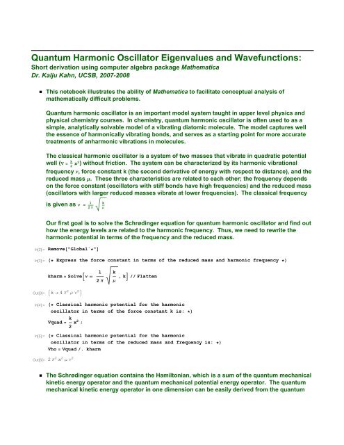
<strong>Quantum</strong> <strong>Harmonic</strong> <strong>Oscillator</strong> <strong>Eigenvalues</strong> <strong>and</strong> <strong>Wavefunctions</strong>:<br />
Short derivation using computer algebra package Mathematica<br />
Dr. Kalju Kahn, UCSB, 2007-2008<br />
ü<br />
This notebook illustrates the ability of Mathematica to facilitate conceptual analysis of<br />
mathematically difficult problems.<br />
<strong>Quantum</strong> harmonic oscillator is an important model system taught in upper level physics <strong>and</strong><br />
physical chemistry courses. In chemistry, quantum harmonic oscillator is often used to as a<br />
simple, analytically solvable model of a vibrating diatomic molecule. The model captures well<br />
the essence of harmonically vibrating bonds, <strong>and</strong> serves as a starting point for more accurate<br />
treatments of anharmonic vibrations in molecules.<br />
The classical harmonic oscillator is a system of two masses that vibrate in quadratic potential<br />
well (V k 2 x2 ) without friction. The system can be characterized by its harmonic vibrational<br />
frequency n, force constant k (the second derivative of energy with respect to distance), <strong>and</strong> the<br />
reduced mass m. These three characteristics are related to each other; the frequency depends<br />
on the force constant (oscillators with stiff bonds have high frequencies) <strong>and</strong> the reduced mass<br />
(oscillators with larger reduced masses vibrate at lower frequencies). The classical frequency<br />
is given as 1 k<br />
2 <br />
Our first goal is to solve the Schrødinger equation for quantum harmonic oscillator <strong>and</strong> find out<br />
how the energy levels are related to the harmonic frequency. Thus, we need to rewrite the<br />
harmonic potential in terms of the frequency <strong>and</strong> the reduced mass.<br />
In[2]:=<br />
In[3]:=<br />
Remove"Global`"<br />
Express the force constant in terms of the reduced mass <strong>and</strong> harmonic frequency <br />
kharm Solve 1<br />
2 k<br />
,kFlatten<br />
Out[3]=<br />
In[4]:=<br />
k 4 2 2 <br />
Classical harmonic potential for the harmonic<br />
oscillator in terms of the force constant k is: <br />
Vquad k 2 x2 ;<br />
In[5]:=<br />
Classical harmonic potential for the harmonic<br />
oscillator in terms of the reduced mass <strong>and</strong> frequency is: <br />
Vho Vquad . kharm<br />
Out[5]= 2 2 x 2 2<br />
ü<br />
The Schrødinger equation contains the Hamiltonian, which is a sum of the quantum mechanical<br />
kinetic energy operator <strong>and</strong> the quantum mechanical potential energy operator. The quantum<br />
mechanical kinetic energy operator in one dimension can be easily derived from the quantum
2 QUantHO_Waven.nb<br />
mechanical momentum operator (p = -i h<br />
2 p<br />
∂<br />
) by recalling the that the relationship between the<br />
∂ x<br />
kinetic energy <strong>and</strong> the momentum is: E kin = m v 2<br />
= p2<br />
. In the case of harmonic oscillator, the<br />
2 2 m<br />
action of a quantum mechanical potential operator is identical to the multiplication with the<br />
classical potential.<br />
In[6]:= Hamiltonian for the <strong>Quantum</strong> <strong>Harmonic</strong> <strong>Oscillator</strong>: H H kin H pot <br />
Hf <br />
h2<br />
Dtf, x, 2 Vho f<br />
8 2 Out[6]=<br />
2f 2 x 2 2 h2 Dtf, x, 2<br />
8 2 <br />
In[7]:= Solving the Vibrational Schrødinger Equation: H E <br />
VibrWF DSolve Hx Energyv x, x, x<br />
Out[7]=<br />
h 2 Energyv<br />
x C2 ParabolicCylinderD , 2 2 x <br />
2h<br />
h<br />
<br />
h 2 Energyv<br />
C1 ParabolicCylinderD , 2 2 x <br />
2h<br />
h<br />
<br />
In[8]:=<br />
Consider solutions with real variables only <br />
solnHerm FunctionExp<strong>and</strong>x . VibrWF . C2 0<br />
Out[8]=<br />
h 2 Energyv<br />
<br />
2<br />
4h<br />
2 2 x 2 <br />
h 2 Energyv<br />
h C1 HermiteH , 2 x <br />
2h<br />
h<br />
<br />
In[9]:=<br />
Obtain allowed energies by restricting Hermite polynomials to integer orders <br />
Env Solve 2 Energyv h <br />
0 v, Energyv<br />
2h<br />
EnHO TableEnergyv .Env, v, 0, 2 Flatten<br />
Out[9]=<br />
Energyv 1 h 1 2v <br />
2<br />
Out[10]=<br />
h <br />
2 , 3h<br />
2 , 5h<br />
2 <br />
ü<br />
We see that the concept of quantized vibrational energy states (v = 0, 1, 2, 3 ... ) arises naturally<br />
from the discrete spectrum of physically realistic eigenvalues of the solution to the vibrational<br />
Schrødinger equation. This spectrum can be experimentally probed using infrared<br />
spectroscopy.<br />
In[11]:=<br />
General vibrational wavefunction <br />
v, x SimplifysolnHerm . Env Flatten<br />
Out[11]=<br />
2 v2 2 2 x 2 <br />
h C1 HermiteHv, 2 x <br />
h
Cell[TextData[{Cell[TextData[{ValueBox["FileName"]}], "Header"], Cell[" ", "Header", CellFrame -> {{0, 0.5}, {0, 0}}, CellFrameMargins<br />
-> 4], " ", Cell[TextData[{CounterBox["Page"]}], "PageNumber"]}], CellMargins -> {{Inherited, 0}, {Inherited, Inherited<br />
In[12]:=<br />
<br />
Integration constant is determined by requiring that 2 x 1 <br />
c0v, x : SolveIntegrateLastv, x 2 , x, , , Assumptions <br />
0 1, C1<br />
h<br />
vx v, x : v, x . Lastc0v, x<br />
In[14]:=<br />
Some of the wave functions are <br />
v x FullSimplifyTablev, x . Lastc0v, x, v, 0, 2 Flatten;<br />
gv GridPartitionTablev, v, 0, 2, 1, Spacings 0, 2;<br />
gwf GridPartition v x, 1;<br />
gho GridPartitionEnHO, 1, Spacings 0, 2;<br />
GridPartitiongv, gwf, gho, 3, Frame All<br />
0<br />
2 2 2 x 2 <br />
h<br />
14 <br />
h 14<br />
h <br />
2<br />
Out[18]=<br />
1<br />
4 2 2 x 2 <br />
h 54 x <br />
h 14<br />
h<br />
3h<br />
2<br />
2<br />
2 2 x 2 <br />
h<br />
14 <br />
h 14 h8 2 x 2 <br />
h<br />
5h<br />
2<br />
In[19]:=<br />
Verify that the ground state wavefunction is indeed<br />
the same as expressed via in the traditional treatment <br />
0 x 0, x<br />
Out[19]= 2 x2 <br />
2 14 <br />
h 14<br />
<br />
. Lastc00, x . 2 2 x 2 <br />
<br />
h<br />
x2<br />
2<br />
. <br />
h <br />
4 2
4 QUantHO_Waven.nb<br />
ü<br />
In[20]:=<br />
Next we plot the vibrational energy levels <strong>and</strong> associated wavefunctions for carbon monoxide<br />
molecule. Because of its chemical stability <strong>and</strong> permanent dipole moment, the vibrational<br />
spectrum of CO is experimentally well characterized. For consistency with the traditional<br />
infrared nomenclature, the energy on the y-axis is expressed in wavenumber (cm -1 ) units. The<br />
internuclear distance on the x-axis is in meters with the equilibrium internuclear distance set to<br />
zero.<br />
PhysicalConstants`<br />
Planck Constant h in appropriate units is: <br />
h <br />
Kilogram 100 cm2<br />
PlanckConstant . Joule <br />
Second 2<br />
<br />
Second<br />
cm 2 Kilogram<br />
Reduced mass of carbon monoxide in kilograms is: <br />
12 16<br />
<br />
12 16 ProtonMass 1<br />
Kilogram ;<br />
Experimental harmonic frequency in wavenumber units is: <br />
waven 2168 cm 1 cm;<br />
<strong>Harmonic</strong> frequency in appropriate cm units is: <br />
waven SpeedOfLight . Meter 100 cm <br />
Second<br />
;<br />
cm<br />
Square of the speed of light in appropriate cm units is: <br />
cc SpeedOfLight 2 . Meter 100 cm Second2<br />
;<br />
cm 2<br />
Bond force constant in appropriate units is: <br />
fc k . kharm;<br />
;<br />
ü<br />
The first five energy levels <strong>and</strong> wave functions are shown below. Note that the magnitude of<br />
each of the wavefunctions is scaled arbitrarily to fit below the next energy level. The spacing<br />
between the energy levels is not scaled <strong>and</strong> corresponds to the experimental harmonic<br />
frequency ( 2168 cm 1 ).<br />
In[29]:= PlotEvaluate Append Table3 10 2 vx v, x v 1 2<br />
x, 1.5 10 9 , 1.5 10 9 , Filling Tablev v 1 2<br />
0.006 cc fc x2<br />
waven, v, 0, 4 , ,<br />
2<br />
waven, v, 1, 5, AxesLabel x ,"E"<br />
Out[29]=
Cell[TextData[{Cell[TextData[{ValueBox["FileName"]}], "Header"], Cell[" ", "Header", CellFrame -> {{0, 0.5}, {0, 0}}, CellFrameMargins<br />
-> 4], " ", Cell[TextData[{CounterBox["Page"]}], "PageNumber"]}], CellMargins -> {{Inherited, 0}, {Inherited, Inherited<br />
The first five energy levels <strong>and</strong> squares of associated wave functions are shown below. Note<br />
that the magnitude of each of the squared wavefunctions is scaled arbitrarily to fit below the<br />
next energy level. Recall that the square of the wavefunction gives the probability; the plot<br />
below thus shows probability distributions in different vibrational states. For example, the<br />
most probable bond distance in the ground state CO corresponds to the equilibrium distance at<br />
the bottom of the potential well.<br />
In[30]:=<br />
Plot<br />
Evaluate Append Table1.4 10 6 vx v, x vx v, x v 1 2<br />
waven, v, 0, 4 ,<br />
0.006 cc fc x2<br />
,<br />
2<br />
x, 1.5 10 9 , 1.5 10 9 , Filling Tablev v 1 2<br />
waven, v, 1, 5,<br />
AxesLabel x, "E", PlotRange All<br />
Out[30]=